High-probability Convergence Bounds for Non-convex Stochastic Gradient Descent

Abstract

Stochastic gradient descent is one of the most common iterative algorithms used in machine learning. While being computationally cheap to implement, recent literature suggests it may have implicit regularization properties that prevent over-fitting. This paper analyzes the properties of stochastic gradient descent from a theoretical standpoint to help bridge the gap between theoretical and empirical results. Most theoretical results either assume convexity or only provide convergence results in mean, while this paper proves convergence bounds in high probability without assuming convexity. Assuming strong smoothness, we prove high probability convergence bounds in two settings: (1) assuming the Polyak-Łojasiewicz inequality and norm sub-Gaussian gradient noise and (2) assuming norm sub-Weibull gradient noise. In the first setting, we combine our convergence bounds with existing generalization bounds in order to bound the true risk and show that for a certain number of epochs, convergence and generalization balance in such a way that the true risk goes to the empirical minimum as the number of samples goes to infinity. In the second setting, as an intermediate step to proving convergence, we prove a probability result of independent interest. The probability result extends Freedman-type concentration beyond the sub-exponential threshold to heavier-tailed martingale difference sequences.

1 Introduction

Stochastic gradient descent (SGD) is an algorithm for minimizing a cost function by relying on noisy estimates of the gradient. Theoretical results provide guarantees for the convergence of SGD to a stationary point via convergence bounds in mean, almost sure convergence, or convergence bounds in probability. All three depend on the properties of both the cost function and the noise distribution. In particular, we consider the follow settings:

• where the cost function is strongly smooth and satisfies the Polyak-Łojasiewicz (PL) inequality, and the noise is norm sub-Gaussian;

• where the cost function is strongly smooth, and the noise is norm sub-Gaussian; and

• where the cost function is strongly smooth and Lipschitz continuous, and the noise is norm sub-Weibull.

The PL inequality is a weaker form of strong convexity that does not imply convexity and is motivated by recent papers that prove PL-type inequalities for neural nets (Li and Yuan, 2017; Allen-Zhu et al, 2019b, a; Liu et al, 2020). The sub-Weibull noise assumption is weaker than the sub-Gaussian noise assumption and is motivated by recent results where the noise for empirical risk minimization applied to particular problems is not sub-Gaussian for small batch-sizes (Gürbüzbalaban et al, 2021; Şimşekli et al, 2019; Panigrahi et al, 2019).

Almost sure convergence to a first-order stationary point can be proved assuming only strong smoothness and a weak assumption on the noise (Bertsekas and Tsitsiklis, 2000; Patel, 2021). In this case, the mean convergence rate of the squared gradient norm to zero is $O(1/\sqrt{T})$, where $T$ denotes the number of iterations (Ghadimi and Lan, 2013; Khaled and Richtárik, 2020). It is also possible to prove a matching almost sure convergence rate (Sebbouh et al, 2021). If the PL inequality is also assumed, then the mean convergence rate of the cost function of the iterates to the minimum is $O(1/T)$ (Karimi et al, 2016; Khaled and Richtárik, 2020). However, a convergence guarantee is generally required with some arbitrary probability, $1-\delta$. A mean convergence rate is acceptable when it is possible to re-run SGD many times, since Markov’s inequality can be applied and the best run chosen. On the other hand, if only one run of SGD is allowed, then the $(1/\delta)$-dependence of Markov’s inequality quickly blows up. What is needed is a bound with logarithmic dependence on $1/\delta$. Assuming strong smoothness and norm sub-Gaussian noise, Li and Orabona (2020) prove a $O(\log(T)\log(T/\delta)/\sqrt{T})$ convergence bound. We do not know of any other convergence bounds in the strongly smooth setting that have only logarithmic dependence on $\delta$. In Section 2, we introduce the preliminaries; delineate the optimization assumptions, the types of convergence, and the noise assumptions; and discuss how our results fit into the broader literature.

Section 3 is dedicated to setting (S1). In Section 3.1, we prove a $O(\log(1/\delta)/T)$ convergence bound, which matches the optimal convergence rate in mean of $O(1/T)$. In Section 3.2, we focus on the statistical learning framework and consider SGD with a mini-batch and sub-Gaussian (as a random vector) noise. We prove, as a simple application of our convergence analysis, a bound on the true risk that goes to the empirical minimum as the sample size increases to infinity. The bound has $1/\sqrt{\delta}$ dependence on $\delta$, which, while not logarithmic, is better than the $1/\delta$ that comes from the mean convergence bound and Markov’s inequality. Furthermore, it is based on a conservative step-size constant and a fixed number of epochs, corresponding to practice where a better step-size constant for convergence may paradoxically fit random labels (Zhang et al, 2017) and where early stopping is used to avoid over-fitting.

Section 4 is dedicated to setting (S2). The convergence results are presented in Section 4.2. For setting (S2a), we prove a $O(\log(T)\log(1/\delta)/\sqrt{T})$ convergence bound, improving the log factors of the bound in Li and Orabona (2020). Moreover, our bound is for an argmin over a small number of iterates, while the bound in Li and Orabona (2020) is for an argmin over all of the iterates. This last point is an independent contribution of the paper and is presented in Theorem 13 where we call it “efficient post-processing.” For setting (S2b), we prove a $O(\log(T/\delta)^{\theta}\log(1/\delta)/\sqrt{T})$ convergence bound, where $\theta$ is the sub-Weibull tail weight. On our way to proving the non-convex (without the PL inequality) convergence bounds, we prove a Freedman-type inequality for martingale difference sequences with sub-Weibull tails. Previously, such inequalities only allowed for, at most, sub-exponential tails, as in Fan et al (2015). In order to push beyond the sub-exponential boundary, we used the moment generating function truncation techniques of Bakhshizadeh et al (2020). The additional constants that the sub-Weibull noise introduces fortunately balance in such a way that we are still able to get a $1/\sqrt{T}$ sub-linear convergence rate up to logarithmic factors. Section 4.1 presents the sub-Weibull Freedman-type concentration inequality.

Section 5 provides numerical examples to elucidate the theoretical results. In particular, SGD is applied to various neural-net-based synthetic problems.

2 Preliminaries

We are interested in the unconstrained optimization problem

$$\min_{x\in\mathbb{R}^{d}}f(x),$$ (1)

where $f:\mathbb{R}^{d}\rightarrow\mathbb{R}$ is a differentiable function, and the SGD iteration

$$x_{t+1}=x_{t}-\eta_{t}g_{t}\leavevmode\nobreak\ \forall t\in\mathbb{N}\cup\{0\},$$

where $g_{t}\in\mathbb{R}^{d}$ is an estimate of $\nabla f(x_{t})$, $\eta_{t}$ is the step-size, and $x_{0}\in\mathbb{R}^{d}$ is the initial point. Formalized in this way, it remains to specify: (1) the properties of $f$, the cost function; (2) the types of convergence of $(x_{t})$ to a stationary point; and (3) the properties of the noise $e_{t}\coloneqq\nabla f(x_{t})-g_{t}$. We restrict our attention to the setting where $x_{0}$ is deterministic, but the results easily extend to the setting where $x_{0}$ is a random vector.

One of the main examples of Eq. (1) is the stochastic approximation problem: $f=\mathbb{E}\left[F(\cdot,\xi)\right]$ where $(\Omega,\mathcal{F},P)$ is a probability space and $F:\mathbb{R}^{d}\times\Omega\rightarrow\mathbb{R}$ (Nemirovski et al, 2009; Ghadimi and Lan, 2013; Bottou and Bousquet, 2008). In this case, we independently sample $\xi_{0},\xi_{1},\ldots$ and set $g_{t}=\nabla F(x_{t},\xi_{t})$.

Note that we frequently use big-$O$ and little-$o$ notation. When comparing two sequences of real numbers, $(a_{t})$ and $(b_{t})$: $a_{t}=o(b_{t})$ if $\lim a_{t}/b_{t}=0$, $a_{t}=O(b_{t})$ if $\limsup|a_{t}|/b_{t}<\infty$, $a_{t}=\Omega(b_{t})$ if $b_{t}=O(a_{t})$, $a_{t}=\omega(b_{t})$ if $b_{t}=o(a_{t})$, and $a_{t}=\Theta(b_{t})$ if $a_{t}=O(b_{t})$ and $a_{t}=\Omega(b_{t})$. We use $a_{t}=\text{poly}(b_{t})$ to denote that there is a polynomial function $p$ such that $a_{t}=O(p(b_{t}))$. Finally, we use $[n]$ to denote the set $\{1,\ldots,n\}$.

2.1 Optimization Assumptions

Throughout the paper we implicitly assume $\text{argmin}_{x\in\mathbb{R}^{d}}f(x)$ is non-empty so it is a well-posed problem, and hence $f^{\star}\coloneqq\min_{x\in\mathbb{R}^{d}}f(x)>-\infty$. We assume that $f$ is $L$-strongly smooth (or $L$-smooth for short) for a given $L>0$; i.e., $f\in C^{1}$ and its gradient is $L$-Lipschitz continuous.

A function $f$ is $\mu$-Polyak-Łojasiewicz (or $\mu$-PL for short) if $\|\nabla f(x)\|^{2}\geq 2\mu(f(x)-f^{\star})\leavevmode\nobreak\ \forall x\in\mathbb{R}^{d}$. Some examples of problems with PL objectives are logistic regression (Karimi et al, 2016) and matrix factorization (Sun and Luo, 2016). Deep linear neural networks satisfy the PL inequality in large regions of the parameter space (Charles and Papailiopoulos, 2018, Thm. 4.5), as do two-layer neural networks with an extra identity mapping (Li and Yuan, 2017). Furthermore, sufficiently wide recurrent neural networks satisfy the PL inequality locally around random initialization (Allen-Zhu et al, 2019b, a; Liu et al, 2020). While strong convexity implies the PL inequality, a PL function need not even be convex, hence the PL condition is considerably more applicable than strong convexity in the context of neural networks.

Recall that we focus on two main settings with regards to optimization assumptions: (S1) the case where $f$ is $L$-smooth and satisfies the PL inequality, and convergence is to a global optima, and (S2) the more general case where $f$ is $L$-smooth, and convergence is to a stationary point. We do not require convexity in either case, though we sometimes refer to the second case as the “non-convex” case since the convergence is to a stationary point as is typical for non-convex analysis.

We also note that some of the non-convex results require $f$ to be $\rho$-Lipschitz continuous; the paper will state when this assumption is needed. Lipschitz continuity of $f$ follows immediately if the iterates are bounded. This might lead one to consider projected SGD, but there are certain issues preventing us from doing so which we discuss in Appendices E and J.

Further details on standard optimization terminology and results are in Appendix A.

2.2 Types of Convergence

To analyze the convergence of SGD, we define a sequence of pertinent random variables $(X_{T})$. In the PL setting, since the PL inequality implies that all stationary points are global minima, we set $X_{T}=f(x_{T})-f^{\star}$. In the non-convex setting, since SGD may converge to a stationary point, we set $X_{T}=\min_{0\leq t\leq T-1}\|\nabla f(x_{t})\|^{2}$ or $X_{T}=\|\nabla f(y_{T})\|^{2}$ where $y_{T}$ is carefully chosen from $x_{0}\ldots,x_{T-1}$. Note that we do not consider iterate averaging in either case because the usual trick using Jensen’s inequality requires convexity, so a bound on the averaged error (i.e., the regret) does not translate to a bound on the error of the average iterate.

Results bounding $\mathbb{E}\left[X_{T}\right]$ (expected/mean/$L_{1}$ convergence) for SGD are common but strong results bounding $X_{T}$ with $(1-\delta)$-confidence are relatively rare. See Nemirovski et al (2009), Kakade and Tewari (2008), Rakhlin et al (2012), Hazan and Kale (2014), Harvey et al (2019b), and Harvey et al (2019a) for such bounds in the non-smooth convex setting. Clearly, guarantees with high confidence are quite desirable. We can go from expectation to probability via Markov’s inequality, $P\left(X_{T}\leq\mathbb{E}\left[X_{T}\right]/\delta\right)\geq 1-\delta$, but we want the dependence on $\delta$ to be better than $1/\delta$ multiplicative dependence. In particular, we want $\text{poly}(\log(1/\delta))$, which we call “high probability” dependence, as opposed to $\text{poly}(1/\delta)$, which we call “low probability” dependence.

One way to get high probability dependence from Markov’s inequality is through probability amplification, which involves taking multiple runs and picking the best run based on a validation set; for example, Exer. 13.1 of Shalev-Shwartz and Ben-David (2014) describes probability amplification for the true risk. Their procedure takes $\Theta(\log(1/\delta))$ runs and $\Theta(\log(1/\delta)/\epsilon^{2})$ validation samples and relies on the boundedness of the loss function. Davis et al (2021) describe probability amplification for convergence in the strongly convex setting. They use strong convexity to apply robust distance estimation and get around the $\Omega(1/\epsilon^{2})$ sample requirement for mean estimation (Catoni, 2012). Thm. 2.4 of Ghadimi and Lan (2013) describes probability amplification for convergence in the non-convex setting. Their procedure takes $\Theta(\log(1/\delta))$ runs and $\Theta(\log(1/\delta)/(\delta\epsilon))$ validation samples and relies on the boundedness of the variance of the norm of the gradient noise.

The above probability amplification techniques involve both an optimization cost and a validation cost. Re-running SGD multiple times clearly increases the optimization cost, so our goal is to prove high probability convergence bounds for a single run of SGD that match the mean convergence bounds without increasing the validation cost. The only bound we have that requires validation is the non-convex bound since it is in terms of $\min_{0\leq t\leq T-1}\|\nabla f(x_{t})\|^{2}$. If we want a bound in terms of $\|\nabla f(x_{s})\|^{2}$ for a particular $s$, then we have to compute the argmin, which means performing validation on $T$ choices instead of $\Theta(\log(1/\delta))$. Fortunately, Theorem 13 shows that there is a workaround involving only $\Theta(\log(1/\delta))$ iterates, same as for multiple runs. Then the same validation step as in Ghadimi and Lan (2013) can be applied.

Further details on the convergence of random variables can be found in Appendix B.

2.3 Noise Assumptions

We make assumptions involving the bias, variance, and tail behavior of the noise $e_{t}$. First, let $(\Omega,\mathcal{F},P)$ be the underlying probability space and define the natural filtration $\mathcal{F}_{t}=\sigma(e_{0},\ldots,e_{t})\leavevmode\nobreak\ \forall t\geq 0$, $\mathcal{F}_{-1}=\{\emptyset,\Omega\}$. We assume the noise is unbiased, $\mathbb{E}\left[e_{t}\mid\mathcal{F}_{t-1}\right]=0$, and that the variance is bounded by a constant, $\mathbb{E}\left[\|e_{t}\|^{2}\mid\mathcal{F}_{t-1}\right]\leq\sigma^{2}$. It is possible to prove almost sure convergence of SGD in the smooth non-convex setting with weaker assumptions on the bias, namely that there is an additional noise term $\epsilon_{t}$ in the gradient with the properties $c_{1}\|\nabla f(x_{t})\|^{2}\leq-\langle\nabla f(x_{t}),\epsilon_{t}\rangle$ and $\|\epsilon_{t}\|\leq c_{2}\left(1+\|\nabla f(x_{t})\|\right)$ for all $t$, and on the variance, namely that $\mathbb{E}\left[\|e_{t}\|^{2}\mid\mathcal{F}_{t-1}\right]\leq\sigma^{2}\left(1+\|\nabla f(x_{t})\|^{2}\right)$ for all $t$ (Bertsekas and Tsitsiklis, 2000; Patel, 2021); but it is not clear how to do so for high probability convergence.

Next, while mean convergence rates do not require assumptions on the tail behavior of the noise, high probability convergence rates do. In particular, Nemirovski et al (2009) make the assumption $\mathbb{E}\left[\exp\left(\|e_{t}\|^{2}/\sigma^{2}\right)\right]\leq\exp(1)$, which corresponds to sub-Gaussian tail behavior. Note that this tail assumption implies the variance assumption via Jensen’s inequality. We consider sub-Gaussian, sub-exponential, and sub-Weibull noise (Vladimirova et al, 2020; Wong et al, 2020; Bakhshizadeh et al, 2020), defined below:

Definition 1.

A random variable $X$ is $K$-sub-Gaussian if $\mathbb{E}\left[\exp\left(X^{2}/K^{2}\right)\right]\leq 2$. See Prop. 2.5.2 of Vershynin (2018) for equivalent definitions.

Definition 2.

A random variable $X$ is $K$-sub-exponential if $\mathbb{E}\left[\exp\left(|X|/K\right)\right]\leq 2$. See Prop. 2.7.1 of Vershynin (2018) for equivalent definitions.

Definition 3.

A random variable $X$ is $K$-sub-Weibull($\theta$) if $\mathbb{E}\left[\exp\left((|X|/K)^{1/\theta}\right)\right]\leq 2$. The tail parameter $\theta$ measures the heaviness of the tail—higher values correspond to heavier tails—and the scale parameter $K$ gives us the following bound on the second moment, $\mathbb{E}\left[X^{2}\right]\leq 2\Gamma(2\theta+1)K^{2}$ (Lemma 22). See Thm 2.1 of Vladimirova et al (2020) for equivalent definitions. Note that sub-Gaussian and sub-exponential are special cases with $\theta=\frac{1}{2}$ and $\theta=1$, respectively.

While many works in the context of SGD consider errors modeled by sub-Gaussian distributions, we provide a brief discussion on the relevance of the sub-Weibull assumption. First, Vladimirova et al (2019) show that a Gaussian prior on the weights in a Bayesian neural network induces a sub-Weibull distribution on the weights with the optimal tail parameter for a particular layer proportional to its depth. Secondly, a series of recent papers (Gürbüzbalaban et al, 2021; Şimşekli et al, 2019; Panigrahi et al, 2019) suggest that SGD exhibits noise with tails that are heavier than sub-Gaussian. Nguyen et al (2019) and Hodgkinson and Mahoney (2021) suggest that the heavier-tailed noise of SGD may be vital to its ability to find machine learning models that perform well on unseen data.

To the best of the authors’ knowledge, all existing results for the high probability convergence rate of SGD assume norm sub-Gaussian noise. While the central limit theorem can be used to justify the sub-Gaussian noise assumption for mini-batch SGD with large batch-sizes, it cannot for small batch-sizes. One alternative distribution that has been suggested is the $\alpha$-stable distribution with $\alpha<2$, which has infinite variance. Şimşekli et al (2019) and Gürbüzbalaban et al (2021) empirically determine the tail-index for stochastic gradient noise assuming it follows an $\alpha$-stable distribution and Zhang et al (2019) prove mean convergence bounds for clipped SGD in this setting. However, none of these papers actually show that the noise is $\alpha$-stable, or even that it has infinite variance. On the other hand, Panigrahi et al (2019) test when the noise is or is not Gaussian. They find that the noise is Gaussian for a batch-size of 4096, is not for a batch-size of 32, and starts out Gaussian then becomes non-Gaussian for a batch-size of 256.

Even though sub-Weibull noise has finite variance, by relaxing the noise assumption from sub-Gaussian to sub-Weibull, we are taking a step towards a more realistic analysis of SGD.

Remark 4.

Our noise assumptions will be on the Euclidean norm of the noise vector. We note that it is straightforward to show that if $(e_{i})\in\mathbb{R}^{d}$ is component-wise sub-Weibull, then its norm is sub-Weibull. Concretely, assume $e_{i}$ is $K_{i}$-sub-Weibull($\theta$) for $i=1,\ldots,d$. Let ${\left|\kern-1.07639pt\left|\kern-1.07639pt\left|\cdot\right|\kern-1.07639pt\right|\kern-1.07639pt\right|}_{\theta}$ denote the Orlicz norm (infimum of all possible scale parameters given the tail parameter $\theta$). Then

$${\left|\kern-1.07639pt\left|\kern-1.07639pt\left|\leavevmode\nobreak\ \vphantom{\big{|}}\|(e_{i})\|\leavevmode\nobreak\ \right|\kern-1.07639pt\right|\kern-1.07639pt\right|}_{\theta}={\left|\kern-1.07639pt\left|\kern-1.07639pt\left|\left(\sum_{i=1}^{d}e_{i}^{2}\right)^{1/2}\right|\kern-1.07639pt\right|\kern-1.07639pt\right|}_{\theta}={\left|\kern-1.07639pt\left|\kern-1.07639pt\left|\sum_{i=1}^{d}e_{i}^{2}\right|\kern-1.07639pt\right|\kern-1.07639pt\right|}_{2\theta}^{1/2}\leq\left(\sum_{i=1}^{d}{\left|\kern-1.07639pt\left|\kern-1.07639pt\left|e_{i}^{2}\right|\kern-1.07639pt\right|\kern-1.07639pt\right|}_{2\theta}\right)^{1/2}=\left(\sum_{i=1}^{d}{\left|\kern-1.07639pt\left|\kern-1.07639pt\left|e_{i}\right|\kern-1.07639pt\right|\kern-1.07639pt\right|}_{\theta}^{2}\right)^{1/2}=\|(K_{i})\|.$$

Note that the components may be dependent.

2.4 Prior Work and Contributions

Assuming strong smoothness and strong convexity, the tight mean convergence rate is $O(1/T)$ (Nemirovski et al, 2009). The same mean convergence rate can be shown assuming strong smoothness and the PL inequality (Karimi et al, 2016; Orvieto and Lucchi, 2019). Assuming strong smoothness, the PL inequality, and norm sub-Gaussian noise, our Theorem 6 provides a matching $O(\log(1/\delta)/T)$ convergence rate for the high probability case. Our theorem depends on Proposition 5 which is a novel probability result, essentially saying that adding two kinds of noise to a contracting sequence—sub-Gaussian noise with variance depending on the sequence itself and sub-exponential noise—results in a sub-exponential sequence.

We then apply our convergence analysis to the statistical learning problem. We find that by taking a more conservative step-size, the training error goes to zero slower, but the generalization error also increases slower in such a way that we can balance the two. In particular, we find a bound that supports running multiple, but limited epochs of mini-batch SGD. For papers developing the generalization analysis that we use, see Bousquet and Elisseeff (2002), Elisseeff et al (2005), and Hardt et al (2016). Other relevant papers are Mou et al (2018), Charles and Papailiopoulos (2018), Shalev-Shwartz et al (2010), Feldman and Vondrak (2019), and Bousquet et al (2020). Note that Feldman and Vondrak (2019) prove high probability generalization bounds for SGD, but only in the convex setting. Also, they balance their generalization result with the convergence result of Harvey et al (2019b).

Assuming strong smoothness and convexity, the tight mean convergence rate of the squared gradient norm is $O(1/\sqrt{T})$ (Nemirovsky and Yudin, 1983, Thm. 5.3.1). In fact, this is the optimal rate for all stochastic first-order methods assuming only strong smoothness (and not convexity) (Arjevani et al, 2019). The same mean convergence rate can be shown for SGD assuming only strong smoothness (Ghadimi and Lan, 2013). However, the result of Ghadimi and Lan (2013) requires a constant step-size equal to $\Theta(1/\sqrt{T})$ to get the $O(1/\sqrt{T})$ convergence rate. On the other hand, for a $\Theta(1/\sqrt{t})$ step-size sequence, the rate is $O(\log(T)/\sqrt{T})$. Assuming strong smoothness and norm sub-Gaussian noise, Li and Orabona (2020) prove a $O(\log(T)\log(T/\delta)/\sqrt{T})$ convergence rate. Our non-convex convergence result, Theorem 12, improves this to $O(\log(T)\log(1/\delta)/\sqrt{T})$ and, assuming strong smoothness, Lipschitz continuity, and norm sub-Weibull noise, proves a $O((\log(T/\delta)^{\theta}\log(1/\delta)+\log(T)\log(1/\delta)^{2\theta})/\sqrt{T})$ convergence rate. To the best of the authors’ knowledge, all existing results for the high probability convergence rate of SGD assume norm sub-Gaussian noise.

Another contribution is that our non-convex convergence rates are for an argmin over $\lceil\log(1/\delta)\rceil$ iterates while the bound of Li and Orabona (2020) is for an argmin over all of the iterates. We are able to restrict the number of iterates we have to minimize over via a post-processing sampling strategy that extends the sampling strategy of Ghadimi and Lan (2013) from mean to probability. The crux of the proof is Lemma 33. Then the minimization step can be done via a validation set as in Ghadimi and Lan (2013). One takeaway from our convergence rate is that the optimal step-size constant for mean convergence only depends on the variance, whereas the optimal step-size constant for high probability convergence depends on $\delta$ and $\theta$ as well.

Our proof of Theorem 12 depends on a novel probability result, Proposition 11. The probability result is of independent interest because it extends, for the first time, Freedman-type concentration inequalities beyond the sub-exponential threshold (Freedman, 1975; Fan et al, 2015; Harvey et al, 2019b). In particular, we use the truncated MGF technique of Bakhshizadeh et al (2020) to generalize the Generalized Freedman inequality of Harvey et al (2019b) from sub-Gaussian to sub-Weibull martingale difference sequences.

3 Smooth, PL, Sub-Gaussian Setting

In this section, we assume the PL inequality and norm sub-Gaussian gradient noise. In Section 3.1, we consider a stochastic recursion with two types of noise: sub-Gaussian with dependence on the main sequence and sub-exponential. In Proposition 5, we prove that the main sequence is sub-exponential. Then, we show that the error of SGD satisfies just such a recursion, allowing us to prove the high probability convergence bound in Theorem 6.

In Section 3.2, we consider the statistical learning framework as an example. It turns out a more conservative step-size constant is needed, which gives a slower convergence rate; this is shown in Theorem 9. Finally, we provide the resulting true risk bound in Theorem 10.

3.1 Convergence

We start our analysis by recalling that strong smoothness of the function $f$ implies that

$$f(x) \leq f(y)+\langle\nabla f(y),x-y\rangle+\frac{L}{2}\|x-y\|^{2}$$

for any $x,y\in\mathbb{R}^{d}$. Set $x=x_{t+1}$ and $y=x_{t}$; then, by subtracting $f^{\star}$ from both sides and substituting in $x_{t+1}=x_{t}-\eta_{t}g_{t}=x_{t}-\eta_{t}(\nabla f(x_{t})-e_{t})$, we get

$$f(x_{t+1})-f^{\star} \leq f(x_{t})-f^{\star}-\eta_{t}\left(1-\frac{L\eta_{t}}{2}\right)\|\nabla f(x_{t})\|^{2}+\eta_{t}(1-L\eta_{t})\langle\nabla f(x_{t}),e_{t}\rangle+\frac{L\eta_{t}^{2}}{2}\|e_{t}\|^{2}$$ (2)

$$\leq f(x_{t})-f^{\star}-\frac{\eta_{t}}{2}\|\nabla f(x_{t})\|^{2}+\eta_{t}(1-L\eta_{t})\langle\nabla f(x_{t}),e_{t}\rangle+\frac{L\eta_{t}^{2}}{2}\|e_{t}\|^{2}$$

$$\leq(1-\mu\eta_{t})(f(x_{t})-f^{\star})+\eta_{t}(1-L\eta_{t})\langle\nabla f(x_{t}),e_{t}\rangle+\frac{L\eta_{t}^{2}}{2}\|e_{t}\|^{2}$$ (3)

where the 2nd line follows if $\eta_{t}\leq 1/L$, and the 3rd line follows if $f$ satisfies the PL inequality.

In Theorem 6, we will show that the sub-Gaussian assumption on $e_{t}$ causes the second term to be sub-Gaussian with an implicit dependence on $f(x_{t})-f^{\star}$ and the third term to be sub-exponential. In the following proposition, we show that such noise ends up causing $f(x_{t})-f^{\star}$ to be sub-exponential, identifying $X_{t}\approx t^{2}(f(x_{t})-f^{\star})$. Below, the indices for all sequences are the natural numbers unless otherwise specified.

Proposition 5.

Let $(\Omega,\mathcal{F},(\mathcal{F}_{i}),P)$ be a filtered probability space. Let $(X_{i})$, $(\hat{w}_{i})$, and $(\hat{v}_{i})$ be adapted to $(\mathcal{F}_{i})$, and $X_{0}$ deterministic. Let $(\alpha_{i})$, $(\beta_{i})$, and $(\gamma_{i})$ be non-negative sequences. Assume $X_{i}$ and $\hat{v}_{i}$ are non-negative almost surely. Assume $\mathbb{E}[\exp(\lambda\hat{w}_{i})\mid\mathcal{F}_{i-1}]\leq\exp(\frac{\lambda^{2}}{2}\beta_{i}^{2}X_{i})$ for all $\lambda\in\mathbb{R}$ and $\mathbb{E}[\exp(\lambda\hat{v}_{i})\mid\mathcal{F}_{i-1}]\leq\exp(\lambda\gamma_{i})$ for all $\lambda\in[0,\gamma_{i}^{-1}]$. Assume

$$X_{i+1}\leq\alpha_{i}X_{i}+\hat{w}_{i}+\hat{v}_{i}.$$

Then, for any $(K_{i})$ such that $K_{0}\geq X_{0}$ and, for all $i\geq 0$, $K_{i+1}^{2}\geq(\alpha_{i}K_{i}+2\gamma_{i})K_{i+1}+\beta_{i}^{2}K_{i}$, and any $n\geq 0$, we have, $\text{w.p.}\geq 1-\delta$ for all $\delta\in(0,1)$,

$$X_{n}\leq K_{n}\log(e/\delta).$$

The proof is in Appendix C. It is similar to the proof of Theorem 4.1 in Harvey et al (2019b) but with some key differences. There, the recursion is $X_{i+1}\leq\alpha_{i}X_{i}+\hat{w}_{i}\sqrt{X_{i}}+v_{i}$ where $\mathbb{E}\left[\exp(\lambda\hat{w}_{i})\mid\mathcal{F}_{i-1}\right]\leq\exp\left(\frac{\lambda^{2}}{2}\beta_{i}^{2}\right)$ and $v_{i}$ is deterministic. We had to move the implicit dependence of the sub-Gaussian term inside of the moment generating function in order to apply it to the inner product term in Eq. (3). We also had to allow $v_{i}$ to be a sub-exponential random variable $\hat{v}_{i}$, and so applied Cauchy-Schwarz, which contributed the 2 in the recursion for $(K_{i})$.

With Proposition 5, we are ready to prove high probability convergence for SGD with a particular $\Theta(1/t)$ step-size sequence.

Theorem 6.

Assume $f$ is $L$-smooth and $\mu$-PL and that, conditioned on the previous iterates, $e_{t}$ is centered and $\|e_{t}\|$ is $\sigma$-sub-Gaussian. Then, SGD with step-size

$$\eta_{t}=\frac{2t+4\kappa-1}{\mu(t+2\kappa)^{2}},$$

where $\kappa=L/\mu$, constructs a sequence $(x_{t})$ such that, $\text{w.p.}\geq 1-\delta$ for all $\delta\in(0,1)$,

$$f(x_{T})-f^{\star} =O\left(\frac{L\sigma^{2}\log(1/\delta)}{\mu^{2}T}\right).$$

The proof is in Appendix D. The convergence bound of Theorem 6 matches the optimal convergence rate in mean of $O(1/T)$ and has $\log(1/\delta)$ dependence on $\delta$.

Remark 7.

It is natural to ask whether we can relax the sub-Gaussian assumption to a sub-Weibull assumption. In Proposition 5, we need a bound on the moment generating functions of both $\hat{w}_{i}$ and $\hat{v}_{i}$. But, if $\|e_{t}\|$ is $\sigma$-sub-Weibull($\theta$) with $\theta>1/2$, then $\|e_{t}\|^{2}$ is $\sigma^{2}$-sub-Weibull($2\theta$). Thus, $\hat{v}_{i}$ would be sub-Weibull with tail parameter greater than 1, and so may have an infinite moment generating function for all $\lambda>0$.

3.2 Generalization

A particular example of Eq. (1) that we are concerned with is the supervised statistical learning problem (Shalev-Shwartz and Ben-David, 2014; Mohri et al, 2018). Consider a data set $S\coloneqq(s_{i})_{i=1}^{n}\sim\mathcal{D}^{n}$ consisting of $n$ iid samples, $s_{i}\sim\mathcal{D}$ for $i\in[n]$, where $\mathcal{D}$ is an arbitrary and unknown distribution. Let $\ell(x,s)$ measure the loss of the model parameterized by $x\in\mathbb{R}^{d}$ applied to the sample point $s$. Given $S$, let $F(x,i)=\ell(x,s_{i})$ and define the empirical risk

$$f(x)=\frac{1}{n}\sum_{i=1}^{n}\ell(x,s_{i})=\mathbb{E}_{i\sim U([n])}[F(x,i)].$$ (4)

Sometimes we write $f_{n}$ (and $f_{n}^{\star}=\min_{x}f_{n}(x)$) when we want to emphasize the dependence of $f$ on the samples, otherwise the $n$ is implicit. We will apply SGD to minimizing the empirical risk using the mini-batch gradient estimator

$$g(x,b)=\frac{1}{b}\sum_{i\in I}\nabla\ell(x,s_{i})$$

where $I$ is a uniform sample of $b$ indices sampled with replacement from $[n]$. In particular, we sample $g_{t}\sim g(x_{t},b_{t})$. However, the goal is actually to find an $x$ that has a small true risk

$$\tilde{f}(x)=\mathbb{E}_{s\sim\mathcal{D}}\leavevmode\nobreak\ \ell(x,s).$$

and we define $f^{\star}_{\infty}=\min_{x}\tilde{f}(x)$.

Applying SGD with many fewer than $n/b$ iterations can be thought of as a stochastic approximation to minimize $\tilde{f}$ directly, but most realistic scenarios take more than one-pass of the data in order to further reduce the training error, so we adopt the statistical learning framework for analysis. In this framework, we really care about $\tilde{f}(x_{T})-f^{\star}_{\infty}$, which we write as

$$\tilde{f}(x_{T})-f^{\star}_{\infty}=\underbrace{\tilde{f}(x_{T})-f_{n}(x_{T})}_{\text{generalization error}}+\underbrace{f_{n}(x_{T})-f_{n}^{\star}}_{\text{convergence error}}+\underbrace{f_{n}^{\star}-f^{\star}_{\infty}}_{\text{finite sample error}}.$$

Since the finite sample error depends only on the data and distribution $\mathcal{D}$ and not on the algorithm, we do not analyze it here; it is often assumed to be small, or at least dominated by the other terms. We will analyze the generalization error and convergence error separately. Unlike classical theory which bounds the generalization error by restricting $x$ to a low-complexity set, or by adding a regularization term, we use the implicit regularization of early stopping (Thm. 8), so generalization error is $\text{poly}(T)$. Meanwhile, convergence error decreases with iterates, and is $\text{poly}(1/T)$ (Thm. 9); Theorem 10 shows that for $T=\Theta(n/b)$, both the $\text{poly}(T)$ and $\text{poly}(1/T)$ terms decay to $0$ as the number of samples $n\to\infty$. Proofs for this section can be found in Appendix F.

The foundations for the interplay between stability and generalization go back to Devroye and Wagner (1979). Most recent results build off of Bousquet and Elisseeff (2002). In particular, the results of Elisseeff et al (2005) can be applied to the mean stability bound of Hardt et al (2016) to get a low probability generalization bound.

Theorem 8.

(Elisseeff et al, 2005; Hardt et al, 2016) Assume $\ell(x,s)\in[0,M]$ for all $x$ and $s$. Assume $\ell(\cdot,s)$ is $\rho$-Lipschitz and $L$-smooth for all $s$. Then, $T$ iterations of SGD with $\eta_{t}\leq c/(t+1)$ and $b_{t}=b$ satisfies, $\text{w.p.}\geq 1-\delta$ over $S$ and $(I_{t})$ for all $\delta\in(0,1)$,

$$\tilde{f}(x_{T})-f(x_{T}) \leq O\left(\sqrt{\frac{M\rho^{2}T^{Lc}(c+1/L)b}{n\delta}}\right).$$

Unfortunately the generalization bound in Thm. 8 depends on $1/\sqrt{\delta}$, which makes it a low probability bound. Furthermore, it grows with the number of iterations, counteracting the decay of the convergence error. Before proceeding, we need to prove a convergence rate for a more conservative step-size constant.

Theorem 9.

Assume $f$ is $L$-smooth and $\mu$-PL and that $\nabla f(x)-g(x,1)$ is centered and $\sigma/\sqrt{d}$-sub-Gaussian for all $x$. Then, $T$ iterations of SGD with $\eta_{t}=c/(t+1)$, where $c<1/\mu$ and $c\leq 1/L$, and $b_{t}=b$ satisfies, $\text{w.p.}\geq 1-\delta$ over $(I_{t})$ for all $\delta\in(0,1)$,

$$f(x_{T})-f^{\star} \leq O\left(\left(f(x_{0})-f^{\star}+\frac{Lc^{2}\sigma^{2}}{b}\right)\frac{\log(1/\delta)}{T^{\mu c}}\right).$$

Note that we assume $\nabla f(x)-g(x,1)$ is $\sigma/\sqrt{d}$-sub-Gaussian (a random vector $X$ is $\sigma$-sub-Gaussian if $\langle u,X\rangle$ is $\sigma$-sub-gaussian for all unit vectors $u$) rather than assuming $\|e_{t}\|$ is $\sigma$-sub-Gaussian. The former tightly implies the latter for a batch-size of one and, more generally, it allows us to show dependence on the batch-size in the results. While the convergence rate in Theorem 9 is much slower than that of Theorem 6, it allows us to balance convergence and generalization, by choosing $T$ to approximately minimize the bound, and obtain true risk bounds that go to the empirical minimum as $n\rightarrow\infty$. However, similarly to Charles and Papailiopoulos (2018), one has to assume that $\mu$ is constant for all $n$. The bound depends on SGD taking a certain number of epochs.

Theorem 10.

Assume $\ell(x,s)\in[0,M]$ for all $x$ and $s$. Assume $\ell(\cdot,s)$ is $\rho$-Lipschitz and $L$-smooth for all $s$. Assume $f$ is $\mu$-PL. Let $\kappa=L/\mu$. Assume $\nabla f(x)-g(x,1)$ is centered and $\sigma/\sqrt{d}$-sub-Gaussian for all $x$. Let $b_{t}=b$, $c=1/(\mu+L)$, and $T=\Theta(n/b)$. Then, $T$ iterations of SGD with $\eta_{t}=c/(t+1)$ satisfies, $\text{w.p.}\geq 1-\delta$ over $S$ and $(I_{t})$ for all $\delta\in(0,1/e)$,

$$\tilde{f}(x_{T})-f_{n}^{\star}\leq O\left(\frac{b^{1/(2\kappa+2)}}{n^{1/(2\kappa+2)}\sqrt{\delta}}+\frac{\log(1/\delta)}{b^{1-1/(\kappa+1)}n^{1/(\kappa+1)}}\right).$$

Recall that $\tilde{f}(x_{T})-f_{n}^{\star}$ is the sum of the generalization and convergence errors. The proof of Theorem 10 follows from plugging $c$ and $T$ into Theorems 9 and 8. Note that the right-hand side goes to zero as $n\rightarrow\infty$, under the assumption that $\mu$ does not change. The form of the bound is expected for a (mini-batch) SGD: the main message is that one should take multiple passes over the data to converge sufficiently, but then stop early to avoid over-fitting. Also note that while Theorem 10 provides a low probability bound proportional to $1/\sqrt{\delta}$ it is still better than the $1/\delta$ dependence we would get without the high probability convergence.

4 Smooth, Non-convex, Sub-Weibull Setting

In this section, we consider norm sub-Weibull noise and a general possibly non-convex cost. We seek to find an approximate stationary point, meaning a point $x$ where $\|\nabla f(x)\|^{2}$ is small. First, we prove a Freedman-type inequality in Proposition 11. There end up being three different regimes corresponding to the heaviness of the tails, namely, sub-Gaussian tails, heavier than sub-Gaussian but only up to sub-exponential tails, and heavier than sub-exponential tails.

Next, we apply Proposition 11 to the error of non-convex SGD. We are able to prove a convergence bound for all three regimes of sub-Weibull gradient noise. The convergence bounds are in terms of the error $\min_{0\leq t\leq T-1}\|\nabla f(x_{t})\|^{2}$. Thus, a post-processing step is still required to get a single iterate. We provide a method for randomly picking a subset of iterates to minimize over, instead of having to minimize over all $T$ iterates.

4.1 Sub-Weibull Freedman Inequality

The following proposition provides a result for the concentration of the sum of a sub-Weibull martingale difference sequence.

Proposition 11.

Let $(\Omega,\mathcal{F},(\mathcal{F}_{i}),P)$ be a filtered probability space. Let $(\xi_{i})$ and $(K_{i})$ be adapted to $(\mathcal{F}_{i})$. Let $n\in\mathbb{N}$, then for all $i\in[n]$, assume $K_{i-1}\geq 0$, $\mathbb{E}\left[\xi_{i}\mid\mathcal{F}_{i-1}\right]=0$, and

$$\mathbb{E}\left[\exp\left((|\xi_{i}|/K_{i-1})^{1/\theta}\right)\mid\mathcal{F}_{i-1}\right]\leq 2$$

where $\theta\geq 1/2$. If $\theta>1/2$, assume there exists $(m_{i})$ such that $K_{i-1}\leq m_{i}$.

If $\theta=1/2$, then for all $x,\beta\geq 0$, and $\alpha>0$, and $\lambda\in\left[0,\frac{1}{2\alpha}\right]$,

$$P\left(\bigcup_{k\in[n]}\bigg{\{}\sum_{i=1}^{k}\xi_{i}\geq x\text{ and }2\sum_{i=1}^{k}K_{i-1}^{2}\leq\alpha\sum_{i=1}^{k}\xi_{i}+\beta\bigg{\}}\right)\leq\exp(-\lambda x+2\lambda^{2}\beta),$$ (5)

and for all $x,\beta,\lambda\geq 0$,

$$P\left(\bigcup_{k\in[n]}\bigg{\{}\sum_{i=1}^{k}\xi_{i}\geq x\text{ and }2\sum_{i=1}^{k}K_{i-1}^{2}\leq\beta\bigg{\}}\right)\leq\exp\left(-\lambda x+\frac{\lambda^{2}}{2}\beta\right).$$ (6)

If $\theta\in\left(\frac{1}{2},1\right]$, let

$$a=(4\theta)^{2\theta}e^{2}$$

$$b=(4\theta)^{\theta}e.$$

For all $x,\beta\geq 0$, and $\alpha\geq b\max_{i\in[n]}m_{i}$, and $\lambda\in\left[0,\frac{1}{2\alpha}\right]$,

$$P\left(\bigcup_{k\in[n]}\bigg{\{}\sum_{i=1}^{k}\xi_{i}\geq x\text{ and }\sum_{i=1}^{k}aK_{i-1}^{2}\leq\alpha\sum_{i=1}^{k}\xi_{i}+\beta\bigg{\}}\right)\leq\exp(-\lambda x+2\lambda^{2}\beta),$$ (7)

and for all $x,\beta\geq 0$, and $\lambda\in\left[0,\frac{1}{b\max_{i\in[n]}m_{i}}\right]$,

$$P\left(\bigcup_{k\in[n]}\bigg{\{}\sum_{i=1}^{k}\xi_{i}\geq x\text{ and }\sum_{i=1}^{k}aK_{i-1}^{2}\leq\beta\bigg{\}}\right)\leq\exp\left(-\lambda x+\frac{\lambda^{2}}{2}\beta\right).$$ (8)

If $\theta>1$, let $\delta\in(0,1)$. Let

$$a=(2^{2\theta+1}+2)\Gamma(2\theta+1)+\frac{2^{3\theta}\Gamma(3\theta+1)}{3}$$

$$b=2\log(n/\delta)^{\theta-1}.$$

For all $x,\beta\geq 0$, and $\alpha\geq b\max_{i\in[n]}m_{i}$, and $\lambda\in\left[0,\frac{1}{2\alpha}\right]$,

$$P\left(\bigcup_{k\in[n]}\bigg{\{}\sum_{i=1}^{k}\xi_{i}\geq x\text{ and }\sum_{i=1}^{k}aK_{i-1}^{2}\leq\alpha\sum_{i=1}^{k}\xi_{i}+\beta\bigg{\}}\right)\leq\exp(-\lambda x+2\lambda^{2}\beta)+2\delta,$$ (9)

and for all $x,\beta\geq 0$, and $\lambda\in\left[0,\frac{1}{b\max_{i\in[n]}m_{i}}\right]$,

$$P\left(\bigcup_{k\in[n]}\bigg{\{}\sum_{i=1}^{k}\xi_{i}\geq x\text{ and }\sum_{i=1}^{k}aK_{i-1}^{2}\leq\beta\bigg{\}}\right)\leq\exp\left(-\lambda x+\frac{\lambda^{2}}{2}\beta\right)+2\delta.$$ (10)

For $\theta=1/2$ without $\alpha$ (i.e., $\alpha=0$), Eq. (6), we recover the classical Freedman’s inequality (Freedman, 1975). For $\theta\in(1/2,1]$ without $\alpha$, Eq. (8), we recover Thm. 2.6 of Fan et al (2015). For $\theta=1/2$ with $\alpha$, Eq. (5), we recover Thm. 3.3 of Harvey et al (2019b), called the “Generalized Freedman” inequality. For $\theta\in(1/2,1]$ with $\alpha$, Eq. (7), we extend Thm. 2.6 of Fan et al (2015) to include $\alpha$ on the one hand, and we extend Thm. 3.3 of Harvey et al (2019b) to $\theta\in(1/2,1]$ on the other hand. For $\theta>1$ without $\alpha$, Eq. (10), we extend Thm. 2.6 of Fan et al (2015) to include $\alpha$. Finally, we also provide Eq. (9) for the case $\theta>1$ with $\alpha$.

The proof is in Appendix H. For $\theta\in(1/2,1]$ with $\alpha$, the proof is a simple extension of the proof of Thm. 3.3 of Harvey et al (2019b). For $\theta>1$ without $\alpha$, the proof is a more technical extension of the proof of Cor. 2 of Bakhshizadeh et al (2020) from i.i.d. random variables to martingale difference sequences. For $\theta>1$ with $\alpha$, the proof combines the previous two results.

4.2 Convergence

Rearranging and summing Eq. (2), we get

$$\sum_{t=0}^{T-1}\eta_{t}\left(1-\frac{L\eta_{t}}{2}\right)\|\nabla f(x_{t})\|^{2} \leq f(x_{0})-f(x_{T})+\sum_{t=0}^{T-1}\eta_{t}(1-L\eta_{t})\langle\nabla f(x_{t}),e_{t}\rangle+\frac{L}{2}\sum_{t=0}^{T-1}\eta_{t}^{2}\|e_{t}\|^{2},$$

and using $$f(x_{T})\geq f^{\star}$$, we get

$$\leq f(x_{0})-f^{\star}+\sum_{t=0}^{T-1}\eta_{t}(1-L\eta_{t})\langle\nabla f(x_{t}),e_{t}\rangle+\frac{L}{2}\sum_{t=0}^{T-1}\eta_{t}^{2}\|e_{t}\|^{2}.$$

Then, applying Proposition 11 proves the following theorem.

Theorem 12 (Non-convex case, simplified version).

Assume $f$ is $L$-smooth and that, conditioned on the previous iterates, $e_{t}$ is centered and $\|e_{t}\|$ is $K\text{-sub-Weibull}(\theta)$ with $\theta\geq\frac{1}{2}$. If $\theta>\frac{1}{2}$, assume $f$ is $\rho$-Lipschitz. Let $\delta\in(0,1)$ be a failure probability. Define

$$c^{\star}=\frac{\sqrt{f(x_{0})-f^{\star}}}{K\left(4e\theta\log(2/\delta)\right)^{\theta}\sqrt{L\log(T+1)}}.$$

Then, for $T$ iterations of SGD with stepsize $\eta_{t}=c/\sqrt{t+1}$ where $c=c^{\star}$ and $c^{\star}\leq 1/L$, we have with probability at least $1-\delta$:

$$\frac{1}{\sqrt{T}}\sum_{t=0}^{T-1}\frac{1}{\sqrt{t+1}}\|\nabla f(x_{t})\|^{2}\leq O\left(\frac{\sqrt{\log(T)}\log(1/\delta)^{\theta}+\log(T/\delta)^{\max\{0,\theta-1\}}\log(1/\delta)}{\sqrt{T}}\right).$$

The full theorem, Thm. 12, is in the appendix, and covers the case when $c^{\star}\geq 1/L$, which essentially slightly worsens the numerator in the convergence rate, e.g., for $\theta=\frac{1}{2}$, it worsens from $\sqrt{\log(T)\log(1/\delta)}$ to $\log(T)\log(1/\delta)$. The condition $c^{\star}\leq 1/L$ is mild in the sense that it is guaranteed to occur in any of the following limiting cases: (1) noise variance increases, $K\to\infty$, (2) we start close to the solution, $x_{0}\to x^{\star}$, (3) we want a high-probability bound, $\delta\to 0$, and/or (4) we take many iterations, $T\to\infty$.

The proof is in Appendix I. Note that the convergence rate of $O(1/\sqrt{T})$ is preserved, up to log factors, for all values of $\theta$. It is natural to ask whether we can allow for even heavier-tailed noise beyond sub-Weibull. For sub-Weibull, we get the $\log(T/\delta)^{\theta-1}$ term from the assumed lower bound on $\alpha$ in Proposition 11. For heavier-tailed noise, the assumed lower bound on $\alpha$ would be even larger, and so the convergence rate would no longer be $1/\sqrt{T}$ up to log factors.

Note that the results of Thm. 12 are in terms of $\frac{1}{\sqrt{T}}\sum_{t=0}^{T-1}\frac{1}{\sqrt{t+1}}\|\nabla f(x_{t})\|^{2}$ which is not a particularly useful quantity by itself. The standard trick is to observe

$$\min_{0\leq t\leq T-1}\|\nabla f(x_{t})\|^{2}\leq\frac{1}{\sqrt{T}}\sum_{t=0}^{T-1}\frac{1}{\sqrt{t+1}}\|\nabla f(x_{t})\|^{2}$$ (11)

so one could keep track of $\|\nabla f(x_{t})\|$ at every iteration and record the iterate where this is lowest. However, this requires exact gradient information, which may be more costly than the stochastic gradient used in the algorithm, so we desire a more clever post-processing scheme. In Ghadimi and Lan (2013), they pick index $s$ with probability proportional to $1/\sqrt{s+1}$ so that $\mathbb{E}\left[\|\nabla f(x_{s})\|^{2}\right]$ is proportional to the right-hand side of Eq. (11). They do this for $\Theta(\log(1/\delta))$ runs and pick the best of the runs.

We, on the other hand, sample a set $S$ of $n_{\text{iter}}=\Theta(\log(1/\delta))$ indices and pick the best iterate from among these samples. Basically, while Eq. (11) dictates that we should output the best iterate

$$x=\underset{0\leq t\leq T-1}{\text{argmin}}\|\nabla f(x_{t})\|^{2},$$ (12)

the following Theorem allows us to output the best sampled iterate

$$x=\underset{t\in S}{\text{argmin}}\|\nabla f(x_{t})\|^{2}$$ (13)

with slightly worse convergence error bounds.

Theorem 13 (Efficient post-processing).

Under the conditions of Theorem 12, if we pick a sample set, $S$, of up to $n$ of the indices $s\in\{0,\ldots,T-1\}$, choosing $s$ with probability proportional to $\frac{1}{\sqrt{s+1}}$ independently with replacement, then,

$$P\left(\min_{t\in S}\|\nabla f(x_{t})\|^{2}>e\zeta\right)\leq\exp(-n)+P\left(\frac{1}{\sqrt{T}}\sum_{t=0}^{T-1}\frac{1}{\sqrt{t+1}}\|\nabla f(x_{t})\|^{2}>\zeta\right)\leavevmode\nobreak\ \forall\zeta>0.$$

The proof is in Appendix I. To combine with Thm. 12, set

$$n_{\text{iter}}=\lceil\log(1/\delta_{\text{iter}})\rceil$$

where $\delta_{\text{iter}}$ is the iterate sampling failure probability.

The final issue is that in order to compute even Eq. (13) we need full gradient information. In the sample average approximation setting, this can be obtained by running on the full batch of data (rather than a mini-batch). However, if this is computationally infeasible or if we are in the stochastic approximation setting, then we instead have to use empirical gradients over a test or validation set. Fortunately, a straight-forward application of Thm. 2.4 of Ghadimi and Lan (2013) shows that using the empirical gradients over a single test or validation set with sufficient samples only slightly worsens the convergence error bound. In order to apply Thm. 2.4 of Ghadimi and Lan (2013) we have to further specify the stochastic setting.

Suppose $\nabla f(x)=\mathbb{E}\left[G(x,\xi)\right]$ for all $x\in\mathbb{R}^{d}$, where $G(x,\cdot)$ is the stochastic gradient at $x$. Assume $\|\nabla f(x)-G(x,\xi)\|$ is $K$-sub-Weibull($\theta$). At each iteration, sample $\xi_{t}$ and set $g_{t}=G(x,\xi_{t})$. Thus, conditioned on the previous iterates, $e_{t}$ is centered and $\|e_{t}\|$ is $K$-sub-Weibull($\theta$). So, Thm. 12 and Thm. 13 apply.

Now we follow the second post-processing step of the 2-RSG method of Ghadimi and Lan (2013). First, we sample $\xi_{1},\ldots,\xi_{n_{\text{emp}}}$ independently. Second, we compute

$$x=\underset{t\in S}{\text{argmin}}\bigg{\|}\frac{1}{n_{\text{emp}}}\sum_{j=0}^{n_{\text{emp}}}G(x_{t},\xi_{j})\bigg{\|}^{2}.$$ (14)

By Lemma 22, we have

$$\mathbb{E}\left[\|\nabla f(x)-G(x,\xi)\|^{2}\right]\leq 2\Gamma(2\theta+1)K^{2}.$$

So, we can apply Thm. 2.4 of Ghadimi and Lan (2013) to get

$$P\left(\|\nabla f(x)\|^{2}>5e\zeta\right)\leq P\left(\min_{t\in S}\|\nabla f(x_{t})\|^{2}>e\zeta\right)+\frac{12\Gamma(2\theta+1)(n_{\text{iter}}+1)K^{2}}{e\zeta n_{\text{emp}}}\leavevmode\nobreak\ \forall\zeta,\lambda>0.$$

So, altogether, if

$$n_{\text{emp}}=\bigg{\lceil}\frac{12(\lceil\log(1/\delta_{\text{iter}})\rceil+1)\Gamma(2\theta+1)K^{2}}{e\zeta\delta_{\text{emp}}}\bigg{\rceil},$$

where $\delta_{\text{emp}}$ is the empirical gradient failure probability, then

$$P\left(\|\nabla f(x)\|^{2}>5e\zeta\right)\leq P\left(\frac{1}{\sqrt{T}}\sum_{t=0}^{T-1}\frac{1}{\sqrt{t+1}}\|\nabla f(x_{t})\|^{2}>\zeta\right)+\delta_{\text{iter}}+\delta_{\text{emp}}\leavevmode\nobreak\ \forall\zeta>0.$$

5 Examples in Neural Networks

In this section, we will study synthetic neural net problems to provide insight for the theoretical results of this paper. In Section 5.1, we consider a neural net (similar to ResNet) that comes from Li and Yuan (2017). We provide numerical evidence that the true risk and misclassification have high probability dependence on the failure probability for this PL-type problem. This is actually better than what we proved, which was only $(1/\sqrt{\delta})$-dependence on the failure probability $\delta$. In Section 5.2, we consider a neural net with two layers of ReLU. We provide numerical evidence that a single pass of SGD (with post-processing) applied to this non-convex stochastic approximation problem results in convergence error with high probability dependence on the failure probability. We compare to the last iterate of SGD and find that the last iterate actually performs slightly better. In Section 5.3, we modify the previous experiment to be a sample average approximation problem so that we can compare with the best iterate as well. We find that the best iterate performs slightly better than the last iterate.

To determine the probability dependence, we run over $n_{\text{tri}}$ trials and output a vector, $y$, of the trial results (that is, the appropriate error metric). Then we compute a vector $x$ as $1-(0,1,\ldots,n_{\text{tri}}-1)/n_{\text{tri}}$ and plot $x$ on the x-axis, $y$ on the y-axis. By doing so, the y-coordinate of a data point corresponds to the $(1-\delta)$-percentile result for $\delta$ equal to the x-coordinate. Thus, this approximates the dependence on the failure probability. However, the uncertainty increases as we move away from $\delta=0.5$ towards $\delta=1/n_{\text{tri}}$ since we are doing less averaging.

Our code can be found at https://github.com/liammadden/sgd.

5.1 PL Generalization

Let $\phi(x)=\max\{0,x\}$ element-wise denote the ReLU function. As we are interested in training, our objective will be a function of the weights $A\in\mathbb{R}^{d\times d}$, parameterized by features $x\in\mathbb{R}^{d}$ and labels $y\in\mathbb{R}$:

$$\forall(x,y)\in\mathbb{R}^{d}\times\mathbb{R},\quad F(\cdot\,;x,y):\mathbb{R}^{d\times d}\to\mathbb{R}:(A;x,y)\mapsto\frac{1}{2}\left(h(A;x)-y\right)^{2}\quad\text{where}\quad h(A;x)=\|\phi(Ax+x)\|_{1}$$

which comes from Li and Yuan (2017) and satisfies “one-point strong convexity” in a ball around the unique minimizer, which in turn implies the PL inequality in a ball.

By defining the vector $D=D(A;x)=\mathbbm{I}_{Ax+x\geq 0}$ (where $\mathbbm{I}$ denotes the $1$-$0$ indicator function), it is not difficult to derive

$$\frac{\partial}{\partial A}F(A;x,y)=\left(\|\phi(Ax+x)\|_{1}-y\right)Dx^{\top}.$$

Note that $F$ is a regression loss function. If our goal is classification, then it is a surrogate for the misclassification rate. Thus, while we apply SGD to the regression loss, we also compute the misclassification rate of the iterates where the label we associate with $y$ is $\text{sign}(y-a)$ for some cut-off $a$ chosen a priori.

Consider independent samples $x_{i}\sim U(S^{d-1})$, where $U(S^{d-1})$ denotes the uniform distribution over the unit sphere in $\mathbb{R}^{d}$. Training is done to minimize the empirical risk

$$f(A;X,Y)=\frac{1}{n}\sum_{i=1}^{n}F(A;x_{i},y_{i}).$$

whereas our real goal is to minimize the true risk

$$\tilde{f}(A)=\mathbb{E}_{x\sim U(S^{d-1})}[F(A;x,h(A^{\star};x))].$$

We will use samples $y_{i}=h(A^{\star};x_{i})$ for some fixed $A^{\star}$, hence the minimum of the empirical risk, as well as the true risk, is zero.

Consider dimension $d=100$ and misclassification cut-off $a=5$, and sample $A^{\star}_{ij}\sim N(0,1/d)$ and $(A_{0})_{ij}\sim N(0,1/d)$ (where $A_{0}$ is the initial iterate for SGD) in that order with numpy random seed 17. We use $n=250$ samples, step-size $\eta_{t}=0.1/(t+1)$, batch-size $b=1$, $bT/n=10$ epochs, and $n_{\text{tri}}=1000$ trials. Each trial uses new random data $X\in\mathbb{R}^{n\times d}$ and new random minibatch selection.

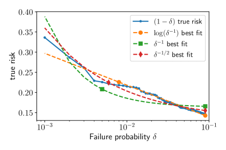
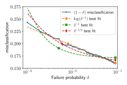
Figure 1: Dependence of the true risk and misclassification on the failure probability $\delta$, for a fixed number of samples and epochs. Our theory bounds the true risk by $O(1/\sqrt{\delta})$.

Figure 1 shows the dependence of the true risk and misclassification on the failure probability. For reference, we have also plotted the least-squares best fit of the data based on a $\log(1/\delta)$, $1/\delta$ and $1/\sqrt{\delta}$ form, allowing for an offset. We ignore data for $\delta>10^{-1}$ since we are interested in the limit $\delta\to 0$. However, the uncertainty does become greater as $\delta$ approaches $1/n_{\text{tri}}=10^{-3}$. For the true risk, the data are most consistent with a $\log(1/\delta)$ functional form, but not entirely inconsistent with $1/\sqrt{\delta}$. They do not appear to have a $1/\delta$ relationship. Our bound, which is of the $1/\sqrt{\delta}$ type, explains data much better than the naive bound using $1/\delta$. However, it is possible that stronger assumptions on the distribution could be used to improve the theoretical bound to reflect $\log(1/\delta)$ dependence. For the misclassification error, for which our experiment has no theoretical guarantees (since we trained with the surrogate loss), again we see that $\log(1/\delta)$ is most consistent with the data.

5.2 Non-convex Stochastic Approximation Convergence

Again let $\phi$ denote the ReLU function and consider

$$\forall x\in\mathbb{R}^{d_{1}},\quad h(\cdot\,;x):\mathbb{R}^{m\times d_{1}}\times\mathbb{R}^{m\times m}\times\mathbb{R}^{d_{2}\times m}\to\mathbb{R}^{d_{2}}:(A,B,C;x)\mapsto C\phi(B\phi(Ax))$$

and

$$\forall(x,y)\in\mathbb{R}^{d_{1}}\times\mathbb{R}^{d_{2}},\quad F(\cdot\,;x,y):\mathbb{R}^{m\times d_{1}}\times\mathbb{R}^{m\times m}\times\mathbb{R}^{d_{2}\times m}\to\mathbb{R}:(A,B,C;x,y)\mapsto\frac{1}{2}\|h(A,B,C;x)-y\|_{2}^{2}$$

By defining the matrices $D_{1}=D_{1}(A,x)=\text{diag}\mathbbm{I}_{Ax\geq 0}$ and $D_{2}=D_{2}(A,B,x)=\text{diag}\mathbbm{I}_{B\phi(Ax)\geq 0}$ we can rewrite $h$ and $F$ with matrices instead of ReLUs so that we can take the derivative. The gradients can be determined via automatic differentiation software like PyTorch, or, using Eq. (119) of Petersen and Pedersen (2008), we can work out the gradients by hand as follows:

$$\frac{\partial}{\partial A}F(A,B,C;x,y)=(CD_{2}BD_{1})^{\top}(CD_{2}BD_{1}Ax-y)x^{\top}$$

$$\frac{\partial}{\partial B}F(A,B,C;x,y)=(CD_{2})^{\top}(CD_{2}BD_{1}Ax-y)(D_{1}Ax)^{\top}$$

$$\frac{\partial}{\partial C}F(A,B,C;x,y)=(CD_{2}BD_{1}Ax-y)(D_{2}BD_{1}Ax)^{\top}.$$

Note that $A=B=C=0$ is a stationary point, so we should not initialize at zero.

Consider the stochastic approximation cost function

$$f(A,B,C)=\mathbb{E}_{x\sim U(S^{d_{1}-1})}[F(A,B,C;x,h^{\star}(A^{\star},B^{\star},C^{\star};x))],$$

where the inner dimension of $h^{\star}$ is $m^{\star}$.

We will apply SGD and compute the post-processing iterate via Eq. (14) with $n_{\text{iter}}$ test iterates and a test set of $n_{\text{test}}$ samples. We will compute the convergence error as the norm-squared of the empirical gradient over a validation set of $n_{\text{val}}$ samples. We will compare the convergence error of both the post-processing iterate and the last iterate. We expect the convergence error of the post-processing iterate to have a linear dependence on $\log(1/\delta)$ as long as $n_{\text{iter}}$, $n_{\text{test}}$, and $n_{\text{val}}$ are sufficiently large.

Consider input dimension $d_{1}=10$, output dimension $d_{2}=1$, true inner dimension $m^{\star}=20$, and model inner dimension $m=10$. Sample $A^{\star}_{ij}\sim N(0,2/m^{\star})$, $B^{\star}_{ij}\sim N(0,2/m^{\star})$, $C^{\star}_{ij}\sim N(0,1/d_{2})$, $(A_{0})_{ij}\sim N(0,2/m)$, $(B_{0})_{ij}\sim N(0,2/m)$, and $(C_{0})_{ij}\sim N(0,1/d_{2})$ in that order with numpy random seed 17. We use step-size $\eta_{t}=0.1/\sqrt{t+1}$, $T=1000$ iterations, batch-size $b=10$, and $n_{\text{tri}}=100$ trials. Finally, we set $n_{\text{iter}}=200$, $n_{\text{test}}=1000$, and $n_{\text{val}}=5000$.

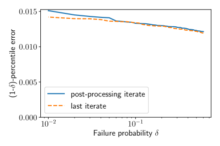
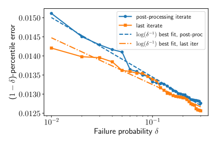
Figure 2: Top: Dependence of the convergence error on the failure probability. Bottom: Zoom, and line of best fit to $\log(1/\delta)$ form (allowing for an offset).

Figure 2 shows the $(1-\delta)$-percentile convergence error over the validation set, and the right plot shows a least-squares best fit line to the form $\log(1/\delta)$ (with an offset). As expected, the convergence error of the post-processing iterate depends linearly on $\log(1/\delta)$. The last iterate actually performs slightly better than the post-processing iterate even though it does not have the same theoretical guarantees; this justifies the standard practice of just using the last iterate.

5.3 Non-convex Sample Average Approximation Convergence

Here we modify the previous experiment by considering the sample average approximation cost function

$$f(A,B,C)=\frac{1}{n}\sum_{i=1}^{n}F(A,B,C;x_{i},h^{\star}(A^{\star},B^{\star},C^{\star};x_{i})).$$

Now, we actually do have access to the full gradient information for comparison if we are willing to pay the computational cost for a full batch gradient. This allows us to compare with the best iterate, computed via Eq. (12). Moreover, we can compute the convergence error as the norm-squared of the true gradient.

Again, consider input dimension $d_{1}=10$, output dimension $d_{2}=1$, true inner dimension $m^{\star}=20$, and model inner dimension $m=10$. Sample $A^{\star}_{ij}\sim N(0,2/m^{\star})$, $B^{\star}_{ij}\sim N(0,2/m^{\star})$, $C^{\star}_{ij}\sim N(0,1/d_{2})$, $(A_{0})_{ij}\sim N(0,2/m)$, $(B_{0})_{ij}\sim N(0,2/m)$, $(C_{0})_{ij}\sim N(0,1/d_{2})$, $X_{ij}\sim N(0,1)$ in that order with numpy random seed 17. Then normalize the rows of $X$ and compute $Y$. Again, we use step-size $\eta_{t}=0.1/\sqrt{t+1}$, $T=1000$ iterations, batch-size $b=10$, $n_{\text{tri}}=100$ trials, $n_{\text{iter}}=200$, and $n_{\text{test}}=1000$.

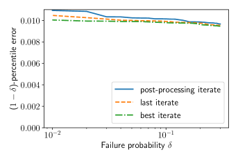
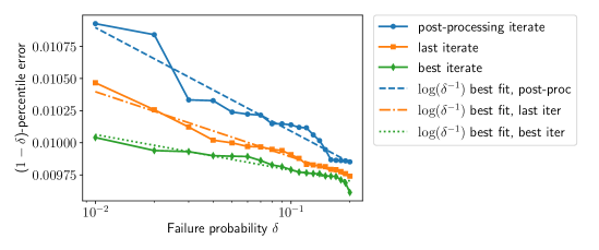
Figure 3: Top: Dependence of the convergence error on the failure probability. Bottom: Zoom, and line of best fit to $\log(1/\delta)$ form (allowing for an offset).

Figure 3 shows the $(1-\delta)$-percentile convergence error. The best iterate performs slightly better than the last iterate, and the last iterate performs slightly better than the post-processing iterate. The differences are slight, and all have a roughly $O(\log(1/\delta))$ relationship. Overall, this corroborates the theory: the iterate sampling scheme is slightly sub-optimal and scales similarly (in $\delta$) to the optimal iterate.

6 Conclusions

This paper analyzed the convergence of SGD for objective functions that satisfy the PL condition and for generic non-convex objectives. Under a sub-Gaussian assumption on the gradient error, we showed a high probability convergence rate matching the mean convergence rate for PL objectives. Our convergence result was then utilized in the context of statistical learning to support the practice of taking multiple but limited epochs of mini-batch SGD. Under a sub-Weibull assumption on the noise, we showed a high probability convergence rate matching the mean convergence rate for non-convex objectives. We also provided and analyzed a post-processing method for choosing a single iterate. To prove the convergence rate, we first proved a Freedman-type inequality for martingale difference sequences that extends previous Freedman-type inequalities beyond the sub-exponential threshold to allow for sub-Weibull tail-decay. Finally, we considered two synthetic neural net problems, one with a PL objective, and one with a non-convex objective. For the PL objective, we showed that the true risk and misclassification have high probability dependence on the failure probability. We leave improving our true risk bound to high probability and extending to classification as future work. For the non-convex objective, we showed that the convergence error has high probability dependence on the failure probability whether we choose the best iterate, the post-processing iterate, or the last iterate.

Appendix A Standard Optimization Results

We state a few useful definitions and results from optimization. More details can be found in Nesterov (2018) and Bubeck (2015). All our definitions are with respect to the Euclidean norm, denoted $\|\cdot\|$, and we let $f:\mathbb{R}^{d}\rightarrow\mathbb{R}$. We write $C^{1}(\mathbb{R}^{d})$ or just $C^{1}$ to denote functionals on $\mathbb{R}^{d}$ that are continuously differentiable.

Definition 14 (Lipschitz continuity).

We say $f:\mathbb{R}^{d}\rightarrow\mathbb{R}$ is $\rho$-Lipschitz continuous if $|f(x)-f(y)|\leq\rho\|x-y\|$ for all $x,y\in\mathbb{R}^{d}$. Likewise, $g:\mathbb{R}^{d}\rightarrow\mathbb{R}^{m}$ is $\rho$-Lipschitz continuous if $\|g(x)-g(y)\|\leq\rho\|x-y\|$ for all $x,y\in\mathbb{R}^{d}$.

Note that averages of Lipschitz continuous functions are Lipschitz continuous with the same constant by the triangle inequality. Also, if $f\in C^{1}$, then $f$ is $\rho$-Lipschitz if and only if $\|\nabla f(x)\|\leq\rho$ for all $x\in\mathbb{R}^{d}$.

Definition 15 (L-smoothness).

We say $f$ is $L$-smooth if $f\in C^{1}$ and its gradient is $L$-Lipschitz continuous.

If $f$ is $L$-smooth, then a standard result is

$$(\forall x,y\in\mathbb{R}^{d})\;f(y)\leq f(x)+\langle\nabla f(x),y-x\rangle+\frac{L}{2}\|x-y\|^{2}.$$ (15)

Applying this result to $x-\frac{1}{L}\nabla f(x)$ and $x$ and rearranging terms gives

$$\|\nabla f(x)\|^{2}\leq 2L(f(x)-f^{\star})$$ (16)

and taking $x\in\text{argmin}_{x^{\prime}}\,f(x^{\prime})$ gives

$$f(y)-f^{\star}\leq\frac{L}{2}\|y-x^{\star}\|^{2}.$$

If $f$ is both $\mu$-PL and $L$-smooth, then combining the PL inequality and Eq. (16) gives

$$f(x)-f^{\star}\leq\frac{L}{\mu}\left(f(x)-f^{\star}\right)$$

which implies $L\geq\mu$.

The following inequality is known as the quadratic growth (QG) condition:

$$\exists\mu>0\quad\text{s.t. }(\forall x\in\mathbb{R}^{d})\;\|x-\mathcal{P}_{X^{\star}}(x)\|\leq\frac{2}{\mu}\left(f(x)-f^{\star}\right)$$ (17)

where $\mathcal{P}_{X^{\star}}$ denotes the (set-valued) Euclidean projection onto the set of global minimizers, $X^{\star}=\text{argmin}_{x}\,f(x)$. The PL inequality implies the QG condition (Karimi et al, 2016).

Strong convexity implies the PL inequality but the PL inequality only implies invexity, not convexity. Furthermore, unlike the convexity and strong convexity properties, the PL property is not preserved under nonnegative sums. The PL inequality implies the quadratic growth property (Eq. 17), which can be used to bound how far away the nearest minimizer is in terms of the optimality gap (which can be bounded above by simply evaluating the cost function, if the cost function is nonnegative).

Appendix B Convergence of Random Variables

See (Billingsley, 1995, Sec. 20) for details. A sequence of random variables $X_{t}$ converges to $X$ :

• in probability if, for all $\epsilon>0$, $\lim_{t}P(|X_{t}-X|>\epsilon)=0$, denoted $X_{t}\overset{p}{\to}X$;

• in mean if $\lim_{t}\mathbb{E}|X_{t}-X|=0$, denoted $X_{t}\overset{L^{1}}{\to}X$;

• almost surely if $P(\lim_{t}X_{t}=X)=1$, denoted $X_{t}\overset{a.s.}{\to}X$.

When the rate of convergence is of interest, we say a sequence of random variables $X_{t}$ converges to $X$:

• with mean convergence rate $r(t)$ if, for all $t$, $\mathbb{E}|X_{t}-X|\leq r(t)$;

• with convergence rate $\tilde{r}(t,\delta)$ if, for all $t$ and $\delta$, $P\left(|X_{t}-X|\leq\tilde{r}(t,\delta)\,\right)\geq 1-\delta$.

In particular, when $\tilde{r}(t,\delta)$ is separable, i.e. $\tilde{r}(t,\delta)=r(t)p(\delta)$, we use “high probability” to refer to $p(\delta)=\text{poly}(\log(1/\delta))$ and “low probability” to refer to $p(\delta)=\text{poly}(1/\delta)$. All five kinds of convergence are interrelated:

• Convergence in mean and convergence almost surely both imply convergence in probability.

• Mean convergence with rate $r(t)$ such that $r(t)\to 0$ as $t\to\infty$ implies convergence in mean.

• By Markov’s inequality, mean convergence with rate $r(t)$ implies convergence with rate $r(t)/\delta$.

• By the Borel-Cantelli lemma (Billingsley, 1995, Thm. 4.3), convergence with rate $r(t)p(\delta)$ implies almost sure convergence if $\sum_{t=0}^{\infty}\min\{1,p^{-1}(a/r(t))\}<\infty$ for all $a>0$. If $p(\delta)=1/\delta^{c}$ for some $c>0$, then $r(t)=o(1/t^{c})$ is required. If $p(\delta)=\log(1/\delta)$, then only $r(t)=O(1/t^{c})$ for some $c>0$ is required.

Appendix C Proof of Proposition 5

We want to find requirements on a sequence $(K_{i})$ such that $\mathbb{E}\left[\exp(\lambda X_{i})\right]\leq\exp(\lambda K_{i})\leavevmode\nobreak\ \forall\lambda\in[0,K_{i}^{-1}]$. Then, by Markov’s inequality and taking $\lambda_{n}=K_{n}^{-1}$, $P\left(X_{n}\geq\log(e/\delta)K_{n}\right)=P\left(\exp(X_{n}/K_{n})\geq e/\delta\right)\leq\delta$. Our proof is inductive. For the base case, we need

$$(1)\leavevmode\nobreak\ K_{0}\geq X_{0}.$$

For the induction step, assume $\mathbb{E}\left[\exp(\tilde{\lambda}X_{i})\right]\leq\exp(\tilde{\lambda}K_{i})\leavevmode\nobreak\ \forall\tilde{\lambda}\in[0,K_{i}^{-1}]$. Let $\lambda\in[0,K_{i+1}^{-1}]$. Then

$$\mathbb{E}\left[\exp(\lambda X_{i+1})\right] \leq\mathbb{E}\left[\exp(\lambda\alpha_{i}X_{i}+\lambda\hat{w}_{i}+\lambda\hat{v}_{i})\right]\quad\text{by non-negativity}$$

$$\overset{\text{TE}}{=}\mathbb{E}\left[\exp(\lambda\alpha_{i}X_{i})\mathbb{E}\left[\exp(\lambda\hat{w}_{i})\exp(\lambda\hat{v}_{i})\mid\mathcal{F}_{i-1}\right]\right]$$

$$\overset{\text{CS}}{\leq}\mathbb{E}\left[\exp(\lambda\alpha_{i}X_{i})\mathbb{E}\left[\exp(2\lambda\hat{w}_{i})\mid\mathcal{F}_{i-1}\right]^{1/2}\mathbb{E}\left[\exp(2\lambda\hat{v}_{i})\mid\mathcal{F}_{i-1}\right]^{1/2}\right]$$

$$\overset{(2)}{\leq}\mathbb{E}\left[\exp(\lambda\alpha_{i}X_{i})\exp\left(\frac{(2\lambda)^{2}}{2}\beta_{i}^{2}X_{i}\right)^{1/2}\exp(2\lambda\gamma_{i})^{1/2}\right]\quad\text{if}\quad 2\lambda\in[0,\gamma_{i}^{-1}]$$

$$=\mathbb{E}\left[\exp(\lambda\alpha_{i}X_{i}+\lambda^{2}\beta_{i}^{2}X_{i}+\lambda\gamma_{i})\right]$$

$$=\mathbb{E}\left[\exp(\lambda(\alpha_{i}+\lambda\beta_{i}^{2})X_{i}\right]\exp(\lambda\gamma_{i})$$

$$\overset{(3)}{\leq}\exp(\lambda((\alpha_{i}+\lambda\beta_{i}^{2})K_{i}+\gamma_{i}))\quad\text{via induction if}\;\tilde{\lambda}:=\lambda(\alpha_{i}+\lambda\beta_{i}^{2})\leq K_{i}^{-1}$$

$$\overset{(4)}{\leq}\exp(\lambda K_{i+1})$$

where $TE$ denotes the law of total expectation (Billingsley, 1995, Thm. 34.3), $CS$ denotes the Cauchy-Schwarz inequality, and $(2)-(4)$ are the requirements

$$(2)\leavevmode\nobreak\ 2\lambda\leq\gamma_{i}^{-1}\impliedby 2K_{i+1}^{-1}\leq\gamma_{i}^{-1}\iff K_{i+1}\geq 2\gamma_{i}$$

$$(3)\leavevmode\nobreak\ \lambda(\alpha_{i}+\lambda\beta_{i}^{2})\leq K_{i}^{-1}\impliedby K_{i+1}^{-1}(\alpha_{i}+K_{i+1}^{-1}\beta_{i}^{2})\leq K_{i}^{-1}\iff K_{i+1}^{2}\geq\alpha_{i}K_{i}K_{i+1}+\beta_{i}^{2}K_{i}$$

$$(4)\leavevmode\nobreak\ K_{i+1}\geq(\alpha_{i}+\lambda\beta_{i}^{2})K_{i}+\gamma_{i}\impliedby K_{i+1}\geq(\alpha_{i}+K_{i+1}^{-1}\beta_{i}^{2})K_{i}+\gamma_{i}\iff K_{i+1}^{2}\geq(\alpha_{i}K_{i}+\gamma_{i})K_{i+1}+\beta_{i}^{2}K_{i}.$$

The requirement of the proposition implies requirements $(2)-(4)$, completing the proof.

Appendix D Proof of Theorem 6

We first note that $\eta_{t}$ is decreasing in $t$ for $\kappa\geq 1$ and $t\geq 0$, and so

$$\eta_{t}=\frac{2t+4\kappa-1}{\mu(t+2\kappa)^{2}}\leq\frac{4\kappa-1}{\mu(2\kappa)^{2}}\leq\frac{4\kappa}{\mu 4\kappa^{2}}=\frac{1}{L}\,.$$

Thus, we can use Eq. (3):

$$f(x_{t+1})-f^{\star}\leq(1-\mu\eta_{t})(f(x_{t})-f^{\star})+\eta_{t}(1-L\eta_{t})\langle\nabla f(x_{t}),e_{t}\rangle+\frac{L\eta_{t}^{2}}{2}\|e_{t}\|^{2}.$$ (18)

Defining

$$X_{t}=(t+2\kappa-1)^{2}(f(x_{t})-f^{\star})$$

$$\hat{w}_{t}=\eta_{t}(1-L\eta_{t})(t+2\kappa)^{2}\langle\nabla f(x_{t}),e_{t}\rangle$$

$$\hat{v}_{t}=\frac{L\eta_{t}^{2}(t+2\kappa)^{2}}{2}\|e_{t}\|^{2}$$

then multiplying both sides of Eq. (18) by $(t+2\kappa)^{2}$ and noting $1-\mu\eta_{t}=\frac{(t+2\kappa-1)^{2}}{(t+2\kappa)^{2}}$ gives the recursion

$$X_{t+1}\leq X_{t}+\hat{w}_{t}+\hat{v}_{t}.$$

Observe that

$$\mathbb{E}\left[\exp\left(\frac{\hat{w}_{t}^{2}}{\frac{18L}{\mu^{2}}X_{t}\sigma^{2}}\right)\bigg{|}\leavevmode\nobreak\ \mathcal{F}_{t-1}\right] \leq\mathbb{E}\left[\exp\left(\frac{\eta_{t}^{2}(1-L\eta_{t})^{2}(t+2\kappa)^{4}\|\nabla f(x_{t})\|^{2}\|e_{t}\|^{2}}{\frac{18L}{\mu^{2}}X_{t}\sigma^{2}}\right)\bigg{|}\leavevmode\nobreak\ \mathcal{F}_{t-1}\right]$$

$$\leq\mathbb{E}\left[\exp\left(\frac{\eta_{t}^{2}(1-L\eta_{t})^{2}\frac{(t+2\kappa)^{4}}{(t+2\kappa-1)^{2}}2LX_{t}\|e_{t}\|^{2}}{\frac{18L}{\mu^{2}}X_{t}\sigma^{2}}\right)\bigg{|}\leavevmode\nobreak\ \mathcal{F}_{t-1}\right]\quad\text{via }\eqref{eq:LipschitzBound}$$

$$\leq\mathbb{E}\left[\exp\left(\frac{\frac{18L}{\mu^{2}}X_{t}\|e_{t}\|^{2}}{\frac{18L}{\mu^{2}}X_{t}\sigma^{2}}\right)\bigg{|}\leavevmode\nobreak\ \mathcal{F}_{t-1}\right]$$

$$\leq 2$$

since $\|e_{t}\|$ is assumed to be $\sigma$-sub-Gaussian. Similarly,

$$\mathbb{E}\left[\exp\left(\frac{\hat{v}_{t}}{\frac{2L}{\mu^{2}}\sigma^{2}}\right)\bigg{|}\leavevmode\nobreak\ \mathcal{F}_{t-1}\right] \leq\mathbb{E}\left[\exp\left(\frac{\frac{2L}{\mu^{2}}\|e_{t}\|^{2}}{\frac{2L}{\mu^{2}}\sigma^{2}}\right)\bigg{|}\leavevmode\nobreak\ \mathcal{F}_{t-1}\right]$$

$$\leq 2.$$

Thus, conditioned on $\mathcal{F}_{t-1}$, $\hat{w}_{t}$ is centered and $\frac{18L}{\mu^{2}}X_{t}\sigma^{2}$-sub-Gaussian and $\hat{v}_{t}$ is $\frac{2L}{\mu^{2}}\sigma^{2}$-sub-exponential. Thus, for absolute constants $a$ and $b$, by Prop. 2.5.2 and Prop. 2.7.1 of Vershynin (2018), we can set $\beta_{t}^{2}=\frac{18aL\sigma^{2}}{\mu^{2}}$ and $\gamma_{t}=\frac{2bL\sigma^{2}}{\mu^{2}}$ and use Proposition 5. In particular, we can set

$$K_{T} =X_{0}+\sum_{t=0}^{T-1}(2\gamma_{t}+\beta_{t}^{2})$$

$$=X_{0}+\frac{(18a+2b)L\sigma^{2}T}{\mu^{2}}.$$

Dividing by $(T+2\kappa)^{2}$ completes the proof.

Appendix E PL Projected SGD

When working with constraints to a set $x\in X\subsetneq\mathbb{R}^{d}$, if $f$ is strongly convex, then so is $f$ added to the indicator function of $X$, and results for gradient descent methods easily extend to projected gradient descent. On the other hand, if $f$ is PL, then $f$ plus the indicator function is not KL (Kurdyka-Łojasiewicz). This has real impacts on gradient descent algorithms, where gradient descent might converge but projected gradient descent does not. For example, there is a smooth function, a mollified version of $f(x,y)=\left(a(x)_{+}^{2}-b\left(|y|-c\right)_{+}\right)_{+}$, such that the PL inequality is satisfied but projected gradient descent does not converge to a minimizer; we formalize this in the remark below.

Remark 16.

Consider $f(x,y)=\left(a(x)_{+}^{2}-b\left(|y|-c\right)_{+}\right)_{+}$ where $(\cdot)_{+}$ denotes $\max(\cdot,0)$ and $a,b>0,c\geq 0$. The minimum of $f$ is 0 and $X^{\star}=\{(x,y)\leavevmode\nobreak\ |\leavevmode\nobreak\ x\leq 0\text{ or }|y|\geq\frac{a}{b}x^{2}+c\}$. If we use $\varphi(x)=\mathcal{X}_{B_{1}(0)}\cdot\exp\left(-1/(1-\|x\|^{2})\right)/\Phi$—where $\mathcal{X}$ denotes the indicator function, $B_{1}(0)$ denotes the ball of radius 1 centered at 0, and $\Phi$ is the normalization constant—to mollify $f$, then, for $\epsilon<c$, $f_{\epsilon}$ has PL constant $2a$ and smoothness constant $2a$. Consider the starting point $(d,0)$. For $a,b,c,d$ chosen appropriately, the distance from $(d,0)$ to its projection onto $X^{\star}$ is strictly less than $d$. Thus, if we let $X$ be the ball centered at $(d,0)$ with radius equal to exactly that distance, then the constrained problem and the unconstrained problem have the same minimum. However, projected gradient flow, starting from $(d,0)$, ends up stuck at a non-minimizer: the point of $X$ closest to $(0,0)$. See Figure 4 for the contour plot when $a=1/10$, $b=1=c$, and $d=10$.

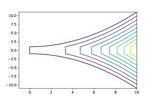
Figure 4: Contour plot of the PL function counter-example to projected gradient flow

In order to generalize gradient methods to projected gradient methods under PL-like assumptions, the proper generalization is that the function should satisfy a proximal PL inequality (Karimi et al, 2016). However, such an assumption is quite restrictive compared to the PL inequality. We leave the problem of convergence with just the PL inequality, via added noise or a Frank-Wolfe type construction, as a future research direction.

Appendix F Generalization Results

A random vector $X$ is $\sigma$-sub-Gaussian if $\langle u,X\rangle$ is $\sigma$-sub-gaussian for all unit vectors $u$ (Vershynin, 2018, Def. 3.4.1). Assume $\nabla f(x)-g(x,1)$ is $\sigma/\sqrt{d}$-sub-Gaussian. Then $\nabla f(x)-g(x,b)$ is $C\sigma/\sqrt{bd}$-sub-Gaussian for some universal constant $C$ by Hoeffding’s inequality (Vershynin, 2018, Prop. 2.6.1). Furthmore, by Lemma 1 of Jin et al (2019), $\|\nabla f(x)-g(x,1)\|$ is $C\sigma/\sqrt{b}$-sub-Gaussian. So, $\|\nabla f(x)-g(x,1)\|^{2}$ is $C^{2}\sigma^{2}/b$-sub-exponential.

Definition 17.

Let $S$ and $S^{\prime}$ differ in at most one sample. Let $g$ and $g^{\prime}$ be the respective gradient estimators. Define $x_{0}=x_{0}^{\prime}$ and, for $t\geq 0$, $x_{t+1}=x_{t}-\eta_{t}g(x_{t},b_{t})$ and $x_{t+1}^{\prime}=x_{t}^{\prime}-\eta_{t}g^{\prime}(x_{t}^{\prime},b_{t})$. We say SGD with $T$ iterations is $\alpha$-uniformly stable in expectation if for all $S$ and $S^{\prime}$, $\sup_{s}|\mathbb{E}[\ell(x_{T},s)-\ell(x_{T}^{\prime},s)]|\leq\alpha$.

Theorem 18.

(Elisseeff et al, 2005, Thm. 12) Assume $\ell(x,s)\in[0,M]$ for all $x$ and $s$. Let $\delta\in(0,1)$. If SGD with $T$ steps is $\alpha$-uniformly stable in expectation then, $\text{w.p.}\geq 1-\delta$ over $S$ and $(i_{t})$ for all SGD,

$$\tilde{f}(x_{T})-f(x_{T}) \leq\sqrt{\frac{6Mn\alpha+M^{2}}{2n\delta}}.$$

Note that Thm. 12 of Elisseeff et al (2005) is actually for pointwise hypothesis stability in expectation, but uniform stability in expectation implies pointwise hypothesis stability in expectation. Furthermore, in the form we have it, Theorem 18 can be proved using Lem. 9 of Bousquet and Elisseeff (2002) and Chebyshev’s inequality.

Define $\delta_{t}\coloneqq\|x_{t}-x_{t}^{\prime}\|$. Note that $P(I_{t}=I_{t}^{\prime})=\left(1-\frac{1}{n}\right)\cdots\left(1-\frac{1}{n-b_{t}+1}\right)=1-\frac{b_{t}}{n}$. Following Hardt et al (2016), a uniform stability bound is sought by bounding the growth of $\delta_{t}$; if $\ell(\cdot,s)$ is $\rho$-Lipschitz, this implies that $\sup_{s}|\ell(x_{t},s)-\ell(x_{t}^{\prime},s)|\leq\rho\delta_{t}$.

Lemma 19.

(Hardt et al, 2016, Lem. 2.5) Assume $\ell(\cdot,s)$ is $\rho$-Lipschitz and $L$-smooth for all $s$. Then,

$$\delta_{t+1} \leq\begin{cases}(1+\eta_{t}L)\delta_{t}&\text{ if }I_{t}=I_{t}^{\prime}\\ \delta_{t}+2\eta_{t}\rho&\text{ o.w.}\end{cases}.$$

Theorem 20.

Let $\eta_{t}\leq c/(t+1)$ and $b_{t}=b$. Assume $\ell(\cdot,s)$ is $\rho$-Lipschitz and $L$-smooth for all $s$. Then, SGD with $T$ iterations is $\alpha$-uniformly stable in expectation with

$$\alpha\leq\frac{2\rho^{2}T^{Lc}(c+1/L)b}{n}.$$

Proof.

Define $a_{t}=0$ if $I_{t}=I_{t}^{\prime}$ and $a_{t}=1$ otherwise. Hence, $a_{t}\sim B(1,p)$ independently with $p=b/n$. By Lemma 19,

$$\delta_{t+1} \leq(1+(1-a_{t})\eta_{t}L)\delta_{t}+2\eta_{t}\rho a_{t}$$

$$\leq(1+\eta_{t}L)\delta_{t}+2\eta_{t}\rho a_{t}.$$

Thus,

$$\delta_{T} \leq 2\rho\sum_{t=0}^{T-1}\prod_{i=t+1}^{T-1}(1+\eta_{i}L)\eta_{t}a_{t}$$

$$\leq 2\rho\sum_{t=0}^{T-1}\exp\left(L\sum_{i=t+1}^{T-1}\eta_{i}\right)\eta_{t}a_{t}$$

$$\leq 2\rho c\sum_{t=0}^{T-1}\exp\left(Lc\log\left(\frac{T}{t+1}\right)\right)\frac{a_{t}}{t+1}$$

$$\leq 2\rho cT^{Lc}\sum_{t=0}^{T-1}\frac{a_{t}}{(t+1)^{Lc+1}}.$$

Note that

$$\sum_{t=0}^{T-1}\frac{1}{(t+1)^{Lc+1}} \leq 1+\int_{0}^{T-1}\frac{dt}{(t+1)^{Lc+1}}$$

$$=1+\frac{1}{Lc}-\frac{1}{LcT^{Lc}}$$

$$\leq 1+\frac{1}{Lc}.$$

The result follows by taking expectation and using $\sup_{s}|\ell(x_{t},s)-\ell(x_{t}^{\prime},s)|\leq\rho\delta_{t}$. ∎

Thm. 20 is essentially Thm. 3.12 of Hardt et al (2016). In fact, the two theorems consist of the same analysis with only two differences. First, we extend the analysis to mini-batch SGD, though this extension is not difficult. Second, Hardt et al (2016) consider the first iteration where instability becomes non-zero. They use this to break up the bound and optimize over it. However, in so doing, they introduce the restriction $(2cL)^{1/(Lc+1)}T^{Lc/(Lc+1)}<n$. Thus, for simplicity, we left out this step. While it seems that makes our bound significantly larger, that is only when the restriction is not met (in which case their bound is vacuous).

To prove Theorem 9, we follow similar steps to Appendix D but set

$$X_{t}=(t+1)^{\mu c}\left(f(x_{t})-f^{\star}\right)$$

$$\hat{w}_{t}=\eta(1-L\eta_{t})(t+2)^{\mu c}\langle\nabla f(x_{t}),e_{t}\rangle$$

$$\hat{v}_{t}=\frac{L\eta_{t}^{2}(t+2)^{\mu c}}{2}\|e_{t}\|^{2}$$

and find that, conditioned on $\mathcal{F}_{t-1}$, $\hat{w}_{t}$ is centered and $\frac{6Lc^{2}}{(t+1)^{2-\mu c}}X_{t}\sigma^{2}$-sub-Gaussian and $\hat{v}_{t}$ is $\frac{Lc^{2}}{(t+1)^{2-\mu c}}\sigma^{2}$-sub-exponential. So, we can set

$$K_{T}=O\left(X_{0}+\frac{Lc^{2}\sigma^{2}}{b}\right).$$

Dividing by $(T+1)^{\mu c}$ completes the proof.

Finally, note that the assumptions for generalization are interrelated with the assumptions for convergence:

Proposition 21.

Define $f$ as in Eq. (4) and assume it is $\mu$-PL. Assume $\ell(\cdot,s)$ is $L$-smooth for all $s$. Then $f$ is $L$-smooth. Moreover, if $\nabla f(x)-g(x,1)$ is sub-gaussian and $\ell(x,s)$ is nonnegative for all $x$ and $s$, and assuming interpolation ($f^{\star}=0$), then for $(x_{t})$ generated by SGD with a $\mathcal{O}(1/t)$ step-size sequence there exists a constant $R<\infty$ such that $P\left(\|x_{t}-x_{0}\|\leq R\leavevmode\nobreak\ \forall t\in\mathbb{N}\right)=1$. If $s$ comes from a compact set (e.g., normalized data) and we assume $\ell(x,s)$ is jointly continuous in $x$ and $s$, then there exist constants $\rho$ and $M$ such that, for all $x$ in the ball of radius $R$ around $x_{0}$ and for all $s$, $\ell(x,s)$ is $\rho$-Lipschitz with respect to $x$ and is bounded above by $M$.

Proof.

The smoothness of $f$ easily follows from that of $\ell$ using the definition of $f$ in Eq. (4), the definition of smoothness, and the triangle inequality.

The rest of the proof will hinge on bounding the SGD sequence $(x_{t})$. Unrolling the SGD updates, we have $x_{T+1}=x_{0}+\sum_{t=0}^{T}\eta_{t}g_{t}$. Define $\tilde{f}_{t}=\frac{1}{b_{t}}\sum_{i\in I_{t}}\ell(\cdot,s_{i})$ so that $g(\cdot,b_{t})=\nabla\tilde{f}_{t}$, and observe $\tilde{f}$ is $L$-smooth for the same reason that $f$ is $L$-smooth. Then,

$$\|g(x,b_{t})\|^{2}=\|\nabla\tilde{f}_{t}(x)\|^{2} \leq 2L(\tilde{f}_{t}(x)-\tilde{f}_{t}^{\star})$$

$$\leq 2L\tilde{f}_{t}(x)$$

$$\leq 2L\frac{n}{b_{t}}f(x)$$

where the first inequality follows from Eq. (16), the second from nonnegativity, and the third from nonnegativity as well. For simplicity, assume a fixed minibatch size $b_{t}=b$.

Thus, by the triangle inequality, $\|x_{T}-x_{0}\|\leq\sqrt{2L\frac{n}{b}}\sum_{t=0}^{T-1}\eta_{t}\sqrt{f(x_{t})}$. For both Thm. 6 and Thm. 9, the step-size is $\eta_{t}=\mathcal{O}(1/t)$, and, by interpolation, $f(x_{t})\leq\log(1/\delta_{t})\frac{C}{t^{c}}$ for each $t$ with probability $1-\delta_{t}$, where $C$ and $c>0$ are constants (e.g., $c=1$ for Thm. 6). Choose $\delta_{t}=\mathcal{O}(1/t^{2})$, then it holds that

$$\text{w.p.}\geq 1-\delta,\quad(\forall T\in\mathbb{N})\quad\|x_{T}-x_{0}\|\lesssim C^{\prime}\sum_{t=1}^{T}\frac{\log(t)}{t^{1+c/2}}\leq C^{\prime\prime}$$

for constants $C^{\prime}$ and $C^{\prime\prime}$ since the series converges (verified by, e.g., the integral test) and with $\delta=\sum_{t=0}^{T-1}\delta_{t}\leq\sum_{t=0}^{\infty}\delta_{t}<1$ coming from the union bound and the fact $\sum_{t=1}^{\infty}t^{-2}=\pi^{2}/6<\infty$.

Let $E_{k}$ be the event that $\|x_{T}-x_{0}\|\leq k$ for all $T$. Then the event $\bigcup_{k=1}^{\infty}E_{k}$ implies that $(x_{t})_{t=0}^{\infty}$ is a bounded sequence. Since $E_{k}$ is nested, by continuity of measure, $P(\bigcup_{k=1}^{\infty}E_{k})=\lim_{k\rightarrow\infty}P(E_{k})$, and the argument from the previous paragraph shows that $P(E_{k})$ can be made arbitrarily close to $1$ by choosing a sufficiently large radius $k$. Hence $(x_{t})_{t=0}^{\infty}$ is a bounded sequence with probability $1$.

Now that $(x_{t})$ is bounded with probability $1$, we turn to $\rho$ and $M$. First, $\ell(x,s)$ is jointly continuous in $x$ and $s$, and since $(x,s)$ comes from a compact set, we get that $\ell$ attains its maximum value (Hunter and Nachtergaele, 2001, Thm. 1.68), which we call $M$. The same is true of $\|\nabla_{x}\ell(x,s)\|$ and we call its maximum value $\rho$. Thus, since $\ell(x,s)$ is $C^{1}$ with respect to $x$, we have that it is $\rho$-Lipschitz with respect to $x$. ∎

Appendix G Sub-Weibull Properties

Lemma 22 provides a simple bound for $\mathbb{E}\left[|X|^{p}\right]$; the proof is included for completeness and to demonstrate the techniques. Lemma 23 is from Prop. 2.5.2 of Vershynin (2018). Lemma 24 extends Prop. 2.7.1 of Vershynin (2018) to interpolate between the sub-Gaussian and sub-exponential regimes. Lemma 25 is an application of Thm. 1 of Vladimirova et al (2020), Lma. 5 of Wong et al (2020), and the triangle inequality for $L_{p}$ spaces (note that this is called the Minkowski inequality and requires $p\geq 1$).

To go from probability to expectation, the CDF formula is used:

$$\mathbb{E}\left[|Y|\right]=\int_{0}^{\infty}P\left(|Y|>t\right)dt.$$

To go from expectation to probability, Markov’s inequality is used:

$$P\left(|Y|>t\right)\leq\frac{1}{t}\mathbb{E}\left[|Y|\right]\leavevmode\nobreak\ \forall t>0.$$

In both cases, the trick is choosing what $Y$ should be, e.g. $Y=|X|^{p}$ or $Y=\exp((\lambda|X|)^{1/\theta})$.

Lemma 22.

If $X$ is $K$-sub-Weibull($\theta$) then $\mathbb{E}\left[|X|^{p}\right]\leq 2\Gamma(\theta p+1)K^{p}\leavevmode\nobreak\ \forall p>0$. In particular, $\mathbb{E}\left[X^{2}\right]\leq 2\Gamma(2\theta+1)K^{2}$.

Proof.

First, for all $t\geq 0$,

$$P\left(|X|\geq t\right) =P\left(\exp\left(\left(|X|/K\right)^{1/\theta}\right)\geq\exp\left(\left(t/K\right)^{1/\theta}\right)\right)$$

$$\leq 2\exp\left(-\left(t/K\right)^{1/\theta}\right).$$

Second,

$$\mathbb{E}\left[|X|^{p}\right] =\int_{0}^{\infty}P\left(|X|^{p}\geq x\right)dx$$

$$\leq 2\int_{0}^{\infty}\exp\left(-\left(x^{1/p}/K\right)^{1/\theta}\right)$$

$$=2\theta pK^{p}\int_{0}^{\infty}\exp(-u)u^{\theta p-1}du$$

$$=2\theta p\Gamma(\theta p)K^{p}$$

$$=2\Gamma(\theta p+1)K^{p}.$$

∎

Lemma 23.

(Vershynin, 2018, Prop. 2.5.2(e)) If $X$ is centered and $K$-sub-Guassian then $\mathbb{E}\left[\exp(\lambda X)\right]\leq\exp(\lambda^{2}K^{2})\leavevmode\nobreak\ \forall\lambda\in\mathbb{R}$.

Lemma 24.

If $X$ is centered and $K$-sub-Weibull($\theta$) with $\theta\in(1/2,1]$, then
$\mathbb{E}\left[\exp(\lambda X)\right]\leq\exp\left(\frac{\lambda^{2}}{2}(4\theta)^{2\theta}e^{2}K^{2}\right)$ for all $\lambda\in\left[0,\frac{1}{(4\theta)^{\theta}eK}\right]$.

Proof.

First, using Lemma 22 and $\Gamma(x+1)\leq x^{x}\leavevmode\nobreak\ \forall x\geq 1$, we can get $\|X\|_{p}\leq(2\theta)^{\theta}Kp^{\theta}$ for all $p\geq 1/\theta$, and so, in particular, for all $p\geq 2$. Thus, if $\lambda\in\left[0,\frac{1}{(4\theta)^{\theta}eK}\right]$, then

$$\mathbb{E}\left[\exp(\lambda X)\right] =\mathbb{E}\left[1+\lambda X+\sum_{p=2}^{\infty}\frac{(\lambda X)^{p}}{p!}\right]$$

$$=1+\sum_{p=2}^{\infty}\frac{\lambda^{p}\|X\|_{p}^{p}}{p!}$$

$$\leq 1+\sum_{p=2}^{\infty}\frac{\lambda^{p}(2\theta)^{\theta p}K^{p}p^{\theta p}}{p!}$$

$$\leq 1+\sum_{p=2}^{\infty}\left(\frac{\lambda(2\theta)^{\theta}eK}{p^{1-\theta}}\right)^{p}$$

$$\leq 1+\sum_{p=2}^{\infty}\left(\lambda(4\theta)^{\theta}(e/2)K\right)^{p}$$

$$\leq 1+\frac{\left(\lambda(4\theta)^{\theta}(e/2)K\right)^{2}}{1-\lambda(4\theta)^{\theta}(e/2)K}$$

$$\leq 1+2\left(\lambda(4\theta)^{\theta}(e/2)K\right)^{2}$$

$$\leq\exp\left(\frac{\lambda^{2}}{2}(4\theta)^{2\theta}e^{2}K^{2}\right),$$

completing the proof. ∎

Lemma 25.

(Vladimirova et al, 2020, Thm. 1) (Wong et al, 2020, Lma. 5) Suppose $X_{1},\ldots,X_{n}$ are sub-Weibull$(\theta)$ with respective parameters $K_{1},\ldots,K_{n}$. Then, for all $t\geq 0$,

$$P\left(\bigg{|}\sum_{i=1}^{n}X_{i}\bigg{|}\geq t\right)\leq 2\exp\left(-\left(\frac{t}{v(\theta)\sum_{i=1}^{n}K_{i}}\right)^{1/\theta}\right),$$

where $v(\theta)=(4e)^{\theta}$ for $\theta\leq 1$ and $v(\theta)=2(2e\theta)^{\theta}$ for $\theta\geq 1$.

Appendix H Proof of Proposition 11

The novel lemmas used in the proof are Lemma 27 and Lemma 31.

Observe that:

$$P\left(|\xi_{i}|\geq t\mid\mathcal{F}_{i-1}\right) =P\left(\exp\left((|\xi_{i}|/K_{i-1})^{1/\theta}\right)\geq\exp\left((t/K_{i-1})^{1/\theta}\right)\mid\mathcal{F}_{i-1}\right)$$

$$\leq 2\exp\left(-(t/K_{i-1})^{1/\theta}\right).$$

Moreover, observe that:

$$P\left(|\xi_{i}|\geq cK_{i-1}\right) =P\left(\exp\left((|\xi_{i}|/K_{i-1})^{1/\theta}\right)\geq\exp\left(c^{1/\theta}\right)\right)$$

$$\leq\exp\left(-c^{1/\theta}\right)\mathbb{E}\left[\exp\left((|\xi_{i}|/K_{i-1})^{1/\theta}\right)\right]$$

$$=\exp\left(-c^{1/\theta}\right)\mathbb{E}\left[\mathbb{E}\left[\exp\left((|\xi_{i}|/K_{i-1})^{1/\theta}\right)\mid\mathcal{F}_{i-1}\right]\right]$$

$$\leq 2\exp\left(-c^{1/\theta}\right).$$

We call the first result tail bound 1:

$$P\left(|\xi_{i}|\geq t\mid\mathcal{F}_{i-1}\right)\leq 2\exp\left(-(t/K_{i-1})^{1/\theta}\right)$$ (TB1)

and the second result tail bound 2:

$$P\left(|\xi_{i}|\geq cK_{i-1}\right)\leq 2\exp\left(-c^{1/\theta}\right)$$ (TB2)

The following lemma is not novel, but distills the proof technique of Freedman (1975), as found in the proof of Thm. 2.1 of Fan et al (2015), so that we can use it more readily.

Lemma 26.

(Fan et al, 2015, Pf. of Thm. 2.1) Let $(\Omega,\mathcal{F},(\mathcal{F}_{i}),P)$ be a filtered probability space. If $(d_{i})$ is adapted to $(\mathcal{F}_{i})$ and $(A_{k})$ is a sequence of events; then

$$P\left(\bigcup_{k\in[n]}A_{k}\right)\leq\sup_{k\in[n]}\mathbbm{I}_{A_{k}}\prod_{i=1}^{k}\frac{\mathbb{E}\left[d_{i}\mid\mathcal{F}_{i-1}\right]}{d_{i}}.$$

Proof.

Define $Z_{k}=\prod_{i=1}^{k}\frac{d_{i}}{\mathbb{E}\left[d_{i}\mid\mathcal{F}_{i-1}\right]}$. Then $(Z_{k})$ is a martingale.

Let $T$ be a stopping time. Then the stopped process $(Z_{k\land T})$ is a martingale (where $a\land b$ denotes $\min\{a,b\}$). Moreover, $Z_{k\land T}$ is a probability density so define the conjugate probability measure $dP^{\prime}=Z_{n\land T}dP$.

Define the stopping time $T(\omega)=\min\{k\in[n]\mid\omega\in A_{k}\}$. Then $\mathbbm{I}_{\cup_{k\in[n]}A_{k}}=\sum_{i=1}^{n}\mathbbm{I}_{\{T=k\}}$.

Observe,

$$P\left(\bigcup_{k\in[n]}A_{k}\right) =\mathbb{E}^{\prime}\left[Z_{n\land T}^{-1}\sum_{k=1}^{n}\mathbbm{I}_{\{T=k\}}\right]$$

$$=\sum_{k=1}^{n}\mathbb{E}^{\prime}\left[\prod_{i=1}^{k}\frac{\mathbb{E}\left[d_{i}\mid\mathcal{F}_{i-1}\right]}{d_{i}}\mathbbm{I}_{\{T=k\}}\right]$$

$$\leq\left(\sup_{k\in[n]}\mathbbm{I}_{A_{k}}\prod_{i=1}^{k}\frac{\mathbb{E}\left[d_{i}\mid\mathcal{F}_{i-1}\right]}{d_{i}}\right)\sum_{k=1}^{n}\mathbb{E}^{\prime}\left[\mathbbm{I}_{\{T=k\}}\right]$$

$$=\sup_{k\in[n]}\mathbbm{I}_{A_{k}}\prod_{i=1}^{k}\frac{\mathbb{E}\left[d_{i}\mid\mathcal{F}_{i-1}\right]}{d_{i}}.$$

∎

We apply Lemma 26 to a particular MGF bound to prove a generalization of the Generalized Freedman inequality of Harvey et al (2019b) to allow for up-to sub-exponential random variables. This is a novel contribution (although not a difficult extension). The extension beyond sub-exponential random variables is the more technical contribution.

Lemma 27.

Let $(\Omega,\mathcal{F},(\mathcal{F}_{i}),P)$ be a filtered probability space. Let $(\widetilde{\xi}_{i})$ and $(K_{i})$ be adapted to $(\mathcal{F}_{i})$. Assume $0\leq K_{i-1}\leq m_{i}\leavevmode\nobreak\ \forall i\in[n]$ and

$$\mathbb{E}\left[\exp(\lambda\widetilde{\xi}_{i})\mid\mathcal{F}_{i-1}\right]\leq\exp\left(\frac{\lambda^{2}}{2}aK_{i-1}^{2}\right)\leavevmode\nobreak\ \forall\lambda\in\left[0,\frac{1}{bK_{i-1}}\right].$$

Then, for all $x,\beta\geq 0$, and $\alpha\geq b\max_{i\in[n]}m_{i}$, and $\lambda\in\left[0,\frac{1}{2\alpha}\right]$,

$$P\left(\bigcup_{k\in[n]}\bigg{\{}\sum_{i=1}^{k}\widetilde{\xi}_{i}\geq x\text{ and }a\sum_{i=1}^{k}K_{i-1}^{2}\leq\alpha\sum_{i=1}^{k}\widetilde{\xi}_{i}+\beta\bigg{\}}\right) \leq\exp(-\lambda x+2\lambda^{2}\beta).$$

Proof.

By Claim C.2 of Harvey et al (2019b), if $0\leq\lambda\leq\frac{1}{2\alpha}$, then $\exists\leavevmode\nobreak\ c\in[0,2]$ such that $\frac{1}{2}(\lambda+\alpha c\lambda^{2})^{2}=c\lambda^{2}$. Define

$$d_{i}=\exp\left((\lambda+\alpha c\lambda^{2})\widetilde{\xi}_{i}\right).$$

With $0\leq\lambda\leq\frac{1}{2\alpha}$, we want $\lambda+\alpha c\lambda^{2}\leq\frac{1}{bK_{i-1}}$. This is ensured by $\alpha\geq b\max_{i\in[n]}m_{i}$.

Define

$$A_{k}=\bigg{\{}\sum_{i=1}^{k}\widetilde{\xi}_{i}\geq x\text{ and }a\sum_{i=1}^{k}K_{i-1}^{2}\leq\alpha\sum_{i=1}^{k}\widetilde{\xi}_{i}+\beta\bigg{\}}.$$

Then $\omega\in A_{k}$ implies

$$\prod_{i=1}^{k}\frac{\mathbb{E}\left[d_{i}\mid\mathcal{F}_{i-1}\right]}{d_{i}} \leq\exp\left(-(\lambda+\alpha c\lambda^{2})\sum_{i=1}^{k}\widetilde{\xi}_{i}+\frac{(\lambda+\alpha c\lambda^{2})^{2}}{2}a\sum_{i=1}^{k}K_{i-1}^{2}\right)$$

$$\leq\exp(-\lambda x+c\lambda^{2}\beta)$$

$$\leq\exp(-\lambda x+2\lambda^{2}\beta).$$

∎

The next three lemmas allow us to include previous results as special cases of the theorem.

Lemma 28.

(Fan et al, 2015, Thm. 2.6) Let $(\Omega,\mathcal{F},(\mathcal{F}_{i}),P)$ be a filtered probability space. Let $(\widetilde{\xi}_{i})$ and $(K_{i})$ be adapted to $(\mathcal{F}_{i})$. Assume $0\leq K_{i-1}\leq m_{i}\leavevmode\nobreak\ \forall i\in[n]$ and

$$\mathbb{E}\left[\exp(\lambda\widetilde{\xi}_{i})\mid\mathcal{F}_{i-1}\right]\leq\exp\left(\frac{\lambda^{2}}{2}aK_{i-1}^{2}\right)\leavevmode\nobreak\ \forall\lambda\in\left[0,\frac{1}{bK_{i-1}}\right].$$

Then, for all $x,\beta\geq 0$, and $\lambda\in\left[0,\frac{1}{b\max_{i\in[r]}m_{i}}\right]$,

$$P\left(\bigcup_{k\in[n]}\bigg{\{}\sum_{i=1}^{k}\widetilde{\xi}_{i}\geq x\text{ and }a\sum_{i=1}^{k}K_{i-1}^{2}\leq\beta\bigg{\}}\right) \leq\exp\left(-\lambda x+\frac{\lambda^{2}}{2}\beta\right).$$

Proof.

Define

$$d_{i}=\exp\left(\lambda\widetilde{\xi}_{i}\right)$$

and

$$A_{k}=\bigg{\{}\sum_{i=1}^{k}\widetilde{\xi}_{i}\geq x\text{ and }a\sum_{i=1}^{k}K_{i-1}^{2}\leq\beta\bigg{\}}.$$

Then $\omega\in A_{k}$ implies

$$\prod_{i=1}^{k}\frac{\mathbb{E}\left[d_{i}\mid\mathcal{F}_{i-1}\right]}{d_{i}} \leq\exp\left(-\lambda\sum_{i=1}^{k}\widetilde{\xi}_{i}+\frac{\lambda^{2}}{2}a\sum_{i=1}^{k}K_{i-1}^{2}\right)$$

$$\leq\exp\left(-\lambda x+\frac{\lambda^{2}}{2}\beta\right).$$

∎

Lemma 29.

(Harvey et al, 2019b, Thm. 3.3) Let $(\Omega,\mathcal{F},(\mathcal{F}_{i}),P)$ be a filtered probability space. Let $(\widetilde{\xi}_{i})$ and $(K_{i})$ be adapted to $(\mathcal{F}_{i})$. Assume $K_{i-1}\geq 0\leavevmode\nobreak\ \forall i\in[n]$ and

$$\mathbb{E}\left[\exp(\lambda\widetilde{\xi}_{i})\mid\mathcal{F}_{i-1}\right]\leq\exp\left(\frac{\lambda^{2}}{2}aK_{i-1}^{2}\right)\leavevmode\nobreak\ \forall\lambda\geq 0.$$

Then, for all $x,\beta,\alpha\geq 0$, and $\lambda\in\left[0,\frac{1}{2\alpha}\right]$,

$$P\left(\bigcup_{k\in[n]}\bigg{\{}\sum_{i=1}^{k}\widetilde{\xi}_{i}\geq x\text{ and }a\sum_{i=1}^{k}K_{i-1}^{2}\leq\alpha\sum_{i=1}^{k}\widetilde{\xi}_{i}+\beta\bigg{\}}\right) \leq\exp(-\lambda x+2\lambda^{2}\beta).$$

Lemma 30.

(Freedman, 1975) Let $(\Omega,\mathcal{F},(\mathcal{F}_{i}),P)$ be a filtered probability space. Let $(\widetilde{\xi}_{i})$ and $(K_{i})$ be adapted to $(\mathcal{F}_{i})$. Assume $K_{i-1}\geq 0\leavevmode\nobreak\ \forall i\in[n]$ and

$$\mathbb{E}\left[\exp(\lambda\widetilde{\xi}_{i})\mid\mathcal{F}_{i-1}\right]\leq\exp\left(\frac{\lambda^{2}}{2}aK_{i-1}^{2}\right)\leavevmode\nobreak\ \forall\lambda\geq 0.$$

Then, for all $x,\beta\geq 0$, and $\lambda\geq 0$,

$$P\left(\bigcup_{k\in[n]}\bigg{\{}\sum_{i=1}^{k}\widetilde{\xi}_{i}\geq x\text{ and }a\sum_{i=1}^{k}K_{i-1}^{2}\leq\beta\bigg{\}}\right) \leq\exp\left(-\lambda x+\frac{\lambda^{2}}{2}\beta\right).$$

If the $\xi_{i}$’s are sub-Gaussian, that is, if $\theta=1/2$, then, from Lemma 23,

$$\mathbb{E}\left[\exp(\lambda\xi_{i})\mid\mathcal{F}_{i-1}\right]\leq\exp\left(\frac{\lambda^{2}}{2}2K_{i-1}^{2}\right)\leavevmode\nobreak\ \forall\lambda\in\mathbb{R},$$

so we can apply Lemma 29 if $\alpha>0$ or Lemma 30 if $\alpha=0$ and we are finished.

If the $\xi_{i}$’s are at most sub-exponential, that is, if $1/2<\theta\leq 1$, then, from Lemma 24,

$$\mathbb{E}\left[\exp(\lambda\xi_{i})\mid\mathcal{F}_{i-1}\right]\leq\exp\left(\frac{\lambda^{2}}{2}(4\theta)^{2\theta}e^{2}K_{i-1}^{2}\right)\leavevmode\nobreak\ \forall\lambda\in\left[0,\frac{1}{(4\theta)^{\theta}eK_{i-1}}\right],$$

so we can apply Lemma 27 if $\alpha>0$ or Lemma 28 if $\alpha=0$ and we are finished.

On the other hand, if $\theta>1$, then it may be the case that

$$\mathbb{E}\left[\exp(\lambda\xi_{i})\mid\mathcal{F}_{i-1}\right]=\infty\leavevmode\nobreak\ \forall\lambda>0.$$

Thus, to allow for $\theta>1$, we will truncate the $\xi_{i}$’s. The following lemma is the main contribution of this proof as it allows us to go beyond the sub-exponential threshold. Note that the result/proof is essentially an extension of Corollary 2 of Bakhshizadeh et al (2020) from i.i.d. random variables to martingale difference sequences.

Lemma 31.

Let $(\Omega,\mathcal{F},(\mathcal{F}_{i}),P)$ be a filtered probability space. Assume $(\xi_{i})$ is a martingale difference sequence. Let $(K_{i})$ be adapted to $(\mathcal{F}_{i})$. Assume $0\leq K_{i-1}\leq m_{i}\leavevmode\nobreak\ \forall i\in[n]$ and

$$\mathbb{E}\left[\exp\left((|\xi_{i}|/K_{i-1})^{1/\theta}\right)\mid\mathcal{F}_{i-1}\right]\leq 2\leavevmode\nobreak\ \forall i\in[n]$$

where $\theta>1$. Let $\delta\in(0,1)$. Define

$$\widetilde{\xi}_{i}=\xi_{i}\mathbb{I}_{\{\xi_{i}\leq L_{i-1}\}}$$

with

$$L_{i-1}=\log(n/\delta)^{\theta}K_{i-1}.$$

Then

$$\mathbb{E}\left[\exp(\lambda\widetilde{\xi}_{i})\mid\mathcal{F}_{i-1}\right]\leq\exp\left(\frac{\lambda^{2}}{2}aK_{i-1}^{2}\right)\leavevmode\nobreak\ \forall\lambda\in\left[0,\frac{1}{bK_{i-1}}\right]$$

where

$$a=(2^{2\theta+1}+2)\Gamma(2\theta+1)+\frac{2^{3\theta}\Gamma(3\theta+1)}{3\log(n/\delta)^{\theta-1}}$$

$$b=2\log(n/\delta)^{\theta-1}.$$

Proof.

Let $\lambda\in\left[0,\frac{1}{bK_{i-1}}\right]$. That is, $\lambda\geq 0$ and $\lambda L_{i-1}^{1-1/\theta}K_{i-1}^{1/\theta}\leq\frac{1}{2}$. Since $\lambda\geq 0$, we have, by Lemma 4 of Bakhshizadeh et al (2020),

$$\mathbb{E}\left[\exp(\lambda\widetilde{\xi}_{i})\mid\mathcal{F}_{i-1}\right]\leq\exp\bigg{(}\frac{\lambda^{2}}{2}\bigg{(}\mathbb{E}\left[\xi_{i}^{2}\mathbb{I}_{\{\xi_{i}<0\}}\mid\mathcal{F}_{i-1}\right]+\mathbb{E}\left[\xi_{i}^{2}\exp(\lambda\xi_{i})\mathbb{I}_{\{0\leq\xi_{i}\leq L_{i-1}\}}\mid\mathcal{F}_{i-1}\right]\bigg{)}\bigg{)}.$$

Observe

$$\mathbb{E}\left[\xi_{i}^{2}\mathbb{I}_{\{\xi_{i}<0\}}\mid\mathcal{F}_{i-1}\right] =\int_{0}^{\infty}P\left(\xi_{i}^{2}\mathbb{I}_{\{\xi_{i}<0\}}>x\mid\mathcal{F}_{i-1}\right)dx$$

$$=\int_{0}^{\infty}P\left(\xi_{i}^{2}>t^{2},\xi_{i}<0\mid\mathcal{F}_{i-1}\right)2tdt$$

$$\leq\int_{0}^{\infty}P\left(|\xi_{i}|>t\mid\mathcal{F}_{i-1}\right)2tdt$$

$$\overset{TB1}{\leq}2\int_{0}^{\infty}\exp\left(-(t/K_{i-1})^{1/\theta}\right)2tdt$$

$$=2\Gamma(2\theta+1)K_{i-1}^{2}$$

and

$$\mathbb{E}\left[\xi_{i}^{2}\exp(\lambda\xi_{i})\mathbb{I}_{\{0\leq\xi_{i}\leq L_{i-1}\}}\mid\mathcal{F}_{i-1}\right]$$

$$=\int_{0}^{\infty}P\left(\xi_{i}^{2}\exp(\lambda\xi_{i})\mathbb{I}_{\{0\leq\xi_{i}\leq L_{i-1}\}}>x\mid\mathcal{F}_{i-1}\right)dx$$

$$=\int_{0}^{\infty}P\left(\xi_{i}^{2}\exp(\lambda\xi_{i})>t^{2}\exp(\lambda t),0\leq\xi_{i}\leq L_{i-1}\mid\mathcal{F}_{i-1}\right)(2t+\lambda t^{2})\exp(\lambda t)dt$$

$$=\int_{0}^{\infty}P\left(|\xi_{i}|>t,0\leq\xi_{i}\leq L_{i-1}\mid\mathcal{F}_{i-1}\right)(2t+\lambda t^{2})\exp(\lambda t)dt$$

$$\leq\int_{0}^{L_{i-1}}P\left(|\xi_{i}|>t\mid\mathcal{F}_{i-1}\right)(2t+\lambda t^{2})\exp(\lambda t)dt$$

$$\overset{TB1}{\leq}2\int_{0}^{L_{i-1}}\exp\left(-\left(1-\lambda t^{1-1/\theta}K_{i-1}^{1/\theta}\right)(t/K_{i-1})^{1/\theta}\right)(2t+\lambda t^{2})dt$$

$$\leq 2\int_{0}^{L_{i-1}}\exp\left(-\left(1-\lambda L_{i-1}^{1-1/\theta}K_{i-1}^{1/\theta}\right)(t/K_{i-1})^{1/\theta}\right)(2t+\lambda t^{2})dt$$

$$=2\int_{0}^{L_{i-1}}\exp(-u)\left(\frac{2K_{i-1}^{2}\theta u^{2\theta-1}}{\left(1-\lambda L_{i-1}^{1-1/\theta}K_{i-1}^{1/\theta}\right)^{2\theta}}+\frac{\lambda K_{i-1}^{3}\theta u^{3\theta-1}}{\left(1-\lambda L_{i-1}^{1-1/\theta}K_{i-1}^{1/\theta}\right)^{3\theta}}\right)du$$

$$=\frac{2K_{i-1}^{2}\Gamma(2\theta+1)}{\left(1-\lambda L_{i-1}^{1-1/\theta}K_{i-1}^{1/\theta}\right)^{2\theta}}+\frac{2\lambda K_{i-1}^{3}\Gamma(3\theta+1)}{3\left(1-\lambda L_{i-1}^{1-1/\theta}K_{i-1}^{1/\theta}\right)^{3\theta}}$$

$$\leq\left(2^{2\theta+1}\Gamma(2\theta+1)+\frac{2^{3\theta}K_{i-1}\Gamma(3\theta+1)}{3L_{i-1}^{1-1/\theta}K_{i-1}^{1/\theta}}\right)K_{i-1}^{2}$$

$$=\left(2^{2\theta+1}\Gamma(2\theta+1)+\frac{2^{3\theta}\Gamma(3\theta+1)}{3\log(n/\delta)^{\theta-1}}\right)K_{i-1}^{2}.$$

∎

We can bound

$$P\left(\bigcup_{k\in[n]}\bigg{\{}\sum_{i=1}^{k}\xi_{i}\geq x\text{ and }a\sum_{i=1}^{k}K_{i-1}^{2}\leq\alpha\sum_{i=1}^{k}\xi_{i}+\beta\bigg{\}}\right)$$

by

$$P\left(\bigcup_{k\in[n]}\bigg{\{}\sum_{i=1}^{k}\widetilde{\xi}_{i}\geq x\text{ and }a\sum_{i=1}^{k}K_{i-1}^{2}\leq\alpha\sum_{i=1}^{k}\widetilde{\xi}_{i}+\beta\bigg{\}}\right)$$

and

$$P\left(\bigcup_{i\in[n]}\bigg{\{}\xi_{i}>\log(n/\delta)^{\theta}K_{i-1}\bigg{\}}\right) \leq\sum_{i=1}^{n}P\left(\xi_{i}>\log(n/\delta)^{\theta}K_{i-1}\right)$$

$$\overset{TB2}{\leq}2\delta$$

completing the proof.

Appendix I Full Version and Proof of Theorem 12 and Proof of Theorem 13

Theorem 32 (Non-convex case, full version).

Assume $f$ is $L$-smooth and that, conditioned on the previous iterates, $e_{t}$ is centered and $\|e_{t}\|$ is $K\text{-sub-Weibull}(\theta)$ with $\theta\geq 1/2$. If $\theta>1/2$, assume $f$ is $\rho$-Lipschitz. Let $\delta_{1},\delta_{2},\delta_{3}\in(0,1)$ and $\delta=\max\{\delta_{1},\delta_{2},\delta_{3}\}$. Let

$$c_{\theta} =(2^{2\theta+1}+2)\Gamma(2\theta+1)+\frac{2^{3\theta}\Gamma(3\theta+1)}{3},\quad\text{and}$$

$$c^{\star} =\frac{\sqrt{f(x_{0})-f^{\star}}}{K\left(4e\theta\log(2/\delta_{1})\right)^{\theta}\sqrt{L\log(T+1)}}.$$

Then, for $T$ iterations of SGD with $\eta_{t}=c/\sqrt{t+1}$ where $c\leq 1/L$, we have:

if $\theta=1/2$, then, w.p. $\geq 1-\delta_{1}-\delta_{3}$,

$$\frac{1}{\sqrt{T}}\sum_{t=0}^{T-1}\frac{1}{\sqrt{t+1}}\|\nabla f(x_{t})\|^{2} \leq\frac{4(f(x_{0})-f^{\star})}{c\sqrt{T}}+\frac{64K^{2}\log(1/\delta_{3})}{\sqrt{T}}+\frac{8eLK^{2}\log(2/\delta_{1})\log(T+1)}{\sqrt{T}/c}$$

and, in particular, if $c^{\star}\leq 1/L$ and $c=c^{\star}$, the right-hand side equals

$$\begin{split}&\frac{4\sqrt{2eLK^{2}\log(2/\delta_{1})(f(x_{0})-f^{\star})\log(T+1)}}{\sqrt{T}}+\frac{64K^{2}\log(1/\delta_{3})}{\sqrt{T}}\\ &=O\left(\frac{\sqrt{\log(T)\log(2/\delta)}+\log(1/\delta)}{\sqrt{T}}\right);\end{split}$$ (19)

if $1/2<\theta\leq 1$, then w.p. $\geq 1-\delta_{1}-\delta_{3}$

$$\begin{split}\frac{1}{\sqrt{T}}\sum_{t=0}^{T-1}\frac{1}{\sqrt{t+1}}\|\nabla f(x_{t})\|^{2}&\leq\frac{4(f(x_{0})-f^{\star})}{c\sqrt{T}}+\frac{8\max\{(4\theta)^{\theta}eK\rho,4(4\theta)^{2\theta}e^{2}K^{2}\}\log(1/\delta_{3})}{\sqrt{T}}\\ &\hskip 76.82234pt+\frac{4LK^{2}(4e\theta\log(2/\delta_{1}))^{2\theta}\log(T+1)}{\sqrt{T}/c}\end{split}$$ (20)

and, in particular, if $c^{\star}\leq 1/L$ and $c=c^{\star}$, the right-hand side equals

$$\begin{split}&\frac{4K(4e\theta\log(2/\delta_{1}))^{\theta}\sqrt{2L(f(x_{0})-f^{\star})\log(T+1)}}{\sqrt{T}}+\frac{8\max\{(4\theta)^{\theta}eK\rho,4(4\theta)^{2\theta}e^{2}K^{2}\}\log(1/\delta_{3})}{\sqrt{T}}\\ &\hskip 71.13188pt=O\left(\frac{\sqrt{\log(T)}\log(2/\delta)^{\theta}+\log(1/\delta)}{\sqrt{T}}\right);\end{split}$$ (21)

if $\theta>1$, then w.p. $\geq 1-\delta_{1}-\delta_{2}-\delta_{3}$,

$$\begin{split}\frac{1}{\sqrt{T}}\sum_{t=0}^{T-1}\frac{1}{\sqrt{t+1}}\|\nabla f(x_{t})\|^{2}&\leq\frac{4(f(x_{0})-f^{\star})}{c\sqrt{T}}+\frac{8\max\{2\log(2T/\delta_{2})^{\theta-1}K\rho,4c_{\theta}K^{2}\}\log(1/\delta_{3})}{\sqrt{T}}\\ &\hskip 76.82234pt+\frac{4LK^{2}(4e\theta\log(2/\delta_{1}))^{2\theta}\log(T+1)}{\sqrt{T}/c}\end{split}$$ (22)

and, in particular, for $c^{\star}\leq 1/L$ and $c=c^{\star}$, the right-hand side equals

$$\begin{split}&\frac{2\sqrt{2}K(4e\theta\log(2/\delta_{1}))^{\theta}\sqrt{2L(f(x_{0})-f^{\star})\log(T+1)}}{\sqrt{T}}+\frac{8\max\{2\log(2T/\delta_{2})^{\theta-1}K\rho,4c_{\theta}K^{2}\}\log(1/\delta_{3})}{\sqrt{T}}\\ &\hskip 71.13188pt=O\left(\frac{\sqrt{\log(T)}\log(2/\delta)^{\theta}+\log(2T/\delta)^{\theta-1}\log(1/\delta)}{\sqrt{T}}\right).\end{split}$$

Proof.

We have

$$\sum_{t=0}^{T-1}\eta_{t}\left(1-\frac{L\eta_{t}}{2}\right)\|\nabla f(x_{t})\|^{2}\leq f(x_{0})-f^{\star}+\sum_{t=0}^{T-1}\eta_{t}(1-L\eta_{t})\langle\nabla f(x_{t}),e_{t}\rangle+\frac{L}{2}\sum_{t=0}^{T-1}\eta_{t}^{2}\|e_{t}\|^{2}.$$

Using the law of total expectation,

$$\mathbb{E}\left[\exp\left(\left(\frac{\eta_{t}^{2}\|e_{t}\|^{2}}{\eta_{t}^{2}K^{2}}\right)^{1/2\theta}\right)\right]\leq 2.$$

Applying Lemma 25, we have, w.p. $\geq 1-\delta_{1}$,

$$\frac{L}{2}\sum_{t=0}^{T-1}\eta_{t}^{2}\|e_{t}\|^{2} \leq\frac{LK^{2}v(2\theta)\log(2/\delta_{1})^{2\theta}}{2}\sum_{t=0}^{T-1}\eta_{t}^{2}$$

$$=\frac{LK^{2}c^{2}v(2\theta)\log(2/\delta_{1})^{2\theta}\log(T+1)}{2}.$$

Applying Proposition 11 with

$$\xi_{t}=\eta_{t}(1-L\eta_{t})\langle\nabla f(x_{t}),e_{t}\rangle$$

$$K_{t-1}=\eta_{t}(1-L\eta_{t})K\|\nabla f(x_{t})\|$$

$$m_{t}=\eta_{t}(1-L\eta_{t})K\rho$$

$$\delta=\delta_{2}$$

$$\beta=0$$

$$\lambda=\frac{1}{2\alpha}$$

$$x=2\alpha\log(1/\delta_{3})$$

(where we set $\rho=1$ if $\theta=1/2$), we have, for all $\alpha\geq bK\rho c$, w.p. $\geq 1-2\delta_{2}-\delta_{3}$,

$$\sum_{t=0}^{T-1}\eta_{t}(1-L\eta_{t})\langle\nabla f(x_{t}),e_{t}\rangle \leq 2\alpha\log(1/\delta_{3})+\frac{aK^{2}}{\alpha}\sum_{t=0}^{T-1}\eta_{t}^{2}(1-L\eta_{t})^{2}\|\nabla f(x_{t})\|^{2}.$$

So, for all $\alpha\geq bK\rho c$, we have, w.p. $\geq 1-\delta_{1}-2\delta_{2}-\delta_{3}$,

$$\sum_{t=0}^{T-1}\eta_{t}\nu_{t}\|\nabla f(x_{t})\|^{2}\leq f(x_{0})-f^{\star}+2\alpha\log(1/\delta_{3})+\frac{LK^{2}c^{2}v(2\theta)\log(2/\delta_{1})^{2\theta}\log(T+1)}{2}$$

where

$$\nu_{t}=1-\frac{L\eta_{t}}{2}-\frac{aK^{2}}{\alpha}\eta_{t}(1-L\eta_{t})^{2}.$$

We want to bound $\nu_{t}$ away from zero. To do so, assume $c\leq\frac{1}{L}$ and $\alpha\geq 4aK^{2}c$. Then $\nu_{t}\geq\frac{1}{4}$. Setting

$$\alpha=\max\{bK\rho,4aK^{2}\}c$$

and plugging in $a$ and $b$ completes the proof. ∎

To prove Theorem 13, we need the following lemma.

Lemma 33.

Let $Z=t\in[T]$ with probability $p_{t}$ where $\sum_{t=1}^{T}p_{t}=1$. Let $Z_{1},\ldots,Z_{n}$ be independent copies of $Z$. Let $Y=(Z_{1},\ldots,Z_{n})$. Let $X$ be an $\mathbb{R}_{+}^{T}$-valued random variable independent of $Z$. Then

$$P\left(\min_{t\in Y}X_{t}>e\eta\right)\leq\exp(-n)+P\left(\sum_{t=1}^{T}p_{t}X_{t}>\eta\right)\leavevmode\nobreak\ \forall\eta>0.$$

Proof.

First, letting $\eta>0$ and $x\in\mathbb{R}_{+}^{T}$,

$$P\left(\min_{t\in Y}x_{t}>\eta\right) =P\left(\bigcap_{i=1}^{n}\{x_{Z_{i}}>\eta\}\right)$$

$$\overset{(i)}{=}\prod_{i=1}^{n}P\left(x_{Z_{i}}>\eta\right)$$

$$=P\left(x_{Z}>\eta\right)^{n}$$

$$\overset{(ii)}{\leq}\left(\frac{1}{\eta}\mathbb{E}\left[x_{Z}\right]\right)^{n}$$

$$=\left(\frac{1}{\eta}\sum_{t=1}^{T}p_{t}x_{t}\right)^{n},$$

where $(i)$ follows by the independence of the $Z_{i}$ and $(ii)$ follows by Markov’s inequality since $x_{Z}$ is non-negative almost surely. Next, define

$$A=\bigg{\{}x\in\mathbb{R}_{+}^{T}\leavevmode\nobreak\ \bigg{|}\leavevmode\nobreak\ \sum_{t=1}^{T}p_{t}x_{t}\leq\eta\bigg{\}}$$

$$B=\bigg{\{}(x,y)\in\mathbb{R}_{+}^{T}\times[T]^{n}\leavevmode\nobreak\ \bigg{|}\leavevmode\nobreak\ x_{y_{i}}>e\eta\leavevmode\nobreak\ \forall i\in[n]\bigg{\}}.$$

Observe,

$$P\left((X,Y)\in B\right) \overset{(i)}{=}P\left(X\in A,(X,Y)\in B\right)+P\left(X\in A^{c},(X,Y)\in B\right)$$

$$\overset{(ii)}{=}\int_{A}P\left((x,Y)\in B\right)\mu(dx)+\int_{A^{c}}P\left((x,Y)\in B\right)\mu(dx)$$

$$\leq\int_{A}\left(\frac{1}{e\eta}\sum_{t=1}^{T}p_{t}x_{t}\right)^{n}\mu(dx)+\int_{A^{c}}\mu(dx)$$

$$\leq\exp(-n)\int_{A}\mu(dx)+P\left(X\in A^{c}\right)$$

$$\leq\exp(-n)+P\left(\sum_{t=1}^{T}p_{t}X_{t}>\eta\right)$$

where (i) follows from the law of total probability and (ii) follows from Thm. 20.3 of Billingsley (1995) since $X$ and $Y$ are independent. ∎

Remark 34.

Under the conditions of Lemma 33, Ghadimi and Lan (2013) used that $\mathbb{E}\left[X_{Z}\right]=\mathbb{E}\left[\sum_{t=1}^{T}p_{t}X_{t}\right]$. Lemma 33 essentially extends this to high probability.

Now, to prove Theorem 13, we apply Lemma 33 with $X_{t}=\|\nabla f(x_{t})\|^{2}$ and

$$p_{t}=\frac{1/\sqrt{t+1}}{\sum_{t=0}^{T-1}1/\sqrt{t+1}};$$

and use that

$$\frac{\sum_{t=0}^{T-1}1/\sqrt{t+1}}{\sqrt{T}}\geq 1.$$

Appendix J Non-convex Projected SGD

Consider $x_{t+1}=P(x_{t}-\eta_{t}g_{t})=P(x_{t}-\eta_{t}(\nabla f(x_{t})-e_{t}))$. Define

$$G_{t}=\frac{x_{t}-P(x_{t}-\eta_{t}\nabla f(x_{t}))}{\eta_{t}}$$

$$E_{t}=\frac{x_{t+1}-P(x_{t}-\eta_{t}\nabla f(x_{t}))}{\eta_{t}}.$$

Note that if $P=I$, then $G_{t}=\nabla f(x_{t})$ and $E_{t}=e_{t}$. Moreover, $x_{t}=Px_{t}$ and $x_{t+1}=Px_{t+1}$ so, by the non-expansiveness of $P$, $\|G_{t}\|\leq\|\nabla f(x_{t})\|$ and $\|E_{t}\|\leq\|e_{t}\|$. We can get even tighter bounds using the second prox theorem (Beck, 2017, Thm. 6.39): $\|G_{t}\|^{2}\leq\langle\nabla f(x_{t}),G_{t}\rangle$ and $\langle G_{t},E_{t}\rangle\leq\langle\nabla f(x_{t}),E_{t}\rangle$.

It is easy to come up with an example where $\|\nabla f(x_{t})\|$ does not go to zero, so we would like to bound $\|G_{t}\|$ instead. We start as usual:

$$f(x_{t+1})\leq f(x_{t})+\langle\nabla f(x_{t}),x_{t+1}-x_{t}\rangle+\frac{L}{2}\|x_{t+1}-x_{t}\|^{2}.$$

Focusing on the norm term,

$$\frac{L}{2}\|x_{t+1}-x_{t}\|^{2} =\frac{L\eta_{t}^{2}}{2}\|G_{t}\|^{2}-L\eta_{t}^{2}\langle G_{t},E_{t}\rangle+\frac{L\eta_{t}^{2}}{2}\|E_{t}\|^{2}.$$

Focusing on the inner product term,

$$\langle\nabla f(x_{t}),x_{t+1}-x_{t}\rangle =\eta_{t}\langle\nabla f(x_{t}),E_{t}-G_{t}\rangle$$

$$=\eta_{t}\langle\nabla f(x_{t}),E_{t}\rangle-\eta_{t}\langle\nabla f(x_{t}),G_{t}\rangle$$

$$\nleq\eta_{t}\langle G_{t},E_{t}\rangle-\eta_{t}\|G_{t}\|^{2}.$$

Unfortuantely, we cannot procede any further. Ghadimi et al (2016) are able to get around this but at the cost of getting $\sum_{t=0}^{T-1}\eta_{t}\|e_{t}\|^{2}=O(\sqrt{T})$ instead of $\sum_{t=0}^{T-1}\eta_{t}^{2}\|e_{t}\|^{2}=O(\log(T))$. To mitigate this, they require an increasing batch-size. Reddi et al (2016) were able to remove this requirement, but only for non-convex projected SVRG not non-convex projected SGD. Thus, we leave the analysis of non-convex projected SGD as an open problem.

Bibliography

- Allen-Zhu et al (2019a) Allen-Zhu Z, Li Y, Song Z (2019a) A convergence theory for deep learning via over-parameterization. In: International Conference on Machine Learning (ICML), vol 97, pp 242–252
- Allen-Zhu et al (2019b) Allen-Zhu Z, Li Y, Song Z (2019b) On the convergence rate of training recurrent neural networks. In: Neural Information Processing Systems (NeurIPS), vol 32
- Arjevani et al (2019) Arjevani Y, Carmon Y, Duchi JC, Foster DJ, Srebro N, Woodworth B (2019) Lower bounds for non-convex stochastic optimization. arXiv preprint arXiv:191202365
- Bakhshizadeh et al (2020) Bakhshizadeh M, Maleki A, de la Pena VH (2020) Sharp concentration results for heavy-tailed distributions. arXiv preprint arXiv:200313819
- Beck (2017) Beck A (2017) First-Order Methods in Optimization. MOS-SIAM Series on Optimization
- Bertsekas and Tsitsiklis (2000) Bertsekas D, Tsitsiklis J (2000) Gradient convergence in gradient methods with errors. SIAM Journal on Optimization 10(3):627–642
- Billingsley (1995) Billingsley P (1995) Probability and Measure, 3rd edn. John Wiley & Sons
- Bottou and Bousquet (2008) Bottou L, Bousquet O (2008) The tradeoffs of large scale learning. In: Neural Information Processing Systems (NeurIPS), vol 20
- Bousquet and Elisseeff (2002) Bousquet O, Elisseeff A (2002) Stability and generalization. Journal of Machine Learning Research 2:499–526
- Bousquet et al (2020) Bousquet O, Klochkov Y, Zhivotovskiy N (2020) Sharper bounds for uniformly stable algorithms. In: Conference on Learning Theory (COLT), vol 125, pp 610–626
- Bubeck (2015) Bubeck S (2015) Convex Optimization: Algorithms and Complexity, Foundations and Trends in Machine Learning, vol 8. now
- Catoni (2012) Catoni O (2012) Challenging the empirical mean and empirical variance: a deviation study. Annales de l’IHP Probabilités et statistiques 48(4):1148–1185
- Charles and Papailiopoulos (2018) Charles Z, Papailiopoulos D (2018) Stability and generalization of learning algorithms that converge to global optima. In: International Conference on Machine Learning (ICML), vol 80, pp 745–754
- Şimşekli et al (2019) Şimşekli U, Sagun L, Gürbüzbalaban M (2019) A tail-index analysis of stochastic gradient noise in deep neural networks. In: International Conference on Machine Learning (ICML), vol 97, pp 5827–5837
- Davis et al (2021) Davis D, Drusvyatskiy D, Xiao L, Zhang J (2021) From low probability to high confidence in stochastic convex optimization. Journal of Machine Learning Research 22:1–38
- Devroye and Wagner (1979) Devroye L, Wagner T (1979) Distribution-free inequalities for the deleted and holdout error estimates. IEEE Transactions on Information Theory 25(2):202–207
- Elisseeff et al (2005) Elisseeff A, Evgeniou T, Pontil M (2005) Stability of randomized learning algorithms. Journal of Machine Learning Research 6:55–79
- Fan et al (2015) Fan X, Grama I, Liu Q, et al (2015) Exponential inequalities for martingales with applications. Electronic Journal of Probability 20
- Feldman and Vondrak (2019) Feldman V, Vondrak J (2019) High probability generalization bounds for uniformly stable algorithms with nearly optimal rate. In: Conference on Learning Theory (COLT), vol 99, pp 1270–1279
- Freedman (1975) Freedman DA (1975) On tail probabilities for martingales. The Annals of Probability pp 100–118
- Ghadimi and Lan (2013) Ghadimi S, Lan G (2013) Stochastic first-and zeroth-order methods for nonconvex stochastic programming. SIAM Journal on Optimization 23(4):2341–2368
- Ghadimi et al (2016) Ghadimi S, Lan G, Zhang H (2016) Mini-batch stochastic approximation methods for nonconvex stochastic composite optimization. Mathematical Programming 155(1-2):267–305
- Gürbüzbalaban et al (2021) Gürbüzbalaban M, Şimşekli U, Zhu L (2021) The heavy-tail phenomenon in SGD. In: International Conference on Machine Learning (ICML), vol 139, pp 3964–3975
- Hardt et al (2016) Hardt M, Recht B, Singer Y (2016) Train faster, generalize better: Stability of stochastic gradient descent. In: International Conference on Machine Learning (ICML), vol 48, pp 1225–1234
- Harvey et al (2019a) Harvey NJ, Liaw C, Randhawa S (2019a) Simple and optimal high-probability bounds for strongly-convex stochastic gradient descent. arXiv preprint arXiv:190900843
- Harvey et al (2019b) Harvey NJA, Liaw C, Plan Y, Randhawa S (2019b) Tight analyses for non-smooth stochastic gradient descent. In: Conference on Learning Theory (COLT), vol 99, pp 1579–1613
- Hazan and Kale (2014) Hazan E, Kale S (2014) Beyond the regret minimization barrier: optimal algorithms for stochastic strongly-convex optimization. Journal of Machine Learning Research 15:2489–2512
- Hodgkinson and Mahoney (2021) Hodgkinson L, Mahoney MW (2021) Multiplicative noise and heavy tails in stochastic optimization. In: International Conference on Machine Learning (ICML), vol 139, pp 4262–4274
- Hunter and Nachtergaele (2001) Hunter JK, Nachtergaele B (2001) Applied Analysis. World Scientific Publishing Company
- Jin et al (2019) Jin C, Netrapalli P, Ge R, Kakade SM, Jordan MI (2019) A short note on concentration inequalities for random vectors with subgaussian norm. arXiv preprint arXiv:190203736
- Kakade and Tewari (2008) Kakade SM, Tewari A (2008) On the generalization ability of online strongly convex programming algorithms. In: Neural Information Processing Systems (NeurIPS), pp 801–808
- Karimi et al (2016) Karimi H, Nutini J, Schmidt M (2016) Linear convergence of gradient and proximal-gradient methods under the Polyak-Łojasiewicz condition. In: Joint European Conference on Machine Learning and Knowledge Discovery in Databases, Springer, pp 795–811
- Khaled and Richtárik (2020) Khaled A, Richtárik P (2020) Better theory for SGD in the nonconvex world. arXiv preprint arXiv:200203329
- Li and Orabona (2020) Li X, Orabona F (2020) A high probability analysis of adaptive sgd with momentum. arXiv preprint arXiv:200714294
- Li and Yuan (2017) Li Y, Yuan Y (2017) Convergence analysis of two-layer neural networks with relu activation. In: Neural Information Processing Systems (NeurIPS), vol 30
- Liu et al (2020) Liu C, Zhu L, Belkin M (2020) Toward a theory of optimization for over-parameterized systems of non-linear equations: the lessons of deep learning. arXiv preprint arXiv:200300307
- Mohri et al (2018) Mohri M, Rostamizadeh A, Talwalkar A (2018) Foundations of Machine Learning, 2nd edn. MIT press
- Mou et al (2018) Mou W, Wang L, Zhai X, Zheng K (2018) Generalization bounds of SGLD for non-convex learning: Two theoretical viewpoints. In: Conference on Learning Theory (COLT), vol 75, pp 605–638
- Nemirovski et al (2009) Nemirovski A, Juditsky A, Lan G, Shapiro A (2009) Robust stochastic approximation approach to stochastic programming. SIAM Journal on optimization 19(4):1574–1609
- Nemirovsky and Yudin (1983) Nemirovsky A, Yudin D (1983) Problem Complexity and Method Efficiency in Optimization. Wiley-Interscience
- Nesterov (2018) Nesterov Y (2018) Lectures on Convex Optimization, Springer Optimization and Its Applications, vol 137, 2nd edn. Springer, Switzerland
- Nguyen et al (2019) Nguyen TH, Şimşekli U, Gürbüzbalaban M, Richard G (2019) First exit time analysis of stochastic gradient descent under heavy-tailed gradient noise. In: Neural Information Processing Systems (NeurIPS), vol 32
- Orvieto and Lucchi (2019) Orvieto A, Lucchi A (2019) Continuous-time models for stochastic optimization algorithms. In: Neural Information Processing Systems (NeurIPS), pp 12,589–12,601
- Panigrahi et al (2019) Panigrahi A, Somani R, Goyal N, Netrapalli P (2019) Non-gaussianity of stochastic gradient noise. In: Science meets Engineering of Deep Learning (SEDL) workshop, 33rd Conference on Neural Information Processing Systems (NeurIPS)
- Patel (2021) Patel V (2021) Stopping criteria for, and strong convergence of, stochastic gradient descent on Bottou-Curtis-Nocedal functions. Math Program DOI https://doi.org/10.1007/s10107-021-01710-6
- Petersen and Pedersen (2008) Petersen KB, Pedersen M (2008) The Matrix Cookbook. https://www.math.uwaterloo.ca/~hwolkowi/matrixcookbook.pdf
- Rakhlin et al (2012) Rakhlin A, Shamir O, Sridharan K (2012) Making gradient descent optimal for strongly convex stochastic optimization. In: International Conference on Machine Learning (ICML)
- Reddi et al (2016) Reddi SJ, Sra S, Poczos B, Smola AJ (2016) Proximal stochastic methods for nonsmooth nonconvex finite-sum optimization. In: Neural Information Processing Systems (NeurIPS), pp 1153–1161
- Sebbouh et al (2021) Sebbouh O, Gower RM, Defazio A (2021) Almost sure convergence rates for stochastic gradient descent and stochastic heavy ball. In: Conference on Learning Theory (COLT), pp 3935–3971
- Shalev-Shwartz and Ben-David (2014) Shalev-Shwartz S, Ben-David S (2014) Understanding Machine Learning: From Theory to Algorithms. Cambridge University Press
- Shalev-Shwartz et al (2010) Shalev-Shwartz S, Shamir O, Srebro N, Sridharan K (2010) Learnability, stability and uniform convergence. Journal of Machine Learning Research 11:2635–2670
- Sun and Luo (2016) Sun R, Luo ZQ (2016) Guaranteed matrix completion via non-convex factorization. IEEE Transactions on Information Theory 62(11):6535–6579
- Vershynin (2018) Vershynin R (2018) High-Dimensional Probability: An Introduction with Applications in Data Science, vol 47. Cambridge University Press
- Vladimirova et al (2019) Vladimirova M, Verbeek J, Mesejo P, Arbel J (2019) Understanding priors in Bayesian neural networks at the unit level. In: International Conference on Machine Learning (ICML), pp 6458–6467
- Vladimirova et al (2020) Vladimirova M, Girard S, Nguyen H, Arbel J (2020) Sub-Weibull distributions: Generalizing sub-Gaussian and sub-exponential properties to heavier tailed distributions. Stat 9(1):e318
- Wong et al (2020) Wong KC, Li Z, Tewari A (2020) Lasso guarantees for -mixing heavy-tailed time series. The Annals of Statistics 48(2):1124–1142
- Zhang et al (2017) Zhang C, Bengio S, Hardt M, Recht B, Vinyals O (2017) Understanding deep learning requires rethinking generalization. In: International Conference on Learning Representations
- Zhang et al (2019) Zhang J, Karimireddy SP, Veit A, Kim S, Reddi SJ, Kumar S, Sra S (2019) Why are adaptive methods good for attention models? In: Neural Information Processing Systems (NeurIPS)