Hunting gravitational wave black holes with microlensing

Abstract

Gravitational microlensing is a powerful tool to search for a population of invisible black holes (BHs) in the Milky Way (MW), including isolated BHs and binary BHs at wide orbits that are complementary to gravitational wave observations. By monitoring highly populated regions of source stars like the MW bulge region, one can pursue microlensing events due to these BHs. We find that if BHs have a Salpeter-like mass function extended beyond $30M_{\odot}$ and a similar velocity and spatial structure to stars in the Galactic bulge and disk regions, the BH population is a dominant source of the microlensing events at long timescales of the microlensing light curve $\gtrsim 100~{}$days. This is due to a boosted sensitivity of the microlensing event rate to lens mass, given as $M^{2}$, for such long-timescale events. A monitoring observation of $2\times 10^{10}$ stars in the bulge region over 10 years with the Rubin Observatory Legacy Survey of Space and Time (LSST) would enable one to find about $6\times 10^{5}$ BH microlensing events. We evaluate the efficiency of potential LSST cadences for characterizing the light curves of BH microlensing and find that nearly all events of long timescales can be detected.

1 Introduction

Since the first detection of GW150914 (Abbott et al., 2016a), the LIGO/Virgo gravitational wave (GW) interferometer network has and will continue to reveal a population of binary black hole (BBH) systems (Abbott et al., 2019a). All ten of the reported BBH systems possess heavier masses than the mass scale of $5$–$10M_{\sun}$ that was previously anticipated from observations of X-ray binary systems (Bailyn et al., 1998). The lightest system of GW BBHs is GW170608 with an inferred total mass of 18.7$M_{\odot}$ (Abbott et al., 2017), while the heaviest system is likely GW170729 (Abbott et al., 2019b) with an inferred total mass of $85M_{\odot}$. Thus, the discovery of GW BBH systems has triggered an intense debate in the origin and formation channels of such massive BHs.

There are several BBH formation channels that have been proposed in the literature. These include the following: from binary systems of massive stars, e.g. through common envelope evolution in low-metallicity environments (e.g. Bethe & Brown, 1998; Belczynski et al., 2002, 2016); through mergers of lighter mass BHs in star clusters (e.g. Portegies Zwart & McMillan, 2000) and galactic nuclei (e.g. Antonini & Perets, 2012); or through gas drag and stellar scattering in accretion disks surrounding super-massive BHs at the center of galaxies (e.g. McKernan et al., 2012; Yang et al., 2019). Finally, GW BBHs could originate from a primordial BH population that might have formed in the early universe (Sasaki et al., 2016; Bird et al., 2016; Kusenko et al., 2020; Carr et al., 2020). Thus the origin of GW BBHs involves rich physical processes and an observational exploration of BHs is mandatory in the next decade of astronomy.

Gravitational microlensing (Paczynski, 1986; Griest et al., 1991; Mao & Paczynski, 1991) can serve as a powerful tool to observationally search for BH candidates or more generally any compact objects in our Milky Way (MW) Galaxy. When a lens is almost perfectly aligned with a background source star along the line-of-sight direction of an observer, the light of a source star is magnified, causing a characteristic light curve as a function of observing time. The timescale of a light curve depends on the lens mass and the relative velocity between the lens, source, and observer (Han & Gould, 1995, 1996). Various experiments/observations have shown that microlensing can be used to constrain a population of BHs and other invisible or very faint objects such as exoplanets, brown dwarfs and free-floating planets (Alcock et al., 2000; Mao et al., 2002; Bennett et al., 2002; Sumi et al., 2003; Beaulieu et al., 2006; Tisserand et al., 2007; Sumi et al., 2011; Mróz et al., 2017; Niikura et al., 2019b, a; Sugiyama et al., 2020; Wyrzykowski & Mandel, 2020).

Hence the purpose of this paper is to study how microlensing can be used to study a population of BHs in the MW Galaxy. To do this, we consider a scenario in which BHs corresponding to GW counterparts have formed from massive main-sequence (MS) star progenitors that formed in the assembly history of our Galaxy (Helmi, 2020). Assuming a shape of the BH mass function, i.e. a power-law, Gaussian, and their superposition, we study the expected number of microlensing events and the distribution of microlensing light-curve timescales for each of the assumed BH mass functions. The critical assumption we employ in this paper to normalize the BH mass function is the “number conservation” between MS star progenitors and the resulting BHs. With this assumption, we can infer the expected number and spatial distribution of BHs from the assumed initial mass function of zero-age MS stars, if we employ the standard model of the Galactic bulge and disk (Binney & Tremaine, 2008), which determines the abundance and spatial distribution of surviving low-mass MS stars (see Niikura et al., 2019a, for the similar approach). In addition, we assume that BHs follow the same velocity distribution as that of MS stars in the disk and bulge regions, which are well constrained by various observations such as the proper motion measurements by the SDSS (Bond et al., 2010) and Gaia datasets (Gaia Collaboration et al., 2018). We will then examine how different shapes of BH mass function lead to different distributions of microlensing light curve timescales. To evaluate a concrete prospect of a BH search with microlensing, we will consider a hypothetical 10-year monitoring observation of stars in the Galactic bulge region with the Rubin Observatory Legacy Survey of Space and Time (LSST) (Ivezic et al., 2008; Lu et al., 2019; Lam et al., 2020; Drlica-Wagner et al., 2019; Godines et al., 2020).

This paper is structured as follows. In Section 2 we review the basics of microlensing and the event rates of microlensing for source stars in the Galactic bulge. In Section 3 we describe the details of our model of the mass function, spatial distribution and velocity distribution of BHs. In Section 4 we show the main results of this paper. We end with a discussion and conclusion (Section 5).

2 Microlensing basics and the event rate

In this section we describe our model of microlensing effects on a source star in the Galactic bulge region that are caused by lensing objects, stars and stellar remnants, in the Galactic bulge and disk regions.

2.1 A timescale of microlensing light curve

When a source star and a lens are almost perfectly aligned along the line-of-sight direction of an observer, the star is multiply imaged due to strong lensing (Paczynski, 1986). If these multiple images are unresolved, the flux from the star appears magnified. The light curve, or amplification, of such a microlensing magnification event is given by

$$A(t)=\frac{u^{2}+2}{u\sqrt{u^{2}+4}},$$ (1)

where $u(t)$ is the separation between the source star and the lens at an observation epoch $t$. The impact parameter as a function of time is given by

$$u(t)=\sqrt{u_{\rm min}^{2}+\frac{(t-t_{0})^{2}}{t_{E}^{2}}},$$ (2)

where $u_{\rm min}$ is the minimum impact parameter, $t_{0}$ is the time where the two objects are closest on the sky and $t_{E}$ is the crossing time of the Einstein radius. Throughout this paper we use $t_{{E}}$ to characterize the timescale of a microlensing light curve:

$$t_{E}\equiv\frac{R_{E}}{v}=\frac{\sqrt{4GMd_{\rm l}d_{\rm ls}/d_{\rm s}}}{cv},$$ (3)

where $R_{E}$ is the Einstein radius, $M$ is the mass of the lensing object (which is assumed to be a point mass throughout this paper), $v$ is the (total) relative velocity on the two-dimensional plane perpendicular to the line-of-sight direction (see below), $d_{\rm l}$ and $d_{\rm s}$ are distances to the lens and source, respectively, and $d_{\rm ls}$ is the distance between lens and source ($d_{\rm ls}\equiv d_{\rm s}-d_{\rm l}$). Note that since we are interested in massive BHs with mass $\gtrsim 10M_{\odot}$, we can safely ignore the finite source size effect and the wave effect of optical wavelengths for such massive BH microlensing (Sugiyama et al., 2020).

If we plug typical values of the physical quantities into Eq. (3), we can find a typical timescale of the microlensing light curve as

$$t_{E}\simeq 242~{}{\rm days}\left(\frac{M}{30~{}M_{\odot}}\right)^{1/2}\left(\frac{d_{\rm l}d_{\rm ls}/d_{\rm s}}{4~{}{\rm kpc}}\right)^{1/2}\left(\frac{v}{220~{}{\rm km/s}}\right)^{-1}.$$ (4)

This equation shows that a LIGO-counterpart BH of $30~{}M_{\odot}$ mass scale causes a microlensing event whose light curve has a typical timescale of 240 days. Hence, to hunt such BHs with microlensing, we need a long baseline of a monitoring observation that spans over more than a few years. More exactly speaking, we need to take into account the distribution of relative velocity $v$ in the above equation, which causes a wider timescale distribution of the resulting microlensing light curves, as we will show below.

2.2 Coordinate system

Let us first begin by defining our Cartesian coordinate system. We assume that the $xy$-plane is in the plane of the Galactic disk, and the $z$-direction is in the perpendicular direction to the Galactic disk. Then we take the Galactic center to be the coordinate origin and the $x$-axis to be along the direction connecting the Galactic center and the Sun. Hence we assume that the position of the Sun is given by $(x_{\odot},y_{\odot},z_{\odot})=(8~{}{\rm kpc},0,0)$. In this paper, we consider microlensing observations towards the Galactic bulge region since many source stars are available and the optical depth of microlensing is high, as shown in the previous observations, such as the Optical Gravitational Lensing Experiment (OGLE) (Udalski et al., 1994; Mroz et al., 2018). In the Galactic coordinate system ($\ell,b$), the Galactic bulge region is around $\ell=b=0$. For a given observation region with Galactic coordinates $(\ell,b)$, the Cartesian coordinates for a lensing object at distance $d_{\rm l}$ is given as $(x,y,z)=(d_{\rm l}\cos b\cos\ell,d_{\rm l}\cos b\sin\ell,d_{\rm l}\sin b)$. Following the method in Niikura et al. (2019a), we consider $(\ell,b)=(1.0879^{\circ},-2.389^{\circ})$ for a hypothetical observation region on the sky.

2.3 Event rate of microlensing

The optical depth of microlensing, $\tau$, gives a probability that a single source star in the bulge region experiences microlensing by foreground lensing objects at a given moment. It is given by the line-of-sight integration of the microlensing cross section as

$$\tau\equiv\int_{0}^{d_{\rm s}}\!\mathrm{d}d_{\rm l}\int\!\mathrm{d}M~{}n_{\rm l}(d_{\rm l};M)\pi R_{E}^{2},$$ (5)

where $n_{\rm l}(M;d_{\rm l})\mathrm{d}M$ is the number density distribution of lenses in the mass range $[M,M+\mathrm{d}M]$ and at distance $d_{\rm l}$ – more explicitly, at the coordinate position $(x_{\rm l},y_{\rm l},z_{\rm l})\approx(d_{\rm l},0,0)$ – for a microlensing observation towards the Galactic bulge region. The dimension of $n_{\rm l}(M;d_{\rm l})\mathrm{d}M$ is $[({\rm pc})^{-3}]$. Here we define the optical depth by microlensing events during which a source star and a lensing object are closer than the Einstein radius $R_{E}$ on the sky, or equivalently, by microlensing events with magnification greater than $A(u=R_{E})\simeq 1.34$ (Eq. 1). The standard Galactic model, which describes the spatial distribution of main-sequence stars in the Galactic bulge and disk regions, yields $\tau\sim 10^{-6}$ (Paczynski, 1986; Griest et al., 1991; Han & Gould, 1995). That is, if we observe a million stars at once, at least one source star is expected to undergo microlensing at each moment. For microlensing due to a lensing object in the Galactic bulge, i.e. when a lensing object and a source star are both in the Galactic bulge, we need to take into account the relative distributions of lens and source objects within the bulge region. This introduces an additional integration in the above equation. It is straightforward to evaluate the bulge contribution, e.g. following the method in Niikura et al. (2019a). For notational simplicity, we give the equations for the microlensing quantities for a case that a lensing object is in the Galactic disk region. For microlensing events of long timescales, which are the main focus of this paper, microlensing due to lenses in the Galactic disk makes a dominant contribution compared to the bulge-bulge lensing.

Now we consider the microlensing event rate for a single source star per unit observation time. Following the formulation in Niikura et al. (2019a) (also see Griest et al., 1991; Han & Gould, 1995, 1996, for the pioneer work), the differential event rate of microlensing events that have a light curve timescale of $[t_{E},t_{E}+\mathrm{d}t_{E}]$ is given as

$$\frac{\mathrm{d}\Gamma}{\mathrm{d}t_{E}} \equiv\frac{\mathrm{d}^{2}\tau}{\mathrm{d}t_{\rm obs}\mathrm{d}t_{E}}$$

$$=2\pi\int_{0}^{d_{\rm s}}\!\mathrm{d}d_{\rm l}\int\!\mathrm{d}M~{}n_{\rm l}(d_{\rm l};M)R_{E}(M,d_{\rm s},d_{\rm l})$$

$$\hskip 20.00003pt\times\int_{0}^{\infty}\!\mathrm{d}v_{\perp}~{}\int_{-\pi/2}^{\pi/2}\!\mathrm{d}\theta~{}v_{\perp}^{2}\cos\theta f(v_{\perp},\theta)$$

$$\hskip 20.00003pt\times\delta_{D}\left(t_{E}-\frac{2R_{E}}{v_{\perp}\cos\theta}\right)$$

$$=\pi\int_{0}^{d_{\rm s}}\!\mathrm{d}d_{\rm l}\int\!\mathrm{d}M~{}n_{\rm l}(M;d_{\rm l})\int_{-\pi/2}^{\pi/2}\!\mathrm{d}\theta~{}v_{\perp}^{4}f(v_{\perp},\theta),$$ (6)

where $v_{\perp}=2R_{E}/[t_{E}\cos\theta]$, ${\bf v}_{\perp}$ is the relative velocity vector between an observer, lens, and source star (see below) in the two-dimensional plane perpendicular to the line-of-sight direction; $\theta$ is defined via ${\bf v}_{\perp}\equiv(v_{y},v_{z})=v_{\perp}(\cos\theta,\sin\theta)$; and $f({\bf v}_{\perp})$ is the velocity density function whose dimension is defined so that $v_{\perp}^{2}f({\bf v}_{\perp})$ is dimension-less. The dimension of the differential event rate is $[\mathrm{d}\Gamma/\mathrm{d}t_{E}]=[{\rm events/day/day}]$. For bulge-bulge lensing, we need to perform an additional integration to take into account the relative distribution between a lens and a source star, which is straightforward to do, e.g. following Eq. (13) in Niikura et al. (2019a).

The relative velocity for a source-lens-observer system, relevant for the microlensing event rate, is given as

$${\bf v}_{\perp}={\bf v}_{\rm l}-\left(\frac{d_{\rm l}}{d_{\rm s}}{\bf v}_{\rm s}+\frac{d_{\rm ls}}{d_{\rm s}}{\bf v}_{\rm o}\right)={\bf v}_{\rm l}-\left[\beta{\bf v}_{\rm s}+(1-\beta){\bf v}_{\rm o}\right],$$ (7)

where $\beta\equiv d_{\rm l}/d_{\rm s}$, and ${\bf v}_{\rm s}$, ${\bf v}_{\rm l}$, and ${\bf v}_{\rm o}$ are respectively the velocities of a source star, lens and observer (us) with respect to the rest frame of the Galactic center. We assume that the velocity of an observer is the same as that of the Sun, i.e. we ignore the motion of the Earth. That is a good approximation because the orbital motion of the Earth with respect to the Sun ($\sim 30~{}{\rm km~{}s}^{-1}$) is much smaller than that of the Sun with respect to the Galactic center ($\sim 220~{}{\rm km~{}s}^{-1}$). Throughout this paper, we assume that the velocity of an observer is given as ${\bf v}_{\rm o}=(0,220,0)~{}{\rm km~{}s}^{-1}$; that is, we assume $|{\bf v}_{\rm rot}|=220~{}{\rm km~{}s}^{-1}$ for the Galactic rotation velocity.

To gain some insight into the following results, we here discuss asymptotic behaviors of the microlensing event rate. In the standard Galactic models, the disk rotation of the Sun (i.e. an observer) is responsible for the dominant contribution to the relative velocity. Qualitatively, the velocity function is given as

$$f({\bf v}_{\perp})\sim\frac{1}{2\pi\sigma_{v}^{2}}\exp\left[-\frac{({\bf v}_{\perp}-\bar{{\bf v}}_{\rm rot})^{2}}{2\sigma_{v}^{2}}\right],$$ (8)

where $\sigma_{\rm v}$ is the velocity dispersion around the mean motion. Combining Eqs. (6) and (8), we can find that the event rate for a fixed timescale $t_{E}$ and lensing objects of mass scale $M$ is given as

$$\frac{\mathrm{d}\Gamma}{\mathrm{d}t_{E}} \propto\int_{0}^{d_{\rm s}}\!\mathrm{d}d_{\rm l}\int\!\mathrm{d}M~{}n_{\rm l}(M)\frac{R_{E}^{4}}{t_{E}^{4}}f\left(v_{\perp}\simeq\frac{R_{E}}{t_{E}};v_{\rm rot},\sigma_{v}\right)$$

$$\propto\int_{0}^{d_{\rm s}}\!\mathrm{d}d_{\rm l}\int\!\mathrm{d}M~{}n_{\rm l}(M)\frac{M^{2}}{t_{E}^{4}}f\left(v_{\perp}\simeq\frac{R_{E}}{t_{E}};v_{\rm rot},\sigma_{v}\right),$$ (9)

where we have used the fact $R_{E}\propto M^{1/2}$. Thus we find $\mathrm{d}\Gamma/\mathrm{d}t_{E}\propto(M^{2}/t_{E}^{4})\times f(v_{\perp}\sim M^{1/2}/t_{E})$. This means that for fixed $t_{E}$ the event rate is boosted for more massive lenses, assuming all lensing objects have similar spatial and velocity distributions independently of mass (also see Mao & Paczynski, 1996; Wood & Mao, 2005, for the earlier works). Recalling that the velocity function peaks at $v_{\perp}\sim v_{\rm rot}$ (Eq. 8), the event rate peaks at a particular time scale $t_{E}$ satisfying $t_{E}\sim R_{E}/v_{\rm rot}\propto M^{1/2}/v_{\rm rot}$. Thus, a heavier lens tends to produce a longer timescale lensing event, as expected. If we consider an even longer timescale satisfying $t_{E}\gg R_{E}/v_{\rm rot}$ for the same lens population of a fixed $M$, we find $\mathrm{d}\Gamma/\mathrm{d}t_{E}\propto M^{2}/t_{E}^{4}$ because $f(v_{\perp}\simeq R_{E}/t_{E})\sim\exp(-v_{\rm rot}^{2}/2\sigma_{v}^{2})\sim{\rm constant}$ for $v_{\perp}\simeq R_{E}/t_{E}\ll v_{\rm rot}$; that is, the event rate has similar dependencies on $t_{E}$ and $M$ for all lens populations at this limit. With these facts in mind, we can see that, even if an abundance of BHs of $30M_{\odot}$ mass and above is much smaller than that of main-sequence stars at $M\lower 3.01385pt\hbox{$\;\buildrel<\over{\sim}\;$}1~{}M_{\odot}$, BHs can be a dominant source of long timescale microlensing events, as we will show below more quantitatively.

Throughout this paper we ignore cases in which the microlensing source star is in the disk region, i.e. disk-disk microlensing. An actual observation would avoid the very center of the Galactic bulge region due to the high dust extinction. Instead, a survey would likely target regions a few degrees away from the Galactic center in the Galactic latitude and/or longitude directions. Since the optical depth for disk-disk microlensing rapidly decreases with the angular distance from the Galactic center as shown in Mróz et al. (2020), we do not think that ignoring the disk-disk lensing largely changes the following results. However, in disk-disk microlensing the lens and source tend to have a small relative velocity since they are both in the Galactic rotation motion, so it would lead to a longer timescale microlensing event, even if the lens is of solar mass scale or smaller (a typical main-sequence star mass) (also see Wyrzykowski et al., 2016, for a similar discussion). For this case, we believe that the microlensing parallax can be used to discriminate such an event from a BH-lens event, and we will come back to this possibility later.

3 Mass function and spatial and velocity distributions for BH

To evaluate the microlensing event rate, we need to model the number density distribution (spatial distribution) and the velocity distribution of lensing objects in the Galactic bulge and disk regions. In this section we describe our models of these quantities.

3.1 Mass functions of ZAMS stars and stellar remnants

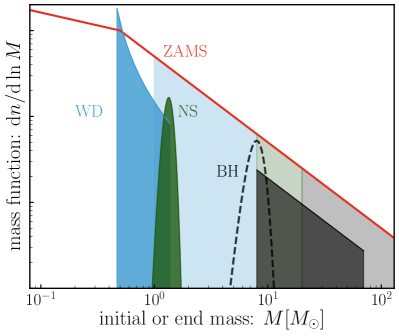
Figure 1: Broken power-law, red curve denotes the initial mass function of main-sequence stars assuming the Kroupa-like model (see Eq. 12). Note that $y$ axis is in an arbitrary scale. We assume that each massive star with $M_{\rm ZAMS}\geq 1~{}M_{\odot}$ has already evolved into its respective stellar remnant: white dwarfs (WD) for stars with $1\leq M_{\rm ZAMS}/M_{\odot}\leq 8$ following the initial and end mass relation, $M_{\rm WD}=0.339+0.129M_{\rm init}$ (blue line), neutron stars (NS) for $8\leq M_{\rm ZAMS}/M_{\odot}\leq 20$ (green), and stellar origin black holes (BH) for $M_{\rm ZAMS}\geq 20~{}M_{\odot}$, respectively. For BHs, we consider two models of the mass function; the black dashed line shows a Gaussian model with mean $M_{\rm final}=7.8M_{\odot}$ and width $\sigma=1.2M_{\odot}$, while the black solid line shows the power-law mass function with slope $\alpha_{\rm BH}=2$, i.e. the same slope as that for the ZAMS stars at the high mass end. For NS, we adopt the Gaussian model with $M_{\rm final}=1.33M_{\odot}$ and $\sigma=0.12M_{\odot}$ (green line). Because of the number conservation, the area under the curve for each stellar remnant, $\int\mathrm{d}\ln M~{}\mathrm{d}n/\mathrm{d}\ln M$, is the same as the area of the IMF over the corresponding range of initial main-sequence star masses (the two shaded regions of similar color have the same area).

We need to model mass functions (abundances) of lensing stars and stellar remnants to calculate the microlensing event rate. By stellar remnants we mean white dwarfs (WD), neutron stars (NS) and BHs, which are very faint or invisible, and therefore their genuine abundances are poorly understood. Throughout this paper we adopt the unified initial mass function of stars at birth, i.e. zero-age main-sequence stars (ZAMS), in both the Galactic bulge and disk regions. We then assume that, by today, massive stars of $M_{\rm ZAMS}\geq M_{\odot}$ have already evolved to form stellar remnants (WD, NS and BH). For visible objects, i.e. surviving main-sequence stars, we have a good idea of their spatial distribution in both the Galactic bulge and disk regions, which is hereafter referred to as the standard model of the Galactic structure. Our approach is to estimate the abundance of each stellar remnant population relative to that of main-sequence (MS) stars, assuming the number conservation between the ZAMS progenitors of the remnant population at birth and the remnants today. In our method, we include neither possible spatial inhomogeneities in the ZAMS mass function or stellar populations nor the star formation history, for simplicity. These simplified assumptions are appropriate here because we consider the abundances of stellar remnants relative to that of MS stars observed today. In addition, as long as the initial mass function of stars at birth has a similar form at each epoch of the star formation activities in the past (extending to sufficiently massive stars), the following results capture the main characteristics of the microlensing event rates. Nevertheless, these assumptions need to be revisited more carefully, and we should keep them in mind as a caveat of this approach.

We assume the following broken power-law mass function for ZAMS stars at birth: the number of stars in each logarithmic mass interval is given as

$$\frac{\mathrm{d}n_{\rm s}(M)}{\mathrm{d}\ln M}=\left\{\begin{array}[]{ll}{\displaystyle A_{\rm MS}\left(\frac{M}{0.5~{}M_{\odot}}\right)^{1-\alpha_{\rm MS1}}}\,,&(0.08\leq M/M_{\odot}\leq 0.5)\\ {\displaystyle A_{\rm MS}\left(\frac{M}{0.5~{}M_{\odot}}\right)^{1-\alpha_{\rm MS2}}}\,,&(M/M_{\odot}\geq 0.5),\end{array}\right.$$ (12)

where $A_{\rm MS}$ is the normalization constant that we will determine later; $A_{\rm MS}$ has a dimension of $[({\rm pc})^{-3}]$. In the following, we often omit the subscript “ZAMS” to denote mass of ZAMS star, $M_{\rm ZAMS}$, for notational simplicity. We adopt the Kroupa-like model for the mass function. Our default choices are $\alpha_{\rm MS1}=1.3$ and $\alpha_{\rm MS2}=2.0$ (Kroupa, 2001), because such a model nicely reproduces the timescale distribution of microlensing events in the OGLE observation as shown in Mroz et al. (2018) (also see Sumi et al., 2003, 2011; Niikura et al., 2019a). The number of ZAMS stars is dominated by low-mass stars.

Massive stars with $M\geq M_{\odot}$ have rapid evolution, and we assume that such massive stars have already evolved to stellar remnants. We assume ZAMS stars with $M_{\odot}\leq M_{\rm ZAMS}\leq 8M_{\odot}$ have evolved to WDs, ZAMS stars with $8M_{\odot}\leq M_{\rm ZAMS}\leq 20M_{\odot}$ to NSs, and ZAMS stars with $20M_{\odot}\leq M_{\rm ZAMS}\leq 100M_{\odot}$ to BHs. The critical assumption that we adopt throughout this paper is the number conservation between ZAMS stars and the stellar remnants. That is, we impose the number conservation:

$$\int_{M^{\rm ZAMS}_{{\rm SR},b}}^{M^{\rm ZAMS}_{{\rm SR},u}}\!\mathrm{d}\ln M\frac{\mathrm{d}n_{\rm s}}{\mathrm{d}\ln M}=\int_{0}^{\infty}\!\mathrm{d}\ln M_{\rm SR}~{}\phi(M_{\rm SR}),$$ (13)

where $\phi(M_{\rm SR})$ denotes the mass function of each stellar remnant (SR) population (WD, NS or BH) in the logarithmic mass interval, and $M^{\rm ZAMS}_{{\rm SR},b}$ and $M^{\rm ZAMS}_{{\rm SR},u}$ denote the lower- and upper-boundary masses, respectively, for the progenitor ZAMS stars of each stellar remnant; e.g., for WD, $M^{\rm ZAMS}_{{\rm WD},b}=M_{\odot}$ and $M^{\rm ZAMS}_{{\rm WD},u}=8M_{\odot}$. $M_{\rm SR}$ is the mass of the stellar remnant.

In the following, we describe the mass function for each population and how to determine the normalization.

• White dwarf (WD) – We assume that WDs form from ZAMS stars whose mass is not high enough to have a supernova explosion ($1\leq M_{\rm ZAMS}/M_{\odot}\leq 8$). After the red giant stage in the stellar evolutionary track, WDs are formed from the core of a star composed of carbon and oxygen. Here we adopt a simple mass conversion between the progenitor ZAMS mass and the final WD: $M_{\rm WD}=0.339+0.129M$ ($M_{\rm WD}$ and $M$ are in units of $M_{\odot}$) (Williams et al., 2009). Hence the mass function of WD is computed from

  $$\phi_{\rm WD}(M_{\rm WD})\mathrm{d}\ln M_{\rm WD}=\left.\frac{\mathrm{d}n_{\rm s}}{\mathrm{d}\ln M}\right|_{M=M(M_{\rm WD})}\mathrm{d}\ln M.$$ (14)

  The WD mass function is found to be

  $$\phi_{\rm WD}(M_{\rm WD}) =\left.\frac{\mathrm{d}n_{\rm s}}{\mathrm{d}\ln M}\right|_{M=M(M_{\rm WD})}\frac{\mathrm{d}\ln M}{\mathrm{d}\ln M_{\rm WD}}$$

  $$=A_{\rm MS}\left(\frac{M_{\rm WD}-0.339}{0.129\times 0.5M_{\odot}}\right)^{1-\alpha_{{\rm MS}2}}\frac{M_{\rm WD}}{M_{\rm WD}-0.339}.$$ (15)

• Neutron star (NS) – NSs originate from core-collapse supernovae of massive stars. Here we assume that massive ZAMS stars with $8\leq M_{\rm ZAMS}/M_{\odot}\leq 20$ evolve into NSs. We employ a simplified model; we assume that the mass function of NS follows a Gaussian distribution, so number conservation gives

  $$\int_{0}^{\infty}\mathrm{d}\ln M_{\rm NS}\phi_{\rm NS}(M_{\rm NS})=\int_{M=8}^{M=20}\mathrm{d}\ln M\frac{\mathrm{d}n_{\rm s}}{\mathrm{d}\ln M},$$ (16)

  with

  $$\phi_{\rm NS}(M_{\rm NS})\mathrm{d}\ln M_{\rm NS}\equiv\frac{A_{\rm NS}}{\sqrt{2\pi}\sigma_{\rm NS}}\exp\left[-\frac{(M_{\rm NS}-\bar{M}_{\rm NS})^{2}}{2\sigma_{\rm NS}^{2}}\right]\mathrm{d}M_{\rm NS},$$ (17)

  where $A_{\rm NS}$ is the normalization parameter (see below), and we adopt $\bar{M}_{\rm NS}=1.33M_{\odot}$ and $\sigma_{\rm NS}=0.12M_{\odot}$. Eq. (16) relates the normalization parameter $A_{\rm NS}$ to the normalization parameter of ZAMS, $A_{\rm MS}$, as

  $$A_{\rm NS}=\frac{A_{\rm MS}}{1-\alpha_{\rm MS2}}\left[\left(\frac{20}{0.5}\right)^{1-\alpha_{\rm MS2}}-\left(\frac{8}{0.5}\right)^{1-\alpha_{\rm MS2}}\right].$$ (18)

  Once the normalization of ZAMS mass function, $A_{\rm MS}$, is given, it determines the normalization of the NS mass function, $A_{\rm NS}$. Due to the Chandrasekhar limit (Shapiro & Teukolsky, 1983), NSs greater than a maximum mass limit ($\sim 2M_{\odot}$) do not exist (also see Özel & Freire, 2016, for a review).

• Black hole (BH) – BHs similarly originate from core collapse supernovae or perhaps direct collapse of very massive stars. However, the mass function of the resulting BHs is poorly known. Before the LIGO GW observations, it was thought that BH masses are in a narrow range around $\sim 8~{}M_{\odot}$ based on observations of $X$-ray binaries (Bailyn et al., 1998). However, the LIGO GW observations have revealed the existence of more massive BHs. The 10 GW events of BBH mergers, found by the OI/OII runs of the LIGO/VIRGO collaboration, indicate that a mass function of the BH progenitors is consistent with a Salpeter form, given as $\mathrm{d}n/\mathrm{d}M_{\rm BH}\propto M_{\rm BH}^{-2.3}$, although the constraint on the power-law slope is not tight (Abbott et al., 2019a). In this paper, we study how microlensing observation can be used to explore the shape of the BH mass function, and will consider several models of the BH mass function. Once the shape of BH mass function is assumed, we determine the normalization via the identity:

  $$\int_{0}^{\infty}\mathrm{d}\ln M_{\rm BH}~{}\phi_{\rm BH}(M_{\rm BH})=\int_{M=20}^{M=100}\mathrm{d}\ln M\frac{\mathrm{d}n_{\rm s}}{\mathrm{d}\ln M}.$$ (19)

  Throughout this paper we employ $100M_{\odot}$ for a maximum mass scale of ZAMS progenitors of BHs. This is not an important assumption, because the integration on the r.h.s. of the above equation is dominated by the lower bound, $20M_{\odot}$. Even if we change the upper bound to $70M_{\odot}$ from $100M_{\odot}$, it changes the abundance of BHs only by 10%.

The number conservations relating ZAMS stars to the surviving main-sequence stars and the stellar remnants give the following ratios of the numbers between different populations for our fiducial model of ZAMS initial mass function ($\alpha_{\rm MS1}=1.3$ and $\alpha_{\rm MS2}=2.0$ in Eq. 12):

$$\mbox{MS:WD:NS:BH}=1:0.13:0.011:0.0058.$$ (20)

Since our MW Galaxy consists of about $10^{11}$ stars, the ratio above means that there should be about 0.6 billion BHs in the MW in total, including both isolated systems and binary systems. As we described above, once the normalization parameter of ZAMS mass function, $A_{\rm MS}$, is given, we can obtain the normalizations of the mass functions for WD, NS, and BH. This is a critical procedure for the results in this paper.

The purpose of this paper is to discuss how a microlensing observation can be used to constrain the BH mass function. Hence we here employ a simple model for the BH mass function that is given by a handful of parameters. We consider the following power-law mass function as our default model:

$$\phi_{\rm BH}(M)\propto M^{1-\alpha_{\rm BH}}\hskip 10.00002pt\mbox{for}~{}M_{\rm min}\leq M\leq M_{\rm cut},$$ (21)

where $\alpha_{\rm BH}$ is a parameter to model the power-law index, $M_{\rm min}$ is a parameter to model the minimum BH mass, and $M_{\rm cut}$ is a parameter to model the maximum BH mass or the cut-off BH mass. Note that the power-law index is $1-\alpha_{\rm BH}$ instead of simply $\alpha_{\rm BH}$ since we define the mass function, $\phi_{\rm BH}$, as the number density per logarithmic interval of mass ($\mathrm{d}n/\mathrm{d}\ln M$). Our default model is given by $\alpha_{\rm BH}=2.0$, $M_{\rm min}=8~{}M_{\odot}$, and $M_{\rm cut}=70~{}M_{\odot}$. This model leads to $\bar{M}\simeq 19.6M_{\odot}$ for the average mass and $M_{0.45}\simeq 13.3M_{\odot}$ corresponding to the mass point where the normalized fraction of BHs is in the $45^{\text{th}}$ percentile. The latter number might be compared to Table 4 in Woosley et al. (2020). The number fraction of BHs above a certain mass is $f=0.77,0.32,0.17,0.097,0.05$ or 0.02 for BHs with masses greater than $10,20,30,40,50$ or $60M_{\odot}$, respectively. Combining this with Eq. (20), our default model assumes about $5.6\times 10^{-4}(\simeq 0.0058\times 0.097)$ BHs of $M\geq 40M_{\odot}$ per main-sequence star.

Fig. 1 illustrates how the mass function of ZAMS stars is related to mass functions of the stellar remnants, WD, NS and BH. As we described, ZAMS stars with $M_{\rm ZAMS}>1~{}M_{\odot}$ in the MW disk and bulge regions have already evolved into their respective stellar remnants. Since we impose the number conservation between the number of the progenitor ZAMS stars and that of the stellar remnants, the areas of the correspondingly colored shaded regions are the same. For BH, the black dashed line denotes the mass function that was thought reasonable before the LIGO GW observation; BHs have a narrow Gaussian distribution of their masses around $7.8~{}M_{\odot}$. The black solid line shows a Salpeter-like mass function, which is consistent with the 10 BBH GW events of the LIGO/Virgo observation (Abbott et al., 2019a); here we assume $\alpha_{\rm BH}=2.0$, $M_{\rm min}=8~{}M_{\odot}$ and $M_{\rm cut}=70~{}M_{\odot}$ for the parameters in Eq. (21). The areas under the dashed and solid black lines are the same, but these two models lead to totally different distributions of the microlensing timescales thanks to its strong dependence of the event rate on mass ($\mathrm{d}\Gamma/\mathrm{d}t_{E}\propto M^{2}$), as we will show below. Note that we assume there is a mass gap between NS and BH, in the range of $\sim[2,5]~{}M_{\odot}$, although there is a recent claim finding a BH in this mass range (Wyrzykowski & Mandel, 2020).

Furthermore, we assume a binary fraction of 0.4. For simplicity, we consider equal-mass binary systems: we treat microlensing of binary systems as a lens with mass $M_{\rm binary}=2M$ for each population. We do not consider binary systems that contain two objects of different masses or contain two objects of different populations (e.g., MS-WD system) for simplicity. Consequently we decrease the number of lens systems from the above numbers in Fig. 1 by the binary fraction. So we do not include the lensing effects of caustics in a binary lens (e.g. see Wyrzykowski et al., 2020, for the lightcurve due to a binary lens), and simply treat the effect by the increase in mass (i.e. by a point mass lens with doubled mass). Including the binary systems gives a slightly improved agreement between the model predictions and the OGLE data (Mróz et al., 2017; Niikura et al., 2019a).

3.2 A determination of the normalization of BH mass function

To further proceed with a calculation of the microlensing event rates (Eq. 6), we need to model the spatial and velocity distributions of the lensing objects (MS stars and the stellar remnants) in the Galactic bulge and disk regions. In this paper we employ the same method as in Niikura et al. (2019b), and here briefly describe the method.

For the mass distribution of the Galactic bulge, we employ the model of spheroidal mass profile as in Kent (1992):

$$\rho_{\rm b}(x,y,z)=\begin{cases}1.04~{}M_{\odot}/{\rm pc}^{3}\times{\displaystyle 10^{6}\left(\frac{s}{0.482}\right)^{-1.85}},&(s<938~{}{\rm pc})\\ 3.53~{}M_{\odot}/{\rm pc}^{3}~{}{\displaystyle K_{0}\!\left(\frac{s}{667}\right)},&(s\geq 938~{}{\rm pc}),\\ \end{cases}$$ (22)

where $K_{0}(x)$ is the modified Bessel function of zeroth order of the second kind, $s^{4}\equiv R^{4}$ + $(z/0.61)^{4}$, and $R^{2}\equiv x^{2}+y^{2}$ (see Section 2.2 for the definition of the coordinate system). Note the coordinates, $s$, $x$, $y$ and $z$ are all in units of parsec (pc).

For the Galactic disk, we employ the exponential disk model as in Bahcall (1986):

$$\rho_{\rm d}(R,z) =0.06~{}M_{\odot}/{\rm pc}^{3}\times\exp\left[-\left(\frac{R-8000}{3500}+\frac{|z|}{325}\right)\right].$$ (23)

This model assumes that the disk has an exponential mass distribution with vertical and radial scale lengths of 325 pc and 3500 pc, respectively.

The above Galactic bulge and disk models are based on various observations such as the luminosity functions and kinematics of stars. The Galactic bulge and disk models (Eqs. 22 and 23) have the form given by

$$\rho(x,y,z) =\rho_{\ast}f(x,y,z),$$ (24)

where $\rho_{\ast}$ is the normalization constant, which has a dimension of $[M_{\odot}/{\rm pc}^{3}]$, and the function $f(x,y,z)$ is a dimension-less function that describes the spatial structure of the mass distribution. For the models of Eqs. (22) and (23), $\rho_{\ast}=1.04$ or $3.53~{}M_{\odot}/{\rm pc}^{3}$ for the Galactic bulge, while $\rho_{\ast}=0.06~{}M_{\odot}/{\rm pc}^{3}$ for the Galactic disk.

Recalling the fact that the total stellar mass is given by the integral $\int\!\mathrm{d}\ln M~{}M\mathrm{d}n/\mathrm{d}\ln M$, the integrand peaks at $0.5~{}M_{\odot}$ as indicated by Fig. 1. This means that the stellar mass of the MW is dominated by MS stars around $\sim 0.5~{}M_{\odot}$. Assuming Eq. (12) for the mass function of MS stars, we can relate the normalization of the mass function, $A_{\rm MS}$, to the above $\rho_{\ast}$ via

$$\rho_{\ast}=\int_{0.08M_{\odot}}^{M_{\odot}}\!\!\mathrm{d}\ln M~{}M\frac{\mathrm{d}n}{\mathrm{d}\ln M}.$$ (25)

Inserting Eq. (12) with $\alpha_{\rm MS1}=1.3$ and $\alpha_{\rm MS2}=2.0$ into the above equation determines the normalization constant $A_{\rm MS}$:

$$A_{\rm MS}\simeq\frac{\rho_{\ast}}{0.863M_{\odot}}.$$ (26)

The dimension of $A_{\rm MS}$ is $[{\rm pc}^{-3}]$ (i.e. the dimension of the number density as desired). In turn, this determines the normalizations of WD, NS, and BH for an assumed form of the BH mass function. We further assume the same mass distribution for each of the MS stars and the stellar remnants (WD, NS, and BH) everywhere in the disk and bulge regions. For example, from Eqs. (17), (18) and (26), the spatial distribution of NS is given as

$$n_{\rm NS}(x,y,z;M_{\rm NS})\mathrm{d}M_{\rm NS} \simeq\frac{0.035\rho_{\ast}}{0.863M_{\odot}}f(x,y,z)$$

$$\times\frac{1}{\sqrt{2\pi}\sigma_{\rm NS}}\exp\left[-\frac{(M_{\rm NS}-\bar{M}_{\rm MS})^{2}}{2\sigma_{\rm NS}^{2}}\right]\mathrm{d}M_{\rm NS},$$ (27)

where we have used $A_{\rm NS}\simeq 0.035A_{\rm MS}$ from Eq. (18) assuming $\alpha_{\rm MS2}=2.0$. Similarly, we can determine the spatial distributions and mass spectra at each spatial position in the MW for MS stars, WD, and BH populations under the assumptions we employ.

3.3 The velocity distribution of BH

Now we describe the model of the velocity distribution for MS stars and the stellar remnants. We again employ the standard Galactic model for the velocity structure and assume that all the lensing objects obey the same velocity structure as that of MS stars, which are well studied by proper motion measurements (e.g. Qiu et al., 2020). BHs might have a kick velocity similar to that of neutron stars, which is believed to originate from asymmetric supernova explosions. However, in this paper we are most interested in massive BHs with $\geq 10~{}M_{\odot}$. Such massive BHs might be from a direct collapse (Belczynski et al., 2016) or a lifetime with less mass loss than that of lower mass BHs, such that they are sufficiently massive even after a supernova explosion (Vink et al., 2001). Hence, for such massive BHs, we would expect a small kick velocity. In this paper we simply assume the same velocity distribution for BHs as that of MS stars, and will give some discussion on this issue in the conclusion section.

The two-dimensional relative velocity components ${\bf v}_{\perp}$ (Eq. 7), relevant for microlensing, arise from combined contributions of the Galactic rotation and the random proper motions for each of source star, lens, and observer. We assume that the velocity function of ${\bf v}_{\perp}$ is given by the multiplicative form, for simplicity:

$$f({\bf v}_{\perp})\mathrm{d}^{2}{\bf v}_{\perp}=f(v_{y})f(v_{z})\mathrm{d}v_{y}\mathrm{d}v_{z}.$$ (28)

In this paper, we assume a Gaussian form for each velocity component, parameterized by the mean and the width:

$$f(v_{i})=\frac{1}{\sqrt{2\pi}\sigma_{v}}\exp\left[-\frac{(v_{i}-\bar{v})^{2}}{2\sigma_{v}^{2}}\right],$$ (29)

where $\bar{v}$ is the mean and $\sigma_{v}$ is the rms.

Following Han & Gould (1995), we assume that the velocity function for a lens in the bulge is given by

$$f_{y}:\left\{-220(1-\beta),\sqrt{1+\beta^{2}}100\right\}$$

$$f_{z}:\left\{0,\sqrt{1+\beta^{2}}100\right\},$$ (30)

where $\beta=d_{\rm l}/d_{\rm s}$, the first quantity in the curly brackets denotes the mean ($\bar{v}$), and the second quantity denotes the rms ($\sigma_{v}$). Note that all the quantities are in units of $[{\rm km}~{}{\rm s}^{-1}]$. Here we assume $100~{}{\rm km}~{}{\rm s}^{-1}$ for the random velocity dispersion per component and $220~{}{\rm km}~{}{\rm s}^{-1}$ for the Galactic rotation (rotation velocity of an observer with respect to the Galactic center). Here we also simply assume that the $y$-direction is along the Galactic rotation direction, which is a good approximation for an observation of the Galactic bulge region as $\ell,b\approx 0~{}$degrees.

For a lens in the Galactic disk, we assume that the velocity function is given by

$$f_{y}:\left\{220\beta,\sqrt{(\kappa\delta+30)^{2}+(100\beta)^{2}}\right\},$$

$$f_{z}:\left\{0,\sqrt{(\lambda\delta+30)^{2}+(100\beta)^{2}}\right\},$$ (31)

where $\kappa=5.625\times 10^{-3}~{}{\rm km}~{}{\rm s}^{-1}~{}{\rm pc}^{-1}$, $\lambda=3.75\times 10^{-3}~{}{\rm km}~{}{\rm s}^{-1}~{}{\rm pc}^{-1}$, and $\delta=x-8000~{}{\rm pc}$ ($x$ is in units of pc). Thus we include the spatial gradient of the velocity dispersion of stars against distance from the Galactic center.

4 Results

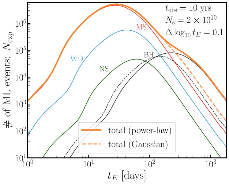
Figure 2: Expected number of microlensing events in each bin of the light curve timescale ($t_{E}$), for a hypothetical monitoring observation of source stars in the Galactic bulge region with the LSST, obtained by assuming the star and stellar remnant populations and the standard model of Galactic structures (spatial and velocity distributions). Here we assume $t_{\rm obs}=10~{}{\rm yrs}$ for the duration of observation, $N_{s}=2\times 10^{10}$ for the number of source stars, and $\Delta\log_{10}t_{E}=0.1$ (10 bins in one decade of $t_{E}$) corresponding to $\Delta\ln t_{E}\simeq 0.23$. We assume 60% efficiency for all the timescale microlensing events (see text for details), but note that the number events for low $t_{E}$ would be overestimated (an actual efficiency would be lower depending on details of the cadence). The thin red, blue and green lines are the contributions from main-sequence (MS) stars, white dwarfs (WD), and neutron stars (NS), respectively, assuming their mass functions in Fig. 1. The black dashed and solid lines are the contributions from black holes (BH) assuming the Gaussian and power-law mass functions in Fig. 1, respectively. The top, thick solid and dashed lines are the total contributions for the two models of black holes.

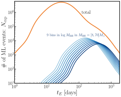
Figure 3: Similar to the previous plot, but blue lines show differential contributions of black holes, divided into different mass bins, to the total number of microlensing events. The top, thick line is the same as in Fig. 2, showing the total number obtained assuming the power-law mass function of black holes in Fig. 1. The blue lines show the contributions for each of 9 black hole subsamples that are evenly spaced in the logarithmic space of black hole mass in the range $M_{\rm BH}=[8,70]~{}M_{\odot}$. From light to dark lines, the central mass of each bin corresponds to $M_{\rm BH}/M_{\odot}\simeq 9$, 11, 15, 19, 24, 30, 38, 49, and $62$, respectively.

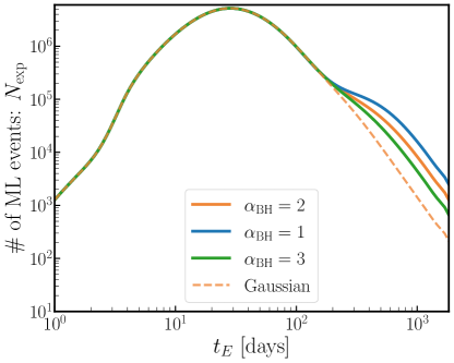
Figure 4: Dependence of the microlensing events on the mass slope of BH mass function. The orange solid and dashed lines are the same as those in Fig 2. The solid line is our default model, where we assume a Salpeter-like slope of $\alpha_{\rm BH}=2$ for the mass slope of BH mass function, defined as $\mathrm{d}n_{\rm BH}/\mathrm{d}\ln M\propto M^{1-\alpha_{\rm BH}}$. The blue and green lines are the results for $\alpha_{\rm BH}=1$ and 3, respectively. We impose the number conservation between ZAMS massive stars and BHs; the number of BHs in the Galactic bulge and disk regions are the same for all the models. For comparison, the thick, dashed line, the same as in Fig. 2, shows the model prediction for a model of Gaussian BH mass function in Fig. 1.

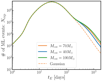
Figure 5: Similar to the previous figure, but dependence of the microlensing events on the maximum mass cut of BH in the Salpeter-like mass function ($\alpha_{\rm BH}=2$). While we assume $M_{\rm max}=70M_{\odot}$ for a maximum mass of BHs in our default model (orange line), the green and blue lines show the results if we assume $M_{\rm max}=40$ or 100$M_{\odot}$, respectively. Again we impose the number conservation: all the results have the same number of BHs.

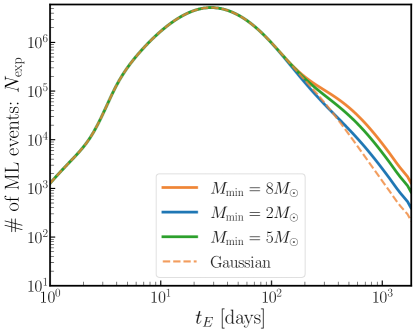
Figure 6: Similar to the previous figure, but in this figure we probe the microlensing dependence on BHs in the nominal mass gap ($[2,8]M_{\odot}$) by varying the minimum mass of BHs. In our fiducial model, we assume $M_{\rm min}=8M_{\odot}$ for a minimum mass of BHs (orange line). The green and blue lines are if we assume $M_{\rm min}=2$ or 5$M_{\odot}$, respectively. Again, all the results have the same number of BHs.

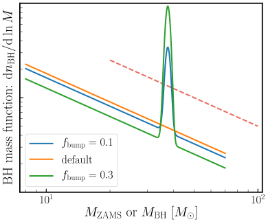
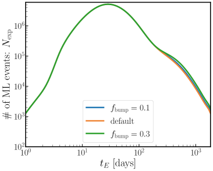
Figure 7: Upper panel: The BH mass function that is modeled by a sum of the power-law contribution and the Gaussian component, which is motivated by the recent study in Woosley et al. (2020). For the Gaussian component, we consider a Gaussian with mean $M_{\rm bump}=37.5M_{\odot}$ and width $\sigma=1M_{\odot}$, while we consider $\alpha_{\rm BH}=2$ for the slope of the power-law component. We parametrize the mass function by a fraction of the Gaussian component to the total number of BH: we consider $f_{\rm bump}=0$ (default), $0.1$, or $0.3$. All the models have the same number of BHs. For comparison, the dashed line shows the mass function of ZAMS progenitors of BHs. Lower panel: Expected number of microlensing events for the three cases of BH mass function.

We are now in a position to compute the event rate for each population (MS, WD, NS, or BH) by plugging the number density and velocity distributions of each population we have obtained up to the preceding section into Eq. (6). In this section, we show the main results of this paper.

4.1 The impact of LIGO-GW mass scale BHs on the microlensing events

The expected number of microlensing events in a given range of the $i$-th light curve timescale bin, $t_{E}=[t_{E,i}-\Delta t_{E,i}/2,t_{E,i}+\Delta t_{E,i}/2]$, for a given monitoring observation of the Galactic bulge region is given as

$$N_{\rm exp} =t_{\rm obs}N_{\rm s}\int_{t_{E,i}-\Delta\!t_{E,i}/2}^{t_{E,i}+\Delta\!t_{E,i}/2}\!\mathrm{d}t_{E}~{}\frac{\mathrm{d}\Gamma}{\mathrm{d}t_{E}}\epsilon(t_{E})$$

$$\simeq t_{\rm obs}N_{\rm s}\left.\frac{\mathrm{d}\Gamma}{\mathrm{d}t_{E}}\right|_{t_{E,i}}t_{E,i}\times\Delta\ln t_{E}\times\epsilon(t_{E,i}),$$ (32)

where $t_{\rm obs}$ is the duration of the monitoring observation, $N_{\rm s}$ is the number of source stars, $\Delta\ln t_{E}$ is the bin width in the logarithmic timescale intervals, and $\epsilon(t_{E})$ is a detection efficiency quantifying the probability that a microlensing event of timescale $t_{E}$ is detected by a given observation. In the following we consider logarithmically evenly-spaced bins of $t_{E}$, so $\Delta\ln t_{E}={\rm constant}$.

In this paper, we consider a hypothetical monitoring observation with LSST over 10 years (i.e. $t_{\rm obs}=10~{}$yrs). Thanks to the anticipated excellent image quality, the large aperture, and the wide field-of-view, LSST is expected to produce an ideal dataset for exploring microlensing events. Following Ivezić et al. (2019) we assume that such a dedicated LSST observation allows for monitoring observation of more than billions of stars in the Galactic bulge region: that is, we assume $N_{\rm s}=2\times 10^{10}$. This number is contrasted with that for the OGLE experiment, which has been using about $4.88\times 10^{7}$ source stars with the 1.3 m dedicated telescope (Mróz et al., 2017). Hence we think $N_{\rm s}=2\times 10^{10}$ for LSST is reasonable, but needs a more careful study based on actual data, e.g. data from the Dark Energy Camera as a pilot observation. As is obvious from the above equation, if we use a smaller number of source stars than what we assume, the number of events simply decreases by the ratio factor. A blending of multiple stars in the source plane will also have an effect on how many events we are able to observe (Niikura et al., 2019a). In the presence of blending effects, the observed amplification is modified by $A_{\rm obs}=(A-1)f_{s}+1$ where $A$ is the true amplification and $f_{s}$ is the normalized source flux such that $f_{s}$ = 1 in the absence of blending. As discussed in Wyrzykowski et al. (2015), the maximum efficiency with blending in OGLE-III is 60%. We would need a dedicated study to determine the efficiency function of LSST; e.g. we could use simulated images or inject simulated images of microlensing light curves into actual data, and then study the probability of recovering the injected events as a function of various observation conditions. This is beyond the scope of this paper. Instead, we will below discuss how efficiency depends on the observation cadence. As discussed in section 4.2, in particular, we expect the efficiency to be lower for the events with shorter Einstein crossing times. For the moment, we will assume $\epsilon$ = 0.6 since the effects of blending are thought to be similar to OGLE-III and therefore have a similar efficiency.

In Fig. 2 we show the expected number of microlensing events as a function of the light curve timescale $t_{E}$, expected for a hypothetical 10-year monitoring observation of $2\times 10^{10}$ stars in the Galactic bulge with LSST. Here we used the model described in Section 2. First of all, the figure clearly exhibits that LSST would enable one to find millions of microlensing events in each of timescale bins, showing the power of LSST, if $2\times 10^{10}$ source stars are used for the microlensing search. The different lines show the results for different populations of MS, WD, NS, and BH, assuming their mass functions in Fig. 1. Most notably, the black dashed and solid lines for the Gaussian and power-law mass function of BHs, respectively, give substantially different numbers of microlensing events, even though the two models have the same number of BHs. A power-law model for BHs predicts that BHs are a dominant source of microlensing events in each bin of $t_{E}\gtrsim 100~{}$days, even if the number of BHs is only 0.6% of the number of MS stars in our model (Eq. 20). To be more precise, an LSST observation would allow us to find about $6.1\times 10^{5}$ BH events. A Gaussian BH model leads to a factor of about 3 fewer events for microlensing events with $t_{E}>200~{}{\rm days}$, where the BH microlensing is a dominant source of the total events. For events at $t_{E}\gtrsim 10^{3}$ days, most events are from BHs with masses greater than $20M_{\odot}$. This boosted number of microlensing events at such long timescales is due to the mass boost in the microlensing event rate for such long-timescale events ($\Gamma\propto M^{2}$), as explained around Eq. (9). Also note that all lines of each population show an asymptotic behavior of $N_{\rm exp}\propto t_{E}^{-3}$ in large $t_{E}$ bins in this logarithmically-spaced binning, again as explained by Eq. (9). This is a consequence of the $t_{E}$-distributions if all the lens populations follow the same (or similar) spatial and velocity distributions. Thus we conclude that, if BHs have an underlying power-law mass distribution extending to $\gtrsim 20M_{\odot}$, a measurement of microlensing $t_{E}$-distribution allows for a direct test of the existence of such heavy BHs in the MW Galaxy, in the statistical sense. Since these events have a long timescale light curve, it would also be easier to make a follow-up observation of individual events, which would help to discriminate secure candidates of BH microlensing on an individual basis. Note that the numerical integration of Eq. (6) fully converges for $t_{E}\gtrsim 10^{2}$ days, which is our timescale of interest.

Blue lines in Fig. 3 show the differential contributions of BHs, divided into different mass bins, to the total event number. All the lines have an asymptotic behavior of the $t_{E}$-distribution as $N_{\rm exp}\propto t_{E}^{-3}$. The figure clearly shows that the microlensing events at longer timescales are dominated by heavier BHs, as expected. However, each line displays a wide $t_{E}$-distribution, spanning two orders of magnitude in $t_{E}$ ($x$-axis), with the range of event number varying over one order of magnitude ($y$-axis). BHs with $M\gtrsim 30M_{\odot}$ give about $2\times 10^{5}$ events, about one third of all BH events.

In Fig. 4 we study how varying the slope of the BH mass function, parametrized by $\mathrm{d}n_{\rm BH}/\mathrm{d}\ln M_{\rm BH}\propto M_{\rm BH}^{1-\alpha_{\rm BH}}$, alters the predictions of microlensing events. Our default model is a Salpeter-like mass function, given by $\alpha_{\rm BH}=2$. Note that all the models satisfy the number conservation between ZAMS massive stars and the BH remnants according to our method (Section 3): that is, all the models have the same number of BHs. As is obvious from the figure, increasing the relative populations of heavier BHs leads to a boost in the number of microlensing events at longer timescales. Among the three cases, the model with the shallowest slope, $\alpha_{\rm BH}=1$, leads to the largest population of such long-timescale events.

In Fig. 5 we study the model predictions for differing choices of the maximum mass cut in the BH mass function: $M_{\rm cut}=40$, 70, or $100M_{\odot}$, respectively, where $M_{\rm cut}=70M_{\odot}$ is our default model. Similarly to other figures, in this figure, the existence of heavier BHs leads to a larger number of events at longer timescales.

In light of the recent observation by LIGO of an object in the mass gap between black holes and neutron stars (Abbott et al., 2020a, b) and claims outside of gravitational wave detections (Thompson et al., 2019; Wyrzykowski & Mandel, 2020), we vary the lower limit of the LIGO black-hole mass function. In Fig. 6 we vary the lower limit of the BH mass function: $M_{\text{min}}$ = 2, 5, and 8 $M_{\odot}$ where $M_{\rm min}=8M_{\odot}$ is our default model. Again, heavier BHs leads to more events at longer timescales. Hence the existence of lower mass BHs, as in the case of $M_{\rm min}=2M_{\odot}$, leads to fewer events of longer timescales, because of the lowered normalization of the mass function for heavier BHs.

Moreover, motivated by the recent work (Woosley et al., 2020) that claims that BH mass might have a preferred mass scale at birth as a consequence of the stellar evolution, we also consider a contribution to microlensing arising from the secondary population of BHs, modeled by a Gaussian form with $M_{\rm bump}=37.5M_{\odot}$ and width $\sigma=1~{}M_{\odot}$. The preferred mass scale roughly corresponds to the mass scale of binary BH systems for the first LIGO GW event, GW150914 (Abbott et al., 2016b). In the upper panel of Fig. 7, we show the BH mass function which we model as a sum of the power-law and Gaussian contributions. We parametrize this model by a fraction of the Gaussian component, $f_{\rm bump}$, to the total number of BHs: here we consider $f_{\rm bump}=0.1$ or 0.3. The case of $f_{\rm bump}=0.1$ is intended to roughly reproduce Fig. 6 in (Woosley et al., 2020). Note that Fig. 6 in their paper plots $\mathrm{d}n_{\rm BH}/\mathrm{d}M$, instead of $\mathrm{d}n_{\rm BH}/\mathrm{d}\ln M$. This is a toy model, but the purpose is to study the impact of a specific feature in the BH mass function on the microlensing event rate. The lower panel of Fig. 7 shows the expected number of microlensing events. Even if the BH mass function has such a sharp feature around the particular mass scale, it does not imprint a corresponding feature in the $t_{E}$-distribution of microlensing events, as explained by Fig. 3. Therefore, we conclude that it is difficult to explore a narrow feature of the underlying BH mass function from the $t_{E}$-distribution of microlensing events in the statistical sense. Nevertheless, if we can make a follow-up study of individual secure events of BH microlensing, e.g. microlensing parallax and astrometric signal (Gould, 2000), it would be possible to reconstruct the mass distribution of BHs.

4.2 Evaluating LSST Cadences

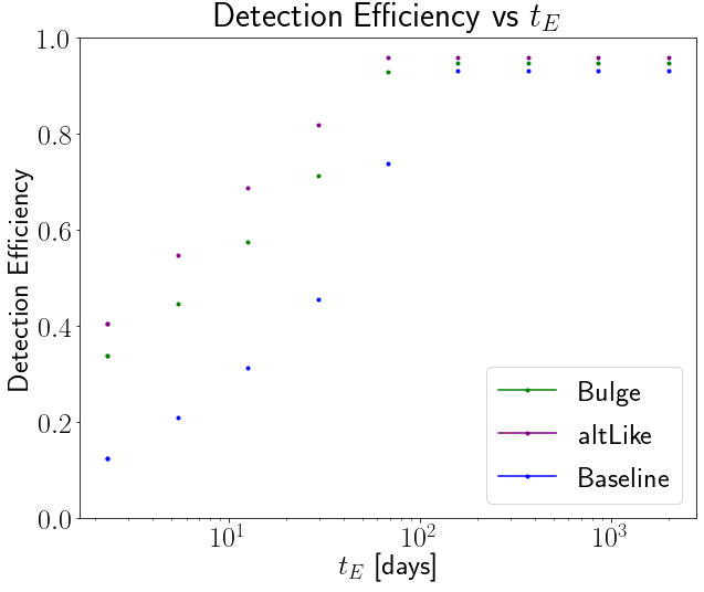
Figure 8: Detection efficiency of the three LSST cadences as a function of $t_{E}$ [days]. At low $t_{E}$, the altLike cadence does better than the bulge cadence which does better than the baseline cadence. However, at high $t_{E}$, all three are at approximately the same detection efficiency. They are not at 100% due to edge effects.

Here we study how a monitoring observation of the Galactic bulge with LSST allows us to explore microlensing events. To do this, we evaluate the performance of the three cadences considered in the LSST collaboration: the “baseline” cadence, which is an algorithmically determined cadence with a few deep drilling spots; the “bulge” focused cadence, which is a similarly algorithmically determined cadence with a focus on the Galactic bulge; and the “altLike” cadence, which is a deterministic cadence that scans the meridian of the sky as it passes overhead. The simulated cadences are from the OpSim database (Delgado & Reuter, 2016; Reuter et al., 2016) made by the Rubin Observatory team, which take into account historical weather conditions and other variables. We extract cadence information from eight fields around the bulge (270${}^{\circ},-30^{\circ}$) each ranging 3.5^∘ in RA and Dec around the center of the field of view to correspond to the LSST field of view. The center of each field of view is 4^∘ apart so they do not overlap.

To evaluate the cadences, we simulate 10,800 light curves with various $t_{E}$, $t_{0}$, and $u_{\rm min}$. We choose ten values of $t_{E}$ logarithmically spaced between 0 and 2000 days; the upper bound is due to the event rate dropping off at around this value (see Fig. 2). We choose 120 values of $t_{0}$ spaced evenly for the 10 year survey, so there is one month between each value. We choose ten values of $u_{\rm min}$, evenly spaced from 0 to 1. We then sample these light curves with the simulated cadences.

We consider a microlensing event “detected” with A $\geq$ 1.1 and at least four observations on either side of the peak of the simulated light curve. This ensures that it is observed at least two nights before and after the magnification peak since often two observations will be taken on one night.

By plotting the detection efficiency (see Fig. 8) as a function of $t_{E}$, we can see that the “altLike” cadence achieves the highest efficiency, the bulge cadence achieves the second highest, and the baseline cadence achieves the lowest. At high Einstein crossing times (over 100 days), there is no significant difference between the cadences. At maximum efficiency they detect nearly all the events. It is likely that the cadences do not detect all of the events due to some of the events having their peak extremely close to when the cadences begin or end their observations, so the telescope is unable to make four observations before and after the peak for those events. Note that this evaluation does not include the presence of parallax, which is a useful quantity for identifying black holes (see section 5).

5 Discussion and Conclusion

In this paper we have studied how microlensing observation can be used to explore a population of BHs that exist in the Galactic bulge and disk regions, motived by the LIGO/Virgo GW events due to binary black hole systems that indicate a population of heavier BHs with masses $\gtrsim 30~{}M_{\odot}$ than the previously anticipated mass scale of $\sim 8M_{\odot}$. We showed that, if BHs have a Salpeter-like mass function extending up to $70M_{\odot}$ in our default model, the BH population yields a dominant source of microlensing events at longer timescales, $t_{E}\gtrsim 100~{}{\rm days}$ (Fig. 2). We showed that a tiny population of such heavier BHs could alter the $t_{E}$-distribution of microlensing events at such long timescales due to the boost of microlensing event rates given by $M^{2}$ for a fixed $t_{E}$ (Figs. 3–5). In our fiducial model, we assume about $6\times 10^{-4}$ BHs of $\geq 40M_{\odot}$ per main-sequence star. To find this result we assume the number conservation between BHs and the massive progenitors of zero-age main sequence stars and that the BH population follows the same spatial and velocity structures as those of the surviving main sequence stars in the Galactic bulge and disk regions. If LSST carries out a suitable cadence observation to monitor $2\times 10^{10}$ source stars towards the Galactic bulge over 10 years, it could detect about $6\times 10^{5}$ BH microlensing events thanks to its unique capability. However, the Galactic bulge region usually has a large dust extinction, so it requires a more careful study of how an optical telescope such as LSST can carry out an efficient microlensing observation in the bulge region. Our results might be compared to Lam et al. (2020), which shows different event rates from our results. The difference is mainly from the different BH mass function; Lam et al. (2020) employed the BH mass function with maximum mass cut around $M\sim 16M_{\odot}$, and did not include a population of the heavier BHs in the event rate evaluation.

The origin of LIGO/Virgo BHs is poorly understood. As we showed, microlensing can be a powerful tool to explore the nature of the BH population in the MW. Here, microlensing is complementary to the statistical method using the GW BBH events, which are sensitive to close-orbit and heavier BHs due to the dependences of LIGO/Virgo GW sensitivities on properties of BBH systems. On the other hand, microlensing is sensitive to both isolated BHs and wide-orbit BBH systems. If a characteristic signature in the microlensing light curve due to binary systems is detected, the microlensing method could provide useful information on the binary fraction of BHs. Furthermore combining the microlensing constraints and the LIGO BBH population studies would give a coherent picture of the origin of the BH population.

A major assumption in our analysis is that the velocity distribution of BHs is the same as that of the main sequence stars, which has been well studied. BHs may have a large kick velocity due to anisotropic supernova explosions, so they may have faster velocities on average than main sequence stars do. A faster-moving, heavier lens would produce a similar microlensing timescale to that of a slower-moving, lighter lens. Thus an observation of the light curve alone would cause degeneracies in parameters of individual lenses. In addition, if BHs have faster velocities on average than those of main-sequence stars, it would weaken the shoulder-like feature of the $t_{E}$-distribution in Fig. 2 (the $t_{E}$-distribution of BHs would shift left horizontally in the figure). To overcome this obstacle, a detailed follow-up observation of individual secure candidates of BH microlensing would be useful. For example, we can explore the microlensing parallax and astrometric signal (Gould, 2000) (also see Gaudi et al., 2008; Bennett et al., 2010) to disentangle the parameter degeneracies. Such parallax signals have been measured successfully (Poindexter et al., 2005; Wyrzykowski et al., 2016), though the parallax is not enough to completely break the degeneracy. Through astrometric microlensing, one can solve for the Einstein radius and therefore the mass of the lens (Dominik & Sahu, 2000; Rybicki et al., 2018; Lu et al., 2016). Measuring the parallax would be possible via LSST itself through the year-timescale monitoring observation due to the orbital motion of the Earth and/or if the Roman Space Telescope jointly monitored the light curve of the same object at the same time; the upcoming Gaia NIR mission might also be a helpful monitor (Hobbs et al., 2019). Combining the light curve with proper motion measurements, pre- or post-microlensing observation would also be useful. For a BH lens system, one can only observe the source star, so one could disentangle properties of the lens-source system provided the combined information of proper motion and source flux (Wyrzykowski & Mandel, 2020), if the source star is resolved. The Japan-led JASMINE satellite project (Kobayashi et al., 2012) would give useful information on the proper motion, if the observation region has an overlap with the LSST microlensing observation region. The European Extremely Large Telescope would also be useful thanks to the superb angular resolution by adaptive optics. These are all interesting possibilities worth further investigation to be presented elsewhere.

References

- Abbott et al. (2016a) Abbott, B. P., Abbott, R., Abbott, T. D., et al. 2016a, Physical Review Letters, 116, 061102, doi: 10.1103/PhysRevLett.116.061102
- Abbott et al. (2016b) —. 2016b, Phys. Rev. Lett., 116, 061102, doi: 10.1103/PhysRevLett.116.061102
- Abbott et al. (2017) —. 2017, ApJ, 851, L35, doi: 10.3847/2041-8213/aa9f0c
- Abbott et al. (2019a) —. 2019a, ApJ, 882, L24, doi: 10.3847/2041-8213/ab3800
- Abbott et al. (2019b) —. 2019b, Physical Review X, 9, 031040, doi: 10.1103/PhysRevX.9.031040
- Abbott et al. (2020a) —. 2020a, ApJ, 892, L3, doi: 10.3847/2041-8213/ab75f5
- Abbott et al. (2020b) Abbott, R., Abbott, T. D., Abraham, S., et al. 2020b, ApJ, 896, L44, doi: 10.3847/2041-8213/ab960f
- Alcock et al. (2000) Alcock, C., Allsman, R. A., Alves, D. R., et al. 2000, ApJ, 542, 281, doi: 10.1086/309512
- Antonini & Perets (2012) Antonini, F., & Perets, H. B. 2012, ApJ, 757, 27, doi: 10.1088/0004-637X/757/1/27
- Bahcall (1986) Bahcall, J. N. 1986, ARA&A, 24, 577, doi: 10.1146/annurev.aa.24.090186.003045
- Bailyn et al. (1998) Bailyn, C. D., Jain, R. K., Coppi, P., & Orosz, J. A. 1998, ApJ, 499, 367, doi: 10.1086/305614
- Beaulieu et al. (2006) Beaulieu, J. P., Bennett, D. P., Fouqué, P., et al. 2006, Nature, 439, 437, doi: 10.1038/nature04441
- Belczynski et al. (2016) Belczynski, K., Holz, D. E., Bulik, T., & O’Shaughnessy, R. 2016, Nature, 534, 512, doi: 10.1038/nature18322
- Belczynski et al. (2002) Belczynski, K., Kalogera, V., & Bulik, T. 2002, ApJ, 572, 407, doi: 10.1086/340304
- Bennett et al. (2002) Bennett, D. P., Becker, A. C., Quinn, J. L., et al. 2002, ApJ, 579, 639, doi: 10.1086/342225
- Bennett et al. (2010) Bennett, D. P., Rhie, S. H., Nikolaev, S., et al. 2010, ApJ, 713, 837, doi: 10.1088/0004-637X/713/2/837
- Bethe & Brown (1998) Bethe, H. A., & Brown, G. E. 1998, ApJ, 506, 780, doi: 10.1086/306265
- Binney & Tremaine (2008) Binney, J., & Tremaine, S. 2008, Galactic Dynamics: Second Edition
- Bird et al. (2016) Bird, S., Cholis, I., Muñoz, J. B., et al. 2016, Physical Review Letters, 116, 201301, doi: 10.1103/PhysRevLett.116.201301
- Bond et al. (2010) Bond, N. A., Ivezić, Ž., Sesar, B., et al. 2010, ApJ, 716, 1, doi: 10.1088/0004-637X/716/1/1
- Carr et al. (2020) Carr, B., Kohri, K., Sendouda, Y., & Yokoyama, J. 2020, arXiv e-prints, arXiv:2002.12778. https://arxiv.org/abs/2002.12778
- Delgado & Reuter (2016) Delgado, F., & Reuter, M. A. 2016, in Society of Photo-Optical Instrumentation Engineers (SPIE) Conference Series, Vol. 9910, Proc. SPIE, 991013, doi: 10.1117/12.2233630
- Dominik & Sahu (2000) Dominik, M., & Sahu, K. C. 2000, ApJ, 534, 213, doi: 10.1086/308716
- Drlica-Wagner et al. (2019) Drlica-Wagner, A., Mao, Y.-Y., Adhikari, S., et al. 2019, arXiv e-prints, arXiv:1902.01055. https://arxiv.org/abs/1902.01055
- Gaia Collaboration et al. (2018) Gaia Collaboration, Brown, A. G. A., Vallenari, A., et al. 2018, A&A, 616, A1, doi: 10.1051/0004-6361/201833051
- Gaudi et al. (2008) Gaudi, B. S., Bennett, D. P., Udalski, A., et al. 2008, Science, 319, 927, doi: 10.1126/science.1151947
- Godines et al. (2020) Godines, D., Bachelet, E., Narayan, G., & Street, R. A. 2020, arXiv e-prints, arXiv:2004.14347. https://arxiv.org/abs/2004.14347
- Gould (2000) Gould, A. 2000, ApJ, 542, 785, doi: 10.1086/317037
- Griest et al. (1991) Griest, K., Alcock, C., Axelrod, T. S., et al. 1991, ApJ, 372, L79, doi: 10.1086/186028
- Han & Gould (1995) Han, C., & Gould, A. 1995, ApJ, 447, 53, doi: 10.1086/175856
- Han & Gould (1996) —. 1996, ApJ, 467, 540, doi: 10.1086/177631
- Helmi (2020) Helmi, A. 2020, arXiv e-prints, arXiv:2002.04340. https://arxiv.org/abs/2002.04340
- Hobbs et al. (2019) Hobbs, D., Brown, A., Høg, E., et al. 2019, arXiv e-prints, arXiv:1907.12535. https://arxiv.org/abs/1907.12535
- Ivezic et al. (2008) Ivezic, Z., Tyson, J. A., Abel, B., et al. 2008, ArXiv e-prints:0805.2366. https://arxiv.org/abs/0805.2366
- Ivezić et al. (2019) Ivezić, Ž., Kahn, S. M., Tyson, J. A., et al. 2019, ApJ, 873, 111, doi: 10.3847/1538-4357/ab042c
- Kent (1992) Kent, S. M. 1992, ApJ, 387, 181, doi: 10.1086/171070
- Kobayashi et al. (2012) Kobayashi, Y., Shimura, Y., Niwa, Y., et al. 2012, in Society of Photo-Optical Instrumentation Engineers (SPIE) Conference Series, Vol. 8442, Proc. SPIE, 844247, doi: 10.1117/12.924870
- Kroupa (2001) Kroupa, P. 2001, MNRAS, 322, 231, doi: 10.1046/j.1365-8711.2001.04022.x
- Kusenko et al. (2020) Kusenko, A., Sasaki, M., Sugiyama, S., et al. 2020, arXiv e-prints, arXiv:2001.09160. https://arxiv.org/abs/2001.09160
- Lam et al. (2020) Lam, C. Y., Lu, J. R., Hosek, Matthew W., J., Dawson, W. A., & Golovich, N. R. 2020, ApJ, 889, 31, doi: 10.3847/1538-4357/ab5fd3
- Lu et al. (2019) Lu, J. R., Lam, C. Y., Medford, M., Dawson, W., & Golovich, N. 2019, Research Notes of the American Astronomical Society, 3, 58, doi: 10.3847/2515-5172/ab1421
- Lu et al. (2016) Lu, J. R., Sinukoff, E., Ofek, E. O., Udalski, A., & Kozlowski, S. 2016, ApJ, 830, 41, doi: 10.3847/0004-637X/830/1/41
- Mao & Paczynski (1991) Mao, S., & Paczynski, B. 1991, ApJ, 374, L37, doi: 10.1086/186066
- Mao & Paczynski (1996) —. 1996, ApJ, 473, 57, doi: 10.1086/178126
- Mao et al. (2002) Mao, S., Smith, M. C., Woźniak, P., et al. 2002, MNRAS, 329, 349, doi: 10.1046/j.1365-8711.2002.04986.x
- McKernan et al. (2012) McKernan, B., Ford, K. E. S., Lyra, W., & Perets, H. B. 2012, MNRAS, 425, 460, doi: 10.1111/j.1365-2966.2012.21486.x
- Mróz et al. (2017) Mróz, P., Udalski, A., Skowron, J., et al. 2017, Nature, 548, 183, doi: 10.1038/nature23276
- Mroz et al. (2018) Mroz, P., Udalski, A., Bennett, D. P., et al. 2018, arXiv e-prints. https://arxiv.org/abs/1811.00441
- Mróz et al. (2020) Mróz, P., Udalski, A., Szymański, M. K., et al. 2020, ApJS, 249, 16, doi: 10.3847/1538-4365/ab9366
- Niikura et al. (2019a) Niikura, H., Takada, M., Yokoyama, S., Sumi, T., & Masaki, S. 2019a, Phys. Rev. D, 99, 083503, doi: 10.1103/PhysRevD.99.083503
- Niikura et al. (2019b) Niikura, H., Takada, M., Yasuda, N., et al. 2019b, Nature Astronomy, 3, 524, doi: 10.1038/s41550-019-0723-1
- Özel & Freire (2016) Özel, F., & Freire, P. 2016, ARA&A, 54, 401, doi: 10.1146/annurev-astro-081915-023322
- Paczynski (1986) Paczynski, B. 1986, ApJ, 304, 1, doi: 10.1086/164140
- Poindexter et al. (2005) Poindexter, S., Afonso, C., Bennett, D. P., et al. 2005, ApJ, 633, 914, doi: 10.1086/468182
- Portegies Zwart & McMillan (2000) Portegies Zwart, S. F., & McMillan, S. L. W. 2000, ApJ, 528, L17, doi: 10.1086/312422
- Qiu et al. (2020) Qiu, T., Wang, W., Takada, M., et al. 2020, arXiv e-prints, arXiv:2004.12899. https://arxiv.org/abs/2004.12899
- Reuter et al. (2016) Reuter, M. A., Cook, K. H., Delgado, F., Petry, C. E., & Ridgway, S. T. 2016, in Society of Photo-Optical Instrumentation Engineers (SPIE) Conference Series, Vol. 9911, Proc. SPIE, 991125, doi: 10.1117/12.2232680
- Rybicki et al. (2018) Rybicki, K. A., Wyrzykowski, Ł., Klencki, J., et al. 2018, MNRAS, 476, 2013, doi: 10.1093/mnras/sty356
- Sasaki et al. (2016) Sasaki, M., Suyama, T., Tanaka, T., & Yokoyama, S. 2016, Physical Review Letters, 117, 061101, doi: 10.1103/PhysRevLett.117.061101
- Shapiro & Teukolsky (1983) Shapiro, S. L., & Teukolsky, S. A. 1983, Black holes, white dwarfs, and neutron stars : the physics of compact objects
- Sugiyama et al. (2020) Sugiyama, S., Kurita, T., & Takada, M. 2020, MNRAS, 493, 3632, doi: 10.1093/mnras/staa407
- Sumi et al. (2003) Sumi, T., Abe, F., Bond, I. A., et al. 2003, ApJ, 591, 204, doi: 10.1086/375212
- Sumi et al. (2011) Sumi, T., Kamiya, K., Bennett, D. P., et al. 2011, Nature, 473, 349, doi: 10.1038/nature10092
- Thompson et al. (2019) Thompson, T. A., Kochanek, C. S., Stanek, K. Z., et al. 2019, Science, 366, 637, doi: 10.1126/science.aau4005
- Tisserand et al. (2007) Tisserand, P., Le Guillou, L., Afonso, C., et al. 2007, A&A, 469, 387, doi: 10.1051/0004-6361:20066017
- Udalski et al. (1994) Udalski, A., Szymanski, M., Kaluzny, J., et al. 1994, ApJ, 426, 69, doi: 10.1086/187342
- Vink et al. (2001) Vink, J. S., de Koter, A., & Lamers, H. J. G. L. M. 2001, A&A, 369, 574, doi: 10.1051/0004-6361:20010127
- Williams et al. (2009) Williams, K. A., Bolte, M., & Koester, D. 2009, ApJ, 693, 355, doi: 10.1088/0004-637X/693/1/355
- Wood & Mao (2005) Wood, A., & Mao, S. 2005, MNRAS, 362, 945, doi: 10.1111/j.1365-2966.2005.09357.x
- Woosley et al. (2020) Woosley, S., Sukhbold, T., & Janka, H. T. 2020, arXiv e-prints, arXiv:2001.10492. https://arxiv.org/abs/2001.10492
- Wyrzykowski & Mandel (2020) Wyrzykowski, L., & Mandel, I. 2020, A&A, 636, A20, doi: 10.1051/0004-6361/201935842
- Wyrzykowski et al. (2015) Wyrzykowski, Ł., Rynkiewicz, A. E., Skowron, J., et al. 2015, ApJS, 216, 12, doi: 10.1088/0067-0049/216/1/12
- Wyrzykowski et al. (2016) Wyrzykowski, Ł., Kostrzewa-Rutkowska, Z., Skowron, J., et al. 2016, MNRAS, 458, 3012, doi: 10.1093/mnras/stw426
- Wyrzykowski et al. (2020) Wyrzykowski, Ł., Mróz, P., Rybicki, K. A., et al. 2020, A&A, 633, A98, doi: 10.1051/0004-6361/201935097
- Yang et al. (2019) Yang, Y., Bartos, I., Gayathri, V., et al. 2019, Phys. Rev. Lett., 123, 181101, doi: 10.1103/PhysRevLett.123.181101