On the Conditional Expectation of Mean Shifted Gaussian Distributions

Abstract

In this paper, we consider a property of univariate Gaussian distributions namely conditional expectation shift (or centroid shift). Specifically, we compare two Gaussian distributions in which they differ only in their means. Equivalently, we can view this situation as one of the distribution is shifted to the right. These two distributions are conditioned on the same event in which the realizations fall in the right interval or left interval. We show that if a Gaussian distribution is shifted to the right while the conditioning event remains the same then the conditional expectation is shifted to the right concurrently.

1 Problem

Define the centroid of a function $f:\mathbb{R}\to\mathbb{R}$ under a support $\mathcal{S}\subseteq\mathbb{R}$ as

$$\langle f\rangle_{\mathcal{S}}\triangleq\frac{1}{\int_{\mathcal{S}}f(x)dx}\cdot\int_{\mathcal{S}}xf(x)dx=\frac{1}{\int f(x)\cdot\mathbbm{1}_{\mathcal{S}}(x)dx}\cdot\int xf(x)\cdot\mathbbm{1}_{\mathcal{S}}(x)dx.$$ (1)

where the indicator function $\mathbbm{1}_{\mathcal{S}}:\mathbb{R}\to\{0,1\}$ is defined as

$$\mathbbm{1}_{\mathcal{S}}(x)=\begin{cases}1\quad\text{if}\;\;x\in\mathcal{S},\\ 0\quad\text{if}\;\;x\notin\mathcal{S}.\end{cases}$$

However, if we consider $f_{\boldsymbol{X}}$ which is the probability density function (pdf) of a random variable $\boldsymbol{X}$, the above definition coincides with the conditional expectation given that $\boldsymbol{X}\in\mathcal{S}$ as shown below:

$$\mathbb{E}[\boldsymbol{X}|\boldsymbol{X}\in\mathcal{S}] =\int xf_{\boldsymbol{X}}(x|\boldsymbol{X}\in\mathcal{S})dx$$

$$=\frac{1}{P(\boldsymbol{X}\in\mathcal{S})}\cdot\int_{\mathcal{S}}xf(x)dx$$

$$=\frac{1}{\int_{\mathcal{S}}f_{\boldsymbol{X}}(x)dx}\cdot\int_{\mathcal{S}}xf_{\boldsymbol{X}}(x)dx$$

$$=\langle f_{\boldsymbol{X}}\rangle_{\mathcal{S}}.$$

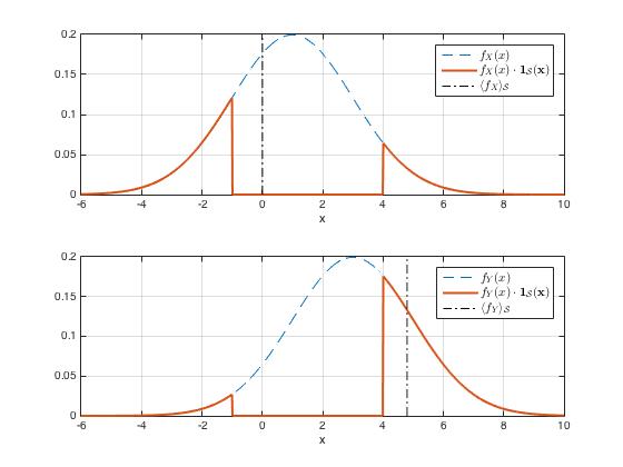
In particular, we consider two univariate Gaussian random variables $\boldsymbol{X}$ and $\boldsymbol{Y}$ in which their pdfs differ only in their means namely $\mathcal{N}(\mu,\sigma^{2})$ and $\mathcal{N}(\mu+h,\sigma^{2})$, respectively, i.e., the variance of distributions is the same. We are interested in the relationship between conditional expectation of these two random variables. Specifically, given that $\boldsymbol{X}\in\mathcal{S}$ and $\boldsymbol{Y}\in\mathcal{S}$ where $\mathcal{S}=(-\infty,\ell]\cup[u,\infty)$ for some constant $u>\ell$, does it hold true that the conditional expectation of $\boldsymbol{Y}$ is strictly greater than that of $\boldsymbol{X}$ when $h>0$? In other words, we want to show that when $h>0$, $\langle f_{\boldsymbol{Y}}\rangle_{\mathcal{S}}>\langle f_{\boldsymbol{X}}\rangle_{\mathcal{S}}$ where $f_{\mathchoice{\mathbin{\vbox{\hbox{\scalebox{0.5}{$\displaystyle\bullet$}}}}}{\mathbin{\vbox{\hbox{\scalebox{0.5}{$\textstyle\bullet$}}}}}{\mathbin{\vbox{\hbox{\scalebox{0.5}{$\scriptstyle\bullet$}}}}}{\mathbin{\vbox{\hbox{\scalebox{0.5}{$\scriptscriptstyle\bullet$}}}}}}$ is the pdf of the random variable “$\boldsymbol{\mathchoice{\mathbin{\vbox{\hbox{\scalebox{0.5}{$\displaystyle\bullet$}}}}}{\mathbin{\vbox{\hbox{\scalebox{0.5}{$\textstyle\bullet$}}}}}{\mathbin{\vbox{\hbox{\scalebox{0.5}{$\scriptstyle\bullet$}}}}}{\mathbin{\vbox{\hbox{\scalebox{0.5}{$\scriptscriptstyle\bullet$}}}}}}$”. Hence the name “conditional expectation shift” or “controid shift”. To clarify the concept, we provide an example illustrated in Figure 1. In the next section, we provide the theorem regrading to this question and also its proof.

Figure 1: In this example, we use $\mu=1$, $\sigma^{2}=4$, and $h=2$, i.e., $\boldsymbol{X}\sim\mathcal{N}(1,4)$ and $\boldsymbol{Y}\sim\mathcal{N}(3,4)$. Also, we set $\ell=-1$ and $u=4$ which means that $\mathcal{S}=(-\infty,-1]\cup[4,\infty)$. We also calculate the centroid of both functions; $f_{\boldsymbol{X}}(x)\cdot\mathbbm{1}_{\mathcal{S}}(x)$ and $f_{\boldsymbol{Y}}(x)\cdot\mathbbm{1}_{\mathcal{S}}(x)$. The centroids are $\langle f_{\boldsymbol{X}}\rangle_{\mathcal{S}}\approx 0.0025$ and $\langle f_{\boldsymbol{Y}}\rangle_{\mathcal{S}}\approx 4.7995$. In this case, we can see that $\langle f_{\boldsymbol{Y}}\rangle_{\mathcal{S}}>\langle f_{\boldsymbol{X}}\rangle_{\mathcal{S}}$.

2 Main Theorem and Proof

Theorem 1.

Suppose

$$f(x)=\frac{1}{\sqrt{2\pi\sigma^{2}}}\exp{\Big{(}-\frac{1}{2\sigma^{2}}(x-\mu)^{2}\Big{)}}$$ (2)

with $\mu\in\mathbb{R}$ and $\sigma\in\mathbb{R}_{>0}$. Let $g(x)=f(x-h)$ and $\mathcal{S}=\mathbb{R}\setminus(\ell,u)$. Then, for all $h\in\mathbb{R}_{>0}$, and $\ell,u\in\mathbb{R}$ such that $u>\ell$,

$$\langle g\rangle_{\mathcal{S}}>\langle f\rangle_{\mathcal{S}}.$$ (3)

Proof.

First, we will show that it is necessary and sufficient to consider

$$\langle\hat{g}\rangle_{\hat{\mathcal{S}}}>\langle\hat{f}\rangle_{\hat{\mathcal{S}}}$$

instead of the inequality (3), where

$$\hat{f}(x)=\frac{1}{\sqrt{2\pi}}\exp{\Big{(}-\frac{1}{2}x^{2}\Big{)}},$$

i.e., the pdf of a random variable $\hat{\boldsymbol{X}}\sim\mathcal{N}(0,1)$, $\hat{g}(x)=\hat{f}(x-\hat{h})$ with $\hat{h}=\frac{h}{\sigma}$, and $\hat{\mathcal{S}}=\mathbb{R}\setminus(\hat{\ell},\hat{u})$ with $\hat{u}=\frac{u-\mu}{\sigma}$ and $\hat{\ell}=\frac{\ell-\mu}{\sigma}$.

Consider the term $\int_{\mathcal{{S}}}xg(x)dx$ as follows:

$$\int_{\mathcal{{S}}}xg(x)dx=\int_{\mathcal{S}}\frac{x}{\sqrt{2\pi\sigma^{2}}}\exp{\Big{(}-\frac{1}{2\sigma^{2}}(x-h-\mu)^{2}\Big{)}}dx.$$

By substituting $x=\sigma t+\mu$, we get

$$\int_{\mathcal{{S}}}xg(x)dx =\int_{\hat{\mathcal{S}}}(\sigma t+\mu)\cdot\frac{1}{\sqrt{2\pi}}\exp{\Big{(}-\frac{1}{2}\Big{(}t-\frac{h}{\sigma}\Big{)}^{2}\Big{)}}dt$$

$$=\sigma\int_{\hat{\mathcal{S}}}\frac{t}{\sqrt{2\pi}}\exp{\Big{(}-\frac{1}{2}(t-\hat{h})^{2}\Big{)}}dt+\mu\int_{\hat{\mathcal{S}}}\frac{1}{\sqrt{2\pi}}\exp{\Big{(}-\frac{1}{2}(t-\hat{h})^{2}\Big{)}}dt$$

$$=\sigma\int_{\hat{\mathcal{S}}}t\hat{g}(t)dt+\mu\int_{\hat{\mathcal{S}}}\hat{g}(t)dt.$$

Then, consider the term $\int_{\mathcal{{S}}}g(x)dx$ as follows:

$$\int_{\mathcal{{S}}}g(x)dx=\int_{\mathcal{S}}\frac{1}{\sqrt{2\pi\sigma^{2}}}\exp{\Big{(}-\frac{1}{2\sigma^{2}}(x-h-\mu)^{2}\Big{)}}dx.$$

Again, by substituting $x=\sigma t+\mu$, we get

$$\int_{\mathcal{{S}}}g(x)dx=\int_{\hat{\mathcal{S}}}\frac{1}{\sqrt{2\pi}}\exp{\Big{(}-\frac{1}{2}\Big{(}t-\frac{h}{\sigma}\Big{)}^{2}\Big{)}}dt=\int_{\hat{\mathcal{S}}}\frac{1}{\sqrt{2\pi}}\exp{\Big{(}-\frac{1}{2}(t-\hat{h})^{2}\Big{)}}dt=\int_{\hat{\mathcal{S}}}\hat{g}(t)dt.$$

Therefore, using the definition of the centroid of a function (1), we obtain that

$$\langle g\rangle_{\mathcal{S}}=\frac{1}{\int_{\mathcal{S}}g(x)dx}\cdot\int_{\mathcal{S}}xg(x)dx=\mu+\frac{\sigma}{\int_{\hat{\mathcal{S}}}\hat{g}(x)dx}\cdot\int_{\hat{\mathcal{S}}}x\hat{g}(x)dx=\mu+\sigma\langle\hat{g}\rangle_{\hat{\mathcal{S}}}.$$ (4)

In fact, the above analysis holds for any $h\in\mathbb{R}$. By letting $h=0$, we also obtain that

$$\langle f\rangle_{\mathcal{S}}=\mu+\sigma\langle\hat{f}\rangle_{\hat{\mathcal{S}}}.$$ (5)

Since $\sigma\in\mathbb{R}_{>0}$, substituting the expressions (4) and (5) into (3) yields

$$\langle g\rangle_{\mathcal{S}}>\langle f\rangle_{\mathcal{S}}\quad\Longleftrightarrow\quad\langle\hat{g}\rangle_{\hat{\mathcal{S}}}>\langle\hat{f}\rangle_{\hat{\mathcal{S}}}$$

which proves the claim.

The claim suggests that without loss of generality, we can consider

$$f(x)=\frac{1}{\sqrt{2\pi}}\exp{\Big{(}-\frac{1}{2}x^{2}\Big{)}},$$ (6)

i.e., the standard Gaussian distribution, instead of the one in (2). To simplify the notation, starting from here we will stick to the expression of $f$ in (6). Before moving on to the next claim, consider

$$\int_{\mathcal{S}}xg(x)dx =\int_{\mathcal{S}}\frac{x}{\sqrt{2\pi}}\exp{\Big{(}-\frac{1}{2}(x-h)^{2}\Big{)}}dx$$

$$=h\int_{\mathcal{S}^{\prime}}\frac{1}{\sqrt{2\pi}}\exp{\Big{(}-\frac{1}{2}x^{2}\Big{)}}dx+\int_{\mathcal{S}^{\prime}}\frac{x}{\sqrt{2\pi}}\exp{\Big{(}-\frac{1}{2}x^{2}\Big{)}}dx$$

$$=h\int_{\mathcal{S}^{\prime}}f(x)dx+\int_{\mathcal{S}^{\prime}}\frac{x}{\sqrt{2\pi}}\exp{\Big{(}-\frac{1}{2}x^{2}\Big{)}}dx$$ (7)

where $\mathcal{S}^{\prime}=\mathbb{R}\setminus(\ell-h,u-h)$. And,

$$\int_{\mathcal{S}}g(x)dx=\int_{\mathcal{S}}\frac{1}{\sqrt{2\pi}}\exp{\Big{(}-\frac{1}{2}(x-h)^{2}\Big{)}}dx=\int_{\mathcal{S}^{\prime}}\frac{1}{\sqrt{2\pi}}\exp{\Big{(}-\frac{1}{2}x^{2}\Big{)}}dx=\int_{\mathcal{S}^{\prime}}f(x)dx.$$ (8)

However, we can simplify the last term on the RHS of (7) as follows:

$$\int_{\mathcal{S}^{\prime}}\frac{x}{\sqrt{2\pi}}\exp{\Big{(}-\frac{1}{2}x^{2}\Big{)}}dx =\int_{-\infty}^{\ell-h}\frac{x}{\sqrt{2\pi}}\exp{\Big{(}-\frac{1}{2}x^{2}\Big{)}}dx+\int_{u-h}^{\infty}\frac{x}{\sqrt{2\pi}}\exp{\Big{(}-\frac{1}{2}x^{2}\Big{)}}dx$$

$$=\frac{1}{\sqrt{2\pi}}\Big{[}-\exp{(-x)}\Big{]}_{x=\infty}^{x=\frac{1}{2}(\ell-h)^{2}}+\frac{1}{\sqrt{2\pi}}\Big{[}-\exp{(-x)}\Big{]}_{x=\frac{1}{2}(u-h)^{2}}^{x=\infty}$$

$$=\frac{1}{\sqrt{2\pi}}\exp{\Big{(}-\frac{1}{2}(u-h)^{2}\Big{)}}-\frac{1}{\sqrt{2\pi}}\exp{\Big{(}-\frac{1}{2}(\ell-h)^{2}\Big{)}}$$

$$=f(u-h)-f(\ell-h).$$ (9)

Using the equations (7), (8) and (9), we can write

$$\langle g\rangle_{\mathcal{S}} =\frac{1}{\int_{\mathcal{S}}g(x)dx}\cdot\int_{\mathcal{S}}xg(x)dx$$

$$=\frac{1}{\int_{\mathcal{S}^{\prime}}f(x)dx}\bigg{[}h\int_{\mathcal{S}^{\prime}}f(x)dx+\big{(}f(u-h)-f(\ell-h)\big{)}\bigg{]}$$

$$=h+\frac{f(u-h)-f(\ell-h)}{\int_{\mathcal{S}^{\prime}}f(x)dx}.$$ (10)

To simplify the term $\int_{\mathcal{S}^{\prime}}f(x)dx$ in (10), we define $\Phi:\mathbb{R}\to[0,1]$ to be the cumulative distribution function (cdf) of the standard Gaussian distribution $f$, i.e.,

$$\Phi(x)\triangleq\int_{-\infty}^{x}\frac{1}{\sqrt{2\pi}}\exp{\Big{(}-\frac{1}{2}t^{2}\Big{)}}dt=\int_{-\infty}^{x}f(t)dt$$

and define $\mathcal{Q}:\mathbb{R}\to[0,1]$ to be the tail distribution function of the standard Gaussian distribution $f$, i.e.,

$$\mathcal{Q}(x)\triangleq\int_{x}^{\infty}\frac{1}{\sqrt{2\pi}}\exp{\Big{(}-\frac{1}{2}t^{2}\Big{)}}dt=\int_{x}^{\infty}f(t)dt.$$

Note that $\Phi(x)+\mathcal{Q}(x)=1$ and $\mathcal{Q}(-x)=\Phi(x)$ for all $x\in\mathbb{R}$. With these definitions in hand, we can rewrite the term $\int_{\mathcal{S}^{\prime}}f(x)dx$ in (10) as

$$\int_{\mathcal{S}^{\prime}}f(x)dx=\int_{-\infty}^{\ell-h}f(x)dx+\int_{u-h}^{\infty}f(x)dx=\Phi(\ell-h)+\mathcal{Q}(u-h).$$

Therefore, the equation (10) becomes

$$\langle g\rangle_{\mathcal{S}}=h+\frac{f(u-h)-f(\ell-h)}{\mathcal{Q}(u-h)+\Phi(\ell-h)}.$$

Since $g(x)=f(x-h)$, we have

$$\langle f\rangle_{\mathcal{S}}=\langle g\rangle_{\mathcal{S}}\Big{|}_{h=0}=\frac{f(u)-f(\ell)}{\mathcal{Q}(u)+\Phi(\ell)}.$$

For fixed $u$, $\ell\in\mathbb{R}$ (with $u>\ell$), define a function $\Psi:\mathbb{R}\to\mathbb{R}$ to be

$$\Psi(h)\triangleq h+\frac{f(u-h)-f(\ell-h)}{\mathcal{Q}(u-h)+\Phi(\ell-h)}.$$ (11)

Notice that $\Psi(h)=\langle g\rangle_{\mathcal{S}}$ and $\Psi(0)=\langle f\rangle_{\mathcal{S}}$. Next, we want to show that for all $h\in\mathbb{R}$,

$$\frac{d}{dh}\Psi(h)>0.$$

The derivative can be expressed as

$$\frac{d}{dh}\Psi(h)=1+\frac{1}{\big{[}\mathcal{Q}(u-h)+\Phi(\ell-h)\big{]}^{2}}\cdot\Big{\{}\big{[}\mathcal{Q}(u-h)+\Phi(\ell-h)\big{]}\frac{d}{dh}\big{[}f(u-h)-f(\ell-h)\big{]}\\ -\big{[}f(u-h)-f(\ell-h)\big{]}\frac{d}{dh}\big{[}\mathcal{Q}(u-h)+\Phi(\ell-h)\big{]}\Big{\}}.$$ (12)

Suppose $c\in\mathbb{R}$ is a constant. We will simplify some expressions as follows.

$$\frac{d}{dh}f(c-h) =\frac{1}{\sqrt{2\pi}}\frac{d}{dh}\exp{\Big{(}-\frac{1}{2}(c-h)^{2}\Big{)}}$$

$$=(c-h)\cdot\frac{1}{\sqrt{2\pi}}\exp{\Big{(}-\frac{1}{2}(c-h)^{2}\Big{)}}$$

$$=(c-h)f(c-h).$$ (13)

Since $\Phi(x)$ is the cdf of the standard Gaussian distribution and $\mathcal{Q}(x)=1-\Phi(x)$ for any $x\in\mathbb{R}$, we have

$$\frac{d}{dh}\Phi(c-h)=-f(c-h)\quad\text{and}\quad\frac{d}{dh}\mathcal{Q}(c-h)=f(c-h).$$ (14)

Applying the expressions (13) and (14) to (12), we obtain that

$$\frac{d}{dh}\Psi(h) =1+\frac{\big{[}(u-h)f(u-h)-(\ell-h)f(\ell-h)\big{]}\big{[}\mathcal{Q}(u-h)+\Phi(\ell-h)\big{]}-\big{[}f(u-h)-f(\ell-h)\big{]}^{2}}{\big{[}\mathcal{Q}(u-h)+\Phi(\ell-h)\big{]}^{2}}$$

$$=\frac{1}{\big{[}\mathcal{Q}(u-h)+\Phi(\ell-h)\big{]}^{2}}\cdot\Big{\{}\big{[}(u-h)f(u-h)-(\ell-h)f(\ell-h)\big{]}\big{[}\mathcal{Q}(u-h)+\Phi(\ell-h)\big{]}$$

$$\qquad\qquad\qquad\qquad\qquad+\big{[}\mathcal{Q}(u-h)+\Phi(\ell-h)\big{]}^{2}-\big{[}f(u-h)-f(\ell-h)\big{]}^{2}\Big{\}}.$$

Since $\big{[}\mathcal{Q}(u-h)+\Phi(\ell-h)\big{]}^{2}>0$ for all $h\in\mathbb{R}$, we can consider only the term in the curly bracket. Define a function $\Omega:\mathbb{R}\times\mathbb{R}\to\mathbb{R}$ to be

$$\Omega(x_{1},x_{2})\triangleq\big{(}x_{1}f(x_{1})-x_{2}f(x_{2})\big{)}\big{(}\mathcal{Q}(x_{1})+\Phi(x_{2})\big{)}+\big{(}\mathcal{Q}(x_{1})+\Phi(x_{2})\big{)}^{2}-\big{(}f(x_{1})-f(x_{2})\big{)}^{2}.$$ (15)

If we can show that $\Omega(x_{1},x_{2})>0$ for all $x_{1},x_{2}\in\mathbb{R}$, this implies $\frac{d}{dh}\Psi(h)>0$ for all $h\in\mathbb{R}$ which is our desired result.

Before we proceed, let’s derive a lower bound of the ratios $\frac{\mathcal{Q}(x)}{2f(x)}$ and $\frac{\Phi(x)}{2f(x)}$. Consider the inequality [1, Formula 7.1.13]

$$\exp{(x^{2})}\int_{x}^{\infty}\exp{(-t^{2})}dt>\frac{1}{x+\sqrt{x^{2}+2}}$$ (16)

which holds for all $x\in\mathbb{R}$. Using the substitution $t=\frac{v}{\sqrt{2}}$, we have

$$\exp{(x^{2})}\int_{x}^{\infty}\exp{(-t^{2})}dt=\frac{1}{\sqrt{2}}\exp{(x^{2})}\int_{\sqrt{2}x}^{\infty}\exp{\Big{(}-\frac{1}{2}v^{2}\Big{)}}dv$$ (17)

Combining (16) and (17) together and using substitution $x=\frac{z}{\sqrt{2}}$ to obtain

$$\frac{1}{\sqrt{2}}\exp{\Big{(}\frac{1}{2}z^{2}\Big{)}}\int_{z}^{\infty}\exp{\Big{(}-\frac{1}{2}v^{2}\Big{)}}dv>\frac{1}{\frac{z}{\sqrt{2}}+\sqrt{\frac{z^{2}}{2}+2}}$$

which is equivalent to (by multiplying both sides by $\frac{1}{\sqrt{2}}$ and renaming the variables)

$$\frac{\mathcal{Q}(x)}{2f(x)}=\frac{\frac{1}{\sqrt{2\pi}}\int_{x}^{\infty}\exp{\big{(}-\frac{1}{2}t^{2}\big{)}}dt}{2\cdot\frac{1}{\sqrt{2\pi}}\exp{\big{(}-\frac{1}{2}x^{2}\big{)}}}>\frac{1}{x+\sqrt{x^{2}+4}}.$$ (18)

In order to get the lower bound of $\frac{\Phi(x)}{2f(x)}$, we substitute $x=-z$ into (18) to get

$$\frac{\mathcal{Q}(-z)}{2f(-z)}>\frac{1}{-z+\sqrt{z^{2}+4}}.$$

Using the properties $\mathcal{Q}(-z)=\Phi(z)$ and $f(-z)=f(z)$ for all $z\in\mathbb{R}$ (and renaming the variable) yields

$$\frac{\Phi(x)}{2f(x)}>\frac{1}{-x+\sqrt{x^{2}+4}}.$$ (19)

From the lower bound (18), for all $x_{1}\in\mathbb{R}$, we have

$$\frac{\mathcal{Q}(x_{1})}{2f(x_{1})}>\frac{1}{x_{1}+\sqrt{x_{1}^{2}+4}}=\frac{1}{4}\big{(}-x_{1}+\sqrt{x_{1}^{2}+4}\big{)}$$

$$\Longleftrightarrow\quad \big{(}2\mathcal{Q}(x_{1})+x_{1}f(x_{1})\big{)}-\sqrt{x_{1}^{2}+4}\cdot f(x_{1})>0.$$ (20)

On the other hand, from the lower bound (19), for all $x_{2}\in\mathbb{R}$, we have

$$\frac{\Phi(x_{2})}{2f(x_{2})}>\frac{1}{-x_{2}+\sqrt{x_{2}^{2}+4}}=\frac{1}{4}\big{(}x_{2}+\sqrt{x_{2}^{2}+4}\big{)}$$

$$\Longleftrightarrow\quad \big{(}2\Phi(x_{2})-x_{2}f(x_{2})\big{)}-\sqrt{x_{2}^{2}+4}\cdot f(x_{2})>0.$$ (21)

Summing the inequalities (20) and (21) together yields

$$2\big{[}\mathcal{Q}(x_{1})+\Phi(x_{2})\big{]}+\big{[}x_{1}f(x_{1})-x_{2}f(x_{2})\big{]}-\Big{[}\sqrt{x_{1}^{2}+4}\cdot f(x_{1})+\sqrt{x_{2}^{2}+4}\cdot f(x_{2})\Big{]}>0.$$ (22)

Since $x_{1}+\sqrt{x_{1}^{2}+4}>0$ for all $x_{1}\in\mathbb{R}$ and $-x_{2}+\sqrt{x_{2}^{2}+4}>0$ for all $x_{2}\in\mathbb{R}$, we have

$$\Big{(}x_{1}+\sqrt{x_{1}^{2}+4}\Big{)}f(x_{1})+\Big{(}-x_{2}+\sqrt{x_{2}^{2}+4}\Big{)}f(x_{2})>0$$

$$\Longrightarrow\quad 2\big{[}\mathcal{Q}(x_{1})+\Phi(x_{2})\big{]}+\Big{(}x_{1}+\sqrt{x_{1}^{2}+4}\Big{)}f(x_{1})+\Big{(}-x_{2}+\sqrt{x_{2}^{2}+4}\Big{)}f(x_{2})>0$$

$$\Longleftrightarrow\quad 2\big{[}\mathcal{Q}(x_{1})+\Phi(x_{2})\big{]}+\big{[}x_{1}f(x_{1})-x_{2}f(x_{2})\big{]}+\Big{[}\sqrt{x_{1}^{2}+4}\cdot f(x_{1})+\sqrt{x_{2}^{2}+4}\cdot f(x_{2})\Big{]}>0$$

Multiplying both sides of (22) by the term on the LHS of the inequality above yields

$$\Big{\{}2\big{[}\mathcal{Q}(x_{1})+\Phi(x_{2})\big{]}+\big{[}x_{1}f(x_{1})-x_{2}f(x_{2})\big{]}\Big{\}}^{2}-\Big{[}\sqrt{x_{1}^{2}+4}\cdot f(x_{1})+\sqrt{x_{2}^{2}+4}\cdot f(x_{2})\Big{]}^{2}>0.$$

Simplify the above inequality to get

$$\big{[}x_{1}f(x_{1})-x_{2}f(x_{2})\big{]}\big{[}\mathcal{Q}(x_{1})+\Phi(x_{2})\big{]}+\big{[}\mathcal{Q}(x_{1})+\Phi(x_{2})\big{]}^{2}\\ +\frac{1}{4}\Big{\{}\big{[}x_{1}f(x_{1})-x_{2}f(x_{2})\big{]}^{2}-\Big{[}\sqrt{x_{1}^{2}+4}\cdot f(x_{1})+\sqrt{x_{2}^{2}+4}\cdot f(x_{2})\Big{]}^{2}\Big{\}}>0.$$

Using the definition of $\Omega(x_{1},x_{2})$ in (15), we can rewrite the above inequality as

$$\Omega(x_{1},x_{2})+\big{[}f(x_{1})-f(x_{2})\big{]}^{2}\\ +\frac{1}{4}\Big{\{}\big{[}x_{1}f(x_{1})-x_{2}f(x_{2})\big{]}^{2}-\Big{[}\sqrt{x_{1}^{2}+4}\cdot f(x_{1})+\sqrt{x_{2}^{2}+4}\cdot f(x_{2})\Big{]}^{2}\Big{\}}>0.$$ (23)

We will show that

$$\big{[}f(x_{1})-f(x_{2})\big{]}^{2}+\frac{1}{4}\Big{\{}\big{[}x_{1}f(x_{1})-x_{2}f(x_{2})\big{]}^{2}-\Big{[}\sqrt{x_{1}^{2}+4}\cdot f(x_{1})+\sqrt{x_{2}^{2}+4}\cdot f(x_{2})\Big{]}^{2}\Big{\}}<0$$ (24)

which implies that $\Omega(x_{1},x_{2})>0$ from (23) as desired.

Consider the second term on the LHS of (24) as follows:

$$\frac{1}{4}\Big{\{}\big{[}x_{1}f(x_{1})-x_{2}f(x_{2})\big{]}^{2}-\Big{[}\sqrt{x_{1}^{2}+4}\cdot f(x_{1})+\sqrt{x_{2}^{2}+4}\cdot f(x_{2})\Big{]}^{2}\Big{\}}$$

$$=\; \frac{1}{4}\Big{\{}\big{[}x_{1}^{2}f^{2}(x_{1})+x_{2}^{2}f^{2}(x_{2})-2x_{1}x_{2}f(x_{1})f(x_{2})\big{]}$$

$$\qquad\qquad\qquad\qquad-\Big{[}(x_{1}^{2}+4)f^{2}(x_{1})+(x_{2}^{2}+4)f^{2}(x_{2})+2\sqrt{x_{1}^{2}+4}\sqrt{x_{2}^{2}+4}\cdot f(x_{1})f(x_{2})\Big{]}\Big{\}}$$

$$=\; -f^{2}(x_{1})-f^{2}(x_{2})-\frac{1}{2}x_{1}x_{2}f(x_{1})f(x_{2})-\frac{1}{2}\sqrt{x_{1}^{2}+4}\sqrt{x_{2}^{2}+4}\cdot f(x_{1})f(x_{2}).$$

Thus, the term on the LHS of (24) becomes

$$\big{[}f(x_{1})-f(x_{2})\big{]}^{2}+\frac{1}{4}\Big{\{}\big{[}x_{1}f(x_{1})-x_{2}f(x_{2})\big{]}^{2}-\Big{[}\sqrt{x_{1}^{2}+4}\cdot f(x_{1})+\sqrt{x_{2}^{2}+4}\cdot f(x_{2})\Big{]}^{2}\Big{\}}$$

$$=\; -2f(x_{1})f(x_{2})-\frac{1}{2}x_{1}x_{2}f(x_{1})f(x_{2})-\frac{1}{2}\sqrt{x_{1}^{2}+4}\sqrt{x_{2}^{2}+4}\cdot f(x_{1})f(x_{2})$$

$$=\; -\Big{[}2+\frac{1}{2}\Big{(}x_{1}x_{2}+\sqrt{x_{1}^{2}+4}\sqrt{x_{2}^{2}+4}\Big{)}\Big{]}f(x_{1})f(x_{2}).$$

Since $f(x_{1})f(x_{2})>0$ for all $x_{1},x_{2}\in\mathbb{R}$, it remains to show that

$$x_{1}x_{2}+\sqrt{x_{1}^{2}+4}\sqrt{x_{2}^{2}+4}>0$$

for all $x_{1},x_{2}\in\mathbb{R}$. Consider the positive expression for all $x_{1},x_{2}\in\mathbb{R}$ below:

$$4x_{1}^{2}+4x_{2}^{2}+16 >0$$

$$\Longleftrightarrow\quad x_{1}^{2}x_{2}^{2}+4x_{1}^{2}+4x_{2}^{2}+16 >x_{1}^{2}x_{2}^{2}$$

$$\Longleftrightarrow\quad(x_{1}^{2}+4)(x_{2}^{2}+4) >x_{1}^{2}x_{2}^{2}$$

$$\Longleftrightarrow\quad\sqrt{x_{1}^{2}+4}\sqrt{x_{2}^{2}+4} >|x_{1}x_{2}|$$

$$\Longrightarrow\quad\sqrt{x_{1}^{2}+4}\sqrt{x_{2}^{2}+4} >-x_{1}x_{2}$$

$$\Longleftrightarrow\quad\sqrt{x_{1}^{2}+4}\sqrt{x_{2}^{2}+4}+x_{1}x_{2} >0.$$

Again, this means that the inequality (24) holds for all $x_{1},x_{2}\in\mathbb{R}$. Thus, $\Omega(x_{1},x_{2})>0$ for all $x_{1},x_{2}\in\mathbb{R}$ as discussed earlier (where $\Omega(x_{1},x_{2})$ is defined in (15)). Consequently, we have proved the claim $\frac{d}{dh}\Psi(h)>0$ for all $h\in\mathbb{R}$ or equivalently, $\Psi(h)$ is a strictly increasing function. In particular, for $h\in\mathbb{R}_{>0}$, we have

$$\langle g\rangle_{\mathcal{S}}=\Psi(h)>\Psi(0)=\langle f\rangle_{\mathcal{S}}$$

from the definition of $\Psi(h)$ in (11), which completes the proof. ∎

References

• [1] M.ย Abramowitz and I.ย A. Stegun, Handbook of mathematical functions with formulas, graphs, and mathematical tables.ย ย ย US Government printing office, 1948, vol.ย 55.