Fast Subtrajectory Similarity Search in Road Networks under Weighted Edit Distance Constraints

Abstract

In this paper, we address a similarity search problem for spatial trajectories in road networks. In particular, we focus on the subtrajectory similarity search problem, which involves finding in a database the subtrajectories similar to a query trajectory. A key feature of our approach is that we do not focus on a specific similarity function; instead, we consider weighted edit distance (WED), a class of similarity functions which allows user-defined cost functions and hence includes several important similarity functions such as EDR and ERP. We model trajectories as strings, and propose a generic solution which is able to deal with any similarity function belonging to the class of WED. By employing the filter-and-verify strategy, we introduce subsequence filtering to efficiently prunes trajectories and find candidates. In order to choose a proper subsequence to optimize the candidate number, we model the choice as a discrete optimization problem (NP-hard) and compute it using a 2-approximation algorithm. To verify candidates, we design bidirectional tries, with which the verification starts from promising positions and leverage the shared segments of trajectories and the sparsity of road networks for speed-up. Experiments are conducted on large datasets to demonstrate the effectiveness of WED and the efficiency of our method for various similarity functions under WED.

1 Introduction

Vehicular transportation is facing a crucial turning point as data-driven information technology advances. Data-driven approaches, such as intelligent routing and ride-sharing, are expected to resolve important social issues, such as environmental problem and traffic congestion; they are therefore actively studied in many fields, including database research. Accordingly, fundamental operations, such as indexing and retrieval, on huge vehicular trajectory data are becoming increasingly important [48, 41, 64, 20, 22, 21, 19].

This paper addresses the similarity search problem over trajectories in road networks, which is a classical but still active area of spatial database research [48, 41, 64, 56, 55]. Unlike most existing studies that target whole matching between data and query trajectories (i.e., the entire trajectories are similar), we tackle the subtrajectory similarity search problem, which finds in a vehicular trajectory database the subtrajectories similar to a query (Figure 1).

Why subtrajectory similarity search?  One motivating application is travel time estimation along a given path. Recent on-the-fly approaches [52, 53] estimate the travel time distribution by retrieving historical trajectories that contain the query path as a subtrajectory immediately after the query arrived. Other applications include alternative route suggestion that finds the variations of a query path in the database as alternative routes and path popularity estimation [20, 28, 8] that counts the frequency of appearance of a given path in the database as a subtrajectory.

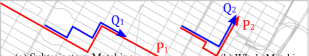
Figure 1: Subtrajectory matching/Whole matching.

Exact path queries have been studied for subtrajectory search [22, 20]; however, exact path queries only find trajectories containing a subtrajectory that exactly matches a query trajectory. Hence similarity queries are adopted to retrieve more semantically relevant results for various applications [63, 17, 6, 7, 58, 39, 48, 41, 64, 45]. For example, similarity queries can handle the errors caused by sampling strategies, spatial transformations, or natural noises [7, 6, 48, 64, 45], which are common in real data. In addition, travel time estimation suffers from data sparsity (i.e., there are few historical trajectories that exactly travel a query path in the specified time slot) even in urban areas. Subtrajectory similarity queries have been used to address this issue; e.g., by path similarity [16] or road segment similarity (types, number of lanes, etc.) [51], based on the observation that paths or road segments with similar contexts may have similar travel time.

Trajectory similarity functions.  To measure the similarity between trajectories, a similarity function must be selected. Albeit many trajectory similarity functions have been proposed [63, 42, 7, 6, 58, 39, 40, 48, 55, 64, 56, 11, 14, 46], as demonstrated experimentally [48, 64, 7, 6]), every similarity function has its own advantages and disadvantages. In other words, there is no “best” trajectory similarity function, and the choice depends on the application scenario. Accordingly, for trajectory similarity search, general methodologies that do not depend on a specific similarity function are preferable.

In this paper, we consider weighted edit distance (WED), a class of similarity functions that includes several ones commonly used in trajectory analysis, such as edit distance on real sequences (EDR) [7] and edit distance with real penalty (ERP) [6], which have been shown capable of handling different sampling strategies, spatial transformations, and/or noises, and better than other functions such as dynamic time warping (DTW) and longest common subsequence (LCSS) [45]. WED is flexible in the sense that it allows user-defined cost functions. As such, it not only covers EDR and ERP but also their extensions (e.g., the adaptations using road network distance instead of binary or Euclidean distance). WED also captures the semantics of the aforementioned similarities for travel time estimation [16, 51], and is able to measure the road segments that differ between two trajectories, thereby (reversely) expressing semantics similar to longest overlapping road segments (LORS) [48] and longest common road segments (LCRS) [64].

Challenges.  For real applications like trajectory analysis [41, 64], it is desirable to return query results in seconds or even less. Trajectories in road networks can be modeled as strings, and the problem is converted to substring search. A naive approach is scanning the database using the Smith-Waterman algorithm [43]; however, this is inefficient for large datasets as it does not employ indexing. For fast query processing, most string similarity algorithms resort to the filter-and-verify paradigm, which finds a set of candidates and then verify them. The most widely used is $q$-gram filtering [13, 57, 36, 10, 54] (also for trajectories [7]). However, it targets Levenshtein distance (unit cost) and does not deliver efficient performance for WED, because the lower bound of common $q$-gram number become very loose (even $\leq 0$ and thus useless) when substitution cost is arbitrarily small (e.g., ERP). Partition-based [50, 24] and trie-based [12] methods are not applicable either, because it is hard to derive the partition size for WED, and they are designed for whole matching. Another key property resides in the sparsity of road networks (i.e., the alphabet is very large but spatially restricted), which has not been exploited in these solutions. Another line of work is trajectory similarity methods [48, 41, 64, 6]. However, these techniques are designed for whole matching and become inefficient or inapplicable on subtrajectories. Many of them rely on their own similarity functions (e.g., the ERP-index [6] exploits the triangle inequality) or need adaptations to switch between functions (e.g., DITA [41] requires a pivoting strategy depending on the similarity function). Moreover, all the aforementioned methods bear no performance guarantee on candidate size. Seeing these challenges, we aim to design a unified yet efficient algorithm applicable to a wide range of similarity functions under the class of WED.

Contributions.  Our contributions are as follows:

• We propose the first indexing and retrieval method for trajectories in road networks that supports subtrajectry search on WED. The query processing algorithm does not depend on a specific similarity function; it supports any user-specified edit distance with a unified and exact algorithm such that there is no need to adapt the algorithm to switch between similarity functions. To tackle the efficiency issue, we model trajectories as strings and follow the filter-and-verify paradigm.

• To generate candidates, we propose the subsequence filtering (§ 3), such that any trajectory in the result set must share at least one element, or a neighbor (in terms of the cost functions) of the element, with a chosen subsequence of the query. In order to choose a subsequence to optimize the candidate size, we model this as a discrete optimization problem and show its NP-hardness as well as a polynomial-time 2-approximation algorithm. We also give the condition under which this algorithm finds the optimal subsequence. Indexing and search algorithms (§ 4) are devised based on this filtering strategy.

• To verify candidates (§ 5), we start with the positions at which candidates are found and develop pruning techniques for a local verification algorithm, so that only the promising part of each candidate is computed for WED. We share computation for the common subtrajectories of candidates, and design bidirectional tries to cache such computation by exploiting the sparsity of road networks which leads to low cache miss rate.

• We conducted extensive experiments on large real datasets (§ 6). The results demonstrate the effectiveness of WED and the efficiency of our method on various similarity functions under the class of WED, as well as the effectiveness of the components in the proposed solution.

2 Preliminaries

2.1 Framework and Data Model

We assume trajectories are constrained in a road network. A query essentially consists of three components: (i) a trajectory, (ii) a distance function, and (iii) a distance threshold. On receiving a query, we find the data trajectories that approximately (satisfying the distance constraint) contains the query as a subtrajectory. In this paper, we assume datasets and indexes are stored in main memory. We also focus on the single-core case and leave the distributed case to future work due to the challenge of partitioning for subtrajectory search (the partitioning methods based on first and last points of trajectories [41, 64] were designed for whole matching and do not apply here).

The road network is modeled as a directed graph $G=(V,E)$. Each vertex $v\in V$ is associated with its coordinate in $\mathbb{R}^{2}$. Each edge $e\in E$ is associated with a weight (e.g., travel time or distance in a road network) denoted by $w(e)$.

A trajectory is modeled as a path on $G$, i.e., a consecutive sequence $v_{1}v_{2}\cdots v_{n}$ of vertices. We refer to this trajectory representation as vertex representation. Equivalently, the path can be represented by the corresponding edge representation $e_{1}e_{2}\cdots e_{n-1}$, where $e_{i}=(v_{i},v_{i+1})\in E$. These representations can be converted from raw trajectory (a sequence of spatial coordinates) through map matching (we employ the HMM map matching for this purpose [34]). The techniques proposed in this paper can support both representations.

Timestamps are associated with each trajectory. Following the trajectory models in existing studies (e.g., [22, 20]), we assume that timestamps are recorded at each vertex. In summary, we employ the following definition of trajectories:

Definition 1 (Trajectory).

A trajectory is a tuple $(P,T)$, where $P$ is a path on $G$, and $T$ is a sequence of timestamps associated with each vertex in $P$.

We first focus on dealing with paths and then extend our techniques to the case with time constraints. Thus, we also denote a trajectory by its path $P$.

Table 1: Frequently used notation.

$G=(V,E)$	Road network (directed graph)
$\Sigma,\Sigma^{+},\Sigma^{*}$	Alphabet ($V$ or $E$), $\Sigma\cup\{\varepsilon\}$, possible strings on $\Sigma$
$q$	A symbol
$P,Q\in\Sigma^{*}$	A data trajectory, a query trajectory
$\mathcal{T}$	A dataset of trajectories
$P_{i}$, $P_{i:j}$	$i$-th element, a subtrajectory (substring) from $i$ to $j$
$P^{\prime}\subseteq P$	$P^{\prime}$ is a subsequence of $P$
$P^{\prime}\sqsubseteq P$	$P^{\prime}$ is a subtrajectory of $P$
$\d{(}a,b),w(e)$	Distance between $a$ and $b$, weight of $e\in E$
$\tau$	A distance threshold
$B(q),B(Q)$	Substitution neighbors of $q\in\Sigma$ and $Q\in\Sigma^{*}$ (§ 3.1)
$[\![n]\!]$	A set of integers $[1,2,\cdots,n]$

Notation.  A path can be regarded as a string. We denote an alphabet set by $\Sigma$. For vertex representation, $\Sigma=V$. For edge representation, $\Sigma=E$. The set of all possible strings on $\Sigma$ is denoted by $\Sigma^{*}$. An empty symbol is denoted by $\varepsilon$, and $\Sigma^{+}:=\Sigma\cup\{\varepsilon\}$. Given a trajectory $P$, its $i$-th element is $P_{i}$, and a subtrajectory (substring) of $A$ from $i$ to $j$ is $P_{i:j}$ (if $i>j$, $P_{i:j}$ represents an empty string). $|P|$ denotes the length of the trajectory (string). We say $P^{\prime}\sqsubseteq P$ if $P^{\prime}$ is a subtrajectory of $P$. Similarly, $P^{\prime}\subseteq P$ means that $P^{\prime}$ is a subsequence of $P$; i.e., there exist $i_{1},i_{2},\cdots,i_{k}$ such that $i_{1}<i_{2}<\cdots<i_{k}$ and $P^{\prime}=P_{i_{1}}P_{i_{2}}\cdots P_{i_{k}}$. $\{1,2,\cdots,n\}$ is denoted by $[\![n]\!]$. The frequently used notation in this paper is summarized in Table 1.

2.2 Weighted Edit Distance

2.2.1 Concept

The Levenshtein distance, the most fundamental form of edit distance (on strings), counts the minimum number of edit operations needed to convert a string $P$ into another string $Q$. The edit operations usually consists of insertion, deletion, and substitution of a symbol.

We consider a general class of edit distances where the costs of edit operations can take any values. Given two symbols $a,b\in\Sigma$, we denote the insertion, deletion and substitution costs by $\textsf{ins}(a)$, $\textsf{del}(b)$, and $\textsf{sub}(a,b)$, respectively. The weighted edit distance (WED) between two trajectories $P=P_{1:m}$ and $Q=Q_{1:n}$, denoted by $\textsf{wed}(P,Q)$, is defined recursively:

$$\textsf{wed}(\varepsilon,Q_{1:n})=\sum_{j=1}^{n}\textsf{ins}(Q_{j}),\quad\textsf{wed}(P_{1:m},\varepsilon)=\sum_{i=1}^{m}\textsf{del}(P_{i}),$$

$$\textsf{wed}(P_{1:m},Q_{1:n})=\min\begin{cases}\textsf{wed}(P_{1:m-1},Q_{1:n-1})+\textsf{sub}(P_{m},Q_{n}),\\ \textsf{wed}(P_{1:m-1},Q_{1:n})+\textsf{del}(P_{m}),\\ \textsf{wed}(P_{1:m},Q_{1:n-1})+\textsf{ins}(Q_{n}).\end{cases}$$

We can compute $\textsf{wed}(P_{1:m},Q_{1:n})$ by dynamic programming in $O(mn)$ time. Furthermore, to keep notation simple, we define $\textsf{sub}(a,\varepsilon):=\textsf{del}(a)$ and $\textsf{sub}(\varepsilon,b):=\textsf{ins}(b)$.

Assumptions.  To obtain a meaningful similarity function, we make some assumptions on the edit operation costs. First, to make $\textsf{wed}(P,Q)$ nonnegative, we assume $\textsf{sub}(a,b)\geq 0$ for $a,b\in\Sigma^{+}$. To make $\textsf{wed}(P,Q)$ symmetric, we assume $\textsf{sub}(a,b)=\textsf{sub}(b,a)$ (and this implies $\textsf{ins}(a)=\textsf{del}(a)$). Finally, to make $\textsf{wed}(P,P)=0$ hold, we assume $\textsf{sub}(a,a)=0$. Note that we do not enforce the triangle inequality $\textsf{wed}(P,Q)\leq\textsf{wed}(P,R)+\textsf{wed}(R,Q)$. Also, we do not enforce $\textsf{wed}(P,Q)=0\Rightarrow P=Q$, i.e., $\textsf{wed}(P,Q)=0$ does not mean $P=Q$.

Proposition 1.

With the assumptions above, we have:
(i) $\textsf{wed}(P,Q)\geq 0$, (nonnegativity); (ii) $\textsf{wed}(P,P)=0$, (pseudo-positive definite); (iii) $\textsf{wed}(P,Q)=\textsf{wed}(Q,P)$. (symmetry)

Proposition 1 implies that WED is not metric in general. Next, we show that WED contains some existing similarity functions as special cases.

2.2.2 Known Instances of WED

Levenshtein Distance.  The well-known Levenshtein distance (Lev) is obtained by setting

$$\textsf{sub}(a,b)=\begin{cases}0,&(a=b)\\ 1,&(a\neq b)\end{cases},\;\textsf{ins}(a)=1,\;\textsf{del}(b)=1.$$ (1)

This can be used for both the vertex and edge representations.
Edit Distance on Real Sequence (EDR).  EDR [7] is defined on real-valued sequences. For the data trajectory $P$, we use vertex representation. A query $Q$ is not necessarily restricted on road networks. We can cover EDR by setting

$$\textsf{sub}(a,b)=\begin{cases}0,&(d(a,b)\leq\varepsilon)\\ 1,&(otherwise)\end{cases},\;\textsf{ins}(a)=1,\;\textsf{del}(b)=1,$$ (2)

where $\varepsilon>0$ is a predefined matching threshold. We employ Euclidean distance for $d(a,b)$. EDR is not a metric, i.e., the triangle inequality does not hold.
Edit Distance with Real Penalty (ERP).  ERP [6] is also defined on real-valued sequences, obtained by setting

$$\textsf{sub}(a,b)=d(a,b),\;\textsf{ins}(a)=d(a,g),\;\textsf{del}(b)=d(b,g),$$ (3)

where $g\in\mathbb{R}^{2}$ is a predefined reference point (e.g., the barycenter of the vertices in $V$). ERP is a metric.

2.2.3 Network-aware Similarity Functions

WED is more flexible than the aforementioned distance functions in the sense that users can define their own costs tailored to the application; e.g., for trajectory analysis in a road network, users may use a distance defined on the road network instead of Euclidean distance, or count the road segments that differ in two trajectories. Next we show some examples.

NetERP and NetEDR.  A popular trajectory similarity definition employs shortest path distance between two vertices $a$ and $b$ [39, 40, 11, 14, 46]. By replacing Euclidean distance in EDR (Eq.(2)) and ERP (Eq.(3)) with shortest path distance, we obtain new similarity functions, referred to as NetEDR and NetERP, respectively. For directed graphs, shortest path distance is not symmetric, which violates the assumption above. One way to fix this is to make the road network undirected.

In ERP, we need a reference point; in NetERP, we use a constant insertion/deletion cost instead, $G^{\textsf{(del)}}_{\textsf{NetERP}}>0$, defined by users. This makes NetERP non-metric, but this does not affect our method since it does not use the triangle inequality.

Shortest Unshared Road Segments (SURS).  Another idea behind several existing similarity functions is to evaluate the total edge weights (e.g., distance or travel time) that are shared (or unshared) between two trajectories [56, 55, 48, 64]. To express such semantics using WED, we define shortest unshared road edges (SURS) for trajectories in edge-representation:

$$\textsf{sub}(a,b)=w(a)+w(b),\;\textsf{ins}(a)=w(a),\;\textsf{del}(b)=w(b),$$ (4)

where $w(a)$ is a given travel cost for a road edge $a\in E$. Because $\textsf{sub}(a,b)=\textsf{ins}(a)+\textsf{del}(b)$, substitution is equivalent to a combination of insertion and deletion; therefore, SURS essentially counts the total travel costs of edges not shared between two trajectories, considering the order of sequence elements. Note that the functions in [56, 55, 48, 64] measure similarity, while SURS measures distance.

Example 1.

Given two paths $P=\texttt{befg}\in\Sigma^{*}$ and $Q=\texttt{abcdg}\in\Sigma^{*}$ the optimal alignment that yields the SURS is:

- b - - e f g $$\quad(\,=P)$$

a b c d - - g $$\quad(\,=Q).$$

$\textsf{SURS}(P,Q)$ is the total cost of the edges aligned to the gap symbol, i.e., $w(\texttt{a})+w(\texttt{c})+w(\texttt{d})+w(\texttt{e})+w(\texttt{f})$.

So far we have discussed WED instances. Furthermore, given a supervised machine learning task, we may optimize the edit operation costs of WED using a technique in [18].

2.2.4 Other Similarity Functions

There are also other similarity functions not belonging to WED. For example, in DTW, one element of a trajectory can be aligned to multiple elements in the other; this is not allowed in WED. LCSS, LORS, and LCRS are not WED either, because they are measure common subsequence rather than distance.

2.3 Problem Setting

To give a formal definition of our subtrajetory search problem, we first define the term subtrajectory matching.

Definition 2 (Subtrajectory Matching).

Given a query $Q\in\Sigma^{*}$ and a trajectory $P\in\Sigma^{*}$, we say a subtrajectory $P_{i:j}$ of $P$ matches $Q$ (and vice versa) iff $\textsf{wed}(P_{i:j},Q)<\tau$, where $\tau$ is a threshold.

Example 2.

Consider a trajectory $P=\texttt{ABCDE}$. As $|P|=5$, there are $|P|(|P|+1)/2=15$ subtrajectories. Consider a query $Q=\texttt{BFD}$ under Lev with $\tau=2$. Then, $P_{2:4}=\texttt{BCD}$ satisfies $\textsf{wed}(P_{2:4},Q)=1<\tau$ and thus matches $Q$ (note that we use “$<$” not “$\leq$” in the problem definition).

We denote a set of $N$ data trajectories by $\mathcal{T}=\{(P^{(id)},T^{(id)}\}_{id=1}^{N}$. Our problem is defined as follows.

Definition 3 (Subtrajectory Similarity Search).

Given $(Q,\mathcal{T},\textsf{wed},\tau)$, find in $\mathcal{T}$ the subtrajectories that match $Q$, i.e.,

$$\textsf{SubtrajSimSearch}(Q,\mathcal{T},\textsf{wed},\tau):=\{(id,s,t)\mid P_{s:t}^{(id)}\;\text{matches}\;Q\}.$$

To avoid the case that $Q$ is similar to an empty trajectory (i.e., $\textsf{wed}(Q,\varepsilon)<\tau$), we assume that $\sum_{q\in Q}\textsf{ins}(q)\geq\tau$ for a meaningful problem definition.

Temporal Constraints.  Some applications require consideration of temporal condition. For the on-the-fly travel time estimation mentioned in § 1, searching trajectories that traveled during a given time interval, say $I$, is important (e.g., rush hour). This condition can be written as $[T_{i},T_{j}]\subseteq I$, or $[T_{i},T_{j}]\cap I\neq\emptyset$, where $i$ and $j$ are the matched positions in Definition 2. Another application may require constraints on average speed (i.e., $D(P_{i:j})/(T_{j}-T_{i})$ where $D$ is the distance of $P_{i:j}$) or travel time for the query or some of the road segments.

A simple and general approach is checking temporal constraints after solving the subtrajectory similarity search. This allows us to treat any kind of temporal constraints. For some cases, however, speed-up can be achieved by considering temporal conditions during the filtering step, as discussed in § 4.3.

3 Filtering Principle

We consider designing an exact solution to subtrajectory similarity search. A naive solution is enumerating all subtrajectories of the trajectories in $\mathcal{T}$ and computing the WED to the query. The time complexity is $O(\sum_{id=1}^{N}|P^{(id)}|^{3}\cdot|Q|)$. An improvement is achieved by the Smith-Waterman (SW) algorithm [43] . It avoids enumerating subtrajectories and checks if $Q$ matches some $P_{i:j}$ in $O(|P|\cdot|Q|)$ time (note that the threshold $\tau$ can be exploited for speed-up but it does not improve the time complexity), hence reducing the time complexity of processing a query to $O(\sum_{id=1}^{N}|P^{(id)}|\cdot|Q|)$. However, this is still inefficient when the dataset is large or the trajectories are long. Our experiments show that it spends more than 30 minutes to answers a query on a dataset of 1 million trajectories, using NetEDR as distance function.

Observing the inefficiency of the above baseline methods, we resort to indexing trajectories offline and answering the online query with a filter-and-verify paradigm: by a filtering strategy, we first find a set of candidates, i.e., the data trajectories (along with the positions) that are probable to yield a match; and subsequently verify these candidates. Note that traditional filter-and-verify techniques for strings (e.g., $q$-grams and partition-based methods) are inefficient or inapplicable for WED on subtrajectories, as we have discussed in § 1.

3.1 Subsequence Filtering

The basic idea of our novel filtering principle, referred to as the subsequence filtering, is to choose a subsequence $Q^{\prime}$ of the query $Q$ and derive a lower bound of WED using $Q^{\prime}$. To guarantee to find all the answers to the query, we need a subsequence $Q^{\prime}$ such that if the lower bound reaches $\tau$, then any trajectory $P$ having a subtrajectory match to $Q$ must contain at least one element (or one neighbor of the element) in $Q^{\prime}$. To this end, we start with analyzing the effect of edit operations.

Given two (non-empty) trajectories $P$ and $Q$ on $\Sigma$, consider converting $Q$ into $P$ with some edit operations. If a symbol $q\in Q$ does not appear in $P$, $q$ must be substituted or deleted from $Q$. For deletion, we need to pay a cost $\textsf{sub}(q,\varepsilon)$. To substitute $q$ with any $q^{\prime}\in\Sigma\backslash\{q\}$, we need a cost $\textsf{sub}(q,q^{\prime})$. Therefore, to substitute or delete $q$, the cost is at least

$$\tilde{c}(q):=\min_{q^{\prime}\in\Sigma^{+}\backslash\{q\}}\textsf{sub}(q,q^{\prime}).$$

Example 3.

Consider two trajectories $P=\texttt{BCD}$ and $Q=\texttt{ABC}$ on an alphabet $\Sigma=\{\texttt{A},\texttt{B},\texttt{C},\texttt{D}\}$. Assume the following cost

$\textsf{sub}(\texttt{A},\texttt{A})$	$\textsf{sub}(\texttt{A},\texttt{B})$	$\textsf{sub}(\texttt{A},\texttt{C})$	$\textsf{sub}(\texttt{A},\texttt{D})$	$\textsf{del}(\texttt{A})$
0	5	3	6	4

Consider $q=\texttt{A}$ in $Q$. We see that A does not appear in $P$ and the minimum cost to delete or substitute this A turns out to be $\tilde{c}(\texttt{A})=\textsf{sub}(\texttt{A},\texttt{C})=3$.

Based on the cost $\tilde{c}(q)$, we can derive a lower bound. For the general case of WED, an issue is that this lower bound can become loose if there exists $q^{\prime}\in\Sigma^{+}\backslash\{q\}$ with a small cost; e.g., considering EDR, even if $q^{\prime}\neq q$, $\textsf{sub}(q,q^{\prime})$ can be zero (when $d(q,q^{\prime})\leq\varepsilon$). To address this issue and derive the filtering principle, we propose the concept of substitution neighbors.

Definition 4 (Substitution Neighbors).

Given a symbol $q\in\Sigma$, the substitution neighbors of $q$ are defined by

$$B(q):=\{b\in\Sigma\mid\textsf{sub}(q,b)\leq\eta\},$$ (5)

where $\eta\geq 0$ is a cost threshold, depending on the cost function (we discuss the choice of $\eta$ below). For example, by setting $\eta=0$ in EDR, $B(q)$ is a set of vertices $b\in V$ such that $d(q,b)\leq\varepsilon$ ($\Leftrightarrow\textsf{sub}(q,b)=0$). Note that $q\in B(q)$ always holds as $\textsf{sub}(q,q)=0$. Given a sequence $Q\in\Sigma^{*}$, we define the substitution neighbor of $Q$ by

$$B(Q):=\bigcup_{q\in Q}B(q).$$ (6)

Intuitively, $B(Q)$ is comprised of the vertices (or edges) that are either in $Q$ or too close to those in $Q$ to deliver significant cost. By considering the costs of the elements in $B(Q)$, we can obtain $c(Q)$, a lower bound of the cost of substituting or deleting all the elements in $B(Q)$, which leads to the following filtering principle .

Theorem 1 (Subsequence Filtering Principle).

Given a subtrajectory $P^{\prime}\sqsubseteq P\in\Sigma^{*}$ and a query $Q\in\Sigma^{*}$, suppose a subsequence $Q^{\prime}\subseteq Q$ such that $P^{\prime}\cap B(Q^{\prime})=\emptyset$ and $c(Q^{\prime}):=\sum_{q\in Q^{\prime}}c(q)\geq\tau$ where

$$c(q):=\min_{q^{\prime}\in\Sigma^{+}\backslash B(q)}\textsf{sub}(q,q^{\prime}).$$ (7)

Then $\textsf{wed}(P^{\prime},Q)\geq\tau$.

We refer to a subsequence $Q^{\prime}$ satisfying $c(Q^{\prime})\geq\tau$ as a $\tau$-subsequence of $Q$. The filtering principle states that if $P^{\prime}$ does not share any element with $B(Q^{\prime})$, where $Q^{\prime}$ is a $\tau$-subsequence of $Q$, then it is guaranteed that $P^{\prime}$ is not a result. Computing each $c(q),q\in Q^{\prime}$is sublinear-time w.r.t. $|V|$ or $|E|$: For ERP, the complexity is $O(\log|V|)$ using a $k$d-tree. For other similarity functions in § 2.2, the complexity is $O(1)$, because $c(q)$ is $1$ for EDR, Lev, and NetEDR, the smallest edge cost from $q$ for NetERP, and $\textsf{del}(q)$ for SURS. Further, we make two remarks on this filtering principle:

• The filtering is not limited to a specific cost function. Hence it can be used for the general purpose.

• $Q^{\prime}$ can be an arbitrary subsequence of $Q$ (we discuss the choice of $Q^{\prime}$ in § 3.2).

Candidates are only found in the trajectories that pass the filtering principle. Since we are going to look up an inverted index with the elements in $B(Q^{\prime})$ to identify candidates (§ 4), we denote each candidate by a triplet $(id,j,i_{q})$. $id$ is the trajectory ID. $j$ and $i_{q}$ are positions in $P^{(id)}$ and $Q$, respectively, at which the candidate is identified; i.e., $P_{j}^{(id)}\in B(Q_{i_{q}}),Q_{i_{q}}\in Q^{\prime}$.

Example 4.

Suppose $\eta=0$ and the following cost matrix.

$q$	$\textsf{sub}(q,\texttt{A})$	$\textsf{sub}(q,\texttt{B})$	$\textsf{sub}(q,\texttt{C})$	$\textsf{sub}(q,\texttt{D})$	$\textsf{del}(q)$	$c(q)$
A	0	5	3	6	4	3
B	5	0	2	0	1	1
C	3	2	0	5	3	2
D	6	0	5	0	4	4

Consider $Q=\texttt{ABC}$. By definition, we have $B(\texttt{A})=\{\texttt{A}\}$, $B(\texttt{B})=\{\texttt{B},\texttt{D}\}$, $B(\texttt{C})=\{\texttt{C}\}$, and $B(\texttt{D})=\{\texttt{B},\texttt{D}\}.$ Taking the minimum over $\Sigma^{+}\backslash B(q)$ for each row, we have $c(q)$ as in the table above. Consider $P^{(1)}=\texttt{BCDBCD}$, $P^{(2)}=\texttt{DABCBA}$, and $P^{(3)}=\texttt{ABABAB}$. Consider $\tau=3$ and $Q^{\prime}=\texttt{A}\subseteq Q$, which satisfies $c(Q^{\prime})\geq\tau$. As $P^{(1)}\cap Q^{\prime}=\emptyset$, $P^{(1)}$ can be pruned (its subtrajectory closest to $Q$ is BC, where $\textsf{wed}(\texttt{BC},Q)=\textsf{del}(\texttt{A})=4\not<\tau$). Since $P^{(2)}$ and $P^{(3)}$ contains A, they pass the filter and generate candidates: $(P^{(2)},2,1)$, $(P^{(2)},6,1)$, $(P^{(3)},1,1)$, $(P^{(3)},3,1)$, and $(P^{(3)},5,1)$. By verification, only $(P^{(2)},2,1)$ yields a result ABC because $\textsf{wed}(\texttt{ABC},Q)=0<\tau$. Other candidates are false positives (e.g., the closest subtrajectory to $Q$ in $P^{(3)}$ is ABA, where $\textsf{wed}(\texttt{ABA},Q)=3\not<\tau$).

Choice of $\eta$.  (1) For discrete cost functions (e.g., Lev and EDR), we can use $\eta=0$, which excludes only symbols $a\in\Sigma^{+}$ with $sub(q,a)=0$, $q\in Q^{\prime}$. (2) For continuous cost functions (e.g., ERP), since the cost can be arbitrarily small, we need a small positive number for $\eta$ to prevent the lower bound, $c(Q^{\prime})$, becoming too loose (an extreme case is that $c(Q)<\tau$, making the choice of $\tau$-subsequence impossible). We may tune $\eta$ for the tightness of $c(Q)^{\prime}$. With increasing $\eta$, $c(Q^{\prime})$ increases, leading to a tighter lower bound; however, the number of symbols in $B(Q^{\prime})$ also increases, which results in a larger candidate set. Setting $\eta$ to $\frac{\tau}{|Q|}$ guarantees that a $\tau$-subsequence can be found. Our empirical study shows that a small positive number is good for continuous cost functions (see § 6.1 for experiment setting).

3.2 Finding Optimal $\tau$-Subsequence

The subsequence filtering (Theorem 1) holds for any $Q^{\prime}\subseteq Q$ that satisfies $c(Q^{\prime})\geq\tau$. To reduce computational cost in verification, we propose to choose a subsequence that minimizes the number of candidates. This is formulated as a discrete optimization problem, as below.

According to the subsequence filtering, $(P,T)\in\mathcal{T}$ such that $P\cap B(Q^{\prime})\neq\emptyset$ will generate candidate trajectories. Let $n(q)$ be the frequency of a symbol $q\in\Sigma$ that appears in $\mathcal{T}$. We note that the frequency is counted multiple times if $q$ occurs multiple times in a data trajectory, because we also record the positions $j$ and $i_{q}$ in a candidate. The total number of symbols in $\mathcal{T}$ that intersects with $B(q)$ is $\sum_{b\in B(q)}n(q)$. Therefore, we can formulate an optimization problem that minimizes the number of candidates as follows.

Definition 5 (Minimum Candidate Problem).

The minimum candidate problem (MinCand) is to find a subsequence $Q^{\prime}\subseteq Q$ defined by the following discrete optimization problem:

$$\min_{Q^{\prime}\subseteq Q}\sum_{q\in Q^{\prime}}\sum_{b\in B(q)}n(b),\quad\text{\emph{subject to}}\quad\sum_{q\in Q^{\prime}}c(q)\geq\tau.$$ (8)

Example 5.

Consider the same trajectories and cost matrix as Example 4. The frequencies are $n(\texttt{A})=5$, $n(\texttt{B})=7$, $n(\texttt{C})=3$, and $n(\texttt{D})=3$. There are seven subsequences of $Q=\texttt{ABC}$, namely A, B, C, AB, AC, BC, and ABC. Among them, A, AB, AC, BC, and ABC satisfy the constraint $\sum_{q\in Q^{\prime}}c(q)\geq\tau=3$. Evaluating the objective function for each subsequence, we obtain:

$Q^{\prime}$	A	AB	AC	BC	ABC
Obj.	5	15	8	13	18

Hence, $Q^{\prime}=\texttt{A}$ is the optimal solution (note: as $B(\texttt{B})=\{\texttt{B},\texttt{D}\}$, we have $\sum_{b\in B(\texttt{B})}n(b)=n(\texttt{B})+n(\texttt{D})=10$).

Remark.  Given symbols $q$ and $q^{\prime}$ in $Q$, if $B(q)\cap B(q^{\prime})\neq\emptyset$, say $q^{\prime\prime}$ is a common element of $B(q)$ and $B(q^{\prime})$, then Eq.(8) counts trajectories that travel on $q^{\prime\prime}$ twice. The elements counted multiple times are treated distinctly as they correspond to different candidates (distinct $i_{q}$ and $i_{q^{\prime}}$). To see the formulation does not violate the correctness of the search algorithm, there are $|Q^{\prime}|$ elements in $Q^{\prime}$, each $q\in Q^{\prime}$ has $|B(q)|$ substitution neighbors, and each neighbor $b$ generates $n(b)$ candidates (i.e., the number of $(id,j)$ pairs is $n(b)$ in $\mathcal{T}$). Besides, there is no duplicate among these candidates due to distinct $(id,j)$ and $i_{q}$. Hence the objective in Eq.(8) is exactly the candidate size.

Next we discuss the computational aspects of the MinCand problem – it is NP-hard but polynomial-time 2-approximation is available. An observation is that MinCand is similar to the 0-1 knapsack problem. In fact, it can be reduced from the Minimum Knapsack Problem (MKP) [5], defined as follows.

$$\min_{S\subseteq[\![K]\!]}\sum_{k\in S}W_{k},\quad\text{subject to}\quad\sum_{k\in S}V_{k}\geq D.$$ (9)

$K$ is the number of items; $W_{k}$ is the weight of an item and $V_{k}$ is its value. The goal is to select a minimum weight subset of items $S\subseteq[\![K]\!]$, such that the total value is no less than a demand $D$. Hence we have

Proposition 2.

MinCand is NP-hard.

Seeing the NP-hardness, we employ an approximation algorithm (Algorithm 1) based on [5] (MinCand can be reduced to MKP and thus we can use the algorithm for MKP, see Proposition 3). In brief, this algorithm starts with an empty subsequence $Q^{\prime}$, and greedily adds an item $q^{*}$ that has the minimum $v_{q}$ value (Lines 4–5) to $Q^{\prime}$. Intuitively, if $N_{q}/c(q)$ is small, the item would be worth choosing because we want to choose one with small $N_{q}$ and large $c(q)$. Following the justification in [5], we extend this idea with a slight modification, and use $(N_{q}-w_{q})/\min(c(q),\tau-c(Q^{\prime}))$ as $v_{q}$, where the $w_{q}$ variables (Line 6) are related to the dual problem of Eq. (9). We stop this procedure when the constraint in Eq. (8) (i.e., $\tau\leq c(Q^{\prime}):=\sum_{(q,i_{q})\in Q^{\prime}}c(q)$) is satisfied. At Line 7, we also record $i_{q}$, which is the position of $q$ in $Q$. This information is carried when candidates are generated.

$N_{q}\leftarrow\sum_{b\in B(q)}n(b)\quad(\forall q\in Q)$;

  $\triangleright$ Trajectory freq.

$Q^{\prime}\leftarrow\emptyset$;   $w_{q}\leftarrow 0\quad(\forall q\in Q)$;

  $\triangleright$ Initialize

1 while $\tau>c(Q^{\prime})$ do                             $\triangleright$ Constraint (8)

2       $v_{q}\leftarrow(N_{q}-w_{q})/\min\{c(q),\tau-c(Q^{\prime})\}\quad\forall q\in Q\backslash Q^{\prime}$;

       $q^{*}\leftarrow\text{argmin}_{q\in Q\backslash Q^{\prime}}\{v_{q}\}$;

        $\triangleright$ Choose greedily

3       $w_{q}\leftarrow w_{q}+\min\{c(q),\tau-c(Q^{\prime})\}\cdot v_{q^{*}}\quad\forall q\in Q\backslash Q^{\prime}$;

       $Q^{\prime}\leftarrow Q^{\prime}\cup\{(q^{*},i_{q^{*}})\}$;

        $\triangleright$ $i_{q^{*}}$:position of $q^{*}$ in $Q$

4      

return $Q^{\prime}$

Algorithm 1 $\textsf{MinCand}(Q,n,c,\tau)$

Example 6.

Suppose that $Q=\texttt{ABCD}$, $c=[1,2,3,4]$ and $N=[5,2,9,8]$. If $\tau=4$, we have $v=[5,\underline{1},3,2]$. Hence, we add the second item, B, and its position, 2, to $Q^{\prime}$. Then we update $w=[1,2,3,4]$ and $\tau-c(Q^{\prime})=4-c(\texttt{B})=2$. In the next iteration, we have $v=[4/1,\texttt{-},6/2,4/2]$ and we add the forth item, $(\texttt{D},4)$ to $Q^{\prime}$. This results in $\tau-c(Q^{\prime})=4-c(\texttt{B})-c(\texttt{D})=-2$ and we stop the iteration and obtain $Q^{\prime}=\{(\texttt{B},2),(\texttt{D},4)\}$. Although this $Q^{\prime}$ is not the optimal one $Q^{*}=\{(\texttt{D},4)\}$, we have a good approximation (10/8=25% loss compared to the optimal).

Algorithm Property.  Algorithm 1 runs in $O(|Q|^{2})$ time. Further, the following statement holds.

Proposition 3.

Let $f^{*}$ be the optimal objective value of Eq. (9). The approximation ratio of Algorithm 1 is 2, i.e., the approximated objective value is not greater than $2f^{*}$.

For a special case, the following stronger result holds (EDR, Lev, and NetEDR satisfy this property).

Proposition 4.

If $c(q)$ is a constant function, i.e., $c(q)=c^{\prime}$, Algorithm 1 returns the optimal solution of MinCand.

Solving MinCand is similar to finding best substrings (incl. $q$-grams) for string similarity problems [23, 61, 49, 36, 24]. The main differences are: (1) They mainly target Levenshtein distance on entire strings, while we cope with WED on substrings. (2) They resort to either heuristics [36, 24] or an offline constructed dictionary [23, 61, 49] without performance guarantee on candidate size, while we model this as a discrete optimization problem solved by a 2-approximation algorithm.

4 Indexing and Search Algorithm

4.1 Indexing

Our indexing method employs inverted index [29], which is widely used for keyword search and also used to deal with trajectory similarity search (e.g., [48, 64]). We store data trajectories in the postings list (denoted by $L_{q}$) of each symbol $q\in\Sigma$. A record in $L_{q}$ is in the form of $(id,j)$, where $id$ is the ID of a trajectory that passes $q$ and $j$ is its position, i.e., $P^{(id)}_{j}=q$. We can update the index by appending a new record to the corresponding postings list.

4.2 Search Algorithm

We propose an algorithm for subtrajectory similarity search problem based on the subsequence filtering in § 3. Algorithm 2 shows a skeleton of the algorithm.

Given a query $Q$, we first generate candidates based on Theorem 1. This states that for any subsequence $Q^{\prime}$ satisfying $c(Q^{\prime})\geq\tau$, trajectories not included $\mathcal{C}=\cup_{b\in B(Q^{\prime})}L_{b}$ can be safely pruned. To minimize the size of this candidate set $\mathcal{C}$, we solve the MinCand using Algorithm 1 (at Line 1 of Algorithm 2). We iterate through each $(q,i_{q})\in Q^{\prime}$ and look up the postings list of $b\in B(q)$. At Line 6, the ID of the data trajectory that contains $b\in B(q)$ is added to the candidate set. We also include the corresponding positions in $P$ and $Q$ (denoted by $j$ and $i_{q}$, respectively). They are used to speed up the verification (§ 5). After the candidates are obtained, we verify whether each of them truly matches the query $Q$.

input : Query: $Q$; Database: $\mathcal{T}$; Similarity function: wed; Similarity threshold: $\tau$

$Q^{\prime}\leftarrow\textsf{MinCand}(Q,n,c,\tau)$

  $\triangleright$ Optimize $\tau$-subsequence

1 $\mathcal{C}\leftarrow\emptyset$

2 for $(q,i_{q})\in Q^{\prime}$ do

3       for $b\in B(q)$ do

4             for $(id,j)\in L_{b}$ do

5                   $\mathcal{C}\leftarrow\mathcal{C}\cup\{(id,j,i_{q})\}$

6            

7      

$\mathcal{A}\leftarrow\textsf{Verify}(\mathcal{C},Q,\tau)$

  $\triangleright$ See Algorithm 3 in § 5

return $\mathcal{A}$

Algorithm 2 $\textsf{SubtrajSimSearch}(Q,\mathcal{T},\textsf{wed},\tau)$

Incorporating spatial/road network indexing.  Despite focusing on the general case of WED, it is noteworthy to mention that we can improve the query processing by indexing spatial information for a specific similarity function and regarding the index as a blackbox without needing to modify our algorithm. For similarity functions that involves Euclidean distance, we may index the coordinates of the vertices $V$ using a spatial index, such as a $k$d-tree or an R-tree, so as to quickly compute $B(q)$ by retrieving the symbols within a range to $q$. For similarity functions involving shortest path distance (e.g., NetEDR and NetERP), we may use the hub-labeling index [1, 2] to compute shortest path distance to get $\textsf{sub}(v,v^{\prime})$.

Example 7.

Figure 2 shows an example of indexing and query processing. When building index, given a trajectory $P^{1}=v_{2}v_{3}v_{5}$, we store $(id,j)=(1,1)$ to the postings list of $v_{2}$, $(1,2)$ to $v_{3}$, and $(1,3)$ to $v_{5}$. Suppose the similarity function is EDR, and we have a query $Q$ whose $Q^{\prime}$ returned by MinCand is $\{(v_{1},3)\}$. By utilizing the spatial index for range query, we have $B(q)=\{v_{1},v_{2}\},q\in Q^{\prime}$. By looking up the postings lists of $v_{1}$ and $v_{2}$, we find a candidate $(1,1,3)$ to be verified.

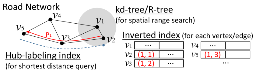
Figure 2: Index structure.

4.3 Filtering with Temporal Information

As mentioned in § 2.3, we can treat any kind of temporal constraints as postprocessing. For interval constraints, such as $[T_{i},T_{j}]\subseteq I$ or $[T_{i},T_{j}]\cap I\neq\emptyset$, we can prune candidates before verification as follows. For each candidate trajectory $(P^{(id)},T^{(id)})$ of length $n$, we check its first and last timestamps (i.e., $I^{(id)}:=[T_{1}^{(id)},T_{n}^{(id)}]$). Given a query time interval $I$, if $I^{(id)}\cap I=\emptyset$, then we have $[T_{i},T_{j}]\not\subseteq I$ and $[T_{i},T_{j}]\cap I\neq\emptyset$; we can safely prune this candidate. Furthermore, depending on the application, we may sort the records in each postings list by their temporal information such as departure time (i.e., $T^{(id)}_{1}$) or maximum speed (i.e., $\max_{1\leq t\leq|T^{(id)}|-1}w(P_{t}^{(id)})/(T^{(id)}_{t+1}-T^{(id)}_{t})$, where $w(e)$ is the distance of an edge $e$). This allows us to generate candidates with binary search on postings lists, hence to avoid those violating the temporal constraint.

5 Verification

The generated candidates usually include many false positives; therefore, we need to verify them efficiently to obtain the answer. Existing methods for whole matching similarity search (e.g., [48, 64]) computes the similarity between $P$ and $Q$ with dynamic programming (DP) for each candidate. Similarly, in our subtrajectory search setting, we can compute the similarity by sequentially filling a $|P|\cdot|Q|$ matrix based on the recursive definition of WED, which is referred to as the Smith-Waterman (SW) algorithm. The time complexity is $O(|P|\cdot|Q|)$, as shown in Figure 3(a). This naive SW algorithm includes the following redundant computation: (1) Although a subtrajectory of $P$ similar to $Q$ can be a small part of $P$, the SW algorithm computes DP matrix for the entire $P$. (2) If two trajectories share a subtrajectory, the DP matrices have common values, but the SW algorithm does not exploit this property.

Main Idea.  We reduce redundant computation as follows. (1) Local verification: Given a candidate $(id,j,i_{q})$, the subtrajectory similar to $Q$ are located around the position $j$ of $P$; hence we only need to run DP around $j$. (2) Trie-based caching: We share computation for common subtrajecories by exploiting the sparsity of a road network: Although the alphabet $\Sigma$ is large, the possible previous/next symbols of $P_{j}$ (i.e., $P_{j-1}$ and $P_{j+1}$) are limited because trajectories move along physically connected vertices (edges) in a road network; hence we can efficiently cache the columns of DP matrices.

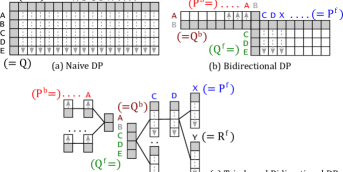
Figure 3: Comparison of verification methods ($P=$ ABCDX…, $Q=$ ABCDE; colors show partition).

5.1 Local Verification

The filtering phase gives $(id,j,i_{q})$, where $j$ is a position such that $P^{(id)}_{j}$ matches $Q_{i_{q}}$ or its substitution neighbor. The local verification is to check if there exists a subtrajectory $P_{s:t}^{(id)}$ such that $\textsf{wed}(P_{s:t}^{(id)},Q)<\tau$, where $s\leq j\leq t$. Our idea is to run the DP computation from $j$ bidirectionally. To guarantee that we will not miss any similarity search result after verifying all the candidates, we have the following lemma.

Lemma 1.

Given a subtrajectory $P_{s:t}^{(id)}$ of $P$ such that $\textsf{wed}(P_{s:t}^{(id)},$ $Q)$ $<\tau$, and the set of candidates $\mathcal{C}$ identified by subsequence filtering, there exists $(id,j,i_{q})\in\mathcal{C}$ such that $s\leq j\leq t$ and

$$\textsf{wed}(P_{s:t}^{(id)},Q)=\; \textsf{wed}(P_{s:j-1}^{(id)},Q_{1:i_{q}-1})+\textsf{sub}(P_{j}^{(id)},Q_{i_{q}})$$

$$+\textsf{wed}(P_{j+1:t}^{(id)},Q_{i_{q}+1:|Q|}).$$ (10)

This lemma suggests that for every subtrajectory that satisfies the WED constraint, we can always find a position $j$ in the candidates identified by subsequence filtering, such that $P_{j}^{(id)}$ is aligned to $Q_{i_{q}}$ in the optimal alignment that yields the WED. Thus, we can verify from $j$ to obtain the similarity search result. Specifically, by Eq. (10), we partition $P_{s:t}^{(id)}$ into three parts at $j$ and compute WED bidirectionally [15]. From $j$, we run two DPs: a backward one (i.e., from the end of strings to the start) for $\textsf{wed}(P_{s:j-1}^{(id)},Q_{1:i_{q}-1})$ and a forward one for $\textsf{wed}(P_{j+1:t}^{(id)},Q_{i_{q}+1:|Q|})$. By iterating $s$ from $j$ to $1$ and $t$ from $j$ to $|P^{(id)}|$ in the two DPs, respectively, we are able to find all $P_{s:t}^{(id)}$ such that $s\leq j\leq t$ and $\textsf{wed}(P_{s:t}^{(id)},Q)<\tau$. The above step is conducted for each $(id,j,i_{q})$ in the candidate set to obtain all the similarity search results. For ease of exposition, in the rest of this section, we omit the superscript $(id)$ from $P$, and we use $P^{b}$ to denote $P_{s:j-1}$ and $P^{f}$ to denote $P_{j+1:t}$.

Example 8.

Consider a trajectory $P=...\textsf{ABCDX}...$ and a query $Q=\textsf{ABCDE}$. Assume a $\tau$-subsequence is $Q^{\prime}=\{\textsf{B}\}$ and there is only one candidate whose $j=2$ and $i_{q}=2$. As shown in Figure 3(b), we partition $P$ into $(P^{b},P_{j},P^{f})=(...\textsf{A},\textsf{B},\textsf{CDX}...)$ and $Q$ into $(Q^{b},Q_{i_{q}},Q^{f})=(\textsf{A},\textsf{B},\textsf{CDE})$. We can find all subtrajectories $P_{s:t}$ such that $s\leq 2\leq t$ and $\textsf{wed}(P_{s:t},Q)<\tau$ by computing $\textsf{sub}(\textsf{B},\textsf{B})+\textsf{wed}(...\textsf{A},\textsf{A})+\textsf{wed}(\textsf{CDX}...,\textsf{CDE})$.

Early Termination. For each direction $d\in\{b,f\}$, we can terminate the computation before reaching the end of $P^{d}$. Given a position $0\leq k\leq|P^{d}|$ ($k=0$ for the case of an empty string), by the definition of WED, we have the following lower bound of the WED between $P^{d}$ and $Q$:

$$LB_{k}^{d}:=\min_{0\leq j\leq|Q|}\{\textsf{wed}(P_{1:k}^{d},Q_{1:j})\}\leq\textsf{wed}(P^{d},Q).$$ (11)

If the lower bound for any $k$ reaches $\tau$, we can safely terminate the DP computation of $P^{d}$.

5.2 Caching with Bidirectional Trie

The local verification still involves redundant computation when we verify multiple candidates. We begin with an example.

Example 9.

(Continuing from Example 8) Consider another trajectory $R=...\textsf{ABCDY}...$ identified as a candidate via B. In the local verification, we need to compute both $\textsf{wed}(P^{f},Q^{f})$ and $\textsf{wed}(R^{f},Q^{f})$, where $Q^{f}=\textsf{CDE}$, $P^{f}=\textsf{CDX}...$, and $R^{f}=\textsf{CDY}...$. Hence, when computing $\textsf{wed}(P^{f},Q^{f})$ and $\textsf{wed}(R^{f},Q^{f})$, the first two columns of the DP matrices share the same values because $P^{f}$ and $R^{f}$ has a common prefix CD. This indicates that we can reduce the computation by caching these columns.

In general, given a vertex/edge in the road network, the number of possible next vertices/edges are very small (typically, three) compared to the alphabet size because of the structure of the road network. This implies that the candidate subtrajectories starting from $Q_{i_{q}}$ tend to share a prefix; therefore, we expect that the caching strategy will improve the efficiency.

To efficiently cache the DP columns of common prefixes, we employ a trie-based data structure as shown in Figure 3(c). We describe how this trie works using a running example.

Example 10.

(Continuing from Example 9) After computing $\textsf{wed}(P^{f},Q^{f})$, we have three columns corresponding to C, D, and X, as in Figure 3(c). When computing $\textsf{wed}(R^{f},Q^{f})$, we can reuse the two columns for C and D that are cached in the trie.

As candidates tend to have common prefixes as discussed above, we expect that the cache miss rate is low and the verification gets faster. A trie is built for each direction (hence called a bidirectional trie) and each symbol in the $\tau$-subsequence of $Q$. So there are $2|Q^{\prime}|$ tries.

5.3 Verification Algorithm

Algorithms 3–6 summarize our verification algorithm. First, for each direction $\{b,f\}$ and $q\in Q^{\prime}$ where $Q^{\prime}$ is a $\tau$-subsequence of $Q$, empty tries are initialized (each trie is denoted by $\mathcal{T}_{i_{q}}^{b}$ or $\mathcal{T}_{i_{q}}^{f}$, where $i_{q}$ indicates the candidate position in $Q$). Then, for each candidate $(id,j,i_{q})\in\mathcal{C}$, VerifyCandidate (Algorithm 4) is applied and the results are stored in $\mathcal{A}$.

In VerifyCandidate, the data trajectory $P$ and query $Q$ are partitioned into three parts. Then, for each direction $d\in\{b,f\}$, AllPrefixWED is called to compute an array $E^{d}$, whose $k$-th element is the WED between $Q^{d}$ and the $k$-th prefix of $P^{d}$, i.e., $E_{k}^{d}=\textsf{wed}(P^{d}_{1:k},Q^{d})$. We can use a tighter threshold $\tau^{\prime}:=\tau-\textsf{sub}(q,b)$ instead of the original $\tau$ because of Eq. (10); this $\tau^{\prime}$ is used for early termination. Finally, all the subtrajectories that satisfy Eq. (10) $<\tau$ are added to the result set.

In AllPrefixWED (Algorithm 5), we compute the array $E^{d}$. A symbol $c$ in a given trajectory $P^{d}$ is processed one by one; if a child node corresponding to $c$ at the current trie is found (Line 3), we skip computing the corresponding DP column; otherwise, we create a new child (Line 5) and compute the DP column (Line 6) using the StepDP procedure (Algorithm 6), a standard DP that computes a new column based on the previous column. $A^{(x)}$ represents a DP column cached in the trie node $x$. By Eq. (11), if the lower bound $LB_{k}^{d}$ exceeds a given threshold (Line 7), we can safely terminate the DP computation for $P^{d}$. Finally, the value $A_{|Q_{d}|}^{(x)}=\textsf{wed}(P^{d}_{1:k},Q^{d})$ is stored to $E_{k}^{d}$ (Line 9).

input : Candidates $\mathcal{C}$; Query $Q$; Threshold $\tau$

1 for $(q,i_{q})\in Q^{\prime}$ do

2       $\mathcal{T}_{i_{q}}^{f}\!,\mathcal{T}_{i_{q}}^{b}\!\leftarrow\text{Empty tries}$

3for $(id,j,i_{q})\in\mathcal{C}$ do

4       $\mathcal{A}\leftarrow\mathcal{A}\cup\textsf{VerifyCandidate}(Q,(id,j,i_{q}),\tau,\mathcal{T}_{i_{q}}^{f},\mathcal{T}_{i_{q}}^{b})$

return $\mathcal{A}$

Algorithm 3 $\textsf{Verify}(\mathcal{C},Q,\tau)$

input : Query: $Q\in\Sigma^{*}$; Candidate: $(id,j,i_{q})$; Threshold: $\tau$; Forward/Backward tries: $\mathcal{T}^{f},\mathcal{T}^{b}$

1 $P\leftarrow\textsf{accessTrajectory}(id)$

$(P^{b},b,P^{f})\leftarrow(P_{1:(j-1)},P_{j},P_{(j+1):|P|})$

  $\triangleright$ Partition

$(Q^{b},q,Q^{f})\leftarrow(Q_{1:(i_{q}-1)},Q_{i_{q}},Q_{(i_{q}+1):|Q|})$

  $\triangleright$ Partition

2 $E^{b}\leftarrow\textsf{AllPrefixWED}(Q^{b},P^{b},\tau^{\prime},\mathcal{T}^{b}\!.\textsf{root})$

3$E^{f}\leftarrow\textsf{AllPrefixWED}(Q^{f},P^{f},\tau^{\prime},\mathcal{T}^{f}\!.\textsf{root})$

4for $(s,t)$ such that $\textsf{sub}(q,b)+E^{b}_{s}+E^{f}_{t}<\tau$ do

      $\mathcal{S}\leftarrow\mathcal{S}\cup\{(id,s,t)\}$

        $\triangleright$ Initialized as $\mathcal{S}=\emptyset$

5      

return $\mathcal{S}$

  $\triangleright$ All subtrajectories $P_{s:t}$ that matches $Q$

Algorithm 4 $\textsf{VerifyCandidate}(Q,(id,j,i_{q}),\tau,\mathcal{T}^{f},\mathcal{T}^{b})$

input : Query $Q^{d}$; Trajectory $P^{d}$; Trie node $x$; ($d\in\{f,b\})$

output : WED between $Q^{d}$ and $P^{d}_{1:k}$ $(\forall k)$

$E^{d}\leftarrow\text{Empty array}$

  $\triangleright$ $E_{k}^{d}$ means $\textsf{wed}(Q^{d},P^{d}_{1:k})$

1 for $k$ in $1..|P^{d}|$ do

2       $c:=P^{d}_{k}$;   $x_{\textsf{parent}}\leftarrow x$;    $x\leftarrow x_{\textsf{parent}}.\textsf{findChild}(c)$

3       if $x$ not found then

             $x\leftarrow x_{\textsf{parent}}.\textsf{createChild}(c)$

              $\triangleright$ New child

             $A^{(x)}\leftarrow\textsf{StepDP}(Q^{d},c,A^{(x_{\textsf{parent}})})$

              $\triangleright$ Fill DP column

4            

5      

6      if $\tau\leq\min_{0\leq j\leq|Q|}A_{j}^{(x)}\;(=LB_{k}^{d})$ then

            break

              $\triangleright$ Early Termination (Sec.5.1)

7            

      $E_{k}^{d}\leftarrow A^{(x)}_{|Q^{d}|}$

        $\triangleright$ $\textsf{wed}(Q^{d},P^{d}_{1:k})$

8      

return $E^{d}$

Algorithm 5 $\textsf{AllPrefixWED}(Q^{d},P^{d},\tau,x)$

input : Query $Q^{d}$; Next symbol $p\in\Sigma$; DP array $A_{0:|Q^{d}|}$

1 $B\leftarrow$ Array of length $|Q^{d}|+1$;    $B_{0}\leftarrow A_{0}+\textsf{del}(p)$

2 for $j$ in $1..|Q^{d}|$ do

3       ​$B_{j}\!\leftarrow\!\min\{A_{j-1}\!+\!\textsf{sub}(p,Q^{d}_{j}),A_{j}\!+\!\textsf{del}(p),B_{j-1}\!+\!\textsf{ins}(Q^{d}_{j})\}$

return $B$

Algorithm 6 $\textsf{StepDP}(Q^{d},p,A)$

6 Experiments

6.1 Settings

Evaluation was conducted on the following datasets: Beijing (T-drive) [65], Porto [31], Singapore [44], and SanFran [4]. For Beijing and Porto, we conducted map matching [34] to obtain network-constrained representation. SanFran is a large synthesized dataset by the moving object generator [4] with the San Francisco road network. The statistics after preprocessing are presented in Table 2.

Table 2: Dataset statistics.

Dataset	# Trajectories	Avg. Length	$|V|$	$|E|$
Beijing	786,801	101	86,484	171,135
Porto	1,701,238	81	75,265	135,133
Singapore	287,524	262	18,127	48,236
SanFran	11,505,922	101	175,343	223,606

Our method consists of the (optimized) subsequence filtering with the bidirectional trie (BT) verification (referred to as OSF-BT). We also consider OSF-SW, where BT is replaced by the Smith-Waterman (SW) algorithm for verification. Further, we compare with the following baselines.

DISON.  DISON [64] is a whole matching method for LCRS. We adapted it to our problem. Since the early termination technique in [64] does not work here, we used SW (DISON-SW) or BT verification (DISON-BT).

Torch.  Torch [48] is a whole matching method that supports several similarity functions. We adapted it to our problem. We equipped it with SW (Torch-SW) and BT (Torch-BT) for verification. The upper bounding technique [48] prior to verification was developed for LORS and does not apply here.

DITA.  DITA [41] is a whole matching method developed for DTW and can be adapted for other functions. We modified its pivoting method to fit WED. Since DITA does not support subtrajectory search, we enumerated all subtrajectories and indexed them. Note the enumeration is done offline and not counted towards query processing time. We used SW instead of the double-direction verification (DDV) [41] because DDV works for DTW but does not improve upon SW for WED.

$q$-gram indexing for EDR.  $q$-gram indexing was proposed in [7] for whole matching under the EDR based on the fact that if there are less than $\max\{|P|,|Q|\}-q+1-\tau q$ common $q$-grams between $P$ and $Q$, then $\textsf{EDR}(P,Q)>\tau$. We customized their method to support subtrajectory search under EDR. We set $q=3$. SW was used for verification.

Indexing for ERP.  ERP-index was proposed in [6]. It employs lower bounding and triangle inequality. Given a sequence $P$ of coordinates, we indexed the sum of all coordinates, $sum(P)\in\mathbb{R}^{2}$, in a spatial index (we used $k$d-tree). Given a query sequence $Q$, $\|sum(P)-sum(Q)\|$ gives a lower bound. We enumerated and indexed all subtrajectories. SW was used for verification.

Smith-Waterman (SW).  The SW algorithm [43] is a non-indexing method for substring matching. We adopted it (referred to as Plain-SW) to process all the data trajectories.

Since DITA and ERP-index enumerate all subtrajectories, the whole datasets are impossible to index due to exceeding the main memory (e.g., Beijing dataset generated 1.4 billion subtrajectories). We used a fraction of the dataset when these two methods were included in the competitors.

We used the six WED instances introduced in § 2.2 as similarity functions. Instead of specifying a similarity threshold $\tau$ directly, we used a threshold ratio $\tau_{\textsf{ratio}}\in[0,1]$. Given a query $Q$ and $\tau_{\textsf{ratio}}$, we set $\tau:=\tau_{\textsf{ratio}}\sum_{q\in Q}c(q)$. We used $\tau_{\textsf{ratio}}=0.1$ as the default value. For SURS, LORS, and LCRS, costs are given by road lengths. The cost functions of the other WED instances are given in § 2.2. For EDR, we used $\varepsilon=0.001$. For NetEDR, we set $\varepsilon$ to the median distance of edges in $E$. For NetERP deletion cost $G^{\textsf{(del)}}_{\textsf{NetERP}}$, we used $2M$. For $\eta$ in Eq. (5), we used $\eta=0$ for Lev, EDR, SURS, and NetEDR, $10^{-4}$ multiplied by the median distance of a node and its nearest neighbor for ERP, and the median road length for NetERP (see Appendix D for the choice of $\eta$).

All evaluations were conducted on a workstation with Intel Core i9-7900X CPU (3.30GHz) and 64GB RAM. All methods were implemented in C++ (g++ v.7.3.0) with the -O3 option. We do not use multi-threading (for distributed baselines, we implemented centralized versions to compare algorithms themselves). All the algorithms were implemented in a main memory fashion.

6.2 Effectiveness

6.2.1 Travel Time Estimation

To demonstrate the effectiveness of WED and subtrajectory similarity search, we first consider an on-the-fly travel time estimation task following the approach in [53]. We use the Beijing dataset and sample 130 queries of length 60, where the numbers of exact match are less than 10 (i.e., the sparse case). The travel times corresponding to the subtrajectories that exactly match the query $Q$ are used as ground truth data. For estimation, we find the subtrajectories $\{P^{(id)}_{i:j}\}$ in the database similar to $Q$ under a threshold $\tau_{\text{ratio}}$. Since a trajectory $P^{(id)}$ may have multiple subtrajectories similar to $Q$, we pick the most similar one and break tie by the shortest one. Then we compute the average of the travel time, $T^{(id)}_{j}\!\!-T^{(id)}_{i}$, over those similar to $Q$ as the estimated value. In order to evaluate the superiority of similarity search over exact match, we measure mean squared errors (MSEs) and report the relative value ($RMSE:=MSE(\tau_{\text{ratio}})/MSE(\text{exact})$). Since the ground truths are contained in both results of similarity search and exact match, we employ a leave-one-out cross-validation  by excluding one ground truth from the result set at a time. RMSE $<100\%$ means similarity search is better than exact match.

We compare the six WED instances in § 2.2 with DTW, LORS, LCRS, and LCSS. Since LORS, LCRS, and LCSS are defined on shared road segments, we convert them to equivalent distance functions. DTW, LORS and LCSS are normalized to $[0,1]$ such that $\textsf{DTW}(P,Q)\leq\tau_{\text{ratio}}\sum_{i=1}^{|Q|-1}d(Q_{i},Q_{i+1})^{2}$ and $\textsf{LORS}(P,Q)\geq(1-\tau_{\text{ratio}})\cdot\sum_{i=1}^{|Q|}w(Q_{i})$ (the same for LCSS). Figure 4 shows how the RMSE changes over $\tau_{\text{ratio}}$ (LORS and LCSS have RMSE $>100\%$ at $\tau_{\text{ratio}}=0$ because they do not count mismatching road segments in $P^{(id)}$). For most WED instances, similarity search performs better than exact match when $\tau_{\text{ratio}}\in[0.04,0.14]$, showcasing the superiority of similarity search for travel time estimation on sparse data. To compare similarity functions, all the WED instances except ERP perform well, while LORS and LCSS deliver the worst performance. SURS achieves the smallest RMSE (89%) among all the similarity functions. NetEDR and NetERP are competitive when $\tau_{\text{ratio}}$ is large. These observations suggest that WED is useful for travel time estimation and these new WED instances are better than existing ones (Lev, EDR, and ERP). We also observe that LCRS and SURS behave similarly because of similar semantics. An advantage of SURS over LCRS is that efficient subtrajectory search under LCRS has not been established and thus we enumerate all subtrajectories ($O(\sum_{k=1}^{N}|P|^{2}|Q|)$-time), while SURS belongs to WED and can be efficiently processed. Next, we compare similar subtrajectory matching with whole matching. Since whole matching finds no result for most thresholds, we consider a top-$k$ setting for fair comparison. The RMSE is reported in Table 3 for SURS, the best function in the previous experiment. The result shows that the RMSE of subtrajectory matching is about half of the RMSE of whole matching, and the gap is more significant for small $k$.

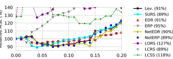
Figure 4: RMSE of travel time estimation (Beijing), best values reported on the right side.

Table 3: RMSE of travel time (SURS, Beijing).

$k$	$5$	$10$	$15$	$20$	$25$
Subtrajectory	92 %	91 %	102 %	108 %	116 %
Whole	233 %	221 %	219 %	220 %	220 %

6.2.2 Alternative Route Suggestion

Next we show the effectiveness through an alternative route suggestion task. Suppose a driver is planning to travel from an origin $u$ to a destination $v$ through a route $Q$, and the driver wants to find if there are variations of $Q$ as alternative routes. We can do this by retrieving subtrajectories from $u$ to $v$ similar to $Q$ from the database. To measure the preference of a route, we employ the route naturalness described in [66] §7: drivers prefer routes that go directly towards the destination, and the log-likelihood of a route is proportional to the number of hops that get closer (in terms of road network distance) to the destination than ever. Following this idea, given a route $P$ such that $P_{1}=u$ and $P_{|P|}=v$, we define its naturalness as the ratio of hops that get closer to $v$ than ever, i.e., $\frac{|C|}{|P|-1}$, where $C=\{(P_{i-1},P_{i})\mid\min_{1\leq j<i}d(P_{j},v)>d(P_{i},v)\}$. If a route includes many inefficient detours, then the naturalness is low.

Figure 5 shows the naturalness of the routes suggested by subtrajectory similarity search under various similarity functions. The results are averaged over 3,000 queries uniformly sampled from the Beijing dataset. We vary $\tau_{\text{ratio}}$ from 0 to 0.3 at 0.05 interval and plot the cardinality (i.e., the number of suggested routes) and the naturalness. The cardinality increases w.r.t. $\tau_{\text{ratio}}$, but the rate depends on the similarity function. So we do not show $\tau_{\text{ratio}}$ explicitly. Among the six WED instances, Lev, EDR, NetEDR, and NetERP deliver routes with high naturalness. LCSS, LORS, and LCRS exhibit low naturalness because they measure common road segments but do not penalize inefficient detours. DTW’s naturalness is high for short queries but drops rapidly for long queries. Another interesting observation is that when query length is 50 or 60, the naturalness using WED instances, except ERP, first decreases w.r.t. the cardinality and then rebounds. This is because some highly natural routes involve shortcuts that are spatially distant from the queries. They cause large DTW or ERP and hence are not identified using the two functions, while the WED instances with non-spatial distance as costs are capable of capturing these routes.

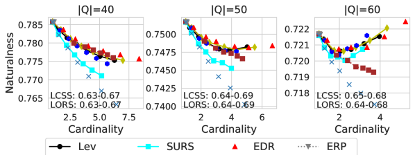
Figure 5: Naturalness of alternative routes suggested by similarity search $\tau_{\text{ratio}}\in[0,0.3]$ (Beijing).

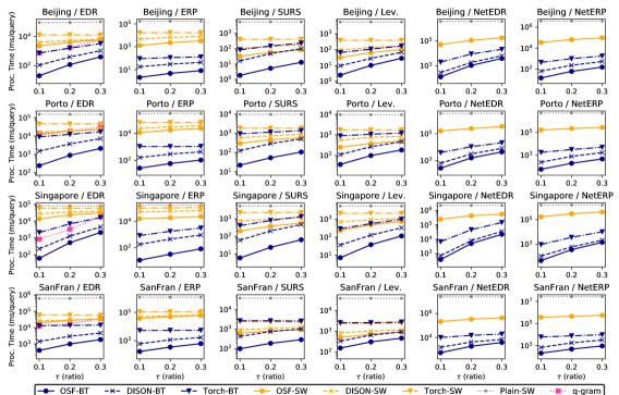
Figure 6: Varying $\tau_{\textsf{ratio}}$: OSF-BT is our method (legend is shown at the bottom).

6.3 Query Processing Time

Following past related studies [51, 53, 22, 20], we randomly sampled subtrajectories from each dataset as queries. We set the default query length $|Q|$ to 60, whose path distance in real world ranges from 500 m to 40 km, with an average of 6.5 km, in line with [51, 53, 59]. Evaluation metrics were averaged over 100 queries, except for Plain-SW, whose processing time was averaged over 10 queries due to the computational cost.

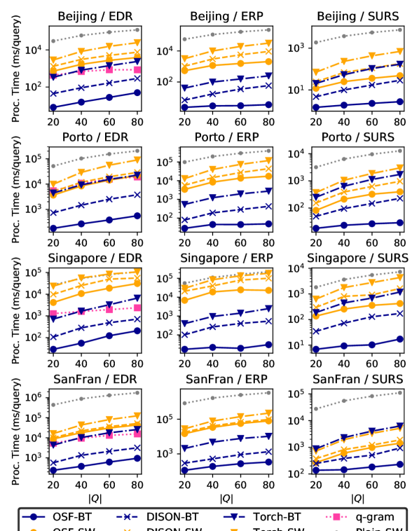
Figure 7: Varying $|Q|$.

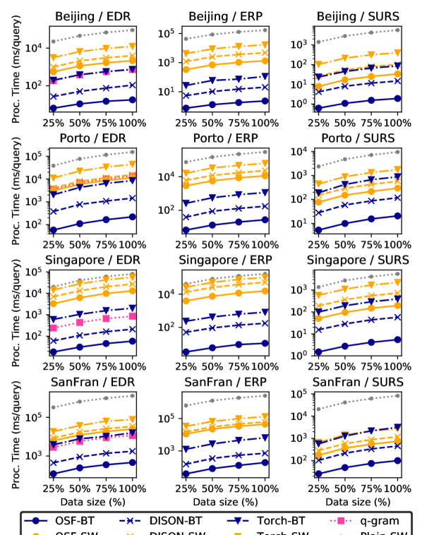
Figure 8: Varying $\mathcal{T}$.

Table 4: Running time breakdown (ms).

		Varying $\tau_{\textsf{ratio}}$		Varying $|Q|$
	Default†	0.2	0.3	20	40
MinCand	0.002	0.005	0.007	0.0005	0.001
Index lookup	0.070	0.259	0.443	0.039	0.055
Verify	19.9	113.1	390.0	6.2	11.1

• Default: $\tau_{\text{ratio}}=0.1$, $|Q|=60$, dataset size $=100\%$.

We first investigate the effect of the similarity threshold $\tau_{\text{ratio}}$. Figure 6 shows that the proposed method OSF-BT outperforms the other competitors. It responses in less than 2 seconds except for NetEDR, and typically hundreds of milliseconds when $\tau_{\text{ratio}}=0.3$. Compared to DISON-BT and Torch-BT, which employ different filtering principles, our OSF-BT always performs better and is up to 9 times faster than DISON-BT and 73 times faster than Torch-BT. Comparing our BT verification with SW, BT significantly improves the efficiency. The impact of BT is more significant for NetEDR and NetERP, which involve relatively expensive computation in verification. For this reason, we omitted the results of DISON-SW and Torch-SW for NetEDR and NetERP from Figure 6, which take at least 24 hours for computation for 100 queries. These results indicate that both OSF and BT improve the performance, and improvements are consistently observed whatever similarity function is used.

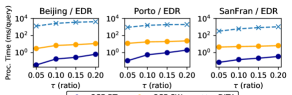
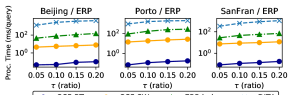
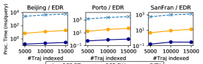
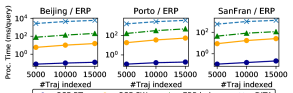
Figure 9: Comparison with baselines involving subtrajectory enumeration (Varying $\tau_{\text{ratio}}$; $|\mathcal{T}|=5000$; EDR/ERP).

Figure 10: Comparison with baselines involving subtrajectory enumeration (Varying $|\mathcal{T}|$; $\tau_{\text{ratio}}=0.1$; EDR/ERP).

We vary the length of query $|Q|$ with $\tau_{\text{ratio}}=0.1$. As shown in Figure 8, OSF-BT is always faster than the others. For larger $|Q|$, the processing time of OSF-BT increases as well as the other methods. The reason is two-fold: (1) the verification cost is proportional to $|Q|$; (2) in our setting, the similarity threshold $\tau$ increases as $|Q|$ increases, making the candidate set larger.

In Table 4, we decompose the query processing time of OSF-BT (on Beijing, EDR) to: MinCand computation, index lookup, and verification. Most time (around 99%) is spent on verification, whose time increases with $\tau_{\text{ratio}}$ and $|Q|$. This is expected, because for each candidate we need only one index lookup but run a quadratic-time DP to verify it. MinCand computation is almost negligible since it runs in $O(|Q|^{2})$ time, which does not depend on the dataset size.

Figure 8 shows query processing time when we vary the dataset size. All the methods scales linearly and OSF-BT is consistently the fastest. In addition, we show results for DITA and ERP-index, which requires subtrajectory enumeration, on a fraction of the datasets where they can fit into the main memory; e.g., in order to store the randomly chosen 5,000 trajectories, the number of subtrajectories to be indexed is 48M (Beijing), 37M (Porto), and 26M (SanFran). The query processing time for this small dataset is shown in Figure 10 (varying $\tau_{\text{ratio}}$) and Figure 10 (varying dataset size). Our method outperforms DITA and ERP-index by two orders of magnitude. This result indicates that applying whole matching methods to subtrajectory matching by enumerating all subtrajectories is impractical for large datasets.

6.4 Filtering and Verification

We compare the filtering power by evaluating the candidate size $|\mathcal{C}|$. Note for all the competitors the candidates are in the form of $(id,j,i_{q})$ for fair comparison. Figure 11 shows: (1) OSFconsistently results in the best filtering power; its candidate size is on average 3.4, 2.9, and 25 times smaller than DISON, $q$-gram, and Torch, respectively. (2) OSFshows good scalability against $|Q|$, because for long $|Q|$, the item set in MinCand becomes large and thus the probability of including “good-value-for-the-price” items becomes large. We also compare with DITA and ERP-index on a fraction of the datasets. Their candidate sizes are on average 105 and 14 times OSF’s, respectively.

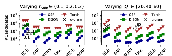
Figure 11: Number of candidate positions (Beijing).

To separate the effect of local verification (§ 5.1) and the effect of caching with BT (§ 5.2), we evaluate (i) unpruned position rate (UPR), and (ii) cache miss rate (CMR), which are respectively defined as (i) the rate of DP columns that pass the early termination (§ 5.1) compared to SW, and (ii) the rate of DP columns where the StepDP procedure is actually called among the DP columns that pass the early termination. Table 5 shows results for the Beijing dataset under EDR. We observe both local verification and BT contribute to pruning. The rates increase with $\tau_{\textsf{ratio}}$ and $|Q|$ due to looser similarity constraint and longer query to verify, but decrease with dataset size due to more shared prefixes/suffixes. The total unpruned rate (TUR), defined by $\text{UPR}\times\text{CMR}$, shows small values, indicating the number of StepDP calls is far less than that by SW.

Table 5: Evaluation of verification (%).

		Varying $\tau_{\textsf{ratio}}$		Varying $|Q|$		Varying $|\mathcal{T}|$
	Default†	0.2	0.3	20	40	25%	50%
UPR	21.89	52.05	94.28	6.57	14.45	23.15	22.65
CMR	2.19	4.72	7.50	0.35	1.13	4.43	2.99
TUR	0.48	2.46	7.07	0.02	0.16	1.02	0.68

• Default: $\tau_{\text{ratio}}=0.1$, $|Q|=60$, dataset size $=100\%$.

6.5 Index Construction Time / Index Size

Table 6 the index construction time and index size. The index construction time of our postings lists is relatively fast. For reference, we show results for methods involving subtrajectory enumeration (ERP-index and DITA). Although these are results with only 5,000 trajectories, the index construction time and index size are larger than ours except on the SanFran dataset.

Table 6: Index construction time / index size.

	Beijing	Porto	SanFran
OSF-BT†	7s / 0.59 gb	10s / 1.02 gb	79s / 8.63 gb
$q$-gram	15s / 0.59 gb	19s / 1.01 gb	269s / 8.55 gb
$\downarrow$ Tiny dataset
(ERP-index${}^{\dagger\!\dagger}$)	23s / 2.6 gb	17s / 1.9 gb	14s / 1.4 gb
(DITA${}^{\dagger\!\dagger}$)	60s / 1.79 gb	36s / 0.71 gb	31s / 0.15 gb

• DISON and Torch have the same time/size as OSF-BT.

• Reference values with only 5,000 trajectories. DITA construction depends on the similarity function. Here we showed a result for ERP.

6.6 Temporal Constraints

We show the results with temporal constraints of type $[T_{i},T_{j}]\cap I\neq\emptyset$, where $I$ is a query time interval. We vary temporal selectivity (e.g., 1% temporal selectivity means $I=[ts_{\min},ts_{1\%}]$, where $ts_{\min}$ is the minimum timestamp and $ts_{1\%}$ is the 1% quantile). For pruning, temporal constraints are checked after candidate generation (referred to as TF, see § 4.3). With this pruning, the processing time scales almost linearly with temporal selectivity. We compare with the method that checks temporal constraints as postprocessing (no-TF). Figure 12 shows that TF is faster by one order of magnitude. The gap is more significant when temporal selectivity is low.

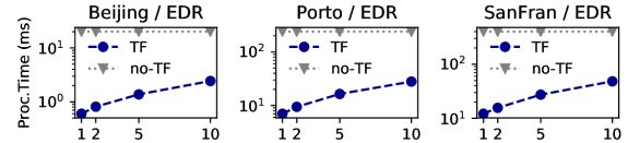
Figure 12: Varying temporal selectivity (TS).

7 Related Work

Trajectory Similarity Functions.  Trajectory similarity functions can be classified into: (1) coordinate-aware similarity functions are defined based on spatial coordinates of trajectories [63, 42, 7, 6, 58, 66] and (2) network-aware similarity functions employ network features, such as travel costs [39, 40, 48, 55, 56, 11, 14, 46, 64]. Coordinate-aware similarity functions include dynamic time warping (DTW), edit distance with real penalty (ERP) [6], edit distance on real sequence (EDR) [7], edit distance with projections (EDwP) [37], and Fréchet distance. Their pros and cons were investigated in [48, 7, 6, 64, 45]. ERP and EDR are WED instances. DTW, EDwP, and Fréchet distance are not. Recent effort aimed to learn deep trajectory representations [27] or metrics [62] to reduce the computation of similarity to linear time. For network-aware similarity functions, a natural way is to measure the shared or unshared edges. Weighted Jaccard distance [56] and weighted Dice distance [55] are order-insensitive functions (i.e., edge ordering not incorporated). Longest common subsequences (LCSS) [47, 32], Longest overlapping road segments (LORS) [48], and longest common road segments (LCRS) [64] are order-sensitive functions, while they do not belong to WED . Another strategy is to incorporate shortest path distances between vertices [39, 40, 11, 14, 46].

Trajectory Indexing.  Although much attention has been gathered to indexing for non-constrained trajectories (see surveys [30, 35]), indexing methods for trajectories in road networks are also studied actively [9, 22, 21, 20, 48, 64]. Chen et al. proposed ERP [6] and EDR [7] along with the query processing algorithms. Wang et al. [48] and Yuan and Li [64] proposed algorithms to support various similarity functions but they were designed for whole matching (though can be adapted for subtrajectories, see our experiments). Furthermore, their filtering policies are different from ours (based on scanning postings lists for all symbols [48] or prefix symbols [64] of a query). Shang et al. [41] and Xie et al. [58] proposed distributed systems for similarity search under DTW and discrete Fréche/Hausdorff distances, respectively. These methods [41, 58] support only whole matching. Pivot points were proposed in [41] for pruning. The differences from our method are: (1) The pivots are selected by turning points or the distance to neighbor points/origin/destination, while our $\tau$-subsequence is chosen by a selectivity optimization algorithm. (2) In contrast to pivot points, our filtering is designed towards the general case of WED, and thus does not require individual adaptation for specific similarity functions.

String / Time-series Similarity Search.  Edit distance has been employed for string similarity search. Bouding techniques (e.g., by $q$-grams [36, 10, 54]) are widely used. In bioinformatics, three types of similarity search methods are used: global [33], local [43, 26, 60], and semi-global alignments [25]. The Smith-Waterman algorithm [43] can be used for WED. Trajectories also belong to time series data, whose similarity is often measured by Euclidean distance, DTW, ERP, or LCSS. Common indexing methods are based on lower bounding [3, 17]. Substring similarity search can be carried out by indexing methods based on suffix arrays (or suffix-tries) [26, 19]. Our BT method can be regarded as a method that dynamically builds prefix- and suffix-tries for verification instead of a static trie.

8 Conclusion and Future Work

We tackled subtrajectory similarity search under WED, a class of similarity function that includes several important similarity functions. For efficient search, we proposed subsequence filtering, which involves a discrete optimization problem to choose the optimal subsequence. Based on this technique, we developed an algorithm using filter-and-verify strategy. We designed a local verification method equipped with bidirectional tries. We showed the effectiveness of WED and the superiority of our solution over alternative methods. Interesting future directions include supporting more general class of similarity functions, developing a distributed indexing method, and more sophisticated treatment of temporal information. Acknowledgments.  This work was supported by JSPS 16H01722, 17H06099, 18H04093, 19K11979, and NSFC 61702409.

Appendix A Pseudo-codes

Algorithm 7 describes the SW algorithm for finding the best substring $P_{s,t}\sqsubseteq P$ that minimizes $\textsf{wed}(Q,P_{s:t})$. The minimum operation at Line 8 is taken based on the first elements, i.e., $(a,b,c)$. Note that the matrix $K$ memorizes the first subscript $s$ of the current best substring; this technique was used in [38].

input : Query $Q\in\Sigma^{*}$; Trajectory $P\in\Sigma^{*}$

output : The best matching substring $P_{s:t}$ with $\textsf{wed}(Q,P_{s:t})$

1 $D,K\leftarrow(|Q|+1)\times(|P|+1)$ zero matrices

2 $D_{i,0}\leftarrow\sum_{i^{\prime}=1}^{i}\textsf{del}(P_{i^{\prime}})$  ($1\leq i\leq|Q|$)

3 $\textit{BestSoFar}\leftarrow\infty$

4 for $j$ in $1..|P|$ do

5       $K_{0,j}\leftarrow j$

6       for $i$ in $1..|Q|$ do

7             $(a,b,c)\leftarrow(D_{i-1,j-1}+\textsf{sub}(Q_{i},P_{j}),D_{i-1,j}+\textsf{del}(P_{j}),D_{i,j-1}+\textsf{ins}(Q_{i}))$

8             $(D_{i,j},K_{i,j})\!\leftarrow\!\min\{(a,K_{i-1,j-1}),(b,K_{i-1,j}),8c,K_{i,j-1})\}$

9             if $D_{i,j}<\textit{BestSoFar}$ then

10                   $\textit{BestSoFar}\leftarrow D_{i,j}$

11                   $(s,t)\leftarrow(K_{i,j},j)$

12            

13      

return {$P_{s:t}$, BestSoFar}

Algorithm 7 $\textsf{Smith-Waterman}(Q,P,\textsf{wed})$

Appendix B Proofs

Theorem 1.

Proof.

Consider converting $Q$ into $P^{\prime}\sqsubseteq P$ with edit operations. Focusing on $q\in Q$, if $P^{\prime}\cap B(q)=\emptyset$, this $q$ must be deleted or substituted to another symbol $q^{\prime}$ not included in $B(q)$. Therefore, we must pay a cost at least $c(q)$, which is the smallest substitution cost from $q$ (note: deletion is considered as $\text{sub}(q,\varepsilon)$). Similarly, if $P^{\prime}\cap B(Q^{\prime})=\emptyset$, we must pay a cost at least $c(Q^{\prime}):=\sum_{q\in Q^{\prime}}c(q)$. So, if $P^{\prime}\cap B(Q^{\prime})=\emptyset$ and $c(Q^{\prime})\geq\tau$, we cannot have $\textsf{wed}(P^{\prime},Q)<\tau$.

Proposition 2.

Proof.

The minimum knapsack problem (MKP) [5] is specified by a tuple $(K,\{W_{k}\}_{k=1}^{K},\{V_{k}\}_{k=1}^{K},D)$. $K$ is the number of items; $W_{k}$ is the weight of an item and $V_{k}$ is its value. The goal is to select a minimum weight subset of items $S\subseteq[\![K]\!]$, such that the total value is no less than a demand $D$. Formally,

$$\min_{S\subseteq[\![K]\!]}\sum_{k\in S}W_{k},\quad\text{subject to}\quad\sum_{k\in S}V_{k}\geq D.$$

MinCand is specified by a tuple $(\Sigma,Q,\{n(b)\}_{b\in\Sigma},\eta,\tau,\textsf{sub})$. $\Sigma$ is the alphabet; $Q$ is the query; $n(b)$ is the frequency of $b$; $\eta$ and $\tau$ are the thresholds of substitution neighbor and similarity search, respectively; sub specifies the WED cost functions.

To prove the NP-hardness, it is sufficient to show that any MKP instance can be converted into a MinCand instance by constructing a specific instance of MinCand. Given any MKP instance $(K,\{W_{k}\},\{V_{k}\},D)$, we construct such a MinCand instance as follows. Let $\Sigma=\{1,2,\cdots,2K\}$; $Q=[1,2,\cdots,K]$; $n(k)=W_{k}$ if $k\in[\![K]\!]$, or $0$ otherwise; $\eta=\min_{k\in[\![K]\!]}V_{k}/2$; $\tau=D$. We define sub as

$$\textsf{sub}(k,k^{\prime})={\footnotesize\begin{cases}0,&k=k^{\prime};\\ V_{\min\{k,k^{\prime}\}},&|k-k^{\prime}|=K;\\ +\infty,&\text{otherwise}.\end{cases}}$$

We show that the decision versions of the two optimization problems return the same result (true/false). By the above assignment, we have the substitution neighbor $B(k)=\{k\}$, $\forall k\in[\![K]\!]$. Hence, $c(k)=\min_{k^{\prime}\in\Sigma\setminus\{k\}}\textsf{sub}(k,k^{\prime})=V_{k}$, $\forall k\in[\![K]\!]$. Therefore, selecting a minimum weight subset of items for any MKP instance is exactly selecting a minimum frequency subsequence for a MinCand.

Proposition 3.

Proof.

We show that any MinCand instance is a certain equivalent instance of MKP. First, we rewrite MinCand (8) by letting $K=|Q|$, $W_{k}=\sum_{q\in B(Q_{k})}n(q)$, $V_{k}=c(Q_{k})$, and $D=\tau$. Note that they are constant once a MinCand instance is fixed. This leads to the following optimization problem:

$$\min_{S\subseteq[\![K]\!]}\sum_{k\in S}W_{k},\quad\text{subject to}\quad\sum_{k\in S}V_{k}\geq D,$$

which is of the same form as MKP. Hence, we can use any (approximation) algorithm for MKP to solve MinCand. Therefore, the 2-approximation property holds because Algorithm 1 is the 2-approximation algorithm for MKP [5].

Proposition 4.

Proof.

We show that when $c(q)=c^{\prime}$ is constant, Algorithm 1 chooses top-$k$ elements with the smallest $N_{q}$ (i.e., frequency) values in $Q$, and thus the chosen $k$ elements are optimal. We prove this by induction. (1) In the first iteration, by the definition of $v_{q}$ (Line 4), the element with the smallest $N_{q}$ is chosen (Line 5). (2) Assume that after the $i$-th iteration, the top-$i$ elements with the smallest $N_{q}$ values are chosen. (3) We show that the $(i+1)$-th element is chosen for the $(i+1)$-th iteration: In Line 4, we compute the $v_{q}$ value of each $q$. Because the denominator $\min\{c(q),\tau-c(Q^{\prime})\}=\min\{c^{\prime},\tau-c(Q^{\prime})\}$ is equal for every element $q\in Q\backslash Q^{\prime}$, we choose the element with the smallest $v_{q}\propto N_{q}-w_{q}$ in $Q\backslash Q^{\prime}$ in Line 5. In Line 6, $w_{q}$ is incremented by $\min\{c(q),\tau-c(Q^{\prime})\}\cdot v_{q^{*}}=\min\{c^{\prime},\tau-c(Q^{\prime})\}\cdot v_{q^{*}}$ in each iteration. Because this increment is equal for every element $q\in Q\backslash Q^{\prime}$, we have an equal $w_{q}$ for all $q\in Q\backslash Q^{\prime}$. Therefore, in Line 5, we choose the element with the smallest $N_{q}$ in $Q\backslash Q^{\prime}$, i.e., the $(i+1)$-th element in $Q$ ranked by $N_{q}$.

Lemma 1.

Proof.

The statement means that, if $\textsf{wed}(P_{s:t}^{(id)},Q)<\tau$, then there exists at least one candidate $(id,j,i_{q})\in\mathcal{C}$ such that (1) $s\leq j\leq t$, and (2) $Q_{i_{q}}\in Q^{\prime}$is substituted (including a match) to $P_{j}^{(id)}\in B(Q_{i_{q}})$ in the optimal alignment ($Q^{\prime}$ is the $\tau$-subsequence of $Q$). Suppose these two conditions are not true. Then every $Q_{i_{q}}\in Q^{\prime}$ is deleted or substituted to a symbol not included in $B(Q_{i_{q}})$. By Theorem 1, $\nexists P_{s:t}^{(id)}\sqsubseteq P$ such that $\textsf{wed}(P_{s:t}^{(id)},Q)<\tau$, hence violating the first assumption that $\textsf{wed}(P_{s:t}^{(id)},Q)<\tau$.

Appendix C Detailed Setup for Competitors

DISON.  It can be adapted to our problem by regarding its candidate generation process as a realization of $\tau$-subsequence $Q^{\prime}$, though it might not be optimal in terms of candidate size. We derive a candidate condition by defining $Q^{\prime}$ as the shortest prefix such that $\sum_{k=1}^{i}c(q_{k})\geq\tau$, where $i$ is the prefix length. Candidates are generated by scanning postings lists  $L_{q}$ for a prefix $Q^{\prime}$ of $Q$.

Torch.  Candidates are generated by scanning postings lists $L_{q}$ for every $q\in Q$.

DITA.  For every subtrajectory $P$ of each data trajectory, pivots $P^{\prime}\subseteq P$ of length $K$ are chosen. The lower bound for WEDs is $LB_{\text{pivot}}(P^{\prime},Q):=\sum_{p\in P^{\prime}}\min_{q\in Q\cup\{\varepsilon\}}\textsf{sub}(p,q)\leq\textsf{wed}(P,Q)$. Then, the pivots $P^{\prime}$ are stored in a trie with the original trajectory ID. For EDR, we chose frequent symbols as pivots to keep the trie compact. For ERP, we chose points with large deletion cost as pivots. These choices performed better than other options (e.g., random, small deletion cost, or the angle-based pivots in [41]). For pivot size, we varied $K\in\{5,10,20\}$ and selected $K=10$, which resulted in the fastest processing.
$q$-gram indexing for EDR.  We store each data trajectory as usual in $q$-gram inverted indexes (without substring enumeration). For querying, we do as follows for each $q$-gram $x\in\Sigma^{q}$ in $Q$: We enumerate $x^{\prime}\in\Sigma^{q}$ that matches $x$. For each trajectory ID $id$, we count how many times $id$ appears in total in the inverted indexes over $x^{\prime}$ using hash table $H[id]$. Then, trajectories with $H[id]\geq|Q|-q+1-\tau q$ are verified by SW. We use $|Q|$ as a lower bound of $\max\{|P|,|Q|\}$.

Appendix D Choice of $\eta$

Lev, EDR, and NetEDR are unit-cost functions, and thus we set $\eta=0$. Other values of $\eta$ are meaningless (either equivalent to $\eta=0$ or making $B(q)=\Sigma$, $\forall q\in Q$).

We also set $\eta=0$ for SURS, which uses road lengths as costs. An $\eta>0$ will cause $B(q)$ that contains road segments $q^{\prime}$ spatially distant from $q$, because $\textsf{sub}(q,q^{\prime})=w(q)+w(q^{\prime})$ are small for short road segments. This is not reasonable for the semantics of SURS which measures unshared road segments.

For ERP and NetERP, we evaluate the query processing time with varying $\eta$ values. In order to make $\eta$ a dimensionless quantity (hence regardless of the unit of measurement, e.g., meter, km, mile…), for ERP, we scale down $\eta$ by $median(d(v,nn(v)))$, where $nn(v)$ is the nearest node of $v$ and $d$ is Euclidean distance, for NetERP, we scale down $\eta$ by $median(w(e))$, where $w(e)$ is the road length of edge $e$. We use median rather than minimum or maximum to mitigate the effect of outliers. Figure 13 shows the results under several $(\tau_{\text{ratio}},|Q|)$ settings on Beijing and Porto datasets. For ERP, we observe that small $\eta$ settings yield best overall performance. Although a larger $\eta$ is slightly faster in a few cases (e.g., $\eta=median(d(v,nn(v)))$ when $\tau_{\text{ratio}}=0.3$ and $|Q|=60$), the processing time rapidly increases when $\eta$ is larger than this choice. Hence we choose a small $\eta$ ($10^{-4}\cdot median(d(v,nn(v)))$) for consistently fast query processing. For NetERP, we choose $\eta=median(w(e))$ which yields the best performance for all the settings.

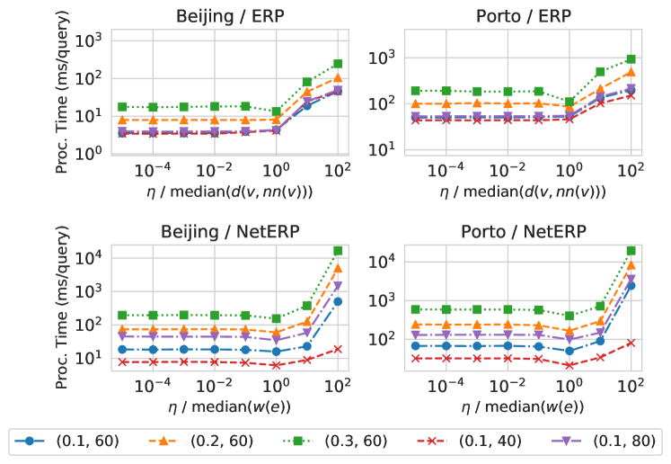
Figure 13: Varying $\eta$. Legend means $(\tau_{\text{ratio}},|Q|)$.

Appendix E Detailed Setup for Effectiveness Evaluation

We describe the detailed setup for travel time estimation in §6.2. To estimate the travel time of a given path $Q$, we find a set of similar subtrajectories to $Q$ in the database $\mathcal{T}=\{(P^{(id)},T^{(id)})\}$. Here we call this set training dataset. Given a matched similar subtrajectory $P_{i:j}^{(id)}$, we can define the corresponding travel time by $T_{j}^{(id)}\!\!-T_{i}^{(id)}$. We estimate the travel time by averaging the travel time of the similar subtrajectories. Note that, for a given $P^{(id)}$, there can be multiple subtrajectories that are similar to $Q$. In case of that, we chose the most similar subtrajectory. In case of ties, we chose the shortest subtrajectory (otherwise LORS and LCSS become significantly worse because they do not penalize the length of trajectories).

One issue here is how we evaluate the accuracy of the estimation, i.e., how to define the ground truth travel time. One option is using the average travel time of subtrajectories that exactly match to $Q$; however, this is problematic because travel time data used in this ground truth is also included in the training dataset. To avoid such data leakage, we employ cross-validation. Because the set of similar subtrajectories to $Q$ definitely includes the subtrajectories that exactly match $Q$, for each of these exact match subtrajectories $P^{(id)}_{i:j}$, we first exclude the travel time of $P^{(id)}_{i:j}$ from the training dataset, and then evaluate the accuracy of the average estimated travel time against the ground truth travel time. We repeat this process over all the subtrajectories that exactly match $Q$ and averaging the MSEs. The evaluation result is free from the data leakage discussed above.

To describe the above method formally, we first find the subtrajectories that exactly match $Q$. Suppose we have $N_{Q}$ exact match subtrajectories in the dataset. We compute the travel time for each of these exact match subtrajectoires, i.e., given a $P^{(id)}_{i:j}=Q$, we have $\omega:=T^{(id)}_{j}-T^{(id)}_{i}$. This is our ground truth. We denote the set of ground truths by $\Omega^{\text{exact}}:=\{\omega_{k}\mid k=1\ldots N_{Q}\}$.

By leave-one-out cross-validation, the MSE of exact match is defined by

$$MSE(\text{exact}):=\frac{1}{N_{Q}}\sum_{k=1}^{N_{Q}}(\omega_{k}-avg(\Omega_{-k}^{\text{exact}}))^{2},$$

where $\Omega_{-k}^{\text{exact}}$ is the set of ground truth data excluding the $k$-th travel time, i.e., $\Omega_{-k}^{\text{exact}}:=\Omega^{\text{exact}}\backslash\{\omega_{k}\}$.

Then, we conduct similarity search with a threshold $\tau_{\ratio}$. We define $\Omega^{\tau_{\text{ratio}}}:=\{T^{(id)}_{j}-T^{(id)}_{i}\mid\exists i,j\quad\text{s.t.\,}\textsf{wed}(Q,P_{i:j}^{(id)})\leq\tau_{\text{ratio}}\sum_{q\in Q}c(q)\}$. For each data trajectory $P^{(id)}$, we choose only one subtrajectory $P_{i:j}^{(id)}$ that best matches $Q$, i.e., the one with the smallest WED to $Q$ (we break tie by picking the one with the shortest length). By leave-one-out cross-validation, the MSE of similarity search is defined by

$$MSE(\tau):=\frac{1}{N_{Q}}\sum_{k=1}^{N_{Q}}(\omega_{k}-avg(\Omega_{-k}^{\tau_{\text{ratio}}}))^{2},$$

where $\Omega_{-k}^{\tau_{\text{ratio}}}$ is the set of estimated travel times excluding the $k$-the ground truth $\omega_{k}\in\Omega^{\text{exact}}$ (note that $\Omega^{\text{exact}}\subseteq\Omega^{\tau_{\text{ratio}}}$). Then RMSE is defined as $RMSE:=MSE(\tau)/MSE(\text{exact})$.

We repeat the above procedure for each query $Q$ and report the average RMSE.

Appendix F Discussion on LORS, LCRS, and SURS

We show the following fact: if two trajectories $x$ and $y$ are similar in terms of SURS, then they are also similar in terms of LCRS [64]. LORS [48] and LCRS have the following relation

$$\textsf{LCRS}(x,y)=\frac{\textsf{LORS}(x,y)}{w(x)+w(y)-\textsf{LORS}(x,y)}$$

In addition, LORS and SURS have the following relation

$$\textsf{SURS}(x,y)=w(x)+w(y)-2\cdot\textsf{LORS}(x,y).$$

Suppose that $x$ and $y$ are similar in terms of SURS. In this case, we have $w(x)+w(y)\simeq 2\cdot\textsf{LORS}(x,y)$. In addition, we also have $w(x)\simeq w(y)$ (because of the length filter). Therefore, we have $w(y)\simeq\textsf{LORS}(x,y)$ if $x$ and $y$ are similar in terms of SURS. This leads to the following approximation:

$$1-\textsf{LCRS}(x,y)\simeq\frac{\textsf{SURS}(x,y)}{w(x)}$$

If $\textsf{SURS}(x,y)\leq\tau_{ratio}\cdot w(x)$, then we approximately have $\textsf{LCRS}(x,y)\gtrapprox 1-\tau_{ratio}$. This is why SURS and LCRS behave similarly at small $\tau_{ratio}$.

References

- [1] I. Abraham, D. Delling, A. V. Goldberg, and R. F. Werneck. Hierarchical hub labelings for shortest paths. In ESA, pages 24–35, 2012.
- [2] T. Akiba, Y. Iwata, and Y. Yoshida. Fast exact shortest-path distance queries on large networks by pruned landmark labeling. In SIGMOD, pages 349–360, 2013.
- [3] I. Assent, R. Krieger, F. Afschari, and T. Seidl. The TS-tree: Efficient Time Series Search and Retrieval. In EDBT, pages 252–263, 2008.
- [4] T. Brinkhoff. A framework for generating network-based moving objects. GeoInformatica, 6(2):153–180, 2002.
- [5] T. Carnes and D. B. Shmoys. Primal-dual schema for capacitated covering problems. Mathematical Programming, 153(2):289–308, 2015.
- [6] L. Chen and R. Ng. On the marriage of lp-norms and edit distance. In VLDB, pages 792–803, 2004.
- [7] L. Chen, M. T. Özsu, and V. Oria. Robust and fast similarity search for moving object trajectories. In SIGMOD, pages 491–502, 2005.
- [8] Z. Chen, H. T. Shen, and X. Zhou. Discovering popular routes from trajectories. In ICDE, pages 900–911, 2011.
- [9] V. T. de Almeida and R. H. Güting. Indexing the trajectories of moving objects in networks. Geoinformatica, 9(1):33–60, 2005.
- [10] D. Deng, G. Li, and J. Feng. A pivotal prefix based filtering algorithm for string similarity search. In SIGMOD, pages 673–684, 2014.
- [11] M. R. Evans, D. Oliver, S. Shekhar, and F. Harvey. Fast and exact network trajectory similarity computation: a case-study on bicycle corridor planning. In UrbComp@KDD, pages 9:1–9:8, 2013.
- [12] J. Feng, J. Wang, and G. Li. Trie-join: a trie-based method for efficient string similarity joins. VLDB J., 21(4):437–461, 2012.
- [13] L. Gravano, P. G. Ipeirotis, H. V. Jagadish, N. Koudas, S. Muthukrishnan, and D. Srivastava. Approximate string joins in a database (almost) for free. In VLDB, pages 491–500, 2001.
- [14] J.-R. Hwang, H.-Y. Kang, and K.-J. Li. Searching for similar trajectories on road networks using spatio-temporal similarity. In ADBIS, pages 282–295, 2006.
- [15] H. Hyyrö and G. Navarro. A practical index for genome searching. In SPIRE, pages 341–349, 2003.
- [16] T. Idé and S. Kato. Travel-time prediction using gaussian process regression: A trajectory-based approach. In SDM, pages 1185–1196, 2009.
- [17] E. Keogh and C. A. Ratanamahatana. Exact indexing of dynamic time warping. Knowledge and Information Systems, 7(3):358–386, 2005.
- [18] S. Koide, K. Kawano, and T. Kutsuna. Neural edit operations for biological sequences. In Advances in Neural Information Processing Systems 31, pages 4965–4975, 2018.
- [19] S. Koide, Y. Tadokoro, C. Xiao, and Y. Ishikawa. CiNCT: Compression and retrieval for massive vehicular trajectories via relative movement labeling. In ICDE, pages 1097–1108, 2018.
- [20] S. Koide, Y. Tadokoro, T. Yoshimura, C. Xiao, and Y. Ishikawa. Enhanced indexing and querying of trajectories in road networks via string algorithms. ACM Trans. Spatial Algorithms Syst., 4(1):3:1–3:41, 2018.
- [21] B. Krogh, C. S. Jensen, and K. Torp. Efficient in-memory indexing of network-constrained trajectories. In GIS, pages 17:1–17:10, 2016.
- [22] B. Krogh, N. Pelekis, Y. Theodoridis, and K. Torp. Path-based queries on trajectory data. In GIS, pages 341–350, 2014.
- [23] C. Li, B. Wang, and X. Yang. VGRAM: improving performance of approximate queries on string collections using variable-length grams. In VLDB, pages 303–314, 2007.
- [24] G. Li, D. Deng, and J. Feng. A partition-based method for string similarity joins with edit-distance constraints. ACM Trans. Database Syst., 38(2):9:1–9:33, 2013.
- [25] H. Li and R. Durbin. Fast and accurate short read alignment with burrows–wheeler transform. Bioinformatics, 25(14):1754–1760, 2009.
- [26] H. Li and R. Durbin. Fast and accurate long-read alignment with Burrows-Wheeler transform. Bioinformatics, 26(5):589–595, 2010.
- [27] X. Li, K. Zhao, G. Cong, C. S. Jensen, and W. Wei. Deep representation learning for trajectory similarity computation. In ICDE, pages 617–628, 2018.
- [28] W. Luo, H. Tan, L. Chen, and L. M. Ni. Finding time period-based most frequent path in big trajectory data. In SIGMOD, pages 713–724, 2013.
- [29] C. D. Manning, P. Raghavan, and H. Schütze. Introduction to Information Retrieval. Cambridge University Press, 2008.
- [30] M. F. Mokbel, T. M. Ghanem, and W. G. Aref. Spatio-Temporal Access Methods. IEEE Data Eng. Bull., 26(2):40–49, 2003.
- [31] L. Moreira-Matias, J. Gama, M. Ferreira, J. Mendes-Moreira, and L. Damas. Predicting taxi-passenger demand using streaming data. IEEE Trans. Intelligent Transportation Systems, 14(3):1393–1402, 2013.
- [32] M. D. Morse and J. M. Patel. An efficient and accurate method for evaluating time series similarity. In SIGMOD, pages 569–580, 2007.
- [33] S. Needleman and C. Wunsch. A general method applicable to the search for similarities in the amino acid sequence of two proteins. Journal of Molecular Biology, 48(3):443–453, 3 1970.
- [34] P. Newson and J. Krumm. Hidden Markov map matching through noise and sparseness. In GIS, pages 336–343, 2009.
- [35] L.-V. Nguyen-Dinh, W. G. Aref, and M. F. Mokbel. Spatio-Temporal Access Methods : Part 2 (2003 – 2010). IEEE Data Eng. Bull., 33(2):46–55, 2010.
- [36] J. Qin, W. Wang, C. Xiao, Y. Lu, X. Lin, and H. Wang. Asymmetric signature schemes for efficient exact edit similarity query processing. ACM Trans. Database Syst., 38(3):16:1–16:44, 2013.
- [37] S. Ranu, D. P, A. D. Telang, P. Deshpande, and S. Raghavan. Indexing and matching trajectories under inconsistent sampling rates. In ICDE, pages 999–1010, 2015.
- [38] Y. Sakurai, C. Faloutsos, and M. Yamamuro. Stream monitoring under the time warping distance. In ICDE, pages 1046–1055, 2007.
- [39] S. Shang, L. Chen, Z. Wei, C. S. Jensen, K. Zheng, and P. Kalnis. Trajectory Similarity Join in Spatial Networks. Proc. VLDB Endow., 10(11):1178–1189, 2017.
- [40] S. Shang, R. Ding, K. Zheng, C. S. Jensen, P. Kalnis, and X. Zhou. Personalized trajectory matching in spatial networks. VLDB J., 23(3):449–468, 2014.
- [41] Z. Shang, G. Li, and Z. Bao. DITA: Distributed In-Memory Trajectory Analytics. In SIGMOD, pages 725–740, 2018.
- [42] C.-B. Shim and J.-W. Chang. Similar sub-trajectory retrieval for moving objects in spatio-temporal databases. In ADBIS, pages 308–322, 2003.
- [43] T. F. Smith and M. S. Waterman. Identification of common molecular subsequences. Journal of Molecular Biology, 147(1):195–197, 1981.
- [44] R. Song, W. Sun, B. Zheng, and Y. Zheng. PRESS: A novel framework of trajectory compression in road networks. Proc. VLDB Endow., 7(9):661–672, 2014.
- [45] H. Su, S. Liu, B. Zheng, X. Zhou, and K. Zheng. A survey of trajectory distance measures and performance evaluation. VLDB J., 29(1):3–32, 2020.
- [46] E. Tiakas, A. Papadopoulos, A. Nanopoulos, Y. Manolopoulos, D. Stojanovic, and S. Djordjevic-Kajan. Searching for similar trajectories in spatial networks. Journal of Systems and Software, 82(5):772 – 788, 2009.
- [47] M. Vlachos, D. Gunopulos, and G. Kollios. Discovering similar multidimensional trajectories. In ICDE, pages 673–684, 2002.
- [48] S. Wang, Z. Bao, J. S. Culpepper, Z. Xie, Q. Liu, and X. Qin. Torch: A search engine for trajectory data. In SIGIR, pages 535–544, 2018.
- [49] W. Wang, J. Qin, C. Xiao, X. Lin, and H. T. Shen. Vchunkjoin: An efficient algorithm for edit similarity joins. IEEE Trans. Knowl. Data Eng., 25(8):1916–1929, 2013.
- [50] W. Wang, C. Xiao, X. Lin, and C. Zhang. Efficient approximate entity extraction with edit distance constraints. In SIGMOD, pages 759–770, 2009.
- [51] Y. Wang, Y. Zheng, and Y. Xue. Travel time estimation of a path using sparse trajectories. In KDD, pages 25–34, 2014.
- [52] R. Waury, J. Hu, B. Yang, and C. S. Jensen. Assessing the accuracy benefits of on-the-fly trajectory selection in fine-grained travel-time estimation. In MDM, pages 240–245, 2017.
- [53] R. Waury, C. S. Jensen, S. Koide, Y. Ishikawa, and C. Xiao. Indexing trajectories for travel-time histogram retrieval. In EDBT, pages 157–168, 2019.
- [54] H. Wei, J. X. Yu, and C. Lu. String similarity search: A hash-based approach. IEEE Trans. Knowl. Data Eng., 30(1):170–184, 2018.
- [55] J. I. Won, S. W. Kim, J. H. Baek, and J. Lee. Trajectory clustering in road network environment. In CIDM, pages 299–305, 2009.
- [56] Y. Xia, G. Y. Wang, X. Zhang, G. B. Kim, and H. Y. Bae. Spatio-temporal Similarity Measure for Network Constrained Trajectory Data. Int. J. Comput. Intell. Syst., 4(5):1070–1079, 2011.
- [57] C. Xiao, W. Wang, and X. Lin. Ed-Join : An Efficient Algorithm for Similarity Joins With Edit Distance Constraints. Proc. VLDB Endow., 1(1):933–944, 2008.
- [58] D. Xie, F. Li, and J. M. Phillips. Distributed trajectory similarity search. Proc. VLDB Endow., 10(11):1478–1489, 2017.
- [59] L. Yang, Y. Wang, Q. Bai, and S. Han. Urban Form and Travel Patterns by Commuters: Comparative Case Study of Wuhan and Xi’an, China. Journal of urban planning and development, 144(1):05017014, 2018.
- [60] X. Yang, H. Liu, and B. Wang. ALAE: Accelerating Local Alignment with Affine Gap Exactly in Biosequence Databases. Proc. VLDB Endow., 5(11):1507–1518, 2012.
- [61] X. Yang, B. Wang, and C. Li. Cost-based variable-length-gram selection for string collections to support approximate queries efficiently. In SIGMOD, pages 353–364, 2008.
- [62] D. Yao, G. Cong, C. Zhang, and J. Bi. Computing trajectory similarity in linear time: A generic seed-guided neural metric learning approach. In ICDE, pages 1358–1369, 2019.
- [63] B. Yi, H. V. Jagadish, and C. Faloutsos. Efficient retrieval of similar time sequences under time warping. In ICDE, pages 201–208, 1998.
- [64] H. Yuan and G. Li. Distributed in-memory trajectory similarity search and join on road network. In ICDE, pages 1262–1273, 2019.
- [65] J. Yuan, Y. Zheng, C. Zhang, W. Xie, X. Xie, G. Sun, and Y. Huang. T-drive: driving directions based on taxi trajectories. In GIS, pages 99–108, 2010.
- [66] Y. Zheng and X. Zhou. Computing with Spatial Trajectories. Springer, 2011.