Tree Annotations in LiDAR Data Using Point Densities and Convolutional Neural Networks

Abstract

LiDAR provides highly accurate 3D point clouds. However, data needs to be manually labelled in order to provide subsequent useful information. Manual annotation of such data is time consuming, tedious and error prone, and hence in this paper we present three automatic methods for annotating trees in LiDAR data. The first method requires high density point clouds and uses certain LiDAR data attributes for the purpose of tree identification, achieving almost 90% accuracy. The second method uses a voxel-based 3D Convolutional Neural Network on low density LiDAR datasets and is able to identify most large trees accurately but struggles with smaller ones due to the voxelisation process. The third method is a scaled version of the PointNet++ method and works directly on outdoor point clouds and achieves an $F_{score}$ of 82.1% on the ISPRS benchmark dataset, comparable to the state-of-the-art methods but with increased efficiency.

I Introduction

Trees are essential components of both natural and urban environments; not only are they aesthetically pleasing, but also they help regulate ecological balance in the landscapes and maintain air quality by reducing particulate matter in the environment [1]. Urban forest inventories are important assets for planning and management of urban environments since many applications, such as mitigation of noise [2] and creation of 3D city models [3], make use of such data sources. Traditional tree inventories are done manually and the process is extremely time consuming [4].

Along with terrestrial LiDAR and Unmanned Aerial Vehicle photogrammetry, airborne LiDAR systems are advanced methods used for 3D data acquisition of urban environments [5]. LiDAR utilises laser pulses to measure distances to sufficiently opaque surfaces and objects and enable the study of 3D structure and properties of a given environment.

There is a large body of work on tree identification using LiDAR data, but most of it focuses on identifying trees in forested environments, with little emphasis given to urban environments. Most of these methods are derivatives of the canopy height model (CHM) [6, 7, 8, 9, 10].

The existing methods for tree identification in forests are not directly applicable to urban areas because the statistics of the two environments are very different. The assumption of homogeneous and highly dense collections of trees in forests does not apply in the urban environments. Urban areas are extremely complex and heterogeneous and include isolated trees and groups of trees, often of different species, ages and shapes. The presence of other vertical objects and features such as buildings and street lamps, which typically do not exist in forested environments, makes the problem even more complex.

There has been some pioneering work in urban tree detection based on machine learning. A combination of aerial images and LiDAR data has been used for segmentation followed by classification with support vector machines (SVM) [11]. This work has been extended to use features derived from depth images of LiDAR data with a random forest classifier and achieved precision recall scores of 95% in identifying trees in the depth images [12]. However, the accuracy degraded to below 75% when the training and testing were done on separate datasets. Another method [13] used a cascade of binary classifiers to progressively identify water, ground, roofs and trees by conducting 3D shape analysis followed by region growth. Segmentation of foreground and background, followed by classification of object-like clusters using different methods such as k-nearest neighbours, SVMs and random forests was used to locate different 3D objects in an urban environment [14]. Decision trees and artificial neural networks using segmented features derived from full waveform attributes have also been used in classification [15].

Identification of trees in urban environments with heuristics-based methods has also been studied. Liu et al. [16] proposed a method for extracting tree crowns by filtering out ground points and using a spoke wheel method to get tree edges. The method was able to detect over 85% of trees from the test dataset with 95% accuracy. However, it only focused on extracting tree crowns and did not take tree trunks into account and was unsuited for urban forest inventory applications. A voxel-based method was used to extract individual trees from mobile laser scanning data but it was not suitable for use with airborne LiDAR scans  [17]. A combination of LiDAR and hyperspectral data to detect treetops and a region growing algorithm for segmentation has also been developed for urban forest inventory purposes [18].

Recent work based on deep learning has shown promising results in identifying objects in LiDAR scans of urban environments. Yousefhussien et al. [19] used a 1D convolutional neural network (CNN) in conjunction with LiDAR data and spectral information to generate point-wise semantic labels for unordered points and achieved a mean $F_{score}$ of 63.32% on the ISPRS Benchmark [20]. Multiple CNNs have been used to learn per-point features of different data attributes (height, intensity and roughness) from multi-scale images for classification [21]. However, this method was computationally expensive as it generated multiple contextual images per point in the dataset and classified each point individually. Another method along similar lines used a CNN in conjunction with 2D images derived from the point clouds for point-based classification [22]. The method was also extremely computationally expensive and relied on hand-engineered feature images, contrary to the popular use of CNNs for extracting features implicitly. The method also required a cleanly labelled training set with all categories for multi-category classification.

In this paper, we propose three methods for automatic tree identification in LiDAR data in urban environments. All three methods work on point cloud data and the third method has been adapted to combine spectral data with the point locations.

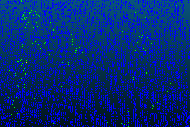
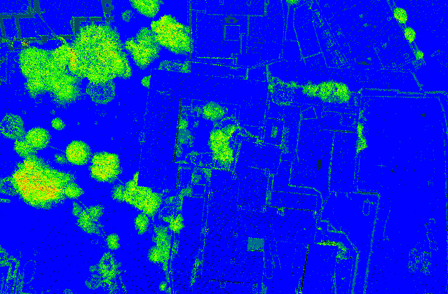
The first method, termed as MultiReturn, is based on our earlier work [23] and uses traditional handcrafted features as well as inherent data characteristics of LiDAR data. It works well on datasets that have point cloud density $>$$20\text{\,}\mathrm{points}\text{\,}{\mathrm{m}}^{-2}$ as these datasets contain the number of returns characteristic that allows the method to identify trees. However, it is unable to deal with point clouds with lower resolutions, since they do not exhibit the same characteristic, as illustrated in Figure 1.

(a) Low Density Point Cloud.

(b) High Density Point Cloud.

Figure 1: Point clouds with red showing high number of returns decreasing to blue representing single return. Left: Low density point cloud hence very few points with high number of returns per point. Right: High density point cloud hence more dense collections of points with a high number or returns per point.

The second method, termed as TreeNet, is based on a 3D CNN and works on voxelised datasets. It can be trained using the results of the first method and is able to identify large trees with good accuracy. However, it struggles to identify small trees due to the limited resolution of voxels.

The third method, sPointNet++, is based on PointNet++ [24], a state-of-the-art method for 3D shape classification and indoor point cloud segmentation. We scale it to include spectral information for dealing with outdoor aerial datasets, which are much noisier than indoor data. It works directly with point clouds and is able to identify smaller trees well. However, it requires a large amount of cleanly labelled training data, which can be troublesome to obtain. We adapt the training loss to deal with unbalanced class distributions, allowing the network to train a binary classifier with very few positive points (tree category) relative to large negative points (non-tree points).

II Methods

II-A MultiReturn: Tree Annotation with Number of Returns

The first method, MultiReturn [23], which can be reformulated in Algorithm 1, is based on four distinct steps:

• Ground filtering

• Voxelising non-ground point cloud data

• Isolating tree-like regions using the information gained from the number of returns

• Post-processing to remove false positives.

Algorithm 1 Tree Annotation with Number of Returns

Input: Point Cloud pcd       Output: Tree data trees

1:$filtered\_cloud$ = []

2:$filtered\_vox$ = []

3:$trees$ = []

4:$gnd\_points$ = PMF($pcd$)

5:for $point$ in $pcd$ do

6:     if $point$ not in $gnd\_points$ then

7:         $filtered\_cloud$.append($point$)

8:     end if

9:end for

10:$vox\_cloud$ = Voxelise($filtered\_cloud$)

11:for $vox$ in $vox\_cloud$ do

12:     if $vox$.$no\_of\_returns$ $>$ $ret\_thresh$ then

13:         $filtered\_vox$.append($vox$)

14:     end if

15:end for

16:$vox\_regions$ = ConnectedComponents($filtered\_vox$)

17:for $region$ in $vox\_regions$ do

18:     if $region$.size $>$ $comp\_threshold$ then

19:         if $region.x$/$region.y$ $\geq$ 2 or $region.y$/$region.x$ $\geq$ 2 then

20:              continue;

21:         else

22:              $trees$.append($region$)

23:         end if

24:     end if

25:end for

(a) Original Point Cloud.

(b) Result after cleaning for ground and noise.

Figure 2: Ground filtering process with points coloured according to height.

In order to identify and filter the ground points, we use a progressive morphological filter (PMF) [25]. It uses morphological erosion and dilation operations in conjunction with windows of progressively increasing size to identify non-ground points. This is followed by statistical outlier removal to remove noisy points that are below the ground level and a filtered result can be seen in Figure 2(b).

The publicly available Point Data Abstraction Library (PDAL) [26] was used for this filtering process. The filters.pmf package with a window size of $40\text{\,}\mathrm{m}$ and maximum distance of $3.5\text{\,}\mathrm{m}$ was used for ground filtering and the filters.outlier function was used for statistical outlier removal with the default values given in the package.

The point cloud is converted into a volumetric occupancy grid in order to make the data easier to deal with, because it reduces dimensionality. A fixed size 3D grid is overlaid on the point cloud and the occupancy of each cell depends on the presence of points within the cell, i.e. the cell is unoccupied if there are no points in the cell’s volume and vice versa. In this case, each volumetric element, voxel, represents a grid cell in the subsampled point cloud.

We use VOLA [27] to encode the voxel representation in a sparse format. VOLA is a hierarchical 3D data structure that draws inspiration from octree based data structures. But unlike standard octrees it only encodes occupied voxels in a “1-bit per voxel” format, and hence is extremely memory efficient. In this case we use a “2-bit per voxel” format to encode additional information per voxel such as colour, number of returns and intensity value.

LiDAR datasets are acquired by pulsing laser light and measuring the time that the pulse takes to reflect from sufficiently opaque surfaces to calculate the distance to said surface. A single pulse can reflect completely in one collision with a surface or can reflect multiple times when it encounters edges that reflect the light partially. In high point density datasets, trees typically have multiple returns as pulses are partially reflected from the edges of leaves. Leaf-off trees also have similar characteristics since they still have a number of branches and twigs giving similar patterns of returns. Other features that can have a high number of returns are building edges and window ledges. However, returns in these latter cases are more scattered than that in the case of trees, where a large number of high returns are closely packed as can be seen in Figure 1(b).

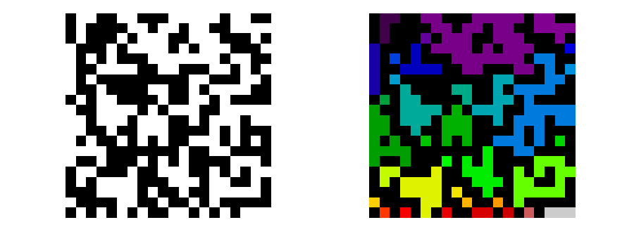
We use this insight to isolate tree regions by identifying voxels with multiple returns (empirically identified as more than 3 returns per voxel) and then performing a connected component analysis on these voxels. A connected component is a subgraph in an undirected graph where any two vertices are connected to each other by paths. In this case, regions of dense voxels with at least one common edge are marked as connected components. An example of 2D connected component labelling has been shown in Figure 3, this is easily extendable to 3D by replacing the 2D cells with 3D voxels.

Figure 3: Connected Components in 2D. Left: White indicates occupied cells, Black unoccupied; Right: Each region identified as a connected block is represented by a different colour.

Regions of high returns with a minimum number of connected components, $ncc$, are then identified as tree regions, while any regions with fewer components than the threshold value are discarded as noise from buildings, corners, etc.

$$f_{x}=\left\{\begin{matrix}1,&ncc\geq threshold\\ 0&ncc<threshold\end{matrix}\right\}$$ (1)

The tree regions isolated by connected components are typically tree canopies as trunk voxels with a high number of returns are typically sparse and not well connected. In order to find tree trunks, the maximum and minimum $x$ and $y$ coordinates of each region are identified, along with the maximum $z$ coordinate. These coordinates are then used to place a 3D bounding box in the original data near the ground level in order to capture the trunk information. The width to length ratio of the bounding box is constrained so that they are approximately equal. Any regions not matching these constraints are discarded as a false positive. Upon manual inspection of the results and statistical analysis, it could be seen that although this resulted in removing some trees, all the walls covered with ivy are removed.

II-B TreeNet: 3D CNN for Tree Segmentation

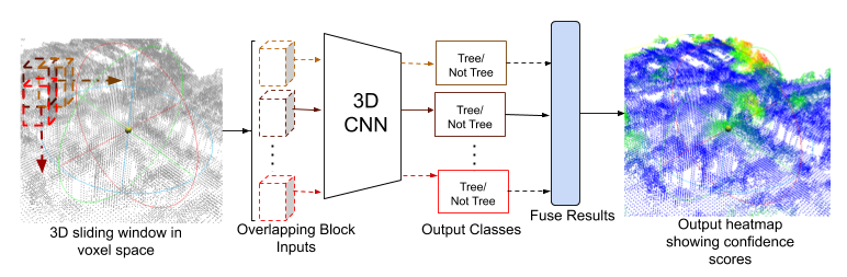
Inspired by the recent successes of CNNs in image classification, we propose TreeNet, a deep learning approach based on 3D voxels to deal with low density point clouds. A 3D CNN is designed for binary classification of 3D voxel spaces for presence or absence of trees. The output labels from sliding voxel windows of the network are fused to provide a per voxel confidence score. The system architecture is shown in Figure 4.

Figure 4: Block Diagram for TreeNet Segmentation. Left: LiDAR point cloud subdivided into overlapping blocks. Middle: Each block processed individually by CNN with binary output. Right: Results fused to provide a confidence score per point.

TABLE I: 3D CNN Architecture Details

Layer Type	Details
Conv3D	5x5x5 filter size
	32 filters
	stride = 2
Dropout3D	p = 0.2
Conv3D	3x3x3 filter size
	32 filters
	stride = 1
MaxPool3D	2x2x2 window size
Dropout3D	p = 0.3
FC	128 features
Dropout3D	p = 0.4
FC	2

3D CNNs are extensions of the standard 2D CNNs and are used here for two main reasons: their ability to learn local spatial features in 3D space instead of relying on traditional handcrafted features, and their ability to encode more complex relationships of hierarchical features with combinations of multiple layers. The input to the network is a multi-channel 3D volume in $\mathbb{R}^{w\times h\times d\times c_{i}}$ where $w$, $h$ and $d$ are the spatial dimensions of the input volume and $c_{i}$ is the number of input channels.

The data is processed through a series of 3D convolutional layers. Each layer, $l$, consists of $c_{l}$ filters where each 3D filter, $K^{l}$, is convolved with the input voxel (for the first layer) or the output of the previous layer, $O^{l-1}$ (for subsequent layers). The output from layer $l$ is given by $O^{l}$ and is calculated using Equation 2.

$$O^{l}_{n}=\sum_{m=0}^{c_{l-1}}O_{m}^{l-1}*K^{l}_{m,n}\textrm{ where }n=1,2,3,...,c_{l}$$ (2)

The output activations from the convolutional layers are passed through a leaky Rectified Linear Unit (ReLU) [28, 29] with a slope of 0.1. A 3D Max Pooling layer is used for downsampling the data, hence reducing the dimensionality and making the computation more efficient. Dropout [30] layers are used for preventing overfitting.

The final two layers in the network are fully connected (FC) layers to learn weighted combinations of the extracted feature maps. The cross entropy loss is used for training the network.

The details of the CNN architecture are listed in Table I where the input is a 20x20x100 voxel volume. Variable p in the dropout layer indicates the probability of the elements being replaced with zeroes.

The output from the final FC layer is a binary class label indicating whether the input box area contains a tree or not. A sliding window with overlap in both horizontal dimensions is used over the dataset for classification. In order to convert this to a per-voxel result, the output classification is mapped back to the input voxels. With the overlapping windows used, each voxel has multiple output values. A voting scheme is used to get the final result. If over 40% of these outputs are positive, the voxel is identified as belonging to a tree. The 40% threshold was chosen empirically based on the experimental results.

II-C Scaling Pointnet++

PointNet++ [24] is the state-of-the-art method in point cloud segmentation of indoor environments. Herein, we provide a scaled version called sPointNet++ to deal with aerial urban LiDAR scans and to work directly with unordered point sets instead of the regularly spaced voxel grids as in the previous methods. Aerial laser scans, in comparison to indoor scenes, tend to be noisier and have more terrain and point density variations across scenes. In order to deal with these issues, we augment the model with the use of spectral information in addition to point cloud data.

The 2D spectral aerial image containing IR-R-G (Infrared-Red-Green) values is fused with the point cloud. Bilinear interpolation in the image plane is used to assign IR-R-G information to each point in the dataset. The outline of the model used is given in Table II and the description of the layers is as follows:

Sampling and Grouping Layer: uses furthest point sampling (FPS) [31], which is an iterative sampling process that picks the next sample from the least known region in the sampling domain, to identify a subset of $N_{l}$ input points as centroids. These centroids are used to identify points within a local region around the centroids using a ball query of radius $r$ and the output from this layer are point sets of size $N_{l}\times K\times\left(d+C\right)$, where $K$ is the number of points in a local region around each centroid, $d$ is the dimensionality of the point coordinates, and $C$ is the dimensionality of point information such as spectral data. This allows for uniform coverage of point clouds that have non-uniform point density, common in aerial laser scans due to varying scanning patterns. In order to learn hierarchical features, a number of these layers are stacked in a series with varying radius for the neighbourhood ball query to encode features at different resolutions.

PointNet layer: the output from the sampling and grouping layer is processed with a PointNet layer [32] which learns an abstracted local feature per centroid. The output data has size $N_{l}\times C^{\prime}$, where $C^{\prime}$ gives the abstracted features per centroid. The PointNet layer is a set of $n$ 1x1 convolution layers with the numbers of filters in each 1x1 layer given by $[l_{1},..,l_{n}]$.

Feature Set Propagation: in order to provide a per point label for semantic segmentation, the feature labels are propagated from the subsampled points to the original points with distance-based interpolation and skip links as shown in Figure 5. Each point could be used as a centroid to get per point labels but only at the cost of high computation. The interpolation is done with a less computationally intensive method explained below.

Figure 5: sPointNet++ Architecture.

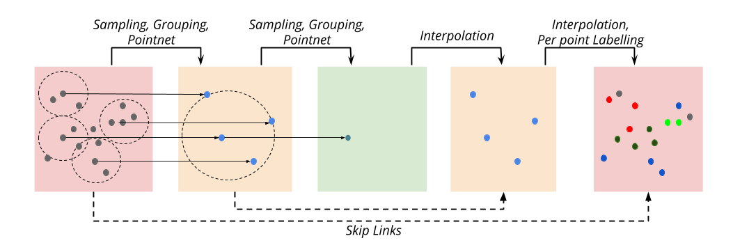
The feature propagation layers are essentially a mirror of the feature sampling layers. In set sampling, the number of input points and output points is $N_{l-1}$ and $N_{l}$ respectively, where $N_{l}<N_{l-1}$, whereas in feature propagation the input is $N_{l}$ and the output is $N_{l-1}$. This is done by interpolating the $N_{l}$ values to $N_{l-1}$ using an inverse-distance weighted average of $k$ nearest neighbours, with $k$ being set to 3 and the weight being given by the inverse of the Euclidean distance between the points. These are concatenated with skip link features from the corresponding sampling layer followed by $m$ 1x1 convolution layers, with the width of each 1x1 layer given by $[l_{1},..l_{m}]$ in Table II. The final layers are a number of FC layers (implemented as 1x1 convolutions to allow for variable size inputs) with ReLU activations. The output is a per-class confidence score for every input point.

TABLE II: sPointNet++ Architecture

Layer	Details
Sampling and Grouping	$N_{1}$=1024, r=1.5 , K=32 ,d=3, C=3)
PointNet	[32,32,64]
Sampling and Grouping	$N_{1}$=256, r=3 , K=32)
PointNet	[64,64,128]
Sampling and Grouping	$N_{1}$=64, r= 6 , K=32)
PointNet	[128,128,256]
Sampling and Grouping	$N_{1}$=16, r=12 , K=32)
PointNet	[256, 256, 512]
Feature Set Propagation	[256,256]
Feature Set Propagation	[256,256]
Feature Set Propagation	[256,128]
Feature Set Propagation	[128,128,128]
FC	[128]
FC	[2]

Since the class distribution is highly unbalanced with only about 15% of the points in the training set being positive samples, we use a weighted cross entropy loss to train the network. The output classes are weighted inversely to the occurrence of a specific label in the training set, so that classes which occur less frequently are weighted more when calculating the output loss. This discourages the network from always labelling the few positive samples as negative since this is a local minima in the unweighted loss space that the network would converge to. The loss function used is:

$$L=-w_{c}\left[log\frac{e^{o_{c}}}{\sum_{j=1}^{C}e^{o_{j}}}\right]$$ (3)

which can be rewritten as:

$$L=w_{c}\left[-o_{c}+log\sum_{j=1}^{C}e^{o_{j}}\right]$$ (4)

where $L$ is the loss per sample, $o_{c}$ is the output value for the target class $c$ and $w_{c}$ is the weight of the target class which is calculated over all classes $C$ as:

$$w_{c}=\frac{\max\limits_{i\in\{1,..,C\}}\left(S_{i}\right)}{S_{c}}$$ (5)

where $S_{i}$ is the number of samples of class $i$.

In order to train the network, random blocks of different sizes were sampled from the point cloud as training samples, with 4096 sampling points per block. The sampling ball radius was varied between $0.3\text{\,}\mathrm{m}$ and $2\text{\,}\mathrm{m}$, while the block width varied between $10\text{\,}\mathrm{m}$ to $20\text{\,}\mathrm{m}$ for different data types. The block size informs the encoding of the global features while the sampling ball radius affects the local features learnt by the network. However, due to the inherent multiscale feature encoding in the network, it was seen that the results remained mostly consistent across different sizes and hence the results reported were obtained with the input sampling radius of $1.5\text{\,}\mathrm{m}$ and block size of $15\text{\,}\mathrm{m}$.

III Experimental Setup

III-A Datasets

The following datasets were used for evaluating the proposed methods:

• 2015 Aerial Laser and Photogrammetry Survey of Dublin City [33]

• Montreal 2015 Aerien Survey [34]

• ISPRS Urban Classification Benchmark dataset [20]

The MultiReturn method was tested on the Dublin city dataset. This dataset, captured at an altitude of $300\text{\,}\mathrm{m}$ using a TopEye system S/N 443, consists of over 600 million points with an average point density of $348.43\text{\,}\mathrm{points}\text{\,}{\mathrm{m}}^{-2}$. It covered an area of $2\text{\,}{\mathrm{km}}^{2}$ in Dublin city centre. Following the original tile dimensions of $$100\text{\,}\mathrm{m}$\times$100\text{\,}\mathrm{m}$$ of the dataset, each tile was converted into a voxel grid of dimensionality $256\times 256\times 256$ hence limiting the resolution of the voxel grid to $\approx$0.39\text{\,}\mathrm{m}$\times$0.39\text{\,}\mathrm{m}$\times$0.39\text{\,}\mathrm{m}$$ per voxel.

The results from the MultiReturn algorithm were validated using the labels from Ningal [35] containing tree annotations around some of the major streets in Dublin from 2008. In order to get more up to date results, the region north of the Liffey river was manually annotated for trees using satellite imagery from Google Earth in 2015.

The Montreal dataset is an aerial survey of the territory of Montreal city. It covers an area of over $775\text{\,}{\mathrm{km}}^{2}$, large enough for use in CNN training. The MultiReturn method was applied on this dataset for labelling trees which were used as positive samples for training TreeNet. An equal number of negative samples were sampled randomly from this dataset.

The ISPRS dataset was acquired using the Leica ALS50 system and has a point density of approximately $8\text{\,}\mathrm{points}\text{\,}{\mathrm{m}}^{-2}$. It has been provided by the German Society for Photogrammetry, Remote Sensing and Geoinformation (DGPF) over Vaihingen in Germany [36]. It has per point class labels and separate training and test sets, which were used to train sPointNet++ and test the segmentation results.

In all cases for training the CNNs, 10% of the training dataset was held aside as a validation set.

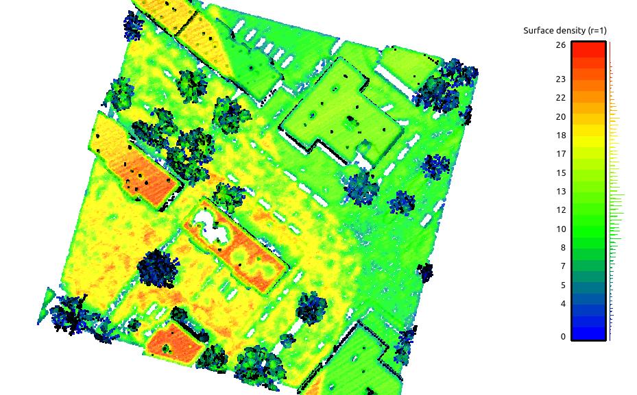
Note on Point Density: most LiDAR datasets report average point density as a statistic of the dataset. However, this statistic is not always well defined and can vary across datasets due to intentional or unintentional bias [37]. Furthermore, a small LiDAR dataset can have a large variance in its point density and due to the law of large numbers, the variance decreases as the dataset becomes larger (millions or billions of points).

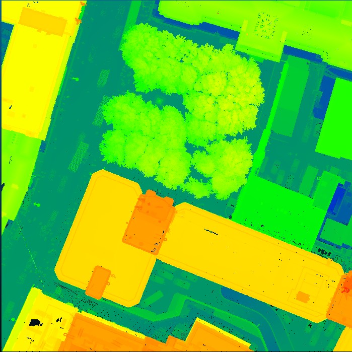
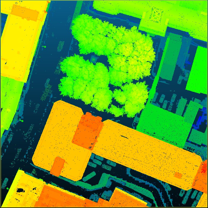
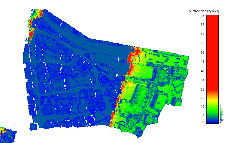
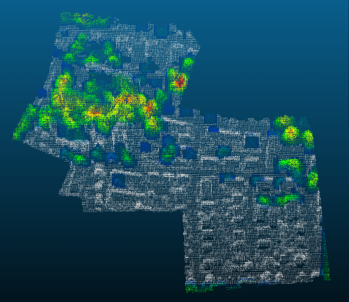
Point density also varies within a dataset and there is no standard metric to calculate point density across datasets. Some may report theoretical density values whereas others calculate them from on the dataset. Hence, even though both the Montreal and the ISPRS datasets reportedly have a point density of $8\text{\,}\mathrm{points}\text{\,}{\mathrm{m}}^{-2}$, their actual point statistics are quite different as can be seen in Figure 6 where the surface point densities of the two datasets are plotted as a heatmap. The figure shows that the point density varies across the two datasets and within the same datasets, especially in the case of Vaihingen, which is extremely sparse in parts of the scan. Due to this disparity, only the Montreal dataset could be used in the first method for tree annotation.

(a) Vaihingen Point Density.

(b) Montreal Point Density.

Figure 6: Surface Density plotted as heatmap for different LiDAR datasets. The density range was different between the two datasets and hence the heatmap colour scale was saturated at the same value to enable a valid visual comparison.

III-B Evaluation Metrics

The metrics presented in the ISPRS 3D labelling contest were used in the experiments for the purpose of evaluation. These metrics are precision or correctness, recall or completeness and $F_{score}$, defined as follows:

$$\begin{split}r=\frac{TP}{TP+FN}\\ p=\frac{TP}{TP+FP}\\ F_{score}=2\times\frac{r\times p}{r+p}\end{split}$$ (6)

where $TP$ is the number of true positives, $FN$ is the number of false negatives, $FP$ is the number of false positives and $F_{score}$ is the overall accuracy.

For the purpose of MultiReturn, the results were based on the detection of individual trees where a tree was assumed to be correctly identified if the predicted stem location was within $1.5\text{\,}\mathrm{m}$ of the actual stem location. The results for TreeNet and sPointNet++ were evaluated per voxel and per point, respectively.

III-C Tools

The initial noise and ground filtering of the LiDAR dataset was done using the publicly available Point Data Abstraction Library (PDAL) [26]. CloudCompare [38] was used for the point cloud visualisations. PyTorch [39] and TensorFlow [40] were used for building and training the CNNs.

III-D Training Details

TreeNet was trained using stochastic gradient descent with an initial learning rate of 0.01, momentum of 0.9 and exponential weight decay at a rate of 0.001. It was trained for up to 50 epochs.

sPointNet++ was trained using the Adam optimiser [41] with an initial learning rate of 0.001 and exponential decay at a rate of 0.7. It was trained till the validation loss converged up to a maximum of 200 epochs.

IV Results And Discussion

IV-A Tree Annotation with MultiReturn

Locations of trees in the Dublin dataset labelled by the MultiReturn method are shown in Figure 7 along with two sets of manually labelled locations as explained in Section III-A. The performances are summarised in Table III.

The results from Experiment 1 seem to suggest that the accuracy of this labelling method is not very high with an $F_{score}$ of 0.66. However, since the original annotations for this experiment were from 2008, it was discovered that they were out-of-date since the urban landscape of the city had changed significantly between the dates of the annotations and the acquisition of the LiDAR dataset for the development of the city tram network.

TABLE III: Summary of Results using MultiReturn

Experiment	Trees	TP	FP	FN	$p$	$r$	Fscore
1	313	178	45	135	0.57	0.8	0.66
2	535	469	56	66	0.88	0.89	0.88

(a) Experiment 1: Results compared to labels from manual study done in 2008.

(b) Experiment 2: Results compared to labels from Google Earth Imagery in 2015.

Figure 7: Map of survey area with tree locations shown in yellow and the outputs of our MultiReturn [23] labelling algorithm shown in red.

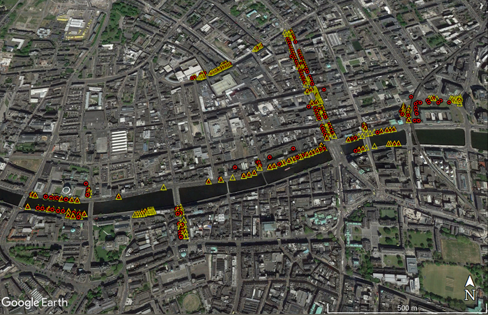
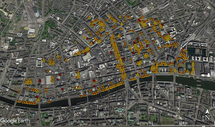
Experiment 2 used annotations from the aerial imagery of 2015 acquired from the Google Earth for a fair comparison. The proposed method gave good results with an $F_{score}$ of 0.89. It was especially good in identifying isolated trees with non-converging canopies. However, it did not perform well in areas such as parks where the tree canopies were merged as it could not identify such trees individually. Some merged canopies were removed by the tree width and height constraints, which were required for the removal of ivy-covered walls.

IV-B TreeNet for Segmentation

The ISPRS test dataset was voxelised to a resolution of $\approx$0.39\text{\,}\mathrm{m}$\times$0.39\text{\,}\mathrm{m}$\times$0.39\text{\,}\mathrm{m}$$ per voxel to match the resolution of the Dublin dataset. From the statistics of the training dataset, it was observed that most of the trees would have spatial dimensions of less than $8\text{\,}\mathrm{m}$ $\times$ $8\text{\,}\mathrm{m}$ with height varying upto $25\text{\,}\mathrm{m}$ and hence the input voxel space for classification as set as 20 vox $\times$ 20 vox $\times$ 100 vox.

TABLE IV: TreeNet Segmentation results on ISPRS test dataset for different parameters

Training Dataset	Val Accuracy %	Corrupted Data	Min Neg Components	$p$	$r$	Fscore
Dublin	93.26	False	5	0.51	0.11	0.18
Montreal	91.81	False	20	0.54	0.6	0.57
Montreal	92.69	True	20	0.57	0.62	0.59
Montreal	91.20	True	5	0.6	0.64	0.62
ISPRS Training	74.43	True	5	0.21	0.15	0.17

(a) Ground Truth- Tree voxels shown in Red.

(b) Segmentation Results- Heatmap corresponding to confidence in presence of tree: Red(High Confidence) to Blue(Low Confidence).

Figure 8: TreeNet Segmentation Results.

Key results on the ISPRS test dataset are given in Table IV. The ’Val Accuracy’ column gives the classification accuracy on the held-out validation set.

As can be seen from the results, the CNNs trained on the Dublin dataset performed worse than those trained on the Montreal dataset. This difference can be explained by the size of the datasets: the Dublin dataset covered only a $2\text{\,}{\mathrm{km}}^{2}$ radius in the city whereas the Montreal dataset was an area over $775\text{\,}{\mathrm{km}}^{2}$. CNNs are prone to overfitting in small datasets and are able to learn more robust features with large datasets, hence the performance difference between the two datasets.

Another interesting result to note is that the TreeNet achieved better results when trained on a weakly labelled dataset (Montreal) than on the manually annotated dataset (ISPRS training). Intuitively, the latter should give better results since it was collected around the same time and the same location as the test set, which should have similar statistics. We believe this can be explained by a couple of factors. Firstly, similar to the Dublin dataset, the ISPRS dataset was fairly small and the Montreal dataset, by virtue of its size, enabled better generalisation. Secondly, even though the downsampling caused a loss in detail, it also made the different datasets more uniform

The effect of corrupting the input data by dropping random voxels was evaluated and the results are given in Table IV. 20% of the input dataset was corrupted by removing voxels randomly with probability of 0.5. It can be seen that this improved the accuracy by a small percentage. We believe this was due to the fact that randomising the input allows the network to learn more robust features and prevents overfitting.

Since the negative training samples were generated randomly from the training set, we also tested the effect of having a minimum number of occupied voxels in these samples, which is represented by the column ’Min Neg Samples’ in Table IV.

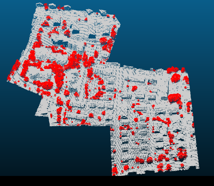
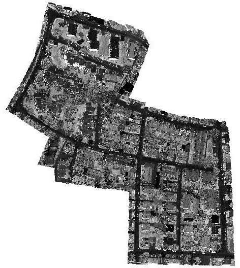
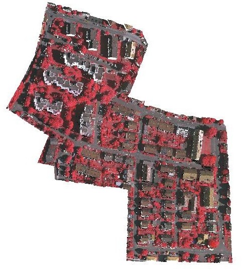
The most accurate tree segmentation results on the ISPRS dataset are visualised in Figure 8 along with the ground truth labels. The results from the proposed methodology suggest that the technique is effective and promising, though not matching the state-of-the-art results. On further analysis of the results, it can be seen that the CNN was able to identify all the large trees but misses the smaller ones. This problem seems to occur due to the voxelisation process when the data is downsampled since some of the smallest trees and bushes occupy a very small number of voxels, making it difficult for them to identify. The best results were achieved when the input data was corrupted by randomly dropping voxels during the training process, improving the generalisation of the network.

IV-C sPointnet++ for Segmentation

TABLE V: sPointnet++ results with varying input types

Input Type	Data Type	$p$	$r$	Fscore
x, y, z	Trees	52	69.5	59.5
x, y, z, i	Trees	51.3	87.3	64.7
x, y, z, i, ir, r, g	Trees	79.5	84.9	82.1
x, y, z	Vegetation	52.2	76.5	62
x, y, z, i	Vegetation	64.9	85.9	73.9
x, y, z, i, ir, r, g	Vegetation	82.9	85.4	84.1

Figure 9: LiDAR data with point intensity in greyscale (left) and combined with spectral information (right).

Figure 10: Area always incorrectly identified by network as tree outline in yellow in spectral image(left) and LiDAR point cloud(right). The LiDAR data is coloured red for all correctly labelled points and blue for all incorrectly labelled ones.

The results of the TreeNet are limited by the voxelisation process, hence Pointnet++ was adapted to work directly on point clouds.

TABLE VI: Comparison of Results on the ISPRS Benchmark Dataset

Method Name Input Type Method Description Precision Recall F1 IIS_7 [42] LiDAR + Orthophoto (XYZRGB) Supervoxel Segmentation + Different ML Classifiers 84 68.8 75.6 WhuY3 [22] Feature Images dervied from LiDAR point cloud 2D CNN 77.5 78.5 78.0 RIT_1 [19] LiDAR points, Spectral Image Pointnet 86.0 79.3 82.5 NANJ2 [21] LiDAR attributes, Geomtrical Features, DTM, Spectral Image Multiscale 2D CNN with Bagged Decision Trees 88.3 77.5 82.6 LUH LiDAR attributes, Geometrical profiles, Textural properties Two Layer CRF 87.4 79.1 83.1 sPointnet++ (Ours) LiDAR, Spectral Image Point cloud based CNN 79.5 84.9 82.1

Figure 11: Visualisation of sPointnet++ output; Left: Ground Truth with trees in red and non-trees in blue, Middle: Output of network (same colour scheme as previously), Right: Error voxels in Purple, correct voxels in Yellow.

The network was trained with different types of input to see the effect of different features. The first type of input was the x, y, z point coordinates, with the x and y inputs normalised per block. For the second input type, the intensity of each point was normalised between 0 and 1 and was concatenated to the point coordinates. For the third input type, the spectral information was added to the point cloud by interpolating the IR-R-G values from the 2D infrared image provided in the ISPRS dataset to the 3D point cloud.

The results of the experiments are summarised in Table V. It can be seen that with only point based inputs, the network was able to recognise 70% of the trees correctly but its precision was low and it falsely identified a number of roofs and shrubs as tree points. The addition of the point intensity value increased the number of trees the network could identify but it still struggled with roofs and shrubs.

To test how well the network was able to identify medium to high vegetation, we also marked all shrubs as positive samples; this gave better results. As can be seen from Table V, the precision in this case was much higher as the shrubs identified as false positives in the previous experiments were now correct and the network had more positive samples to learn from.

Finally, the inclusion of the spectral information along with the point cloud data provided the best results with the top $F_{score}$ of 82.1% (mean 80.48, std dev. 0.877). This was due to the fact that spectral data provides highly discriminating information for identifying vegetation as can be seen in Figure 9, allowing the network to distinguish roofs from vegetation.

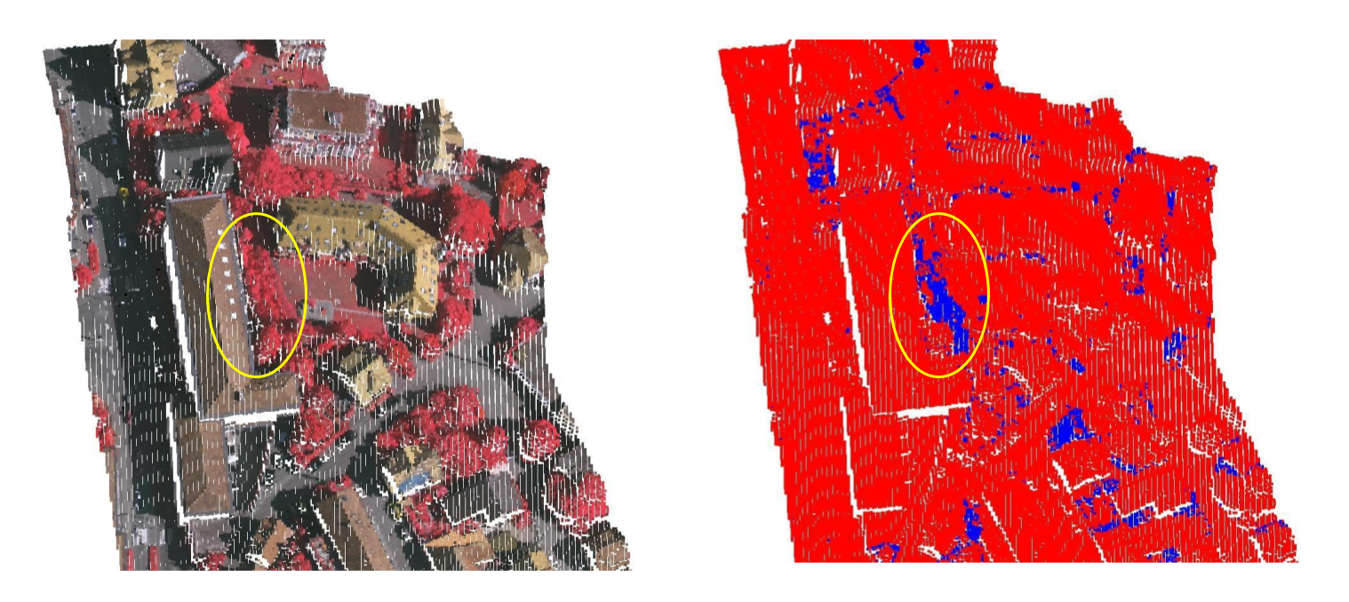
Most misclassifications were shrubs and fences being identified as trees and some points at the edges of trees were missed by the network. The common errors made by all networks are shown in Figure 10, where the area is identified as high vegetation but in the ground truth has been marked as low vegetation. The output from the network is visualised in Figure 11 along with the incorrectly identified points.

We have compared the performance of sPointNet++ on the ISPRS benchmark with other methods in Table VI. The best results on the ISPRS benchmark are only marginally better than that of sPointNet++ but they are a lot more algorithmically intensive. Both LUH and NANJ2 are dependant on a complex preprocessing pipeline to generate geometric features and LUH further uses two independent conditional random fields (CRF) to aggregate the points. RIT_1 averages the results from multiple scales and hence requires multiple passes through their CNN to get multiscale features with $3.7\text{\,}\mathrm{s}$ for 412k points. In contrast, sPointNet++ requires minimal preprocessing of the dataset since it operates directly on the point cloud with spectral information. It also encodes hierarchical information with skip links and only requires a single pass through the CNN with $2.8\text{\,}\mathrm{s}$ for the same data, making it significantly more efficient than the state-of-the-art methods on the ISPRS benchmark.

V Conclusions

In this paper, we have developed and shown both traditional methods and deep learning networks for identifying trees in LiDAR data with disparate resolutions.

The proposed MultiReturn method works on high density LiDAR datasets and utilises the number of returns LiDAR attribute to identify trees. It achieved almost 90% accuracy on the Dublin dataset. Since this method does not scale well to low point-density datasets, we proposed a 3D CNN-based TreeNet to work with a low resolution 3D voxel grid. TreeNet was able to identify large trees in low density datasets but was unable to distinguish small trees due to loss of resolution in the voxelisation process. However, it did show good generalisation capability, since we were able to train on one dataset and test on a completely different dataset (different location, scanning hardware, point cloud statistics, etc).

We also proposed the scaled PointNet++, sPointNet++, which works on spectral data combined with aerial point cloud and does not require voxelisation. The differences in using only point cloud data as compared to point clouds combined with spectral data have been analysed. We achieved comparable results to the state-of-the-art methods in tree identification using point clouds with an $F_{score}$ of 82.1% with a significantly more efficient pipeline.

This work could be improved in several aspects. Ensembles of different models could be used to improve the performance. A larger annotated dataset would also improve performance for sPointNet++, further helping it generalise well. This work could also be extended to multi-class segmentation problems.

References

- The Nature Conservancy [2016] The Nature Conservancy, “Planting Healthy Air,” Tech. Rep., 2016.
- Stoter et al. [2008] J. Stoter, H. de Kluijver, and V. Kurakula, “3D noise mapping in urban areas,” International Journal of Geographical Information Science, vol. 22, no. 8, pp. 907–924, 2008.
- Haala and Kada [2010] N. Haala and M. Kada, “An update on automatic 3D building reconstruction,” ISPRS Journal of Photogrammetry and Remote Sensing, vol. 65, no. 6, pp. 570–580, nov 2010.
- Koch et al. [2006] B. Koch, U. Heyder, and H. Weinacker, “Detection of Individual Tree Crowns in Airborne Lidar Data,” Photogrammetric Engineering & Remote Sensing, vol. 72, no. 4, pp. 357–363, 2006.
- Schwarz [2010] B. Schwarz, “Lidar: Mapping the world in 3D,” Nature Photonics, vol. 4, no. 7, pp. 429–430, jul 2010.
- Hyyppa et al. [2001] J. Hyyppa, O. Kelle, M. Lehikoinen, and M. Inkinen, “A segmentation-based method to retrieve stem volume estimates from 3-D tree height models produced by laser scanners,” IEEE Transactions on Geoscience and Remote Sensing, vol. 39, no. 5, pp. 969–975, may 2001.
- Lu et al. [2014] X. Lu, Q. Guo, W. Li, and J. Flanagan, “A bottom-up approach to segment individual deciduous trees using leaf-off lidar point cloud data,” ISPRS Journal of Photogrammetry and Remote Sensing, vol. 94, pp. 1–12, aug 2014.
- Reitberger et al. [2009] J. Reitberger, P. Krzystek, and U. Stilla, “Benefit of Airborne Full Waveform LIDAR for 3D segmentation and classification of single trees,” in ASPRS 2009 Annual Conference, 2009, pp. 1–9.
- Smits et al. [2012] I. Smits, G. Prieditis, S. Dagis, and D. Dubrovskis, “Individual tree identification using different LIDAR and optical imagery data processing methods,” Biosystems and Information Technology, vol. 1, no. 1, pp. 19–24, 2012.
- Mongus and Zalik [2015] D. Mongus and B. Zalik, “An efficient approach to 3D single tree-crown delineation in LiDAR data,” ISPRS Journal of Photogrammetry and Remote Sensing, vol. 108, pp. 219–233, 2015.
- Secord and Zakhor [2007] J. Secord and A. Zakhor, “Tree Detection in Urban Regions Using Aerial LiDAR and Image Data,” IEEE Geoscience and Remote Sensing Letters, vol. 4, no. 2, pp. 196–200, 2007.
- Chen and Zakhor [2009] G. Chen and A. Zakhor, “2D tree detection in large urban landscapes using aerial LiDAR data,” in Image Processing (ICIP), 2009 16th IEEE International Conference on. IEEE, nov 2009, pp. 1693–1696.
- Carlberg et al. [2009] M. Carlberg, P. Gao, G. Chen, and A. Zakhor, “Classifying urban landscape in aerial lidar using 3D shape analysis,” in Proceedings - International Conference on Image Processing, ICIP. IEEE, nov 2009, pp. 1701–1704.
- Golovinskiy et al. [2009] A. Golovinskiy, V. G. Kim, and T. Funkhouser, “Shape-based recognition of 3D point clouds in urban environments,” in 2009 IEEE 12th International Conference on Computer Vision. IEEE, sep 2009, pp. 2154–2161.
- Höfle et al. [2012] B. Höfle, M. Hollaus, and J. Hagenauer, “Urban vegetation detection using radiometrically calibrated small-footprint full-waveform airborne LiDAR data,” ISPRS Journal of Photogrammetry and Remote Sensing, vol. 67, no. 1, pp. 134–147, jan 2012.
- Liu et al. [2013] J. Liu, J. Shen, R. Zhao, and S. Xu, “Extraction of individual tree crowns from airborne LiDAR data in human settlements,” Mathematical and Computer Modelling, vol. 58, no. 3-4, pp. 524–535, aug 2013.
- Wu et al. [2013] B. Wu, B. Yu, W. Yue, S. Shu, W. Tan, C. Hu, Y. Huang, J. Wu, and H. Liu, “A Voxel-Based Method for Automated Identification and Morphological Parameters Estimation of Individual Street Trees from Mobile Laser Scanning Data,” Remote Sensing, vol. 5, no. 2, pp. 584–611, jan 2013.
- Zhang et al. [2015] C. Zhang, Y. Zhou, and F. Qiu, “Individual Tree Segmentation from LiDAR Point Clouds for Urban Forest Inventory,” Remote Sens, vol. 7, pp. 7892–7913, 2015.
- Yousefhussien et al. [2018] M. Yousefhussien, D. J. Kelbe, E. J. Ientilucci, and C. Salvaggio, “A multi-scale fully convolutional network for semantic labeling of 3D point clouds,” ISPRS Journal of Photogrammetry and Remote Sensing, vol. 143, pp. 191–204, sep 2018.
- Rottensteiner et al. [2014] F. Rottensteiner, G. Sohn, M. Gerke, and J. D. Wegner, “Theme section ”Urban object detection and 3D building reconstruction”,” ISPRS Journal of Photogrammetry and Remote Sensing, vol. 93, pp. 143–144, jul 2014.
- Zhao et al. [2018] R. Zhao, M. Pang, and J. Wang, “Classifying airborne LiDAR point clouds via deep features learned by a multi-scale convolutional neural network,” International Journal of Geographical Information Science, vol. 32, no. 5, pp. 1–20, may 2018.
- Yang et al. [2017] Z. Yang, W. Jiang, B. Xu, Q. Zhu, S. Jiang, and W. Huang, “A convolutional neural network-based 3D semantic labeling method for ALS point clouds,” Remote Sensing, vol. 9, no. 9, 2017.
- Gupta et al. [2018] A. Gupta, J. Byrne, D. Moloney, S. Watson, and H. Yin, “Automatic Tree Annotation in LiDAR Data,” in International Conference on Geographical Information Systems Theory, Applications and Management, 2018.
- Qi et al. [2017a] C. R. Qi, L. Yi, H. Su, and L. J. Guibas, “PointNet++: Deep Hierarchical Feature Learning on Point Sets in a Metric Space,” Neural Information Processing Systems, pp. 601–610, jun 2017.
- Zhang et al. [2003] K. Zhang, S. C. Chen, D. Whitman, M. L. Shyu, J. Yan, and C. Zhang, “A progressive morphological filter for removing nonground measurements from airborne LIDAR data,” IEEE Transactions on Geoscience and Remote Sensing, vol. 41, no. 4 PART I, pp. 872–882, 2003.
- Hobu Inc. [2017] Hobu Inc., “PDAL - Point Data Abstraction Library,” 2017.
- Byrne et al. [2018] J. Byrne, L. Buckley, S. Caulfield, and D. Moloney, “VOLA: A Compact Volumetric Format for 3D Mapping and Embedded Systems,” in Proceedings of the 4th International Conference on Geographical Information Systems Theory, Applications and Management. SCITEPRESS - Science and Technology Publications, 2018, pp. 129–137.
- Nair and Hinton [2010] V. Nair and G. E. Hinton, “Rectified Linear Units Improve Restricted Boltzmann Machines,” in 27th International Conference on Machine Learning, 2010.
- Maas et al. [2013] A. L. Maas, A. Y. Hannun, and A. Y. Ng, “Rectifier nonlinearities improve neural network acoustic models,” in ICML ’13, vol. 28, 2013, p. 6.
- Srivastava et al. [2014] N. Srivastava, G. E. Hinton, A. Krizhevsky, I. Sutskever, and R. Salakhutdinov, “Dropout : A Simple Way to Prevent Neural Networks from Overfitting,” Journal of Machine Learning Research (JMLR), vol. 15, pp. 1929–1958, 2014.
- Moenning and Dodgson [2003] C. Moenning and N. A. Dodgson, “Fast Marching farthest point sampling,” Tech. Rep., 2003.
- Qi et al. [2017b] C. R. Qi, H. Su, K. Mo, and L. J. Guibas, “PointNet: Deep learning on point sets for 3D classification and segmentation,” in Proceedings - 30th IEEE Conference on Computer Vision and Pattern Recognition, CVPR 2017, vol. 2017-Janua, 2017, pp. 77–85.
- Laefer et al. [2015] D. F. Laefer, S. Abuwarda, A.-V. Vo, L. Truong-Hong, and H. Gharibi, “2015 Aerial Laser and Photogrammetry Survey of Dublin City Collection Record,” 2015.
- mon [2015] “LiDAR Aerien Montreal,” 2015. [Online]. Available: http://donnees.ville.montreal.qc.ca/dataset/lidar-aerien-2015
- Ningal [2012] T. Ningal, “PhD Thesis,” Ph.D. dissertation, UCD School of Geography, 2012.
- Cramer [2010] M. Cramer, “The DGPF-Test on Digital Airborne Camera Evaluation – Overview and Test Design,” Photogrammetrie - Fernerkundung - Geoinformation, vol. 2010, no. 2, pp. 73–82, 2010.
- Naus [2006] T. Naus, “Unbiased LiDAR Data Measurement ( Draft ),” 2006.
- GPL Software [2017] GPL Software, “CloudCompare,” 2017.
- Paszke et al. [2017] A. Paszke, S. Gross, S. Chintala, G. Chanan, E. Yang, Z. DeVito, Z. Lin, A. Desmaison, L. Antiga, and A. Lerer, “Automatic differentiation in PyTorch,” 2017.
- Abadi et al. [2015] M. Abadi, A. Agarwal, E. B. Paul Barham, A. D. Zhifeng Chen, Craig Citro, Greg S. Corrado, I. G. Jeffrey Dean, Matthieu Devin, Sanjay Ghemawat, Y. J. Andrew Harp, Geoffrey Irving, Michael Isard, Rafal Jozefowicz, M. S. Lukasz Kaiser, Manjunath Kudlur, Josh Levenberg, Dan Mané, J. S. Rajat Monga, Sherry Moore, Derek Murray, Chris Olah, P. T. Benoit Steiner, Ilya Sutskever, Kunal Talwar, F. V. Vincent Vanhoucke, Vijay Vasudevan, M. W. Oriol Vinyals, Pete Warden, Martin Wattenberg, Yuan Yu, and X. Zheng., “TensorFlow: Large-scale machine learning on heterogeneous systems,” 2015.
- Kingma et al. [2014] D. P. Kingma, D. J. Rezende, S. Mohamed, and M. Welling, “Semi-Supervised Learning with Deep Generative Models,” pp. 1–9, 2014.
- Ramiya et al. [2016] A. M. Ramiya, R. R. Nidamanuri, and K. Ramakrishnan, “A supervoxel-based spectro-spatial approach for 3D urban point cloud labelling,” International Journal of Remote Sensing, vol. 37, no. 17, pp. 4172–4200, sep 2016.