Environmental effects with Frozen Density Embedding in Real-Time Time-Dependent Density Functional Theory using localized basis functions

Abstract

Frozen Density Embedding (FDE) represents a versatile embedding scheme to describe the environmental effect on the electron dynamics in molecular systems. The extension of the general theory of FDE to the real-time time-dependent Kohn-Sham method has previously been presented and implemented in plane-waves and periodic boundary conditions (Pavanello et al. J. Chem. Phys. 142, 154116, 2015).

In the current paper, we extend our recent formulation of real-time time-dependent Kohn-Sham method based on localized basis set functions and developed within the Psi4NumPy framework to the FDE scheme. The latter has been implemented in its “uncoupled” flavor (in which the time evolution is only carried out for the active subsystem, while the environment subsystems remain at their ground state), using and adapting the FDE implementation already available in the PyEmbed module of the scripting framework PyADF. The implementation was facilitated by the fact that both Psi4NumPy and PyADF, being native Python API, provided an ideal framework of development using the Python advantages in terms of code readability and reusability. We employed this new implementation to investigate the stability of the time propagation procedure, which is based an efficient predictor/corrector second-order midpoint Magnus propagator employing an exact diagonalization, in combination with the FDE scheme. We demonstrate that the inclusion of the FDE potential does not introduce any numerical instability in time propagation of the density matrix of the active subsystem and in the limit of weak external field, the numerical results for low-lying transition energies are consistent with those obtained using the reference FDE calculations based on the linear response TDDFT. The method is found to give stable numerical results also in the presence of strong external field inducing non-linear effects. Preliminary results are reported for high harmonic generation (HHG) of a water molecule embedded in a small water cluster. The effect of the embedding potential is evident in the HHG spectrum reducing the number of the well resolved high harmonics at high energy with respect to the free water. This is consistent with a shift towards lower ionization energy passing from an isolated water molecule to a small water cluster. The computational burden for the propagation step increases approximately linearly with the size of the surrounding frozen environment. Furthermore, we have also shown that the updating frequency of the embedding potential may be significantly reduced, much less that one per time step, without jeopardising the accuracy of the transition energies.

1 Introduction

The last decade has seen a growing interest in the electron dynamics taking place in molecules subjected to an external electromagnetic field. Matter-radiation interaction is involved in many different phenomena ranging from weak-field processes, i.e., photo-excitation, absorption and scattering, light harvesting in dye sensitized solar cells ^{1, 2} and photo-ionization, to strong-field processes encompassing high harmonic generation ^{3, 4}, optical rectification ^{5, 6}, multiphoton ionization ⁷ and above threshold ionization ⁸. Furthermore, the emergence of new Free Electron Lasers (FEL) and attosecond methodologies ^{9, 10} opened an area of research in which experiments can probe electron dynamics and chemical reactions in real-time and the movement of electrons in molecules may be controlled. These experiments can provide direct insights into bond breaking ^{11, 12, 13}/forming¹⁴ and ionization ^{15, 16} by directly probing nuclear and electron dynamics.

Real-time time-dependent electronic structure theory, in which the equation of motion is directly solved in the time domain, is clearly the most promising for investigating time-dependent molecular response and electronic dynamics. The recent progress in the development of these methodologies is impressive (see, for instance, a recent review by Li et al.¹⁷). Among different approaches, because of its compromise between accuracy and efficiency, the real-time time-dependent density functional theory (rt-TDDFT) is becoming very popular. The main obstacle to implementing the rt-TDDFT method involves the algorithmic design of a numerically stable and computationally efficient time evolution propagator. This typically requires the repeated evaluation of the effective Hamiltonian matrix representation (Kohn-Sham matrix), at each time step. Despite the difficulties to realizing a stable time propagator scheme, there are very appealing features in a real-time approach to TDDFT, such as the absence of explicit exchange-correlation kernel derivatives  ¹⁸ or divergence problems appearing in response theory and one has the possibility to obtain all frequency excitations at the same cost. Furthermore, the method is suitable to treat complex non-linear phenomena and external fields with an explicit shape, which is a key ingredient for the quantum optimal control theory¹⁹.

Several implementations have been presented ^{20, 21, 22}, after the pioneering work of Theilhaber ²³ and Yabana and Bertsch ²⁴. Many of them rely on the real space grid methodology ²⁴ with Siesta and Octopus as the most recent ones ^{25, 26}. Alternative approaches employ plane waves such as in Qbox ²⁷ or QUANTUM ESPRESSO^{28, 29} and analytic atom centered Gaussian basis implementations (i.e., Gaussian ^{30, 31}, NWChem ³², Q-Chem ^{33, 34}) also have gained popularity. The scheme has been also extended to include relativistic effects at the highest level. Repisky et al. proposed the first application and implementation of relativistic TDDFT to atomic and molecular systems ³⁵ based on the four-component Dirac hamiltonian and almost simultaneously Goings et al. ³⁶ published the development of X2C Hamiltonian-based electron dynamics and its application to the evaluation of UV/vis spectra. Very recently, some of us presented a rt-TDDFT implementation^{37, 38} based on state-of-the-art software engineering approaches (i.e. including interlanguage communication between High-level Languages such as Python, C, FORTRAN and prototyping techniques). The method, based on the design of an efficient propagation scheme within the Psi4NumPy ³⁹ framework, was also extended to the relativistic four-component framework based on the BERTHA code^{40, 41, 42}, (more specifically based on the recently developed PyBERTHA^{37, 38, 43, 44}, that is the Python API of BERTHA).

The applications of the rt-TDDFT approach encompass studies of linear ⁴⁵ and non-linear optical response properties ^{46, 25}, molecular conductance ⁴⁷, singlet-triplet transitions ⁴⁸, plasmonic resonances magnetic circular dichroism ⁴⁹, core excitation, photoinduced electric current, spin-magnetization dynamics ⁵⁰ and Ehrenfest dynamics ^{51, 52}. Moreover, many studies in the relativistic and quasi relativistic framework appeared, ranging from X-ray near-edge absorption ⁵³, to nonlinear optical properties  ⁵⁴, to chiroptical spectroscopy ⁵⁵.

Most part of initial applications of real-time methodology to chemical systems were largely focused on the electron dynamics and optical properties of the isolated target systems. However, it is widely recognized that these phenomena are extremely sensitive to the polarization induced by the environment, such that the simulation on an isolated molecule is usually not sufficient even for a qualitative description. A number of studies aiming at including the effect of a chemical environment within rt-TDDFT have appeared in the literature. They are based on the coupling of rt-TDDFT with the QM/MM approach which includes the molecular environment explicitly and at a reduced cost using classical mechanical description ^{56, 31} or in a polarizable continuous medium (PCM), where the solvent degrees of freedom are replaced by an effective classical dielectric.^{57, 58, 59} One of the challenges, however, in the dynamical description of the environment is that the response of the solvent is not instantaneous, thus these approaches have been extended to include the non-equilibrium solvent response^{60, 61, 62, 63}. A recent extension considers also non-equilibrium cavity field polarization effects for molecules embedded in an homogeneous dielectric⁶⁴.

Going beyond a classical description for the environment, very recently, Koh et al.⁶⁵ have combined the rt-TDDFT method with block-orthogonalized Manby-Miller theory⁶⁶ to accelerate the rt-TDDFT simulations, the approach is also suitable for cheaply accounting the solvation effect on the molecular response. Another fully quantum mechanical approach to include environment effects in the molecular response property is based on the frozen-density embedding (FDE) scheme ^{67, 68, 69}. FDE is a DFT-in-DFT embedding method that allows to partition a larger Kohn-Sham system into a set of smaller, coupled Kohn-Sham subsystems. Additional to the computational advantage, FDE provides physical insight into the properties of embedded systems and the coupling interactions between them.⁷⁰

For electronic ground states, the theory and methodology were introduced by Wesołowski and Warshel ⁷¹, based on the approach originally proposed by Senatore and Subbaswamy ⁷², and later Cortona ⁷³, for solid-state calculations. It has been further generalized ^{74, 75} and directed to the simultaneous optimization of the subsystem electronic densities. Within the linear-response formalism Casida and Wesołowski put forward a formal TDDFT generalization ⁷⁶ of the FDE scheme. Neugebauer ^{77, 78} then introduced coupled FDE, a subsystem TDDFT formulation which removed some of the approximations made in the initial TDDFT-FDE implementations. Recently, the approach has been further extended ^{79, 80} to account for charge-transfer excitations, taking advantage of an exact FDE scheme ^{81, 82, 83, 84, 85}.

A DFT subsystem formulation of the real-time methodology has been presented in a seminal work by Pavanello and coworkers⁷⁰ together with its formulation within the FDE framework. They showed that the extension of FDE to rt-TDDFT can be done straightforwardly by updating the embedding potential between the systems at every time step and evolving the Kohn-Sham subsystems in time simultaneously. Its actual implementation, based on the use of plane-waves and ultrasoft pseudopotentials ^{70, 29}, showed that the updating of the embedding potentials during the time evolution of the electron density does not affect the numerical stability of the propagator. The approach may be approximated and devised in the so called “uncoupled” scheme where the density response to the external field is limited to one active subsystem while keeping the densities of the other subsystems frozen in time. Note that also in this uncoupled version the embedding potential is time-dependent and needs to be recomputed and updated during the time propagation. However, the propagation scheme is restricted to the active subsystem and the approach is promising to include environmental effects in the real-time simulation. Numerous applications within the context of the linear response TDDFT showed that an uncoupled FDE is sufficient for reproducing supermolecular results with good accuracy even in the presence of hydrogen bonds as long as there are no couplings in the excitations between the systems.

In this work we extend rt-TDDFT based on localized basis functions to the FDE scheme in its uncoupled version (uFDE-rt-TDDFT), taking advantage of modern software engineering and code reusability offered by the Python programming language. We devised an unified framework based on Python in which the high interoperability allowed the concerted and efficient use of the recent rt-TDDFT procedure, which some of us have implemented in the framework of the Psi4Numpy API^{37, 38}, and the PyADF API⁸⁶. The rt-TDDFT procedure has served as the main interface where the PyADF methods, which gave direct access to the key quantities necessary to devise the FDE scheme, can be accessed within a unified framework. Since in this work we introduced a new flavor of the rt-TDDFT Psi4Numpy-based program, to avoid confusions, from now on, we will refer to the aforementioned rt-TDDFT based on Psi4Numpy as Psi4-rt, while its extension to the FDE subsystem framework will be referred as Psi4-rt-PyEmbed.

In Section 2 we review the fundamentals of FDE and its extension to rt-TDDFT methodology. In Section 3 computational details are given with a specific focus on the interoperability of the various codes we merged and used: Psi4Numpy³⁹, XCFun⁸⁷ and PyADF⁸⁶, including the PyEmbed module recently developed by some of us. In Section 4 we report and comment the results of the calculations we performed on excitation transitions for different molecular systems, including: a water-ammonia complex, a water cluster and a more extend acetone-in-water cluster case. Finally, we give some preliminary results about the applicability and numerical stability of the method in presence of intense external field inducing strong non-linear effects as High Harmonic Generation (HHG) in the active system. Concluding remarks and perspectives are finally given in Section 5.

2 Theory

In this section we briefly review the theoretical foundations of the FDE scheme and its extension to the rt-TDDFT methodology. As mentioned above, a previous implementation was presented by Pavanello et al. ⁷⁰ using plane waves and ultrasoft pseudopotentials. We refer the interested reader to this seminal work for a general theoretical background, and for additional details of the FDE-rt-TDDFT formal derivation.

2.1 Subsystem DFT and Frozen Density Embedding formulation

In the subsystem formulation of DFT the entire system is partitioned into N subsystems, and the total density $\rho_{\text{tot}}(\bm{r})$ is represented as the sum of electron densities of the various subsystems [i.e., $\rho_{a}(\bm{r})$ ($a=1,..,N$)]. Focusing on a single subsystem, we can consider the total density as partitioned in only two contributions as

$$\rho_{\text{tot}}(\bm{r})=\rho_{\text{I}}(\bm{r})+\rho_{\text{II}}(\bm{r}).$$ (1)

The total energy of the system can then be written as

$$E_{\text{tot}}[\rho_{\text{I}},\rho_{\text{II}}]=E_{\text{I}}[\rho_{\text{I}}]+E_{\text{II}}[\rho_{\text{II}}]+E_{\text{int}}[\rho_{\text{I}},\rho_{\text{II}}]$$ (2)

with the energy of each subsystem ($E_{i}[\rho_{i}]$, with $i=\text{I},\text{II}$) given according to the usual definition in DFT as

$$E_{i}[\rho_{i}] =\int\rho_{i}(\bm{r})v_{\text{nuc}}^{i}(\bm{r}){\rm d}^{3}r+\frac{1}{2}\iint\frac{\rho_{i}(\bm{r})\rho_{i}(\bm{r}^{\prime})}{|\bm{r}-\bm{r}^{\prime}|}{\rm d}^{3}r{\rm d}^{3}r^{\prime}+$$ (3)

$$+E_{\text{xc}}[\rho_{i}]+T_{s}[\rho_{i}]+E_{\text{nuc}}^{i}.$$

In the above expression, $v_{\text{nuc}}^{i}(\bm{r})$ is the nuclear potential due to the set of atoms which defines the subsystem and $E_{\text{nuc}}^{i}$ is the related nuclear repulsion energy. $T_{s}[\rho_{i}]$ is the kinetic energy of the auxiliary non-interacting system, which is, within the Kohn-Sham (KS) approach, commonly evaluated using the KS orbitals. The interaction energy is given by the expression:

$$E_{\text{int}}[\rho_{\text{I}},\rho_{\text{II}}] =\int\rho_{\text{I}}(\bm{r})v_{\text{nuc}}^{\text{II}}(\bm{r}){\rm d}^{3}r+\int\rho_{\text{II}}(\bm{r})v_{\text{nuc}}^{\text{I}}(\bm{r}){\rm d}^{3}r+E^{\text{I,II}}_{\text{nuc}}$$ (4)

$$+\iint\frac{\rho_{\text{I}}(\bm{r})\rho_{\text{II}}(\bm{r}^{\prime})}{|\bm{r}-\bm{r}^{\prime}|}{\rm d}^{3}r{\rm d}^{3}r^{\prime}+E^{\text{nadd}}_{\text{xc}}[\rho_{\text{I}},\rho_{\text{II}}]+T^{\text{nadd}}_{s}[\rho_{\text{I}},\rho_{\text{II}}]$$

with $v_{\text{nuc}}^{\text{I}}$ and $v_{\text{nuc}}^{\text{II}}$ the nuclear potentials due to the set of atoms associated with the subsystem I and II, respectively. The repulsion energy for nuclei belonging to different subsystems is described by the $E^{\text{I,II}}_{\text{nuc}}$ term. The non-additive contributions are defined as:

$$X^{\text{nadd}}[\rho_{\text{I}},\rho_{\text{II}}]=X[\rho_{\text{I}}+\rho_{\text{II}}]-X[\rho_{\text{I}}]-X[\rho_{\text{II}}]$$ (5)

with $X=E_{\text{xc}},T_{s}$. These terms arise because both exchange-correlation and kinetic energy, in contrast to the Coulomb interaction, are not linear functionals of the density.

The electron density of a given fragment ($\rho_{\text{I}}$ or $\rho_{\text{II}}$ in this case) can be determined by minimizing the total energy functional (Eq.2) with respect to the density of the fragment while keeping the density of the other subsystem frozen. This procedure is the essence of the FDE scheme and leads to a set of Kohn-Sham-like equations (one for each subsystem)

$$\Big{[}-\frac{\nabla^{2}}{2}+v^{\text{KS}}_{\text{eff}}[\rho_{\text{I}}](\bm{r})+v_{\text{emb}}^{\text{I}}[\rho_{\text{I}},\rho_{\text{II}}](\bm{r})\Big{]}\phi_{k}^{\text{I}}(\bm{r})=\varepsilon_{k}^{\text{I}}\phi_{k}^{\text{I}}(\bm{r})$$ (6)

which are coupled by the embedding potential term $v^{\text{I}}_{\text{emb}}(\bm{r})$, which carries all dependence on the other fragment’s density. In this equation, $v^{\text{KS}}_{\text{eff}}[\rho_{\text{I}}](\bm{r})$ is the KS potential calculated on basis of the density of subsystem I only, whereas the embedding potential takes into account the effect of the other subsystem (which we consider here as the complete environment). In the framework of FDE theory, $v^{\text{I}}_{\text{emb}}(\bm{r})$ is explicitly given by

$$v^{\text{I}}_{\text{emb}}[\rho_{\text{I}},\rho_{\text{II}}](\bm{r})=\frac{\delta E_{\text{int}}[\rho_{\text{I}},\rho_{\text{II}}]}{\delta\rho_{\text{I}}(\bm{r})}= \ v_{\text{nuc}}^{\text{II}}(\bm{r})+\int\frac{\rho_{\text{II}}(\bm{r}^{\prime})}{|\bm{r}-\bm{r}^{\prime}|}{\rm d}^{3}r^{\prime}+\frac{\delta E_{\text{xc}}^{\text{nadd}}[\rho_{\text{I}},\rho_{\text{II}}]}{\delta\rho_{\text{I}}(\bm{r})}+\frac{\delta T^{\text{nadd}}_{s}[\rho_{\text{I}},\rho_{\text{II}}]}{\delta\rho_{\text{I}}(\bm{r})},$$ (7)

where the non-additive exchange-correlation and kinetic energy contributions are defined as the difference between the associated exchange-correlation and kinetic potentials defined using $\rho_{\text{tot}}(\bm{r})$ and $\rho_{\text{I}}(\bm{r})$. For both potentials, one needs to account for the fact that only the density is known for the total system so that potentials that require input in the form of KS orbitals are prohibited. For the exchange-correlation potential, one may make use of accurate density functional approximations and its quality is therefore similar to that of ordinary KS. The potential for the non-additive kinetic term ($\frac{\delta T^{\text{nadd}}_{s}[\rho]}{\delta\rho_{\text{I}}(\bm{r})}$, in Eq.7) is more problematic as less accurate orbital-free kinetic energy density functionals (KEDFs) are available for this purpose. Examples of popular functional approximations applied in this context are the Thomas-Fermi (TF) kinetic energy functional⁸⁸ or the GGA functional PW91k⁸⁹. These functionals have shown to be accurate in the case of weakly interacting systems including hydrogen bond systems, whereas their use for subsystems interacting with a larger covalent character is problematic (see Ref.⁸¹ and references therein). The research for more accurate KEDFs is a key aspect for the applicability of the FDE scheme as a general scheme, including the partitioning of the system also breaking covalent bonds.⁹⁰

In general, the set of coupled equations that arise in the FDE scheme for the subsystems have to be solved iteratively. Typically, one may employ a procedure of “freeze-and-thaw” where the electron density of the active subsystem is determined keeping frozen the electron density of the others subsystems, which is then frozen when the electron density of the other subsystems is worked out. This procedure may be repeated many times until all subsystems’ densities are converged. In this case the FDE scheme can be seen as an alternative formulation of the conventional KS-DFT approach for large systems (by construction it scales linearly with the number of subsystems). The update of the density for (part of) the environment can be important when trial densities obtained from isolated subsystems are not are not a very good starting point, as is the case for ionic species ^{91, 92, 93}.

The implementation of FDE is relatively straightforward, in that the $v^{\text{I}}_{\text{emb}}(\bm{r})$ potential is a one-electron operator that needs to be added to the usual KS hamiltonian. When using localized basis functions, the matrix representation of the embedding potential (${\bf V^{\text{emb}}}$) may be evaluated using numerical integration grids similar to those used for the exchange-correlation term in the KS method. This contribution is then added to the KS matrix and the eigenvalue problem is solved in the usual self-consistent field manner.

We note that, irrespective of whether one or many subsystem densities are optimized, the matrix ${\bf V^{\text{emb}}}$ needs to be updated during SCF procedure because it also depends on the density of the active subsystem (see Eq.7).

Going beyond the ground state is necessary to access many interesting properties, which for DFT are expressed via response theory^{76, 77, 78, 94, 95}, such as electronic absorption⁹⁶ or NMR shielding^{97, 93}, and for which FDE has been shown to work properly since these are quite often relatively local. In a response formulation, the embedding potential as well as its derivatives enter the equations and, if more than one subsystem is allowed to react to the external perturbations ^{77, 78, 94, 95}, the derivatives of the embedding potential introduce the coupling in the subsystems’ response (as the embedding potential introduces the coupling of the subsystems’ electronic structure in the ground state).

While such couplings in response may be very important in certain situations, such as for strongly interacting systems^{79, 80} or for extensive properties⁷⁸, disregarding them still can provide a very accurate picture, notably for localized excited states^{96, 91}. In this simplified “uncoupled” framework, one considers only the response of the subsystem of interest (and thus the embedding potential and its derivative with respect to this subsystem’s density). While neglecting environment response may seem a drastic approximation, good performance relative to supermolecular reference data has been obtained for excitation energies of a chromophore in a solvent or a crystal environment, even when only retaining the embedding potential ⁹¹. We will therefore employ this framework in the following.

2.2 The Real-Time Time-Dependent Kohn-Sham method and its extension to FDE

The time-dependent equation for the Kohn-Sham method can be conveniently formulated in terms of the Liouville-von Neumann (LvN) equation. In an orthonormal basis set the LvN equation reads:

$$i\frac{\partial\bm{D}(t)}{\partial t}=\bm{F}(t)\bm{D}(t)-\bm{D}(t)\bm{F}(t)$$ (8)

where $i$ is the imaginary unit and $\bm{D}(t)$ and $\bm{F}(t)$ are the one-electron density matrix and time-dependent Kohn-Sham matrix, respectively. The above equation holds in both the non-relativistic and relativistic four-component formulations^{40, 35}.

In a non-relativistic framework, the Kohn-Sham matrix ($\bm{F}(t)$) is defined as

$$\bm{F}(t)=\bm{T}+\bm{v}_{\text{nuc}}+\bm{V}_{\text{xc}}[\rho(t)]+\bm{J}[\rho(t)]+\bm{v}_{\text{ext}}(t),$$ (9)

where $\bm{T}$ and $\bm{v}_{\text{nuc}}$ are the one-electron non-relativistic kinetic energy and intramolecular nuclear attraction terms, respectively. The explicit time dependence of $\bm{F}(t)$ is due to the time-dependent external potential $\bm{v}_{\text{ext}}(t)$, which accounts for the interaction of the molecular system with an applied external electric field. Even in the absence of an external field the Fock operator is implicitly dependent on time through the density matrix $\bm{D}(t)$ in the Coulomb ($\bm{J}[\rho(t)]$) and exchange-correlation terms ($\bm{V}_{\text{xc}}[\rho(t)]$).

The propagation in time of the density matrix can be expressed as

$$\bm{D}(t)=\bm{U}(t,t_{0})\,\bm{D}(t_{0})\,\bm{U}(t,t_{0})^{\dagger}$$ (10)

where $\bm{U}(t,t_{0})$ is the matrix representation of the time-evolution operator.

If we start (initial condition, i.e. initial time $t_{0}$) with the electronic ground state density matrix and use as orthonormal basis the ground state molecular orbitals, $\bm{D}(t_{0})$ assumes the form

$$\bm{D}(t_{0})=\begin{pmatrix}\bm{1}_{oo}&\bm{0}_{ov}\\ \bm{0}_{vo}&\bm{0}_{vv}\end{pmatrix}\\ \quad,$$

where $\bm{1}_{oo}$ is the identity matrix over the occupied orbital space of size $n_{occ}$ (total number of electrons). The $\bm{D}$ matrix has the dimension of $n_{\text{tot}}$ ($n_{\text{tot}}=n_{occ}+n_{virt}$) that is total number of the basis functions.

In our implementation, which uses a basis set of atomic centered (AO) Gaussian-type functions, the ground-state molecular orbitals are conveniently used as the reference orthonormal basis and at the time $t$ the Fock and density matrices are related to their AO basis representation simply by:

$$\bm{F}(t)^{MO}=\bm{C}^{\dagger}\bm{F}(t)^{AO}\bm{C}$$ (11)

where the $\bm{C}$ matrix contains the reference MO expansion coefficients. The same coefficients satisfy a similar relation for $\bm{D}(t)^{MO}$:

$$\bm{D}(t)^{AO}=\bm{C}\bm{D}(t)^{MO}\bm{C}^{\dagger}$$ (12)

In a finite time interval, the solution of the Liouville-von Neumann equation consists in the calculation of the Fock matrix at discrete time steps, and in propagating the density matrix in time.

In the most general case, where the Fock operator depends on time even in absence of external fields, the time-evolution operator can be expressed by means of a Dyson-like series:

$$\bm{U}(t,t_{0})=\sum_{n=1}^{\infty}\frac{(-i)^{n}}{n!}\int_{t_{0}}^{t}d\tau_{1}\int_{t_{0}}^{t}d\tau_{2}\ldots\int_{t_{0}}^{t}d\tau_{n}\bm{F}(\tau_{1})\bm{F}(\tau_{2})\ldots\bm{F}(\tau_{n})$$ (13)

$$\tau_{1}>\tau_{2}\ldots>\tau_{n}$$

which in compact notation, using the the time ordering operator $\hat{\mathcal{T}}$, reads as:

$$\bm{U}(t,t_{0})=\hat{\mathcal{T}}\exp\bigg{(}-i\int_{t_{0}}^{t}\bm{F}(t^{\prime})dt^{\prime}\bigg{)}$$ (14)

The time ordering is necessary since $\bm{F}(t)$ at different times do not necessarily commute ($[\bm{F}(t),\bm{F}(t^{\prime})]\neq 0$). Typically, this time-ordering problem is overcome by exploiting the composition property of time-evolution operator ($\bm{U}(t,t_{0})=\bm{U}(t,t_{1})\bm{U}(t_{1},t_{0})$) and discretizing the time using a small time step. It is clear that the exact time ordering can be achieved only in the limit of an infinitesimal time step. Many different propagation schemes have been proposed⁹⁸ in the context of rt-TDDFT. Among others, we mention the Crank-Nicholson ⁹⁹, Runge-Kutta ¹⁰⁰ or Magnus ^{101, 102} methods.

The Magnus expansion has found the widest application, in particular, in those implementations that employ localized basis sets functions, for which matrix exponentiation can be performed exactly via matrix diagonalization. Typically, the Magnus expansion is truncated to the first order evaluating the integral over time using numerical quadrature, provided that the time interval $\Delta t$ is sufficiently short. Using the midpoint rule the propagator becomes

$$\bm{U}(t+\Delta t,t)\approx\exp\bigg{[}-i\bm{F}\Big{(}t+\frac{\Delta t}{2}\Big{)}\Delta t\bigg{]}.$$ (15)

This approach, also referred as second-order midpoint Magnus propagator, is unitary by construction, provided that $\bm{F}$ is hermitian. This scheme exhibits an error which is proportional to $(\Delta t)^{3}$. The expression in Eq.15 coincides with the so-called modified-midpoint unitary transform time-propagation scheme originally introduced by Schlegel et al.²¹.

The $\bm{F}$ matrix at time $t+\Delta t/2$, where no density is available, can be obtained using an iterative series of extrapolations and interpolations at each time. Note that, if this predictor/corrector procedure is converged in a self-consistent manner the second-order midpoint Magnus propagator preserves the time reversal symmetry, which is an exact property of the equation of motion in absence of magnetic field. The predictor/corrector scheme is a key ingredient in preserving the numerical stability of the propagation with a range of algorithms that can be applied in this context ¹⁰³. We have recently implemented a particularly stable predictor/corrector scheme, originally proposed by Repiskyet al.³⁵, in the interactive quantum chemistry programming environment Psi4NumPy^{39, 37, 38}.

The methodology that we have described above can be straightforwardly extended to the subsystem density functional theory framework and in particular to FDE (FDE-rt-TDDFT)⁷⁰. In the present work we consider one active subsystem and keep frozen the density of the environment along the time propagation (uncoupled scheme, to which we will refer as uFDE-rt-TDDFT). Thus, a LvN type equation is solved in the space of the active subsystem. The only modification to Eq.8 is in the definition of the effective hamiltonian matrix representation which now refers to the active subsystem ($\bm{F}^{\text{I}}(t)=\bm{T}^{\text{I}}+\bm{v}_{\text{nuc}}^{\text{I}}+\bm{V}_{\text{xc}}[\rho^{\text{I}}(t)]+\bm{J}[\rho^{\text{I}}(t)]+\bm{v}_{\text{ext}}(t)$) and to which the matrix representation of the embedding potential ($\bm{V}^{\text{emb}}(t)$) is added to take into account the effect of the environment. The propagation scheme itself remains unaltered.

As in the case for the ground state, in which the change of the active subsystem density requires that $\bm{V}^{\text{emb}}$ is updated at each SCF iteration, the time propagation of the electron density will introduce a time dependence in $\bm{V}^{\text{emb}}$ even though the environment densities are kept frozen at their ground state value (due to the use of the uncoupled scheme).

Thus, the $\bm{V}^{\text{emb}}$ matrix needs to be updated during the propagation. In the present implementation we use atomic centered Gaussian function as basis set for the active subsystem and evaluate the $V^{\text{emb}}_{\mu\nu}$ matrix elements numerically ⁹¹. We will show that the numerical noise associated with the construction of the embedding potential introduced by this scheme does not affect the numerical stability of the density matrix propagation in the linear and non-linear regimes. In the following sections we will also demonstrate, for a specific application, that the updating frequency of the embedding potential may be significantly reduced (much less than one per time step used to solve the LvN equation) without jeopardising the accuracy.

As usual, the key quantity in a real time simulation is the time-dependent electric dipole moment ${\vec{\mu}}(t)$. Each Cartesian component $p$ (with $p=x,y,z$) is given by

$${\mu_{p}}(t)=-\int\rho(t,{\bf r})p\,d{\bf r}=\mathrm{Tr}(\bm{D}(t)\bm{P}_{p}),$$ (16)

where $\bm{P}_{p}$ is the matrix representation of the p-th component of the electric dipole moment operator (see also Eq. 16). Since, in our uFDE-rt-TDDFT implementation, the time dependency response of the external field is due only from the active system, in the above expression (Eq.16) all quantities refer to the active subsystem. The vector ${\vec{\mu}}(t)$ defines the polarization response to all orders and is easily computed by the electronic density at any time, $t$. From this quantity one can then compute both linear and non-linear properties.

In the linear response regime, each component of electric dipole moment, $\mu_{p}(\omega)$, with an external field $E_{q}$ in the direction $q$ (with $q=x,y,z$), is given in frequency space by

$$\mu_{p}(\omega)=\sum_{q}\alpha_{pq}(\omega)E_{q}(\omega).$$ (17)

The components depend on the polarizability tensor ($\alpha_{pq}$) through the Fourier-transformation of the $q$-component of the applied field. The dipole strength function $\mathrm{S}(\omega)$ is related to the imaginary part of the frequency dependent linear polarizability by

$$\mathrm{S}(\omega)=\frac{2\omega}{3\pi}\mathrm{Im\,Tr}[\alpha(\omega)]$$ (18)

In our implementation³⁷ the perturbation can be chosen to be either an impulsive kick or a continuous wave whose amplitude is modulated by an analytic envelope function. Different explicit functional forms are available ^{37, 38}. In the case of an impulsive perturbation (${\bf E}(t)=k\delta(t)$${\bf n}$, where ${\bf n}$ is a unit vector representing the orientation of the field) we adopt the $\delta$-analytic representation as proposed in Ref. ³⁵. One of the best-known examples of non-linear optical phenomena is HHG in atoms and molecules. HHG occurs via photo-emission by the molecular system in a strong field and can be also computed from ${\vec{\mu}}(t)$ ¹⁰⁴. In this work we calculate the HHG power spectrum for a particular polarization direction as the Fourier transform of the laser-driven induced dipole moment,

$$P(\omega)\propto\Bigg{|}\int_{t_{1}}^{t_{2}}\mu_{z}(t)\exp(-i\omega t)dt\Bigg{|}^{2}.$$ (19)

Other suitable approaches have been investigated in the literature¹⁰⁴, but in all cases the key quantity is ${\vec{\mu}}(t)$.

3 Computational Details and Implementation

In this section we outline the computational strategy we adopted to implement the uFDE-rt-TDDFT scheme. We devised a multi-scale approach where we take advantage of the real-time TDDFT reference procedure, recently implemented within Psi4Numpy framework (i.e. Psi4-RT program)^{37, 38}, while the FDE computational core relies on PyADF^{86, 105} and makes use of its PyEmbed module, which some of us have recently developed ^{106, 107}. PyEmbed provides a Python implementation for computing the interaction energy (Eq. 4) and embedding potential (Eq. 7) from FDE on user-defined integration grids, while using the XCFun library^{18, 87} to evaluate non-additive xc and kinetic energy contributions. With PyEmbed, quantum chemistry codes require only minimal changes: functionality to provide electron densities and its derivatives, as well as the electrostatic potential, over the grid, as well as to read in the embedding potential, and add it as a one-electron operator in the Fock matrix⁹¹. The PyADF scripting framework provides all the necessary tools to manage various computational tasks and manipulate the relevant quantities for electronic-structure methods. The resulting Python code, referred as Psi4-rt-PyEmbed, is available under GPLv3 license at Ref. 108. A data set collection of computational results, including numerical data and parameters used to obtain the absorption spectra of Sections 4.2, 4.3 and 4.5, is available in the Zenodo repository and can be freely accessed at Ref.  109.

3.1 Rapid prototyping and implementation

Psi4Numpy ^{39, 110} and PyADF ^{86, 105}, both provide a Python interface, which greatly simplifies the computational work-flow from input data to the results. PyADF is a quantum chemistry scripting framework that provides mechanisms for both controlling the execution of different computational tasks and for managing the communication between these tasks using Python object-oriented programming techniques. As we already mentioned, its built-in classes permit to handle different aspects involved in the work-flow as a single unit. All the advantages coming from object-oriented programming (i.e extensibility and inheritance) are readily available and allow us to incorporate third-party scientific code and directly manipulate quantities coming from different codes (Psi4Numpy) in our case.

The Python HLL (High-Level Language), among others, permits to formally express complex algorithms in comparatively few lines of codes. This makes rather straightforward to let PyADF interact with Psi4Numpy native Python API. For the sake of completeness we want to finally mention that, to accomplish our goal, we firstly had to port some of the frameworks (specifically XCFun, PyADF and PyEmbed) to the new Python 3.0 standard (i.e., we used a private branch of the cited packages, available at Refs. 111, 112).

As an explicit example of the interoperativity achieved between different codes we report in Algorithm 1 some basic directives used to compute those key quantities necessary for our uFDE-rt-TDDFT. The electron density of an active system is obtained via Psi4Numpy while the electron density, the Coulomb potential and non-additive terms of the environment are managed using PyADF. These quantities can be easily mapped on a common numerical grid and used in PyEmbed to evaluate the relative non additive embedding potential. Thus, the geometry and basis set of the active system (in this specific case a H₂O molecule) are parsed at Line 7 and the ground state wavefunction object is returned by the psi4.energy() method. The corresponding electron density matrix is then obtained as a NumPy array by the h2o_wfn object. The electron density is mapped into a real-space grid representation using a preset numerical grid, and used to populate a suitable object container (Line 14-20). A ground state calculation of the environment molecule (that is a NH₃ molecule in this example) is carried out using PyADF run() method (Line 23). In this case we use the adfsinglepointjob method to execute the corresponding ADF calculation¹¹³. We mention here that PyADF, despite its name, is not specific to this program, but works with a number of different quantum chemistry codes. The density and Coulomb potential resulting from this calculation, that are represented on a common numerical grid, are obtained using get_density() and get_potential() methods (Line 25,27) respectively. The PyEmbed module has all the methods needed to manage the density of both the reference system and environment to finally compute the non-additive embedding potential. Indeed, the embed_eval object is instantiated (Line 34) and the non-additive embedding potential is evaluated on the numerical grid using get_nad_pot (Line 36), once the density of both the active system and of the environment has been provided.

1:  import psi4

2:  import pyadf

3:  import pyadf.PyEmbed

4:  from pyadf.Plot.GridFunctions import GridFunctionFactory

5:  from pyadf.Plot.GridFunctions import GridFunctionContainer

6:  …

7:  geom,mol = fde_util.set_input(’h2o.xyz’,basis_set)

8:  # psi4 run

9:  ene, h2o_wfn = psi4.energy(func,return_wfn=True)

10:  # get psi4 h2o density

11:  D = np.array(h2o_wfn.Da())

12:  …

13:  # map h2o density matrix to the numerical grid

14:  temp = 2.0 * fde_util.denstogrid( phi, D, S,ndocc)

15:  rho = np.zeros((temp.shape[0],10),dtype=np.float_)

16:  rho[:,0] = temp

17:  # fill in the container with density

18:  dens_gf = GridFunctionFactory.newGridFunction(agrid, np.ascontiguousarray(rho[:,0]),gf_type="density")

19:  …

20:  density_h2o = GridFunctionContainer([dens_gf, densgrad, denshess])

21:  m_nh3 = pyadf.molecule(nh3.xyz)

22:  # ADF run

23:  run_nh3 = pyadf.adfsinglepointjob(m_nh3, basis_active, settings=adf_settings, options=[’NOSYMFIT’]).run()

24:  # get nh3 density

25:  density_nh3 = run_nh3.get_density(grid=agrid, fit=False, order=2)

26:  # get nh3 coulomb potential

27:  nh3_coul = run_nh3.get_potential(grid=agrid, pot=’coul’)

28:  …

29:  

30:  # PyEmbed run

31:  embed_settings = pyadf.PyEmbed.EmbedXCFunSettings()

32:  embed_settings.set_fun_nad_xc ({’BeckeX’: 1.0, ’LYPC’: 1.0})

33:  embed_settings.set_fun_nad_kin({’pw91k’ : 1.0})

34:  embed_eval = pyadf.PyEmbed.EmbedXCFunEvaluator(settings=embed_settings)

35:  # compute non-additive part of the embedding potential

36:  nadpot_h2o = embed_eval.get_nad_pot(density_h2o, density_nh3)

37:  nad_val = nadpot_h2o.get_values()

Algorithm 1 Illustrative Python code to compute active system density (using the Psi4Numpy code), environment density and Coulomb potential (using the ADF code) and non-additive embedding potential via the PyEmbed module.

Algorithm 1 has well illustrated how we can utilize the classes provided by PyADF to obtain a very simple workflow in which we are able to manipulate quantities coming from Psi4Numpy. Thus, we are now in a position to draw the main lines of our uFDE-rt-TDDFT implementation, the Psi4-RT-PyEmbed code¹⁰⁸. In Figure 1 we present its pictorial workflow.

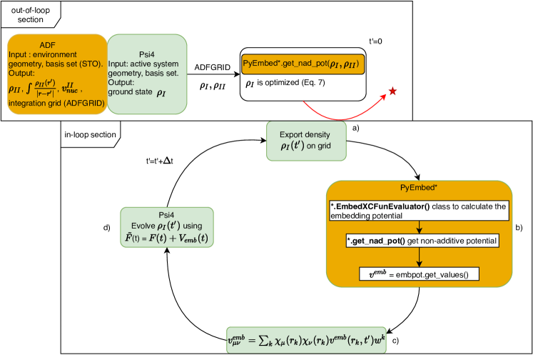
Figure 1: Working flowchart of the uFDE-RT-TDDFT. In the out-of-loop section the density and electrostatic potential of the environment are obtained as grid functions. The active system density matrix is expressed as grid function object and used to calculate the embedding potential. The active system density is optimized self-consistently according to Eq 7. The red star and the arrow pointing at it, symbolize that the out-of-loop blocks of tasks are involved only in the initial stage of the procedure. a) The relaxed active density matrix is exported as grid function. b) PyEmbed classes are used to calculate the embedding potential. c) The embedding potential is expressed on the finite basis set representation (GTO’s). d) The active density matrix is evolved according to the real-time propagation scheme.

We start describing the out-of-loop section. Firstly the geometry and basis set of the environment are initialized (the orange left most block), thus the ADF package provides, through a standalone single point calculation, the electrostatic and nuclear potential of the environment and its density $\rho_{\text{II}}$ and a suitable integration grid for later use. At this stage all the basis sets and exchange-correlation functionals available in the ADF library can be used. In the next step, green block, the geometry and basis set of the active system are parsed from input and the ground state density $\rho_{\text{I}}$ is calculated using the Psi4Numpy related methods. The right pointing arrow, connecting the last block, sketches the mapping of the density matrix onto the real-space grid representation. The evaluation of $\rho_{\text{I}}(\bm{r})$ on the numerical grid is efficiently accomplished using the molecular orbitals (MO), which requires the valuation the localized basis functions at the grid points.

Finally, the PyEmbed module comes into play (last block of the out-of-loop section), the real-space electron densities $\rho_{\text{I}}$ and $\rho_{\text{II}}$ serve as input for the get_nad_pot() method. Thus the non-additive kinetic and exchange potential are obtained. The embedding potential is then calculated from its constituents (i.e. the environment electrostatic and nuclear potential and the non-additive contribution as detailed in Eq. 7) and evaluated at each grid point, $v^{\text{emb}}(\bm{r}_{k})$. The embedding potential matrix representation in the active subsystem basis set, $\bm{V}^{\text{emb}}$, is calculated numerically on the grid as

$$V_{\mu\nu}^{\text{emb}}=\sum_{k}\chi_{\mu}(r_{k})\chi_{\nu}(r_{k})v^{\text{emb}}(r_{k})w_{k}$$ (20)

where $\chi_{\mu}(\bm{r}_{k})$ are the Gaussian-type basis set functions employed in the active systems (used in Psi4Numpy) evaluated at the grid point, $\bm{r}_{k}$. In the above expression, $w_{k}$ are specific integration weights.

In the case of a FDE-rt-TDDFT calculation, the electron density of the active system at the beginning of the propagation ($t_{0}=0$, initial condition) is not the ground state density of the isolated molecule, rather a polarized ground state density. The latter is obtained through a self-consistent-field calculation in the presence of the embedding potential. We adopt the so-called split-scf scheme as described in Ref. 114. It should be noted that the density matrix, corresponding to the optimized $\rho_{\text{I}}$ electron density, is the input data for the green block (block a) of the in-loop section. The outgoing red arrow, connecting the out- and the in-loop branch of the diagram, it means that the former is only involved in the early step of the procedure and it will no longer come into play during the time propagation. As mentioned, the optimized density matrix of the active system as resulting from the SCF procedure including the embedding potential, is the starting point for the real-time propagation. Whereupon, at each time step we determine the embedding potential corresponding to the instantaneous active density ($v^{\text{emb}}[\rho_{\text{I}}(t),\rho_{\text{II}}]$). Again we need its mapping onto the real-space grid as shown in the first green box (box a). Then, we utilize the methods reported in the rectangular orange box (box b) to calculate the non-additive part of the embedding potential at each grid point. Finally we add the non-additive (kinetic and exchange-correlation) potential to the electrostatic potential of the environment calculated again at each grid point. It should be noted that because the density of the environment is frozen, thus the corresponding electrostatic potential remains constant during the time propagation. In the next phase its matrix representation in the localized Gaussian basis functions is obtained as in Eq.20, (box c, in Figure). The active system is evolved (box d) using an effective time-dependent Kohn-Sham matrix, which contains the usual implicit and explicit time-dependent terms, respectively (J$[\rho_{\text{I}}(t)]$+V_XC$[\rho_{\text{I}}(t)]$) and v${}_{\mathrm{ext}}(t)$, plus the time-dependent embedding potential ($\bm{V}^{\text{emb}}[\rho_{\text{I}}(t),\rho_{\text{II}}]$).

For the sake of completeness, the pseudo code needed to evolve the density using the second-order midpoint Magnus propagator is reported in SI and relies on the methodology illustrated in Section 2.2. We refer the interested readers to our recent work on real-time propagation for further details ³⁷.

4 Results and Discussion

In the present section we report a series of results mainly devoted to assess the correctness of the uFDE-rt-TDDFT scheme. To the best of our knowledge, this implementation is the first available for localized basis sets. Since our implementation relies on the embedding strategies implemented in PyADF, it appears natural and appropriate to choose as a useful reference the uncoupled FDE-TDDFT scheme, based on the linear response^{115, 75} and implemented in the ADF program package ¹¹⁶.

4.1 Initial validation and numerical stability

Before going into the details of the numerical comparison between our implementation and the FDE-TDDFT scheme based on the linear response (ADF-LR) formalism, whether in combination with FDE (ADF-LR-FDE) or not, is important to first assess the basis set dependence of the calculated excitation energies using the two different approaches. This preliminary study is mandatory because Psi4Numpy (Gaussians) and ADF (Slaters) employ different types of atom-centered basis functions. Due to this difference, perfect numerical agreement between the two implementations can not be expected, but it is important to quantify the variability of our target observables (the excitation energies of a water molecule) with variations in the basis set.

In order to simulate the linear response regime within our Psi4-rt, the electronic ground-state of a water molecule, calculated in absence of an external electric field, was perturbed by an analytic $\delta$-function pulse with a strength of $\kappa=$ 1.0$\times 10^{-5}$ a.u. along the three directions, $x,y,z$. The induced dipole moment has been collected for 9000 time steps with a length of 0.1 a.u. per time step, corresponding to 21.7 fs of simulation. This time dependent dipole moment is then Fourier transformed in order to obtain the dipole strength function $S(w)$, accordingly to Eq. 18 and the transition energies. The Fourier transform of the induced dipole moment has been carried out by means of Padé approximants ^{117, 17}.

As shown in Table 1, convergence can be observed with both Psi4-rt and ADF-LR, in particular for the first low-lying transitions (additional excitation energies are reported in the Supporting Information). For some of the higher energy transitions the convergence is less prominent, pointing to deficiencies in the smaller basis sets. We mention that the results obtained using our Psi4-rt implementation perfectly agree with those obtained using the TDDFT implementation based on linear response implemented in the NWChem code, which uses the same Gaussian type basis set (see Table S1 in SI). Thus, we conclude that most of the deviations from the ADF-LR values can be ascribed to unavoidable basis set differences. A qualitatively similar pattern of differences is to be expected when including the environment effect within the FDE framework.

Table 1: Excitation energies (in eV) corresponding to the first five low-lying transitions of the isolated water molecule. Data obtained using TDDFT based on linear response implemented in ADF (ADF-LR) and the our real-time TDDFT implemented (Psi4-rt). The labels (D, T, Q) correspond to data obtained using the Gaussian-type basis sets aug-cc-pVXZ (X = D,T,Q) and Slater-type basis sets AUG-X^′ (X^′ = DZP,TZ2P,QZ4P) which are used in the Psi4-rt and ADF-LR codes, respectively (see text for details).

Excitation energy (e.V)
Psi4-rt   ADF-LR
	D	T	Q		D	T	Q
Root 1	6.2144	6.2269	6.2244		6.1610	6.1887	6.2868
Root 2	7.5125	7.4660	7.4404		7.4540	7.4646	7.8841
Root 3	8.3626	8.3516	8.3436		8.3088	8.2881	8.4267
Root 4	9.5357	8.9526	8.6506		8.8033	8.4825	8.6276
Root 5	9.6436	9.5721	9.3056		8.9446	8.8453	10.022

To assess differences in the presence of an environment, we next tested our uFDE-rt-TDDFT results against ADF-LR-FDE ones. The target system is the water-ammonia adduct, in which the water molecule is the active system that is bound to an ammonia molecule, which plays the role of the embedding environment. In the Psi4-rt-PyEmbed case we employed a contracted Gaussian aug-cc-pVXZ (X=D,T) basis set ^{118, 119} for the active system whereas the basis set used in PyADF for the calculation of the environment frozen density (ammonia) and the embedding potential is the AUG-X^′ (X^′=DZP,TZ2P) Slater-type set from the ADF library¹¹⁶. The ADF-LR-FDE employs the AUG-X^′ (X^′=DZP,TZ2P) basis sets from the same library. For the real-time propagation of the active system (water), in both the isolated and the embedded case the BLYP ^{120, 121} exchange-correlation functional is used, while the Thomas-Fermi and LDA functionals ^{122, 123} have been employed for the non-additive kinetic and non-additive exchange-correlation potentential, respectively. The numerical results are reported in Table 2. Although, as expected, there is no quantitative agreement on the absolute value of the transitions, the shift $\Delta$ ($E_{iso.}-E_{\text{emb}}$) shows an acceptable agreement for the lowest transitions (see for additional excitation energies the Supporting Information).

Table 2: Excitation energies (in eV) corresponding to the first five low-lying transitions of both the isolated and embedded calculations water molecule are reported. In the embedded water molecule, an ammonia molecule is used as environment. Data have been obtained using our new Psi4-rt-PyEmbed implementation and reference ADF-LR-FDE implementation with (a) aug-cc-pVDZ and AUG-DZP basis sets; and (b) aug-cc-pVTZ and AUG-TZ2P basis sets (see text for details). The shift $\Delta$ ($E_{iso.}-E_{\text{emb}}$) in the transition energies due to the embedding environment is also reported.

Excitation energy (e.V)
Psi4-rt-PyEmbed   ADF-LR-FDE
	isolated	emb.	$\Delta$		isolated	emb.	$\Delta$
(a) double-zeta calculations
Root 1	6.2144	5.8167	0.398		6.1610	5.6871	0.474
Root 2	7.5125	6.6940	0.818		7.4540	6.5779	0.876
Root 3	8.3626	7.8924	0.470		8.3088	7.7818	0.527
Root 4	9.5357	8.7677	0.768		8.8033	8.3361	0.467
Root 5	9.6436	9.1861	0.458		8.9446	8.4215	0.523
(a) triple-zeta calculations
Root 1	6.2269	5.7964	0.4305		6.1887	5.6886	0.500
Root 2	7.4660	6.5734	0.8926		7.4646	6.5592	0.905
Root 3	8.3516	7.8485	0.5031		8.2881	7.7339	0.554
Root 4	8.9526	8.5596	0.3930		8.4825	7.9692	0.513
Root 5	9.5721	8.6246	0.9475		8.8453	8.3180	0.527

From these results, we conclude that our implementation is both stable and numerically correct, with differences between the methods explainable by the intrinsic basis set differences.

4.2 The water in water test case

To provide a further test of our implementation, we also computed the absorption spectra of a water molecule embedded in a water cluster of increasing size. The geometries of the different water clusters are taken from Refs. ^{124, 125} which corresponds to one snapshot taken from a MD simulation. Different cluster models were taken in consideration, by progressive addition of surrounding water molecules (from 1 to 5 molecules) to the single active water molecule. For the active system water molecule propagation in Psi4-rt-PyEmbed we use the aug-cc-pVDZ basis set while for the environment, computed using the ADF code, we use the AUG-DZP basis set. In both cases we use the BLYP ^{120, 121} exchange-correlation functional while for the non-additive kinetic and non-additive exchange-correlation terms in the generation of the embedding potential the Thomas-Fermi and LDA functionals are used, respectively. In each case, we use 9000 time steps of propagation which corresponds to a simulation of $\approx$ 22 fs (time step of 0.1 a.u.). The corresponding dipole strength functions ($S_{z}(w)=2w/(3\pi)\mathrm{Im}[\alpha_{zz}(w)]$) along the $z$-direction are reported in Fig. 3. Upon the increase of the cluster dimension, the lowest-lying transition shifts within a range of about 1 eV and no spectra display cusps or irregular behavior. These results give confidence in the numerical stability of the propagation when the number of molecules in the environment is increased.

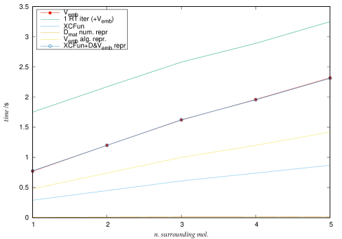
Figure 2: Time needed for different tasks vs number of surrounding molecules

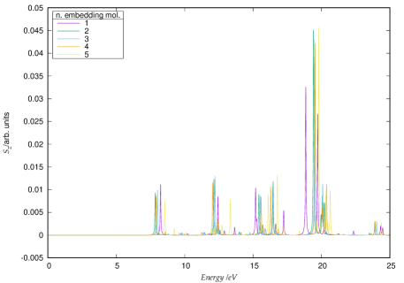
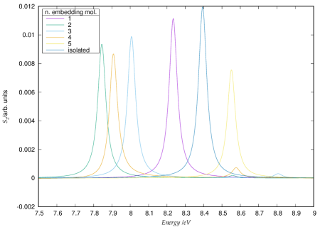
Figure 3: Dipole strength function $S_{z}$ of the water cluster as a function of the number of surrounding molecules (left panel). Right panel: detailed representation of the low lying transition. The peak corresponding to the isolated molecule is reported for comparison

The systematic increase of the size of the environment makes it possible to also consider the actual computational scaling of the Psi4-rt-PyEmbed code for this case. To show this scaling, we carried out a single time step of the real-time propagation and broke down the computational cost into those of the different steps in the work-flow, as reported in Fig. 1.

Table 3: Time usage in seconds. ^a : Density on grid (through MOs). ^b : XCFun (non-additive potential calculation). ^c : V${}_{\text{emb}}$ projection onto the basis set ^d : Total time for V${}_{\text{emb}}$ evaluation. ^e : Total time for a rt-iteration

	ta	tb	tc	td	te
1	0.007	0.29	0.48	0.77	1.75
2	0.01	0.45	0.74	1.20	2.17
3	0.014	0.61	1.0	1.62	2.58
4	0.015	0.74	1.2	1.96	2.89
5	0.02	0.87	1.42	2.32	3.25

In Table 3, and in Fig.2, we report how the time for the embedding potential calculation is distributed over the different tasks, when the number of surrounding water molecules increases from one to five. It is interesting to note that the time needed to evaluate the embedding potential increases almost linearly, for the limited number of water molecules considered here. The standard real-time iteration time (corresponding to the isolated water molecule) takes less than 1 sec and shows up as a fixed cost in the increasing computation time, while the time spent in the embedding part is dominated by the evaluation of the matrix representation for the active subsystem, e.g step c) of Fig.1 (see for instance t^c column of Table 3). The time spent in this evaluation depends on the number of numerical integration points used to represent the potential, and can be reduced by using special grids for embedding purposes once the environment is large enough.

4.3 The acetone in water test case

As a further test of the numerical stability of accuracy of the method, we investigated the $n\to\pi^{*}$ transition in the acetone molecule, both isolation and using an explicit water cluster to model solvation. In order to assess the shift due to the embedding potential, we calculate the absorption spectrum of the isolated molecule at the same geometry it has in the cluster model. The geometry for the solvated acetone system was taken from Ref. 91, corresponding to one snapshot from a MD simulation, where the acetone is surrounded by an environment consisting of 56 water molecules. The uFDE-rt-TDDFT calculation has been obtained specifying in our Psi4-rt-PyEmbed framework all the computational details. In particular, the frozen density of the environment is obtained from a ground state calculation using ADF in combination with the PBE functional and DZP basis set, while for the acetone we employ the BLYP functional and the Gaussian def2-svp basis set using the Psi4-rt code. The non-additive kinetic and exchange-correlation terms of the embedding potential are calculated using the Thomas-Fermi and LDA functionals respectively. For the isolated acetone the $n\to\pi^{*}$ transition is found at 3.73 eV whereas for the embedded molecule is located at 3.96 eV. The full absorption spectrum is reported in Fig. 4.

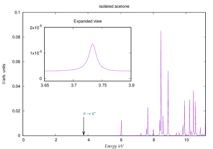
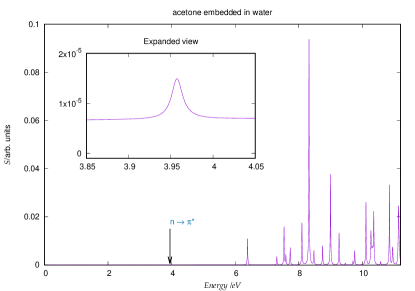
Figure 4: Absorption spectrum of isolated acetone (left panel) and embedded acetone in a water cluster (right panel)

It is worth noting that, due to its low intensity, this transition is particularly challenging for a real-time propagation framework. To obtain a spectrum up to 11 eV, we carried out a simulation consisting of $20000$ time steps and lasting 2000 a.u (48 fs). This relatively long simulation time demonstrates the numerical stability of the approach and its implementation.

	iso./eV	emb./eV	$\Delta E$/eV
Psi4-rt-PyEmbed	3.7337	3.9583	0.225
ADF-LR-FDE	3.7928	3.9749	0.182

Table 4: Isolated and embedded in a water cluster acetone $n\to\pi^{*}$ transition, reported for both ADF-LR-FDE and our Psi4-rt-PyEmbed code.

As an overall check of our implementation we compare the shift of the $n\to\pi^{*}$ transition observed between isolated and embedded in a water cluster acetone obtained using both our Psi4-rt-PyEmbed and the ADF-LR-FDE methods. The active system response was calculated at BLYP level of theory, while Thomas-Fermi and LDA functionals were employed for the non-additive kinetic and exchange-correlation terms respectively of the embedding potential in the ADF-LR-FDE calculation. As one can observe by looking at the values reported in Table 4, we obtain a good agreement in the absolute values, both isolated and embedded acetone, and the computed shift is likewise in rather good agreement.

4.4 FDE-rt-TDDFT in the non-linear regime

A specificity in the the real-time approach is that the evolution of the electron density can be driven by an real-valued electric field whose shape can be explicitly modulated. Realistic laser fields can be modeled by a sine function of $\omega_{0}$ frequency using any physically meaningful enveloping function. Using an explicit external field is a key tool in optical control theory, furthermore it is possible, employing high intensity field, to study phenomena beyond linear-response, i.e hyperpolarizability coefficients and high harmonic generation in molecules. The latter point will be detailed in the following section.

In this section we demonstrate that the uFDE-rt-TDDFT scheme gives stable numerical results not only in the perturbative regime, as shown above, but also in the presence of intense fields. Physically meaningful laser fields are adequately represented by sinusoidal pulse of the form $E(t)=f(t)\sin(\omega_{0}t)$ where $\omega_{0}$ is the carrier frequency. In this work we employ, a $\cos^{2}$ shape for the envelope function¹²⁶:

$$f(t)=E_{0}\cos^{2}\Big{(}\frac{\pi}{2\sigma}(\tau-t)\Big{)}\qquad for\quad|t-\tau|\leq\tau$$

$$0\qquad\text{elsewhere}$$

where $\tau$ is the width of the field envelope. We have calculated the response of H₂O embedded in a water cluster model made of five water molecules (all the details about the geometry have been reported in the previous section) to a $\cos^{2}$-shaped laser field with carrier frequency $\omega_{0}=$ 1.55 eV (analogously to a Ti:Sapphire laser), and intensity $I=1.02\times 10^{14}Wcm^{-2}$ (which corresponds to a field $E=0.054$ au) and a duration of 20 optical cycles. Each cycle lasts $2\pi/\omega_{0}$, and the overall pulse spans over 2250.0 au (i.e. 54 fs). The field has been chosen along the molecular symmetry axis ($z$) and the 6-311++G** basis set and B3LYP functional were used. The propagation was carried out for a total time of 3500 a.u without any numerical instabilities.

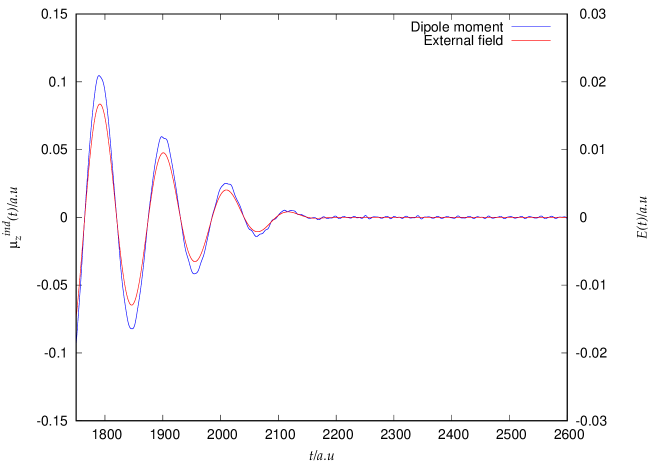
Figure 5: Induced dipole moment in H₂O molecule. The representation of the external field is also reported as a green line.

As shown in Fig. 5, the induced dipole does not follow the applied field adiabatically when a strong field is applied, especially in the few last optical cycles, strong diabatic effects are clearly present. These effects lead to the presence of a residual dipole oscillation. Following a previous work on high harmonic generation (HHG) in H₂ molecule, ¹²⁶ we extract the high-order harmonic intensities via the Fourier transform of the laser-driven induced dipole moment (neglecting the remaining part, i.e for $t$ larger than $\tau$, i.e 2250 au in the present simulation) as

$$P(\omega)\propto\Bigg{|}\int_{t_{1}}^{t_{2}}\mu_{z}(t)exp(-i\omega t)dt\Bigg{|}^{2}$$ (21)

In Fig. 6 we report the base-10 logarithm of the spectral intensity for the embedded water molecule and we compare it to the HHG of the isolated water calculated that has the same geometry it has in the cluster model. In the case of the isolated water molecule we are able to observe relatively well defined peaks up to the 21th harmonics. We mention that this finding qualitatively agrees with data obtained by Sun et al. ²⁰ (see Figure 3 of Ref.²⁰).

An important parameter in the analysis of the HHG spectrum is the value of the energy cutoff ($E_{cutoff}$), which is related with the maximum number of high harmonics ($N_{max}\approx E_{cutoff}/\omega_{0}$). In a semiclassical formulation ¹²⁷, which, among others assumes that only a single electron is active for HHG, $E_{cutoff}\approx I_{p}+3.17U_{p}$, where $I_{p}$ is the ionization potential of the system and $U_{p}$ ($U_{p}=\frac{E^{2}}{4\omega_{0}^{2}}$) is the ponderomotive energy in the laser field of strength $E$ and frequency $\omega_{0}$ ¹²⁷. In the case of molecular systems, the HHG spectra present more complex features and the above formula it is not strictly valid. With the laser parameters used here ($E=0.054$ a.u, $\omega_{0}=0.05696$ a.u.) and the experimental ionization potential of H${}_{2}O$ ($I_{p}=0.4637$ a.u.), the above formula predicts a $E_{cutoff}$ value of 1.17601 a.u. ($N_{max}$ at about the 21th harmonic), which is remarkably consistent with HHG spectra we observed here.

For the water molecule embedded in the cluster the same boundary can be approximately found corresponding to the 16th harmonic. The peaks at higher energies have a very small intensity and are much less resolved above the 16th harmonic. The flattening of the HHG intensity pattern is therefore solely due the introduction of the embedding potential of the surrounding cluster. The latter is consistent with a shift towards lower ionization energy passing from free water molecule to a small water cluster observed experimentally¹²⁸.

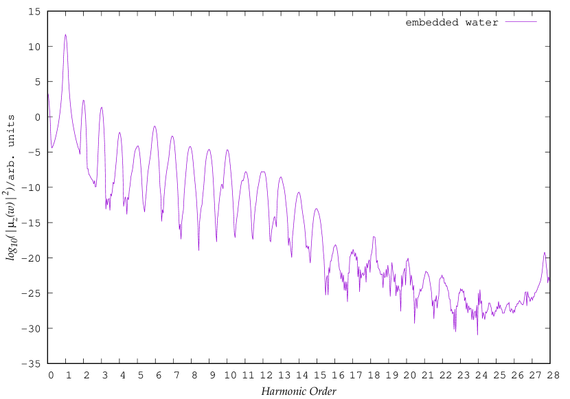
Figure 6: Upper panel: Emission spectrum of isolated water molecule. Lower panel: Emission spectrum of the same water molecule embedded in the (H₂O)₅ cluster

4.5 Computational constraints

Before concluding this work it may be interesting to put forward some assessments in terms of time statistics, to be used as a basis for optimizing the computation time and speed-up any uFDE-rt-TDDFT calculations. We are using a water-ammonia complex as a general test-case, where the geometry of the adduct has been taken from Ref.129 and the water is the active subsystem.

In the real-time framework the embedding potential is, evidently, an implicit time-dependent quantity. Since in the uncoupled FDE framework the density of the environment is kept frozen, the embedding potential depends on time only through the relatively small contributions given by the exchange-correlation and kinetic non-additive terms, which in turn it depends on time only through the density of the active subsystem. The electrostatic potential, due to the frozen electron density and nuclear charges of the environment, is the leading term in the overall potential. Thus, it may be reasonable to choose a longer time step for the update of the embedding potential, which is weakly varying in time.

In order to investigate such a possible speed-up, we carried out different simulations in which the time interval of the embedding potential updating is progressively increased. The results are reported in Table 5. Of course, as the number of time steps between consecutive updates is increased (i.e. the embedding potential is updated less often), the total time needed to perform the full simulation goes down, as the time spent in computing the embedding potential decreases. The update rate of the embedding potential during the propagation affects to some extent the position of the peaks in the absorption spectrum. As can be seen in Fig. 7 the different traces corresponding to dipole strength functions calculated with different update rates, do not differ significantly and tend to coalesce as the number of time steps between consecutive updates decreases below 30 time steps. In particular, in the case of the lowest-energy transition, the energy shift corresponding to a quite long update period (roughly 300 time steps) is of the order of 0.02 eV.

Table 5: Time in seconds as a function of the number n of time steps between consecutive updates of the embedding potential. ^f : time for V${}_{\text{emb}}$ evaluation. ^g : Total time for V${}_{\text{emb}}$ evaluation in the propagation. ^h : Total time needed for 100 real-time iterations

tf	tg	th	$n$
0.87	-	94.84	inf (static)
0.87	2.59	97.52	30
0.85	4.32	99.26	20
0.86	8.56	103.31	10
0.86	85.67	180.97	1

We also reported the partition between different tasks of the time needed for the calculation of the embedding potential in Table 6. As seen before, the calculation of the embedding potential is largely dominated by the projection to the basis set of the embedding potential from the numerical-grid representation. Therefore, some preliminary tests in reducing the number of grid points were carried out, and the results are presented in Fig. 8. It can be seen that there is no significant modification in the peak positions due to the use of a coarser integration grid: the overall spectrum is essentially stable and no artifacts are introduced.

Table 6: Time usage in seconds. ^a : Density on grid (through MOs). ^b : XCFun (non-additive potential calculation). ^c : V${}_{\text{emb}}$ projection onto the basis set ^d : Total time for V${}_{\text{emb}}$ evaluation.

ta	tb	tc	td
0.01	0.33	0.53	0.87

We furthermore note the possibility to use small grid localized solely on the active system by utilizing the fact that the embedding potential is projected on the localized basis set functions of the active system (see Eq.20), which makes it possible to neglect points on which these functions have a small value.

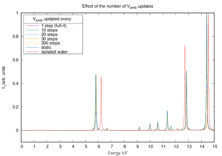
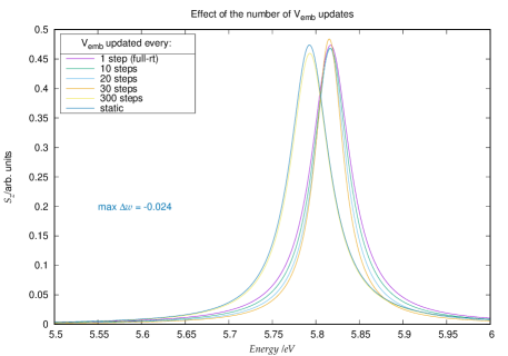
Figure 7: Left: Frequency shift in the S_z function due to increasing rate of update of the embedding potential. The peaks corresponding to the isolated water molecule are also reported as red trace. Right: Expanded view of the homo-lumo transition

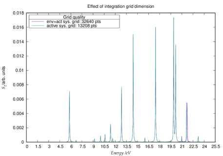
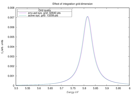
Figure 8: Comparison of $S_{z}$ dipole strength function obtained with two different integration grids. The violet trace corresponds to the full supramolecular integration grid, while the green trace to the active system grid. Right: Expanded view of the lowest-lying transition

5 Conclusions and perspectives

In this work we have focused on the implementation of the Frozen Density Embedding scheme in the real-time TDDFT. We have integrated the Psi4Numpy real-time module we recently developed within the PyADF framework. We have devised a real-time FDE scheme in which the active density is evolved under the presence of the embedding potential. This implementation relies on a multiscale approach, since the embedding potential is calculated by means of PyADF, while the propagation is carried out by Psi4Numpy. We tested the implementation on a simple water cluster showing that the time needed for the propagation scales linearly with the cluster size. We studied many low-lying transitions in the case of a water molecule embedded in ammonia, and we showed that the shift of excitation energies with respect to the isolated water molecule is in good agreement with the results obtained using linear response FDE TDDFT implemented in ADF. Finally, we tackled a challenging case for rt-TDDFT, by computing the lowest-energy transition of acetone, which features an extremely low intensity. The corresponding signal can be identified in the computed spectrum, and we evaluated the solvatochromic shift due to the presence of a surrounding water cluster. We obtained a frequency shift of 0.225 eV, close to the reference value, 0.182 eV, from LR-FDE TDDFT as implemented in ADF. The scheme we developed has proven to be reliable also in the case of propagation in the non-linear regime. As a demonstration, we perturbed with a strong electric field a water molecule surrounded by five water molecules acting as frozen environment. Numerically stable induced dipole moment and corresponding emission spectrum were obtained.

Finally, we like to state that the present work provides an excellent framework for future developments. It is for instance possible and desirable to optimize the embedding potential construction. In our implementation (i.e. Psi4-rt-PyEmbed) the projection onto the basis set of the embedding potential from the numerical grid representation dominates the computational burden. The change of the embedding potential matrix in time, (i.e the difference at two consecutive time steps) depends on the relatively small contributions given by the exchange-correlation and kinetic non-additive terms. Significant improvement could be achieved by exploiting the sparsity of the matrix corresponding to that difference. Moreover, the use of smaller integration grid would probably further improve the procedure. Last but not least, the effect of relaxation of the environment has to be investigated. In our uncoupled FDE-rt-TDDFT scheme we are able to study local transitions within a given subsystem, and particularly those of the active system under the influence of the embedding potential due to the frozen environment. Thus we neglect transitions involving the environment and those due to the couplings of the subsystems. Relaxing the environment can be crucial both in the linear-response framework, in order to recover supramolecular excitations, and in the non-linear regime where a polarizable environment could heavily affect the hyperpolarizabilities of the target system. The limit of the uncoupled FDE scheme can be overcome by carrying out a simultaneous propagation of subsystems ⁷⁰ and the computational framework developed in the present work represents an important step in that direction.

6 Acknowledgements

CRJ and ASPG acknowledge funding from the Franco-German project CompRIXS (Agence nationale de la recherche ANR-19-CE29-0019, Deutsche Forschungsgemeinschaft JA 2329/6-1). ASPG further acknowledges support from the CNRS Institute of Physics (INP), PIA ANR project CaPPA (ANR-11-LABX-0005-01), I-SITE ULNE project OVERSEE (ANR-16-IDEX-0004), the French Ministry of Higher Education and Research, region Hauts de France council and European Regional Development Fund (ERDF) project CPER CLIMIBIO. CRJ acknowledges funding from the Deutsche Forschungsgemeinschaft for the development of PyADF (Project Suresoft, JA 2329/7-1).

References

- Hardin et al. 2009 Hardin, B. E.; Hoke, E. T.; Armstrong, P. B.; Yum, J.-H.; Comte, P.; Torres, T.; Fréchet, J. M.; Nazeeruddin, M. K.; Grätzel, M.; McGehee, M. D. Increased light harvesting in dye-sensitized solar cells with energy relay dyes. Nature Photonics 2009, 3, 406
- Hagfeldt et al. 2010 Hagfeldt, A.; Boschloo, G.; Sun, L.; Kloo, L.; Pettersson, H. Dye-sensitized solar cells. Chem, Rev. 2010, 110, 6595–6663
- Salières et al. 1999 Salières, P.; Le Déroff, L.; Auguste, T.; Monot, P.; d’Oliveira, P.; Campo, D.; Hergott, J.-F.; Merdji, H.; Carré, B. Frequency-Domain Interferometry in the XUV with High-Order Harmonics. Phys. Rev. Lett. 1999, 83, 5483–5486
- Paul et al. 2001 Paul, P. M.; Toma, E. S.; Breger, P.; Mullot, G.; Augé, F.; Balcou, P.; Muller, H. G.; Agostini, P. Observation of a Train of Attosecond Pulses from High Harmonic Generation. Science 2001, 292, 1689–1692
- Bass et al. 1962 Bass, M.; Franken, P. A.; Ward, J. F.; Weinreich, G. Optical Rectification. Phys. Rev. Lett. 1962, 9, 446–448
- Kadlec et al. 2005 Kadlec, F.; Kužel, P.; Coutaz, J.-L. Study of terahertz radiation generated by optical rectification on thin gold films. Opt. Lett. 2005, 30, 1402–1404
- Keldysh 2017 Keldysh, L. V. Multiphoton ionization by a very short pulse. Physics-Uspekhi 2017, 60, 1187–1193
- Eberly et al. 1991 Eberly, J.; Javanainen, J.; Rzażewski, K. Above-threshold ionization. Physics Reports 1991, 204, 331 – 383
- Gallmann et al. 2012 Gallmann, L.; Cirelli, C.; Keller, U. Attosecond Science: Recent Highlights and Future Trends. Annual Review of Physical Chemistry 2012, 63, 447–469, PMID: 22404594
- Ramasesha et al. 2016 Ramasesha, K.; Leone, S. R.; Neumark, D. M. Real-Time Probing of Electron Dynamics Using Attosecond Time-Resolved Spectroscopy. Annual Review of Physical Chemistry 2016, 67, 41–63, PMID: 26980312
- Attar et al. 2017 Attar, A. R.; Bhattacherjee, A.; Pemmaraju, C. D.; Schnorr, K.; Closser, K. D.; Prendergast, D.; Leone, S. R. Femtosecond x-ray spectroscopy of an electrocyclic ring-opening reaction. Science 2017, 356, 54–59
- Wolf et al. 2019 Wolf, T. J. A.; Sanchez, D. M.; Yang, J.; Parrish, R. M.; Nunes, J. P. F.; Centurion, M.; Coffee, R.; Cryan, J. P.; Ghr, M.; Hegazy, K.; Kirrander, A.; Li, R. K.; Ruddock, J.; Shen, X.; Vecchione, T.; Weathersby, S. P.; Weber, P. M.; Wilkin, K.; Yong, H.; Zheng, Q.; Wang, X. J.; Minitti, M. P.; Martinez, T. J. The photochemical ring-opening of 1,3-cyclohexadiene imaged by ultrafast electron diffraction. Nat. Chem. 2019, 11, 504–509
- Ruddock et al. 2019 Ruddock, J. M.; Zotev, N.; Stankus, B.; Yong, H.; Bellshaw, D.; Boutet, S.; Lane, T. J.; Liang, M.; Carbajo, S.; Du, W.; Kirrander, A.; Minitti, M.; Weber, P. M. Simplicity Beneath Complexity: Counting Molecular Electrons Reveals Transients and Kinetics of Photodissociation Reactions. Angew. Chem. Int. Ed. 2019, 131, 6437–6441
- Kim et al. 2015 Kim, K. H.; Kim, J. G.; Nozawa, S.; Sato, T.; Oang, K. Y.; Kim, T. W.; Ki, H.; Jo, J.; Park, S.; Song, C.; Sato, T.; Ogawa, K.; Togashi, T.; Tono, K.; Yabashi, M.; Ishikawa, T.; Kim, J.; Ryoo, R.; Kim, J.; Ihee, H.; Adachi, S.-i. Direct observation of bond formation in solution with femtosecond X-ray scattering. Nature 2015, 518, 385–389
- Sharifi et al. 2007 Sharifi, M.; Kong, F.; Chin, S. L.; Mineo, H.; Dyakov, Y.; Mebel, A. M.; Chao, S. D.; Hayashi, M.; Lin, S. H. Experimental and Theoretical Investigation of High-Power Laser Ionization and Dissociation of Methane. J. Phys. Chem. A 2007, 111, 9405–9416
- Zigo et al. 2017 Zigo, S.; Le, A.-T.; Timilsina, P.; Trallero-Herrero, C. A. Ionization study of isomeric molecules in strong-field laser pulses. Scientific reports 2017, 7, 42149
- Goings et al. 2018 Goings, J. J.; Lestrange, P. J.; Li, X. Real-time time-dependent electronic structure theory. WIREs Computational Molecular Science 2018, 8, e1341
- Ekström et al. 2010 Ekström, U.; Visscher, L.; Bast, R.; Thorvaldsen, A. J.; Ruud, K. Arbitrary-Order Density Functional Response Theory from Automatic Differentiation. J. Chem. Theory Comput. 2010, 6, 1971–1980
- Rosa et al. 2019 Rosa, M.; Gil, G.; Corni, S.; Cammi, R. Quantum optimal control theory for solvated systems. J. Chem. Phys. 2019, 151, 194109
- Sun et al. 2007 Sun, J.; Song, J.; Zhao, Y.; Liang, W.-Z. Real-time propagation of the reduced one-electron density matrix in atom-centered Gaussian orbitals: Application to absorption spectra of silicon clusters. J. Chem. Phys. 2007, 127, 234107
- Li et al. 2005 Li, X.; Smith, S. M.; Markevitch, A. N.; Romanov, D. A.; Levis, R. J.; Schlegel, H. B. A time-dependent Hartree-Fock approach for studying the electronic optical response of molecules in intense fields. Phys. Chem. Chem. Phys. 2005, 7, 233–239
- Eshuis et al. 2008 Eshuis, H.; Balint-Kurti, G. G.; Manby, F. R. Dynamics of molecules in strong oscillating electric fields using time-dependent Hartree-Fock theory. J. Chem. Phys. 2008, 128, 114113
- Theilhaber 1992 Theilhaber, J. Ab initio simulations of sodium using time-dependent density-functional theory. Phys. Rev. B 1992, 46, 12990–13003
- Yabana and Bertsch 1996 Yabana, K.; Bertsch, G. F. Time-dependent local-density approximation in real time. Phys. Rev. B 1996, 54, 4484–4487
- Takimoto et al. 2007 Takimoto, Y.; Vila, F.; Rehr, J. Real-time time-dependent density functional theory approach for frequency-dependent nonlinear optical response in photonic molecules. J. Chem. Phys. 2007, 127, 154114
- Andrade et al. 2015 Andrade, X.; Strubbe, D.; De Giovannini, U.; Larsen, A. H.; Oliveira, M. J.; Alberdi-Rodriguez, J.; Varas, A.; Theophilou, I.; Helbig, N.; Verstraete, M. J.; Stella, L.; Nogueira, F.; Aspuru-Guzik, A.; Castro, A.; Marques, M. A. L.; Rubio, A. Real-space grids and the Octopus code as tools for the development of new simulation approaches for electronic systems. Phys. Chem. Chem. Phys. 2015, 17, 31371–31396
- Schleife et al. 2012 Schleife, A.; Draeger, E. W.; Kanai, Y.; Correa, A. A. Plane-wave pseudopotential implementation of explicit integrators for time-dependent Kohn-Sham equations in large-scale simulations. J. Chem. Phys. 2012, 137, 22A546
- Giannozzi et al. 2020 Giannozzi, P.; Baseggio, O.; Bonfà, P.; Brunato, D.; Car, R.; Carnimeo, I.; Cavazzoni, C.; de Gironcoli, S.; Delugas, P.; Ferrari Ruffino, F.; Ferretti, A.; Marzari, N.; Timrov, I.; Urru, A.; Baroni, S. Quantum ESPRESSO toward the exascale. J. Chem. Phys. 2020, 152, 154105
- Genova et al. 2017 Genova, A.; Ceresoli, D.; Krishtal, A.; Andreussi, O.; DiStasio Jr, R. A.; Pavanello, M. eQE: An open-source density functional embedding theory code for the condensed phase. Int. J. Quantum Chem. 2017, 117, e25401
- Liang et al. 2011 Liang, W.; Chapman, C. T.; Li, X. Efficient first-principles electronic dynamics. J. Chem. Phys. 2011, 134, 184102
- Morzan et al. 2014 Morzan, U. N.; Ramírez, F. F.; Oviedo, M. B.; Sánchez, C. G.; Scherlis, D. A.; Lebrero, M. C. G. Electron dynamics in complex environments with real-time time dependent density functional theory in a QM-MM framework. J. Chem. Phys. 2014, 140, 164105
- Lopata and Govind 2011 Lopata, K.; Govind, N. Modeling Fast Electron Dynamics with Real-Time Time-Dependent Density Functional Theory: Application to Small Molecules and Chromophores. J. Chem. Theory Comput. 2011, 7, 1344–1355
- Nguyen and Parkhill 2015 Nguyen, T. S.; Parkhill, J. Nonadiabatic Dynamics for Electrons at Second-Order: Real-Time TDDFT and OSCF2. J. Chem. Theory Comput. 2015, 11, 2918–2924
- Zhu and Herbert 2018 Zhu, Y.; Herbert, J. M. Self-consistent predictor/corrector algorithms for stable and efficient integration of the time-dependent Kohn-Sham equation. J. Chem. Phys. 2018, 148, 044117
- Repisky et al. 2015 Repisky, M.; Konecny, L.; Kadek, M.; Komorovsky, S.; Malkin, O. L.; Malkin, V. G.; Ruud, K. Excitation energies from real-time propagation of the four-component Dirac-Kohn-Sham equation. J. Chem. Theory Comput. 2015, 11, 980–991
- Goings et al. 2016 Goings, J. J.; Kasper, J. M.; Egidi, F.; Sun, S.; Li, X. Real time propagation of the exact two component time-dependent density functional theory. J. Chem. Phys. 2016, 145, 104107
- De Santis et al. 2020 De Santis, M.; Storchi, L.; Belpassi, L.; Quiney, H. M.; Tarantelli, F. PyBERTHART: A Relativistic Real-Time Four-Component TDDFT Implementation Using Prototyping Techniques Based on Python. J. Chem. Theory Comput. 2020, 16, 2410–2429
- 38 PyBertha project git URL: \urlhttps://github.com/lstorchi/pybertha written by: L. Storchi, M. De Santis, L. Belpassi
- Smith et al. 2018 Smith, D. G. A.; Burns, L. A.; Sirianni, D. A.; Nascimento, D. R.; Kumar, A.; James, A. M.; Schriber, J. B.; Zhang, T.; Zhang, B.; Abbott, A. S.; Berquist, E. J.; Lechner, M. H.; Cunha, L. A.; Heide, A. G.; Waldrop, J. M.; Takeshita, T. Y.; Alenaizan, A.; Neuhauser, D.; King, R. A.; Simmonett, A. C.; Turney, J. M.; Schaefer, H. F.; Evangelista, F. A.; DePrince, A. E.; Crawford, T. D.; Patkowski, K.; Sherrill, C. D. Psi4NumPy: An Interactive Quantum Chemistry Programming Environment for Reference Implementations and Rapid Development. J. Chem. Theory Comput. 2018, 14, 3504–3511
- Belpassi et al. 2011 Belpassi, L.; Storchi, L.; Quiney, H. M.; Tarantelli, F. Recent Advances and Perspectives in Four-Component Dirac-Kohn-Sham Calculations. Phys. Chem. Chem. Phys. 2011, 13, 12368–12394
- Belpassi et al. 2006 Belpassi, L.; Tarantelli, F.; Sgamellotti, A.; Quiney, H. M. Electron density fitting for the Coulomb problem in relativistic density-functional theory. The Journal of Chemical Physics 2006, 124, 124104
- Storchi et al. 2010 Storchi, L.; Belpassi, L.; Tarantelli, F.; Sgamellotti, A.; Quiney, H. M. An Efficient Parallel All-Electron Four-Component Dirac-Kohn-Sham Program Using a Distributed Matrix Approach. J. Chem. Theory Comput. 2010, 6, 384–394
- Belpassi et al. 2020 Belpassi, L.; De Santis, M.; Quiney, H. M.; Tarantelli, F.; Storchi, L. BERTHA: Implementation of a four-component Dirac-Kohn-Sham relativistic framework. The Journal of Chemical Physics 2020, 152, 164118
- Storchi et al. 2019 Storchi, L.; De Santis, M.; Belpassi, L. BERTHA and PyBERTHA: State of the Art for Full Four-Component Dirac-Kohn-Sham Calculations. Parallel Computing: Technology Trends, Proceedings of the International Conference on Parallel Computing, PARCO 2019, Prague, Czech Republic, September 10-13, 2019. 2019; pp 354–363
- Lopata et al. 2012 Lopata, K.; Van Kuiken, B. E.; Khalil, M.; Govind, N. Linear-Response and Real-Time Time-Dependent Density Functional Theory Studies of Core-Level Near-Edge X-Ray Absorption. J. Chem. Theory Comput. 2012, 8, 3284–3292
- Ding et al. 2013 Ding, F.; Van Kuiken, B. E.; Eichinger, B. E.; Li, X. An efficient method for calculating dynamical hyperpolarizabilities using real-time time-dependent density functional theory. J. Chem. Phys. 2013, 138, 064104
- Cheng et al. 2006 Cheng, C.-L.; Evans, J. S.; Van Voorhis, T. Simulating molecular conductance using real-time density functional theory. Phys. Rev. B 2006, 74, 155112
- Isborn and Li 2009 Isborn, C. M.; Li, X. Singlet-Triplet Transitions in Real-Time Time-Dependent Hartree-Fock/Density Functional Theory. J. Chem. Theory Comput. 2009, 5, 2415–2419
- Goings and Li 2016 Goings, J. J.; Li, X. An atomic orbital based real-time time-dependent density functional theory for computing electronic circular dichroism band spectra. J. Chem. Phys. 2016, 144, 234102
- Peralta et al. 2015 Peralta, J. E.; Hod, O.; Scuseria, G. E. Magnetization Dynamics from Time-Dependent Noncollinear Spin Density Functional Theory Calculations. J. Chem. Theory Comput. 2015, 11, 3661–3668
- Li et al. 2005 Li, X.; Tully, J. C.; Schlegel, H. B.; Frisch, M. J. Ab initio Ehrenfest dynamics. J. Chem. Phys. 2005, 123, 084106
- Kolesov et al. 2016 Kolesov, G.; Grånäs, O.; Hoyt, R.; Vinichenko, D.; Kaxiras, E. Real-Time TD-DFT with Classical Ion Dynamics: Methodology and Applications. J. Chem. Theory Comput. 2016, 12, 466–476
- Kadek et al. 2015 Kadek, M.; Konecny, L.; Gao, B.; Repisky, M.; Ruud, K. X-ray absorption resonances near L2,3-edges from real-time propagation of the Dirac-Kohn-Sham density matrix. Phys. Chem. Chem. Phys. 2015, 17, 22566–22570
- Konecny et al. 2016 Konecny, L.; Kadek, M.; Komorovsky, S.; Malkina, O. L.; Ruud, K.; Repisky, M. Acceleration of Relativistic Electron Dynamics by Means of X2C Transformation: Application to the Calculation of Nonlinear Optical Properties. J. Chem. Theory Comput. 2016, 12, 5823–5833
- Konecny et al. 2018 Konecny, L.; Kadek, M.; Komorovsky, S.; Ruud, K.; Repisky, M. Resolution-of-identity accelerated relativistic two- and four-component electron dynamics approach to chiroptical spectroscopies. J. Chem. Phys. 2018, 149, 204104
- Marques et al. 2003 Marques, M. A. L.; López, X.; Varsano, D.; Castro, A.; Rubio, A. Time-Dependent Density-Functional Approach for Biological Chromophores: The Case of the Green Fluorescent Protein. Phys. Rev. Lett. 2003, 90, 258101
- Liang et al. 2012 Liang, W.; Chapman, C. T.; Ding, F.; Li, X. Modeling Ultrafast Solvated Electronic Dynamics Using Time-Dependent Density Functional Theory and Polarizable Continuum Model. J. Phys. Chem. A 2012, 116, 1884–1890
- Nguyen et al. 2012 Nguyen, P. D.; Ding, F.; Fischer, S. A.; Liang, W.; Li, X. Solvated First-Principles Excited-State Charge-Transfer Dynamics with Time-Dependent Polarizable Continuum Model and Solvent Dielectric Relaxation. J. Phys. Chem. Lett. 2012, 3, 2898–2904
- Pipolo et al. 2014 Pipolo, S.; Corni, S.; Cammi, R. The cavity electromagnetic field within the polarizable continuum model of solvation: An application to the real-time time dependent density functional theory. Computational and Theoretical Chemistry 2014, 1040-1041, 112 – 119, Excited states: From isolated molecules to complex environments
- Corni et al. 2015 Corni, S.; Pipolo, S.; Cammi, R. Equation of Motion for the Solvent Polarization Apparent Charges in the Polarizable Continuum Model: Application to Real-Time TDDFT. J. Phys. Chem. A 2015, 119, 5405–5416
- Ding et al. 2015 Ding, F.; Lingerfelt, D. B.; Mennucci, B.; Li, X. Time-dependent non-equilibrium dielectric response in QM/continuum approaches. J. Chem. Phys. 2015, 142, 034120
- Donati et al. 2017 Donati, G.; Wildman, A.; Caprasecca, S.; Lingerfelt, D. B.; Lipparini, F.; Mennucci, B.; Li, X. Coupling Real-Time Time-Dependent Density Functional Theory with Polarizable Force Field. J. Phys. Chem. Lett. 2017, 8, 5283–5289
- Wu et al. 2017 Wu, X.; Teuler, J.-M.; Cailliez, F.; Clavaguéra, C.; Salahub, D. R.; de la Lande, A. Simulating Electron Dynamics in Polarizable Environments. J. Chem. Theory Comput. 2017, 13, 3985–4002
- Gil et al. 2019 Gil, G.; Pipolo, S.; Delgado, A.; Rozzi, C. A.; Corni, S. Nonequilibrium Solvent Polarization Effects in Real-Time Electronic Dynamics of Solute Molecules Subject to Time-Dependent Electric Fields: A New Feature of the Polarizable Continuum Model. J. Chem. Theory Comput. 2019, 15, 2306–2319
- Koh et al. 2017 Koh, K. J.; Nguyen-Beck, T. S.; Parkhill, J. Accelerating Realtime TDDFT with Block-Orthogonalized Manby-Miller Embedding Theory. J. Chem. Theory Comput. 2017, 13, 4173–4178
- Lee et al. 2019 Lee, S. J. R.; Welborn, M.; Manby, F. R.; Miller, T. F. Projection-Based Wavefunction-in-DFT Embedding. Acc. Chem. Res. 2019, 52, 1359–1368
- Gomes and Jacob 2012 Gomes, A. S. P.; Jacob, Ch. R. Quantum-chemical embedding methods for treating local electronic excitations in complex chemical systems. Annu. Rep. Prog. Chem., Sect. C 2012, 108, 222
- Jacob and Neugebauer 2014 Jacob, Ch. R.; Neugebauer, J. Subsystem density-functional theory. WIREs Comput. Mol. Sci. 2014, 4, 325–362
- Wesolowski et al. 2015 Wesolowski, T. A.; Shedge, S.; Zhou, X. Frozen-Density Embedding Strategy for Multilevel Simulations of Electronic Structure. Chem. Rev. 2015, 115, 5891–5928
- Krishtal et al. 2015 Krishtal, A.; Ceresoli, D.; Pavanello, M. Subsystem real-time time dependent density functional theory. J. Chem. Phys. 2015, 142, 154116
- Wesolowski and Warshel 1993 Wesolowski, T. A.; Warshel, A. Frozen density functional approach for ab initio calculations of solvated molecules. J. Phys. Chem. 1993, 97, 8050–8053
- Senatore and Subbaswamy 1986 Senatore, G.; Subbaswamy, K. R. Density dependence of the dielectric constant of rare-gas crystals. Phys. Rev. B 1986, 34, 5754–5757
- Cortona 1992 Cortona, P. Direct determination of self-consistent total energies and charge densities of solids: A study of the cohesive properties of the alkali halides. Phys. Rev. B 1992, 46, 2008–2014
- Iannuzzi et al. 2006 Iannuzzi, M.; Kirchner, B.; Hutter, J. Density functional embedding for molecular systems. Chem. Phys. Lett. 2006, 421, 16 – 20
- Jacob et al. 2008 Jacob, C. R.; Neugebauer, J.; Visscher, L. A flexible implementation of frozen-density embedding for use in multilevel simulations. J. Comput. Chem. 2008, 29, 1011–1018
- Casida and Wesolowski 2004 Casida, M. E.; Wesolowski, T. A. Generalization of the Kohn-Sham equations with constrained electron density formalism and its time-dependent response theory formulation. Int. J. Quantum Chem. 2004, 96, 577–588
- Neugebauer 2007 Neugebauer, J. Couplings between electronic transitions in a subsystem formulation of time-dependent density functional theory. J. Chem. Phys. 2007, 126, 134116
- Neugebauer 2009 Neugebauer, J. On the calculation of general response properties in subsystem density functional theory. J. Chem. Phys. 2009, 131, 084104
- Tölle et al. 2019 Tölle, J.; Böckers, M.; Neugebauer, J. Exact subsystem time-dependent density-functional theory. J. Chem. Phys. 2019, 150, 181101
- Tölle et al. 2019 Tölle, J.; Böckers, M.; Niemeyer, N.; Neugebauer, J. Inter-subsystem charge-transfer excitations in exact subsystem time-dependent density-functional theory. J. Chem. Phys. 2019, 151, 174109
- Fux et al. 2010 Fux, S.; Jacob, C. R.; Neugebauer, J.; Visscher, L.; Reiher, M. Accurate frozen-density embedding potentials as a first step towards a subsystem description of covalent bonds. J. Chem. Phys. 2010, 132, 164101
- Goodpaster et al. 2010 Goodpaster, J. D.; Ananth, N.; Manby, F. R.; Miller, T. F. Exact nonadditive kinetic potentials for embedded density functional theory. J. Chem. Phys. 2010, 133, 084103
- Goodpaster et al. 2011 Goodpaster, J. D.; Barnes, T. A.; Miller, T. F. Embedded density functional theory for covalently bonded and strongly interacting subsystems. J. Chem. Phys. 2011, 134, 164108
- Huang et al. 2011 Huang, C.; Pavone, M.; Carter, E. A. Quantum mechanical embedding theory based on a unique embedding potential. J. Chem. Phys. 2011, 134, 154110
- Nafziger et al. 2011 Nafziger, J.; Wu, Q.; Wasserman, A. Molecular binding energies from partition density functional theory. J. Chem. Phys. 2011, 135, 234101
- Jacob et al. 2011 Jacob, C. R.; Beyhan, S. M.; Bulo, R. E.; Gomes, A. S. P.; Götz, A. W.; Kiewisch, K.; Sikkema, J.; Visscher, L. PyADF – A scripting framework for multiscale quantum chemistry. J. Comput. Chem. 2011, 32, 2328–2338
- Ekström 2019 Ekström, U. XCFun: Exchange-Correlation functionals with arbitrary order derivatives. \url https://github.com/dftlibs/xcfun, 2019
- Thomas 1927 Thomas, L. H. The calculation of atomic fields. Mathematical Proceedings of the Cambridge Philosophical Society 1927, 23, 542–548
- Lembarki and Chermette 1994 Lembarki, A.; Chermette, H. Obtaining a gradient-corrected kinetic-energy functional from the Perdew-Wang exchange functional. Phys. Rev. A 1994, 50, 5328–5331
- Mi and Pavanello 2020 Mi, W.; Pavanello, M. Nonlocal Subsystem Density Functional Theory. J. Phys. Chem. Lett. 2020, 11, 272–279
- Gomes et al. 2008 Gomes, A. S. P.; Jacob, C. R.; Visscher, L. Calculation of local excitations in large systems by embedding wave-function theory in density-functional theory. Phys. Chem. Chem. Phys. 2008, 10, 5353–5362
- Bouchafra et al. 2018 Bouchafra, Y.; Shee, A.; Réal, F.; Vallet, V.; Gomes, A. S. P. Predictive simulations of ionization energies of solvated halide ions with relativistic embedded Equation of Motion Coupled Cluster Theory. Phys. Rev. Lett. 2018, 121, 266001
- Halbert et al. 2019 Halbert, L.; Olejniczak, M.; Vallet, V.; Gomes, A. S. P. Investigating solvent effects on the magnetic properties of molybdate ions (MoO) with relativistic embedding. Int. J. Quantum Chem. 2019,
- Höfener et al. 2012 Höfener, S.; Severo Pereira Gomes, A.; Visscher, L. Molecular properties via a subsystem density functional theory formulation: A common framework for electronic embedding. J. Chem. Phys. 2012, 136, 044104
- Olejniczak et al. 2017 Olejniczak, M.; Bast, R.; Gomes, A. S. P. On the calculation of second-order magnetic properties using subsystem approaches in a relativistic framework. Phys. Chem. Chem. Phys. 2017, 19, 8400–8415
- Neugebauer et al. 2005 Neugebauer, J.; Jacob, C. R.; Wesolowski, T. A.; Baerends, E. J. An Explicit Quantum Chemical Method for Modeling Large Solvation Shells Applied to Aminocoumarin C151. J. Phys. Chem. A 2005, 109, 7805–7814
- Bulo et al. 2008 Bulo, R. E.; Jacob, C. R.; Visscher, L. NMR Solvent Shifts of Acetonitrile from Frozen Density Embedding Calculations. The Journal of Physical Chemistry A 2008, 112, 2640–2647
- Castro et al. 2004 Castro, A.; Marques, M. A. L.; Rubio, A. Propagators for the time-dependent Kohni-Sham equations. J. Chem. Phys. 2004, 121, 3425–3433
- Meng and Kaxiras 2008 Meng, S.; Kaxiras, E. Real-time, local basis-set implementation of time-dependent density functional theory for excited state dynamics simulations. J. Chem. Phys. 2008, 129, 054110
- Press et al. 2007 Press, W. H.; Teukolsky, S. A.; Vetterling, W. T.; Flannery, B. P. Numerical recipes 3rd edition: The art of scientific computing; Cambridge university press, 2007
- Magnus 1954 Magnus, W. On the exponential solution of differential equations for a linear operator. Communications on Pure and Applied Mathematics 1954, 7, 649–673
- Casas and Iserles 2006 Casas, F.; Iserles, A. Explicit Magnus expansions for nonlinear equations. Journal of Physics A: Mathematical and General 2006, 39, 5445–5461
- Zhu and Herbert 2018 Zhu, Y.; Herbert, J. M. Self-consistent predictor/corrector algorithms for stable and efficient integration of the time-dependent Kohn-Sham equation. J. Chem. Phys. 2018, 148, 044117
- Bandrauk et al. 2009 Bandrauk, A. D.; Chelkowski, S.; Diestler, D. J.; Manz, J.; Yuan, K.-J. Quantum simulation of high-order harmonic spectra of the hydrogen atom. Phys. Rev. A 2009, 79, 023403
- Jacob et al. 2020 Jacob, Ch. R.; Beyhan, S. M.; Bulo, R. E.; Gomes, A. S. P.; Goetz, A.; Handzlik, M.; Kiewisch, K.; Klammler, M.; Sikkema, J.; Visscher, L. PyADF — A Scripting Framework for Multiscale Quantum Chemistry: Version 0.96. 2020; URL: https://github.com/chjacob-tubs/pyadf-releases, DOI: 10.5281/zenodo.3834283
- Gomes and Jacob 2020 Gomes, A. S. P.; Jacob, Ch. R. PyEmbed — A Frozen-Density Embedding Module for PyADF. 2020; available at DOI: 10.5281/zenodo.3834283
- Schmitt-Monreal and Jacob 2020 Schmitt-Monreal, D.; Jacob, Ch. R. Frozen-density embedding-based many-body expansions. Int. J. Quantum Chem. 2020, n/a, e26228, in press, DOI: 10.1002/qua.26228
- 108 M. De Santis, git URL: \urlhttps://github.com/lstorchi/pybertha/tree/master/psi4embedrt within the PyBertha project: \urlhttps://github.com/lstorchi/pybertha written by: L. Storchi, M. De Santis, L. Belpassi
- De Santis 2020 De Santis, M. Numerical data and post-processing material. 2020; available at: DOI: 10.5281/zenodo.3885610
- Parrish et al. 2017 Parrish, R. M.; Burns, L. A.; Smith, D. G. A.; Simmonett, A. C.; DePrince, A. E.; Hohenstein, E. G.; Bozkaya, U.; Sokolov, A. Y.; Di Remigio, R.; Richard, R. M.; Gonthier, J. F.; James, A. M.; McAlexander, H. R.; Kumar, A.; Saitow, M.; Wang, X.; Pritchard, B. P.; Verma, P.; Schaefer, H. F.; Patkowski, K.; King, R. A.; Valeev, E. F.; Evangelista, F. A.; Turney, J. M.; Crawford, T. D.; Sherrill, C. D. Psi4 1.1: An Open-Source Electronic Structure Program Emphasizing Automation, Advanced Libraries, and Interoperability. J. Chem. Theory Comput. 2017, 13, 3185–3197
- Storchi 2020 Storchi, L. Python 3 port of PyADF v0.96. 2020; DOI: 10.5281/zenodo.3834286
- Storchi 2020 Storchi, L. Python 3 port of XcFun a486a3f148. 2020; URL: https://github.com/lstorchi/xcfun
- 113 Baerends, E. J.; Ziegler, T.; Atkins, A. J.; Autschbach, J.; Bashford, D.; Baseggio, O.; Bérces, A.; Bickelhaupt, F. M.; Bo, C.; Boerritger, P. M.; Cavallo, L.; Daul, C.; Chong, D. P.; Chulhai, D. V.; Deng, L.; Dickson, R. M.; Dieterich, J. M.; Ellis, D. E.; van Faassen, M.; Ghysels, A.; Giammona, A.; van Gisbergen, S. J. A.; Goez, A.; Götz, A. W.; Gusarov, S.; Harris, F. E.; van den Hoek, P.; Hu, Z.; Jacob, C. R.; Jacobsen, H.; Jensen, L.; Joubert, L.; Kaminski, J. W.; van Kessel, G.; König, C.; Kootstra, F.; Kovalenko, A.; Krykunov, M.; van Lenthe, E.; McCormack, D. A.; Michalak, A.; Mitoraj, M.; Morton, S. M.; Neugebauer, J.; Nicu, V. P.; Noodleman, L.; Osinga, V. P.; Patchkovskii, S.; Pavanello, M.; Peeples, C. A.; Philipsen, P. H. T.; Post, D.; Pye, C. C.; Ramanantoanina, H.; Ramos, P.; Ravenek, W.; Rodríguez, J. I.; Ros, P.; Rüger, R.; Schipper, P. R. T.; Schlüns, D.; van Schoot, H.; Schreckenbach, G.; Seldenthuis, J. S.; Seth, M.; Snijders, J. G.; Solà, M.; M., S.; Swart, M.; Swerhone, D.; te Velde, G.; Tognetti, V.; Vernooijs, P.; Versluis, L.; Visscher, L.; Visser, O.; Wang, F.; Wesolowski, T. A.; van Wezenbeek, E. M.; Wiesenekker, G.; Wolff, S. K.; Woo, T. K.; Yakovlev, A. L. ADF2017, SCM, Theoretical Chemistry, Vrije Universiteit, Amsterdam, The Netherlands, https://www.scm.com
- Dułak et al. 2009 Dułak, M.; Kamiński, J. W.; Wesolowski, T. A. Linearized orbital-free embedding potential in self-consistent calculations. Int. J. Quantum Chem. 2009, 109, 1886–1897
- Wesolowski 2004 Wesolowski, T. A. Hydrogen-Bonding-Induced Shifts of the Excitation Energies in Nucleic Acid Bases: An Interplay between Electrostatic and Electron Density Overlap Effects. J. Am. Chem. Soc. 2004, 126, 11444–11445
- Te Velde et al. 2001 Te Velde, G. t.; Bickelhaupt, F. M.; Baerends, E. J.; Fonseca Guerra, C.; van Gisbergen, S. J.; Snijders, J. G.; Ziegler, T. Chemistry with ADF. J. Comput. Chem. 2001, 22, 931–967
- Bruner et al. 2016 Bruner, A.; LaMaster, D.; Lopata, K. Accelerated broadband spectra using transition dipole decomposition and Padé approximants. J. Chem. Theory Comput. 2016, 12, 3741–3750
- Dunning 1989 Dunning, T. H. Gaussian basis sets for use in correlated molecular calculations. I. The atoms boron through neon and hydrogen. J. Chem. Phys. 1989, 90, 1007–1023
- Kendall et al. 1992 Kendall, R. A.; Dunning, T. H.; Harrison, R. J. Electron affinities of the first-row atoms revisited. Systematic basis sets and wave functions. J. Chem. Phys. 1992, 96, 6796–6806
- Becke 1988 Becke, A. D. Density-functional exchange-energy approximation with correct asymptotic behavior. Phys. Rev. A 1988, 38, 3098–3100
- Lee et al. 1988 Lee, C.; Yang, W.; Parr, R. G. Development of the Colle-Salvetti correlation-energy formula into a functional of the electron density. Phys. Rev. B 1988, 37, 785–789
- Vosko et al. 1980 Vosko, S. H.; Wilk, L.; Nusair, M. Accurate spin-dependent electron liquid correlation energies for local spin density calculations: a critical analysis. Canadian Journal of Physics 1980, 58, 1200–1211
- Slater 1951 Slater, J. C. A Simplification of the Hartree-Fock Method. Phys. Rev. 1951, 81, 385–390
- Jacob et al. 2006 Jacob, C. R.; Neugebauer, J.; Jensen, L.; Visscher, L. Comparison of frozen-density embedding and discrete reaction field solvent models for molecular properties. Phys. Chem. Chem. Phys. 2006, 8, 2349–2359
- Höfener et al. 2013 Höfener, S.; Gomes, A. S. P.; Visscher, L. Solvatochromic shifts from coupled-cluster theory embedded in density functional theory. J. Chem. Phys. 2013, 139, 104106
- Luppi and Head-Gordon 2012 Luppi, E.; Head-Gordon, M. Computation of high-harmonic generation spectra of H2 And N2 in intense laser pulses using quantum chemistry methods and time-dependent density functional theory. Mol. Phys. 2012, 110, 909–923
- Lewenstein et al. 1994 Lewenstein, M.; Balcou, P.; Ivanov, M. Y.; L’Huillier, A.; Corkum, P. B. Theory of high-harmonic generation by low-frequency laser fields. Phys. Rev. A 1994, 49, 2117–2132
- Barth et al. 2009 Barth, S.; Oncak, M.; Ulrich, V.; Mucke, M.; Lischke, T.; Slavicek, P.; Hergenhahn, U. Valence Ionization of Water Clusters: From Isolated Molecules to Bulk. J. Phys. Chem. A 2009, 113, 13519–13527
- Klahr et al. 2018 Klahr, K.; Schlüns, D.; Neugebauer, J. Geometry Optimizations in a Subsystem Density Functional Theory Formalism: A Benchmark Study. J. Chem. Theory Comput. 2018, 14, 5631–5644