Reviving non-Minimal Horndeski-like Theories after GW170817: Kinetic Coupling Corrected Einstein-Gauss-Bonnet Inflation

Abstract

After the recent GW170817 event of the two neutron stars merging, many string corrected cosmological theories confronted the non-viability peril. This was due to the fact that most of these theories produce massive gravitons primordially. Among these theories were the ones containing a non-minimal kinetic coupling correction term in the Lagrangian. In this work we demonstrate how these theories may be revived and we show how these theories can produce primordial gravitational waves with speed $c_{T}^{2}=1$ in natural units, thus complying with the GW170817 event. As we show, if the gravitational action of an Einstein-Gauss-Bonnet theory also contains a kinetic coupling of the form $\sim\xi(\phi)G^{\mu\nu}\partial_{\mu}\phi\partial_{\nu}\phi$, the condition of having primordial massless gravitons, or equivalently primordial gravitational waves with speed $c_{T}^{2}=1$ in natural units, results to certain conditions on the scalar field dependent coupling function of the Gauss-Bonnet term, which is also the non-minimal coupling of the kinetic coupling. We extensively study the phenomenological implications of such a theory focusing on the inflationary era, by only assuming slow-roll dynamics for the scalar field. Accordingly, we briefly study the case that the scalar field evolves in a constant-roll way. By using some illustrative examples, we demonstrate that the viability of the theoretical framework at hand may easily be achieved. Also, theories containing terms of the form $\sim\xi(\phi)\Box\phi g^{\mu\nu}\partial_{\mu}\phi\partial_{\nu}\phi$ and $\sim\xi(\phi)\left(g^{\mu\nu}\partial_{\mu}\phi\partial_{\nu}\phi\right)^{2}$ are also lead to the same gravitational wave speed as the theory we shall study in this paper, so this covers a larger class of Horndeski theories.

I Introduction

The primordial Universe is one of the mysteries that modern theoretical cosmologists and physicists are trying to understand. Our approach to the primordial Universe is through a regime of classical gravity towards to the unknown era of quantum gravity or the “theory of everything” which is believed to govern the small scale physics and unifies all forces in nature. In between the classical gravity regime and the quantum gravity regime, theoretical cosmologists believe that an era of abrupt acceleration occurred, known as inflationary era. This era is at the border of classical and quantum gravity, so many believe that it should have some imprints of the quantum gravity era, in the effective theory that controls the inflationary regime. The most appealing theoretical proposal for the “theory of everything” is nowadays string theory in all its different forms. If string theory controls the quantum gravity era, it is reasonable to expect that the effective theory that controls the inflationary era might have terms which originate in the complete M-theory Lagrangian. In some sense the classical inflationary theory should contain several string theory corrections. A particularly appealing class of theories which contains string theory motivated corrections is Einstein-Gauss-Bonnet theory of gravity Hwang:2005hb ; Nojiri:2006je ; Cognola:2006sp ; Nojiri:2005vv ; Nojiri:2005jg ; Satoh:2007gn ; Bamba:2014zoa ; Yi:2018gse ; Guo:2009uk ; Guo:2010jr ; Jiang:2013gza ; Kanti:2015pda ; vandeBruck:2017voa ; Kanti:1998jd ; Kawai:1999pw ; Nozari:2017rta ; Chakraborty:2018scm ; Odintsov:2018zhw ; Kawai:1998ab ; Yi:2018dhl ; vandeBruck:2016xvt ; Kleihaus:2019rbg ; Bakopoulos:2019tvc ; Maeda:2011zn ; Bakopoulos:2020dfg ; Ai:2020peo ; Easther:1996yd ; Antoniadis:1993jc ; Antoniadis:1990uu ; Odintsov:2020sqy ; Odintsov:2020zkl ; Odintsov:2019clh . These theories, along with several extensions containing kinetic coupling corrections Hwang:2005hb are known to provide a viable inflationary era which can in many cases be compatible with the observational data, see Refs. Hwang:2005hb ; Nojiri:2006je ; Cognola:2006sp ; Nojiri:2005vv ; Nojiri:2005jg ; Satoh:2007gn ; Bamba:2014zoa ; Yi:2018gse ; Guo:2009uk ; Guo:2010jr ; Jiang:2013gza ; Kanti:2015pda ; vandeBruck:2017voa ; Kanti:1998jd ; Kawai:1999pw ; Nozari:2017rta ; Chakraborty:2018scm ; Odintsov:2018zhw ; Kawai:1998ab ; Yi:2018dhl ; vandeBruck:2016xvt ; Kleihaus:2019rbg ; Bakopoulos:2019tvc ; Maeda:2011zn ; Bakopoulos:2020dfg ; Ai:2020peo ; Easther:1996yd ; Antoniadis:1993jc ; Antoniadis:1990uu ; Odintsov:2020sqy ; Odintsov:2020zkl ; Odintsov:2019clh and references therein for details.

However, Einstein-Gauss-Bonnet theories have a serious flaw, namely the predict a non-zero graviton mass during the primordial inflationary era. This was not a problem until recently, the GW170817 event utterly changed the scenery in modern theoretical cosmology, excluding many modified gravity theories from being viable descriptions of the Universe, see Ref. Ezquiaga:2017ekz for a detailed account on this topic. This is because the two neutron stars merging event GW170817 GBM:2017lvd indicated that the gravitational waves arrived almost simultaneously with the gamma rays emitted from the neutron stars merging. Correspondingly, this observation clearly shows that the gravitational wave speed $c_{T}$ is nearly equal to unity, that is $c_{T}^{2}=1$ in natural units, which is equal to the speed of light. Thus theories that do not predict a massless graviton should no longer be considered as successful description of our Universe at large or small scales. It is remarkable though that many modified gravity theories Nojiri:2017ncd ; Nojiri:2010wj ; Nojiri:2006ri ; Capozziello:2011et ; Capozziello:2010zz ; delaCruzDombriz:2012xy ; Olmo:2011uz , still remain compatible with the observations, like $f(R)$ gravity or Gauss-Bonnet theories.

Now the question is, why an event that is observed at small redshifts should affect so seriously theories that predict a primordial massive graviton? The answer to this question is simple, there is no reason for the graviton to change its mass during the evolution of the Universe. So the answer to the above question, can also be cast in a question, why should the graviton mass during the inflationary era be different from the gravitons emitted from low redshift astrophysical sources? No particle physics process can explain why the graviton should have different mass during inflation, the post-inflationary era and at present time, at least to our knowledge.

In view of this way of thinking, in a previous work we studied how Einstein-Gauss-Bonnet theories can be compatible to the GW170817 event, and produce primordial gravitational waves with speed equal to that of light Odintsov:2020sqy ; Odintsov:2020zkl ; Odintsov:2019clh . As we showed, the condition $c_{T}^{2}=1$ restricts significantly the functional forms of the Gauss-Bonnet scalar coupling function $\xi(\phi)$ and the scalar potential. We also demonstrated that the GW170817-compatible theories can produce a viable inflationary era, compatible with the latest Planck data Akrami:2018odb .

In this work, we extend the study performed in our previous work Odintsov:2020sqy ; Odintsov:2020zkl ; Odintsov:2019clh , including in the effective action of Einstein-Gauss-Bonnet theories non-minimal kinetic coupling terms of the form $\sim\xi(\phi)G^{\mu\nu}\partial_{\mu}\phi\partial_{\nu}\phi$. These type of theories belong to the more general class of Horndeski theories horndeskioriginal ; Kobayashi:2019hrl ; Kobayashi:2016xpl ; Crisostomi:2016tcp ; Bellini:2015xja ; Gleyzes:2014qga ; Lin:2014jga ; Deffayet:2013lga ; Bettoni:2013diz ; Koyama:2013paa ; Starobinsky:2016kua ; Capozziello:2018gms ; BenAchour:2016fzp ; Starobinsky:2019xdp , and are also known as kinetic coupling theories Sushkov:2009hk ; Minamitsuji:2013ura ; Saridakis:2010mf ; Barreira:2013jma ; Sushkov:2012za ; Barreira:2012kk ; Skugoreva:2013ooa ; Gubitosi:2011sg ; Matsumoto:2015hua ; Deffayet:2010qz ; Granda:2010hb ; Matsumoto:2017gnx ; Gao:2010vr ; Granda:2009fh ; Germani:2010gm ; Fu:2019ttf and after the GW170817 event, these theories were significantly looked down upon, due to the fact that Horndeski theories produce primordial gravitational waves with speed less than that of light. Actually, Horndeski theories in view of GW170817 were also studied and discussed in Refs. Dima:2017pwp ; Kreisch:2017uet ; Arai:2017hxj . In this paper, we shall revive in a concrete way the Horndeski theories containing kinetic couplings of the form $\sim\xi(\phi)G^{\mu\nu}\partial_{\mu}\phi\partial_{\nu}\phi$, by imposing the constraint that the gravitational wave speed is equal to that of light. As we show in detail, the constraint $c_{T}^{2}=1$ results to a differential equation that determines uniquely the dynamical evolution of the scalar field. In addition, the coupling function $\xi(\phi)$ and the scalar potential are not freely chosen, but must satisfy a specific differential equation. Then by assuming that the slow-roll conditions hold true, we show that the inflationary phenomenology of GW170817-compatible kinetic coupling corrected Einstein-Gauss-Bonnet theory can be compatible with the latest Planck data Akrami:2018odb . We also perform the study in the case of a constant-roll evolution for the scalar field, and we show that the viability can be achieved in this case of dynamical evolution too. Finally, as we show, the same constraint that renders the kinetic coupling corrected Einstein-Gauss-Bonnet theories compatible with the GW170817 event, also renders theories containing terms $\sim\xi(\phi)\Box\phi g^{\mu\nu}\partial_{\mu}\phi\partial_{\nu}\phi$ and $\sim\xi(\phi)\left(g^{\mu\nu}\partial_{\mu}\phi\partial_{\nu}\phi\right)^{2}$ also compatible with the GW170817 event. Thus a broader class of Horndeski theories can be revived, however we restrict ourselves to the simplest case of having only kinetic coupling terms, because the extended theories are quite more difficult to study with regard to their inflationary phenomenology.

II Non-minimal Kinetic Coupling Corrected Einstein-Gauss-Bonnet Inflationary Phenomenology: Essential Features and Compatibility with GW170817 Constraints

In principle, Einstein-Gauss-Bonnet gravity is simply a string corrected scalar field theory with minimal coupling, thus a natural extension of this string corrected theory can be obtained by simply adding a non-minimal kinetic coupling, or other higher order string corrections containing derivatives of the scalar field, see Hwang:2005hb for more details on all the possible string corrections. In this work we shall assume that the gravitational action of a minimally coupled scalar field contains two string corrections, namely a Gauss-Bonnet term with a scalar field dependent coupling and a non-minimal kinetic coupling term, and the action has the following form,

$$\centering\mathcal{S}=\int{d^{4}x\sqrt{-g}\left(\frac{R}{2\kappa^{2}}-\frac{\omega}{2}g^{\mu\nu}\partial_{\mu}\phi\partial_{\nu}\phi-V(\phi)-\xi(\phi)\mathcal{G}-c\xi(\phi)G^{\mu\nu}\partial_{\mu}\phi\partial_{\nu}\phi\right)}\,,\@add@centering$$ (1)

where $R$ denotes as usual the Ricci scalar, $g$ is the determinant of the metric tensor, $\kappa=\frac{1}{M_{P}}$ with $M_{P}$ being the reduced Planck mass. Also $V(\phi)$ is the potential of the scalar field, $\xi(\phi)$ is the Gauss-Bonnet scalar coupling function which is coupled to the Gauss-Bonnet topological invariant, with the latter being defined as $\mathcal{G}=R_{\mu\nu\sigma\rho}R^{\mu\nu\sigma\rho}-4R_{\mu\nu}R^{\mu\nu}+R^{2}$, and $R_{\mu\nu\sigma\rho}$ and $R_{\mu\nu}$ are the Riemann curvature tensor and the Ricci tensor respectively. Finally, the kinetic coupling term is the one $\sim c\xi(\phi)G^{\mu\nu}\partial_{\mu}\phi\partial_{\nu}\phi$, where $G^{\mu\nu}$ stands for the Einstein tensor $G^{\mu\nu}=R^{\mu\nu}-\frac{1}{2}g^{\mu\nu}R$, $c$ is a free constant parameter with mass dimensions $[m]^{-2}$. Hence in this work, we used two kind of string corrections for the minimally coupled scalar field, the one used previously which is $\xi(\phi)\mathcal{G}$ and the second type denoted as $c\xi(\phi)G^{\mu\nu}\partial_{\mu}\phi\partial_{\nu}\phi$. Also, we made use of $\omega$ multiplying the kinetic term of the scalar field in the gravitational action, just for generality and in order to provide expression in the following sections which are as general as possible. In the following we shall take $\omega=1$ in order to have a canonical kinetic term for the scalar field.

For the purposes of studying inflationary dynamics in this paper, we shall assume that the gravitational background will be that of a flat Friedman-Robertson-Walker (FRW) with line element,

$$\centering ds^{2}=-dt^{2}+a^{2}\delta_{ij}dx^{i}dx^{j}\,,\@add@centering$$ (2)

where $a(t)$ denotes as usual the scale factor. This choice for the line element is also convenient in order to obtain simple functional forms for the curvature related terms, since now both the Ricci scalar and the Gauss-Bonnet topological invariant can be written in terms of Hubble’s parameter $H=\frac{\dot{a}}{a}$ as $R=6(2H^{2}+\dot{H})$ and $\mathcal{G}=24H^{2}(\dot{H}+H^{2})$, where the “dot” as usual implies differentiation with respect to cosmic time $t$. Also we shall assume that the scalar field is homogeneous, so it has a time dependence solely.

At this point let us investigate the implication of the requirement that the speed of the primordial gravitational waves is equal to unity, that is $c_{T}^{2}=1$ in natural units, for the theory of the action (1). As it was shown in Ref. Hwang:2005hb , the speed of the tensor mode of the primordial curvature perturbations for the action (1) is equal to,

$$\centering c_{T}^{2}=1-\frac{Q_{f}}{2Q_{t}}\,,\@add@centering$$ (3)

where in the case at hand, the term $Q_{f}$ is equal to,

$$Q_{f}=16(\ddot{\xi}-H\dot{\xi})+4c\xi\dot{\phi}^{2}\,,$$ (4)

and in addition $Q_{t}=\frac{1}{\kappa^{2}}-8\dot{\xi}H+c\xi\dot{\phi}^{2}$. Due to the presence of the extra kinetic coupling string correction, the functional forms of the auxiliary parameters $Q_{f}$ and $Q_{t}$ are intrinsically different in the case at hand, in comparison to the usual Einstein-Gauss-Bonnet theory, as it can be seen by comparing the above with the ones we used in Ref. Odintsov:2020sqy . As it is obvious from Eq. (4), the compatibility with the GW170817 event can be once again restored by demanding that $Q_{f}=0$ or at least $Q_{f}\simeq 0$, which in view of the functional form of $Q_{f}$ given in Eq. (4) results to the following constraint,

$$\centering 4(\ddot{\xi}-H\dot{\xi})+c\xi\dot{\phi}^{2}=0\,.\@add@centering$$ (5)

It is obvious that for the case $c=0$, one obtains again the case studied in Odintsov:2020sqy , so the usual Einstein-Gauss-Bonnet theory. We can rewrite this expression in terms of the scalar field $\phi$ and by using $\frac{d}{dt}=\dot{\phi}\frac{d}{d\phi}$ then the constraint (5) can be rewritten as follows,

$$\centering 4(\xi^{\prime\prime}\dot{\phi}^{2}+\xi^{\prime}\ddot{\phi}-H\xi^{\prime}\dot{\phi})+c\xi\dot{\phi}^{2}=0\,,\@add@centering$$ (6)

where the “prime” denotes differentiation with respect to the scalar field, and this notation will be kept for the rest of this paper. It is worth mentioning that the exactly same constraint would result in order for the gravitational wave speed to be equal to unity, even if the action contained additional string corrections of the form $c_{1}\xi(\phi)\Box\phi g^{\mu\nu}\partial_{\mu}\phi\partial_{\nu}\phi$ and $c_{2}\xi(\phi)\left(g^{\mu\nu}\partial_{\mu}\phi\partial_{\nu}\phi\right)^{2}$ Hwang:2005hb , however this case would possibly lead to highly complicated and difficult to tackle analytically equations of motion, so we do not consider these in this paper.

Since we are aiming in studying the inflationary era, we shall assume that the slow-roll conditions hold true, that is $\dot{H}\ll H^{2}$ and also that the slow-roll conditions hold true for the scalar field, that is $\ddot{\phi}\ll H\dot{\phi}$. In effect, we also have $\xi^{\prime}\ddot{\phi}\ll\xi^{\prime}H\dot{\phi}$. Thus, the differential equation (6) can be simplified and it reads,

$$\centering\dot{\phi}=\frac{4H\xi^{\prime}}{4\xi^{\prime\prime}+c\xi}\,,\@add@centering$$ (7)

It is important to make certain comments on this result. Firstly, it is reminiscing of the one previously acquired result in Ref. Odintsov:2020sqy , which corresponds to the case of having $c=0$, with the only difference being a factor $4$, but this is a feature which was expected. Also, owning to the fact that the time derivative of the scalar field is written now proportionally to Hubble’s parameter and the Gauss-Bonnet coupling function, the same principles apply. In particular, all the functions can be written in terms of the scalar field instead of cosmic time $t$ and furthermore, the scalar functions of the model are interconnected. Particularly, the derivative of the scalar field $\dot{\phi}$ must satisfy both Eq. (7) and the equation of motion of the scalar field. The existence of $c$ in the denominator makes it also a bit difficult to simplify the expression of Eq. (7), hence the strategy we followed in Ref. Odintsov:2020sqy in which case the choices of the coupling function $\xi(\phi)$ were done in such a way so that the ratio $\xi^{\prime}/\xi^{\prime\prime}$ gets simplified, cannot be used in the present paper.

Now let us obtain the field equations for the gravitational action (1), by varying the action with respect to the metric and with respect to the scalar field. By doing so, one obtains the field equations for gravity, which in our case deviate from the Einstein field equations, and the equations of motion read,

$$\centering\frac{3H^{2}}{\kappa^{2}}=\frac{1}{2}\dot{\phi}^{2}+V+24\dot{\xi}H^{3}-9c\xi H^{2}\dot{\phi}^{2}\,,\@add@centering$$ (8)

$$\centering-\frac{2\dot{H}}{\kappa^{2}}=\dot{\phi}^{2}-8H^{2}(\ddot{\xi}-H\dot{\xi})-16\dot{\xi}H\dot{H}+c\left(2\xi(\dot{H}-3H^{2})\dot{\phi}^{2}+4H\xi\dot{\phi}\ddot{\phi}+2H\dot{\xi}\dot{\phi}^{2}\right)\,,\@add@centering$$ (9)

$$\centering V^{\prime}+(\ddot{\phi}+3H\dot{\phi})+\xi^{\prime}\mathcal{G}-3c\left(H^{2}(\dot{\xi}\dot{H}+2\xi\ddot{\phi})+2H(2\dot{H}+3H^{2})\xi\dot{\phi}\right)=0\,.\@add@centering$$ (10)

The third equation stands for the differential equation of the scalar potential due to the fact that Eq. (7) was derived from the realization that the graviton must be massless during the inflationary era. It is the general expression with zero approximations assumed. As it is obvious, in the case at hand, the field equations corresponding to the action (1) have a lengthy functional form. Also the system of equations of motion is very complex and an analytical solution cannot be extracted easily. However, we shall try and simplify the equations above in order to obtain a viable phenomenology. In the following, we shall make two types of assumptions. Firstly, as it was mentioned previously, the slow-roll approximations for the Hubble rate and the scalar field will be implemented and in particular, we shall assume that,

$$\centering\dot{H}\@add@centering \ll H^{2} \frac{1}{2}\dot{\phi}^{2} \ll V \ddot{\phi} \ll H\dot{\phi}\,.$$ (11)

Furthermore we shall assume that the string corrective terms are also negligible from the equations of motion, leaving only the canonical scalar field terms. In order to not get repetitive we showcase the aforementioned approximation for the first equation of motion, which is

$$24\dot{\xi}H^{3}\ll V,\,\,\,-9c\xi H^{2}\dot{\phi}^{2}\ll V\,,$$ (12)

but in principle, we demand that $\xi\ll 1$ and $c\xi\ll 1$ with all the possible combinations appearing in equations (8) through (10). Obviously, in the end we must explicitly check whether these conditions are satisfied for all the phenomenologically viable models we shall study. In view of the above assumptions, the equations of motion are greatly simplified and these read,

$$\centering H^{2}=\frac{\kappa^{2}V}{3}\,,\@add@centering$$ (13)

$$\centering\dot{H}=-\frac{\kappa^{2}H^{2}}{2}\left(\frac{4\xi^{\prime}}{4\xi^{\prime\prime}+c\xi}\right)^{2}\,,\@add@centering$$ (14)

$$\centering V^{\prime}+3H^{2}\frac{4\xi^{\prime}}{4\xi^{\prime\prime}+c\xi}=0\,,\@add@centering$$ (15)

where in the last equation, we made use of Eq. (7). The above equations of motion are simpler in comparison to those obtained without the slow-roll assumption, and thus in the case at hand analytic results can be obtained and the phenomenology of the non-minimal kinetic coupling corrected Einstein-Gauss-Bonnet theory can be investigated in a simpler and direct way. The advantage of the slow-roll assumption in the case at hand is that, given the scalar coupling function $\xi(\phi)$, the scalar potential can be determined directly by using the equations of motion, as we show in the illustrative examples we chose to present in the next section. It is important to note again however, something that we already mentioned earlier in this section, that is, in the end it is vital to check whether the approximations imposed hold true, for each model that yields a viable phenomenology. It is conceivable that a model that yields a viable phenomenology, but still fails to satisfy the initial assumptions, is intrinsically wrong.

As it will be apparent shortly, the scalar coupling $\xi(\phi)$ plays a crucial role in the theory at hand, and critically affects the slow-roll indices and the resulting observational indices, namely the spectral index of the primordial scalar perturbations, and the tensor-to-scalar ratio. Also as it will be shown shortly, an elegant choice of $\xi(\phi)$ will results to quite elegant final expressions of the aforementioned phenomenology related parameters.

Now using the slow-roll assumptions we shall derive the analytic expressions for the slow-roll indices for the theory at hand. For the non-minimal kinetic coupling corrected Einstein-Gauss-Bonnet theory the slow-roll indices have the general expressions Hwang:2005hb ,

$$\centering\epsilon_{1}\@add@centering =-\frac{\dot{H}}{H^{2}} \epsilon_{2} =\frac{\ddot{\phi}}{H\dot{\phi}} \epsilon_{3} =0 \epsilon_{4} =\frac{\dot{E}}{2HE} \epsilon_{5} =\frac{Q_{a}}{2HQ_{t}} \epsilon_{6} =\frac{\dot{Q}_{t}}{2HQ_{t}}\,,$$ (16)

where $Q_{a}=-8\dot{\xi}H^{2}+4c\xi H\dot{\phi}^{2}$, $E=\frac{1}{(\kappa\dot{\phi})^{2}}\left(\dot{\phi}^{2}+\frac{3Q_{a}^{2}}{2Q_{t}}+Q_{c}\right)$ and $Q_{c}=-6c\xi\dot{\phi}^{2}H^{2}$. Thus, using the slow-roll equations of motion, namely Eqs. (13)-(15), we obtain,

$$\centering\epsilon_{1}=\frac{\kappa^{2}}{2}\left(\frac{4\xi^{\prime}}{4\xi^{\prime\prime}+c\xi}\right)^{2}\,,\@add@centering$$ (17)

$$\centering\epsilon_{2}=\frac{4\xi^{\prime\prime}}{4\xi^{\prime\prime}+c\xi}-\epsilon_{1}-\frac{4\xi^{\prime}(4\xi^{\prime\prime\prime}+c\xi^{\prime})}{(4\xi^{\prime\prime}+c\xi)^{2}}\,,\@add@centering$$ (18)

$$\centering\epsilon_{4}=\frac{2\xi^{\prime}}{4\xi^{\prime\prime}+c\xi}\frac{E^{\prime}}{E}\,,\@add@centering$$ (19)

$$\centering\epsilon_{5}=\frac{-16\frac{\xi^{\prime 2}H^{2}}{4\xi^{\prime\prime}+c\xi}+4c\xi H^{2}\left(\frac{4\xi^{\prime}}{4\xi^{\prime\prime}+c\xi}\right)^{2}}{\frac{1}{\kappa^{2}}-32\frac{\xi^{\prime 2}H^{2}}{4\xi^{\prime\prime}+c\xi}+32c\xi H^{2}\left(\frac{\xi^{\prime}}{4\xi^{\prime\prime}+c\xi}\right)^{2}}\,,\@add@centering$$ (20)

$$\centering\epsilon_{6}=-\frac{4H^{2}\frac{4\xi^{\prime 2}}{4\xi^{\prime\prime}+c\xi}(\frac{4\xi^{\prime\prime}}{4\xi^{\prime\prime}+c\xi}+\epsilon_{2}-\epsilon_{1})+cH^{2}\left(\frac{4\xi^{\prime}}{4\xi^{\prime\prime}+c\xi}\right)^{2}\left(\frac{2\xi^{\prime 2}}{4\xi^{\prime\prime}+c\xi}+\xi\epsilon_{2}\right)}{\frac{1}{\kappa^{2}}-32\frac{\xi^{\prime 2}}{4\xi^{\prime\prime}+c\xi}H^{2}+c\xi H^{2}\left(\frac{4\xi^{\prime}}{4\xi^{\prime\prime}+c\xi}\right)^{2}}\,,\@add@centering$$ (21)

and the auxiliary parameters $Q_{a}$, $Q_{t}$, $Q_{d}$, $Q_{e}$ in turn take the following form,

$$\centering Q_{a}=-32\frac{\xi^{\prime 2}}{4\xi^{\prime\prime}+c\xi}H^{3}+4cH^{3}\xi\left(\frac{4\xi^{\prime}}{4\xi^{\prime\prime}+c\xi}\right)^{2}\,,\@add@centering$$ (22)

$$\centering Q_{t}=\frac{1}{\kappa^{2}}-32\frac{\xi^{\prime 2}}{4\xi^{\prime\prime}+c\xi}H^{2}+c\xi H^{2}\left(\frac{4\xi^{\prime}}{4\xi^{\prime\prime}+c\xi}\right)^{2}\,,\@add@centering$$ (23)

$$\centering Q_{c}=-6c\xi H^{4}\left(\frac{4\xi^{\prime}}{4\xi^{\prime\prime}+c\xi}\right)^{2}\,,\@add@centering$$ (24)

$$\centering Q_{d}=-4c\xi H^{2}\left(\frac{4\xi^{\prime}}{4\xi^{\prime\prime}+c\xi}\right)^{2}\dot{H}\,,\@add@centering$$ (25)

$$\centering Q_{e}=-32\frac{4\xi^{\prime 2}H}{4\xi^{\prime\prime}+c\xi}\dot{H}+16cH\frac{\xi^{\prime}}{4\xi^{\prime\prime}+c\xi}\left(\xi^{\prime}H^{2}\left(\frac{4\xi^{\prime}}{4\xi^{\prime\prime}+c\xi}\right)^{2}+2\xi\ddot{\phi}-8\xi H^{2}\frac{\xi^{\prime}}{4\xi^{\prime\prime}+c\xi}\right)\,,\@add@centering$$ (26)

where in order not to make $Q_{e}$ lengthy, the $\ddot{\phi}$ is left as it is but essentially it is equal to $\ddot{\phi}=\epsilon_{2}H\dot{\phi}=4\epsilon_{2}H^{2}\frac{\xi^{\prime}}{4\xi^{\prime\prime}+c\xi}$. The parameter $Q_{e}$ is not used here but is introduced now for convenience since it shall be utilized in the subsequent calculations. It is important to make two comments here. Firstly, the indices $\epsilon_{5}$ and $\epsilon_{6}$ have quite different forms thus it is not expected that their values will be similar. This is attributed to the non-minimal kinetic coupling term proportional to $c$. Also, for $c=0$, we obtain the same equations as in Ref. Odintsov:2020sqy . In the context of the present formalism, only the first two slow-roll indices have simple functional forms whereas the rest are quite complicated, especially the index $\epsilon_{4}$ which at best its form could be characterized as lengthy. Nonetheless, the slow-roll indices are of paramount importance since in this approach, the observational indices, namely the scalar spectral index of primordial curvature perturbations $n_{S}$, the tensor spectral index $n_{T}$ and the tensor-to-scalar ratio $r$ are given in terms of the slow-roll indices as follows Hwang:2005hb ,

$$\centering n_{S}\@add@centering =1-2\frac{2\epsilon_{1}+\epsilon_{2}+\epsilon_{4}}{1-\epsilon_{1}} n_{T} =-2\frac{\epsilon_{1}+\epsilon_{6}}{1-\epsilon_{1}} r =16\left|\left(\epsilon_{1}+\frac{\kappa^{2}(2Q_{c}+Q_{d}-HQ_{e})}{4H^{2}}\right)\frac{c_{A}^{3}}{\kappa^{2}Q_{t}}\right|\,,$$ (27)

where, $c_{A}$ denotes the sound wave velocity and it is given by the formula,

$$\centering c_{A}^{2}=1+\frac{2Q_{t}Q_{d}+Q_{a}Q_{e}}{2\dot{\phi}^{2}Q_{t}+3Q_{a}^{2}+2Q_{c}Q_{t}}\,.\@add@centering$$ (28)

Also it is important to note that the formulas quoted in Eq. (27) hold true only if the slow-roll assumptions hold true for the slow-roll indices, that is when $\epsilon_{i}\ll 1$, and a refined derivation of the formulas (27) was given in Ref. Oikonomou:2020krq . Lastly, a vital ingredient of a theory that is analytically tractable, is the functional form of the $e$-foldings number, which shall be used in the subsequent calculations. Since $N=\int_{t_{i}}^{t_{f}}{Hdt}$ where the time difference $t_{f}-t_{i}$ signifies the duration of the inflationary era and recalling Eq. (7), one obtains the following result,

$$\centering N=\int_{\phi_{i}}^{\phi_{f}}{\frac{4\xi^{\prime\prime}+c\xi}{4\xi^{\prime}}d\phi}\,,\@add@centering$$ (29)

It is clear that the overall phenomenology acquired for the non-minimal kinetic coupling corrected Einstein-Gauss-Bonnet theory is not fundamentally different from the one obtained from the simple Einstein-Gauss-Bonnet theory. In fact, many, if not every parameter here is similar to the corresponding ones in Ref. Odintsov:2020sqy . Hence, it is expected that the same steps will yield appealing characteristics, if not viability. Specifically, since each object is written in terms of the scalar field $\phi$, we shall evaluate its value during the initial and final stage of the inflationary era. The latter can be extracted by letting the first slow-roll index $\epsilon_{1}$ become of order $\mathcal{O}(1)$. Afterwards, the initial value of the scalar field $\phi_{i}$ at the first horizon crossing can be obtained easily from the $e$-foldings number, hence this is the reason why we rewritten it in terms of the scalar field. In the following section, we shall extensively study the phenomenological viability of several appropriately chosen models and when possible, we shall directly compare the non-minimal kinetic coupling Einstein-Gauss-Bonnet theory with the simple Einstein-Gauss-Bonnet theory.

Before we proceed, it is worth making a statement. The condition that $\xi(\phi)\ll 1$ is not only imposed so as to get rid of extra terms which are difficult to compute in the equations of motion nor is imposed so as to get explicitly similar equations with the canonical scalar field case. In fact, there exists an underlying reason which forces once to to accept that the combination of $c\xi$ is many orders lesser than unity, and that is the so called Jeans instabilities. Indeed, by quickly reviewing the numerical value of the field propagation velocity $c_{A}$ introduced in Eq. (28), one clearly sees that if $c$ and $\xi$ are left unchecked, neither compatibility with the Planck 2018 collaboration data can be achieved nor a smooth description of the inflationary era. Essentially, $c_{A}$ can obtain either exaggerating superluminal values of become complex with the imaginary part being non negligible. We shall refer to this extensively in the following two examples but it is worth presenting such statement at this point since a small value of $\xi$ clearly results in a gravitational action which is quite close to Einstein’s gravity but nonetheless contains important new information about the dynamics of the universe.

III Confronting the GW170817-compatible Non-minimal Kinetic Coupling Corrected Einstein-Gauss-Bonnet With the Planck Data

In this section we shall investigate several models that may provide a viable phenomenology, by appropriately choosing the scalar coupling function $\xi(\phi)$. The procedure we shall follow is to choose and fix the Gauss-Bonnet scalar coupling function firstly $\xi(\phi)$, accordingly we shall find the corresponding scalar potential, and afterwards we derive the corresponding expression of the scalar field from Eq. (15). Upon finding its expression, we shall demonstrate how the slow-roll indices are influenced by such selection and finally, by utilizing the form of slow-roll index $\epsilon_{1}$ and the $e$-foldings number, the form of the scalar field during the final stage of inflation and the first horizon crossing respectively can be extracted. Hence, inserting the initial value of the scalar field as an input in Eq. (27), the observational indices can be numerically evaluated. In principle the form of the scalar field during the horizon crossing depends on the free parameters of the model used, hence before proceeding, we shall choose appropriate values for these parameters. Thus, by comparing the numerical value of the observational indices obtained by the model, namely the scalar spectral index $n_{S}$, the tensor spectral index $n_{T}$ and the tensor-to-scalar ratio $r$, with the ones coming from the latest Planck 2018 collaboration, the validity of the model can be ascertained. As a last step, it is crucial to examine the validity of all the approximations imposed in the previous section. Let us now proceed with the examples.

III.1 The Choice Of A Trigonometric Scalar Coupling $\xi(\phi)$

We commence our study by assuming the Gauss-Bonnet has the following form,

$$\centering\xi(\phi)=\lambda_{1}\sin(\gamma_{1}\kappa\phi)\,,\@add@centering$$ (30)

where $\lambda_{1}$ and $\gamma_{1}$ are the free parameters of the model. It can easily be inferred that this choice is somewhat beneficial since $\xi^{\prime\prime}=-\gamma_{1}^{2}\kappa^{2}\xi$, therefore the ratio $\frac{4\xi^{\prime}}{4\xi^{\prime\prime}+c\xi}$ can be simplified. Consequently, the corresponding scalar potential reads,

$$\centering V(\phi)=V_{1}\sin(\gamma_{1}\kappa\phi)^{\frac{4\kappa^{2}}{(2\gamma_{1}\kappa)^{2}-c}}\,,\@add@centering$$ (31)

where $c$ is the integration constant with mass dimensions $[m]^{4}$ for consistency. In this case, we can see that the scalar potential is also trigonometric as the Gauss-Bonnet Coupling is. However, the potential has also an exponent which is not necessarily an integer. Indeed, in the following we shall see that the exponent obtains a value which is not an integer. Concerning the first slow-roll index, it takes the following form,

$$\centering\epsilon_{1}=2\left(\frac{2\gamma_{1}\kappa^{2}\cot(\gamma_{1}\kappa\phi)}{c-(2\gamma_{1}\kappa)^{2}}\right)^{2}\,,\@add@centering$$ (32)

while we refrained from quoting the rest of the slow-roll indices due to their lengthy form. Accordingly, the initial and final value of the scalar field during the inflationary era are,

$$\centering\phi_{i}=\frac{1}{\gamma_{1}\kappa}\cos^{-1}\left(e^{-\frac{4N(\gamma_{1}\kappa)^{2}}{(2\gamma_{1}\kappa)^{2}-c}}\cos(\gamma_{1}\kappa\phi_{f})\right)\,,\@add@centering$$ (33)

$$\centering\phi_{f}=\frac{1}{\gamma_{1}\kappa}\cot^{-1}\left(\frac{1}{\sqrt{2}}\frac{(2\gamma_{1}\kappa)^{2}-c}{2\gamma_{1}\kappa^{2}}\right)\,,\@add@centering$$ (34)

with $\phi_{f}$ being obtained by equating $\epsilon_{1}(\phi_{f})=1$. Also $\phi_{i}$ is obtained by performing the integration in the $e$-foldings number (29) and substituting (34), and then solving the algebraic equation with respect to $\phi_{i}$. So far, the procedure seems smooth while some of the slow-roll indices which participate in the observed indices are perplexed. Now let us proceed to the phenomenology of the present model. As it can be seen, the viability of the model comes easily, since it can be achieved for a wide range of the free parameters. For example by assigning the following values to the free parameters in reduced Planck units (where $\kappa=1$) ($\lambda_{1}$, $V_{1}$, $N$, $\gamma_{1}$, $c$)=($10^{-8}$, $10^{3}$, 60, 0.15, -7) then the observational indices are compatible with the latest Planck constraints Akrami:2018odb . In particular, the scalar spectral index of primordial curvature perturbations obtains the value $n_{S}=0.96554$, the tensor spectral index is equal to $n_{T}=-0.0019893$ and finally the tensor-to-scalar ratio becomes $r=0.015899$ which are obviously accepted values. Finally the numerical values of the slow-roll indices are $\epsilon_{1}=0.0009936$, $\epsilon_{2}=0.015228$, $\epsilon_{4}=-4.05\cdot 10^{-7}$, $\epsilon_{5}=-3.78\cdot 10^{-8}$ and finally $\epsilon_{6}=5\cdot 10^{-10}$ which essentially is zero. These values are indicative of the fact that the slow-roll conditions implemented previously in the equations of motion are indeed valid. Lastly, the sound wave velocity is also equal to unity in natural units therefore the model is free of ghosts. The previous designation might seem bizarre but was chosen since it led to a viable phenomenology but as we also show, the assumptions and approximations made in the previous sections are also satisfied. Also in Fig. 1 we can see that the model is phenomenologically viable for a wide range of the free parameters.

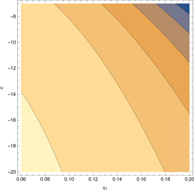
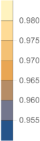
Figure 1: The spectral index of primordial curvature perturbations $n_{S}$ (left) and tensor-to-scalar ratio $r$ (right) as functions of $c$ and $\gamma_{1}$, ranging from [-20,-7] and [0.06,0.2] respectively. It can easily be inferred that the phenomenological viability of the model can be achieved for a wide range of the free parameters.

The difference between the $\xi\mathcal{G}$ and $c\xi G^{\mu\nu}\partial_{\mu}\phi\partial_{\nu}\phi$ seems to be the constants and in particular the constant $\lambda_{1}$ of the Gauss-Bonnet coupling and $c$. Our analysis showed that the parameter $\lambda_{1}$ must be orders of magnitude lesser than unity in order to achieve a phenomenologically acceptable inflationary era. However, this can be attributed to the value of $c$ which is trivial in this case. In addition, the parameters $\lambda_{1}$ and $V_{1}$ seem to affect drastically the scalar spectral index. This was also the case for $\gamma_{1}$ being $0.15$ since it was the only value capable of doing so when $\lambda_{1}$ and $V_{1}$ were fixed in these values, along with $c$, so as not to violate the approximations made. Specifically, $c$ must be negative otherwise the scalar field obtains a complex value during the first horizon crossing. Finally, the exponent of the scalar potential is $0.5642$, which as stated before is not an integer. Perhaps there exists a different designation for the free parameters of the model at hand, which is capable of not only producing an integer exponent but also produced compatible results while simultaneously the approximated equations of motion are valid. This case was not further studied.

An important comment that should be addressed here is the numerical value of the tensor spectral index $n_{T}$. Since the model was constrained so as to neglect string corrective terms, however their impact is important since they participate in both $\dot{\phi}$ and $V(\phi)$, it stands to reason that slow-roll index $\epsilon_{6}$, which is comprised of such corrections, is inferior to the first slow-roll index. This can easily be ascertained from the previous numerical values of all slow-roll indices presented above. As a result, the tensor spectral index can be reduced to its usual form

$$\centering n_{T}=-2\epsilon_{1}\,,\@add@centering$$ (35)

and recalling the approximate form of $\epsilon_{1}$ in (17) it becomes apparent that the tensor spectral index is blue shifted, meaning always negative. The only reason to obtain a red shifted index is to let $\epsilon_{6}$, become dominant and of course negative. The latter is not a possibility that can be ruled out however the first is out of the question in this formalism, given that string corrective terms where assumed to be inferior to $\dot{\phi}$ and $V(\phi)$, even though both quantities are comprised of them. Even absent, string corrections have a strong impact on the overall phenomenology indirectly.

Finally, we address the validity of the approximations made in the previous section. Concerning the slow-roll indices, it was mentioned some paragraphs above, that these respect the slow-roll conditions. Also using for example the values ($\lambda_{1}$, $V_{1}$, $N$, $\gamma_{1}$, $c$)=($10^{-8}$, $10^{3}$, 60, 0.15, -7), we have $\dot{H}\sim\mathcal{O}(10^{-1})$ whereas $H^{2}\sim\mathcal{O}(10^{2})$, so the condition $\dot{H}\ll H^{2}$ holds true. In addition, $\frac{1}{2}\dot{\phi}^{2}\sim\mathcal{O}(10^{-1})$ and similarly $V\sim\mathcal{O}(10^{2})$, so the assumption $\frac{1}{2}\dot{\phi}^{2}\ll V$ holds true. Finally, $\ddot{\phi}\sim\mathcal{O}(10^{-1})$ compared to $H\dot{\phi}\sim\mathcal{O}(10)$, so the condition $\ddot{\phi}\ll H\dot{\phi}$ holds true. Now let us see whether the rest of the assumptions made in the previous sections indeed hold true. In particular, for the first equation of motion Eq. (8), we have $24\dot{\xi}H^{3}\sim\mathcal{O}(10^{-5})$ and $9c\xi\dot{\phi}^{2}H^{2}\sim\mathcal{O}(10^{-4})$ compared to $V\sim\mathcal{O}(100)$, so the first condition in Eq. (12), namely $24\dot{\xi}H^{3}\ll V$ holds true. Also, we have $16\dot{\xi}H\dot{H}\sim\mathcal{O}(10^{-8})$, $8(\ddot{\xi}-H\dot{\xi})\sim\mathcal{O}(10^{-5})$ and $c\left(2\xi\dot{\phi}^{2}\dot{H}-6\xi\dot{\phi}^{2}H^{2}+4H\xi\dot{\phi}\ddot{\phi}+2H\dot{\xi}\dot{\phi}^{2}\right)\sim\mathcal{O}(10^{-5})$ while $\dot{\phi}^{2}\sim\mathcal{O}(10^{-1})$ hence Eq. (14) is indeed valid. Lastly, with regard to (10), we have $\xi^{\prime}\mathcal{G}\sim\mathcal{O}(10^{-3})$, $3c\left(H^{2}(\dot{\xi}\dot{H}+2\xi\ddot{\phi})+2H(2\dot{H}+3H^{2})\xi\dot{\phi}\right)\sim\mathcal{O}(10^{-3})$ while $V^{\prime}\sim\mathcal{O}(10)$. As a result, all the approximations made are valid.

Let us now return to the case of the numerical value of $c\xi$. As mentioned before, such combination is forced to take small values otherwise the model becomes unstable. Indeed, by assuming that $\lambda_{1}$ and $c$ are of order $\mathcal{O}(10^{3})$, compatibility with recent observations vanishes since now the scalar spectral index obtains an insane value of $n_{S}=3.14739$ and also $c_{A}=34$ at the end of the inflationary era, which means that causality is violated. Such a problem however is not present when the previous parameters take small values. This result is at variance with the the Gauss-Bonnet case of $\xi(\phi)\mathcal{G}$ since now $\lambda_{1}$ alters the results significantly.

As a last comment, it is worth mentioning that the choice for a cosine as a Gauss-Bonnet coupling function is also capable of producing a viable phenomenology. In particular, assuming that $\xi(\phi)=\lambda_{1}\cos(\gamma_{1}\kappa\phi)$ then by altering only $\gamma_{1}$ and $c$ to $c=-3$ and $\gamma_{1}=0.1$ manages to produce viable observed indices as $n_{S}=0.96239$, $r=0.0355884$ and $n_{T}=-0.00445847$ while simultaneously the sound wave velocity is once again equal to unity. In Fig. 2 we present the dependence of the observational indices on the same free parameters, namely $c$ and $\gamma_{1}$. Moreover, all the approximations made in the previous section, are satisfied once again. It becomes apparent that the same phenomenology is gained in the case of a cosine as well. Thus, one could argue that the general Gauss-Bonnet scalar coupling function reads $\xi(\phi)=\lambda_{1}\sin(\gamma_{1}\kappa\phi+\theta)$ where $\theta$ is an arbitrary phase, or in other words a connection between the sine and cosine description. This however does not mean that each and every trigonometric function is capable of producing a viable description. Indeed, the case of a tangent Gauss-Bonnet coupling or in general a hyperbolic trigonometric case results in complex values for the scalar field. The most promising choice would be the hyperbolic sine which produced a real scalar field, however the model, dependent on $c$ and $\gamma_{1}$, cannot produce compatible values for both the scalar spectral index of primordial curvature perturbations and the tensor-to-scalar ratio. In general, the same argument could be used for the exponential choice or an exponential like choice for the Gauss-Bonnet coupling. The choice of $\xi(\phi)=\lambda_{1}(1-e^{\gamma_{1}\kappa\phi})$ is described only by a complex scalar field and furthermore, the choice of a pure exponential, meaning $\xi(\phi)=\lambda_{1}e^{\gamma_{1}\kappa\phi}$ results in eternal or no inflation since slow-roll index $\epsilon_{1}$ turns out to be $\phi$-independent. In fact, $\epsilon_{1}=\frac{1}{2}\left(\frac{4\kappa^{2}\gamma_{1}}{4\gamma_{1}^{2}\kappa^{2}-c}\right)^{2}$ which according to the choice of $\gamma_{1}$ and $c$ leads to either eternal inflation for $\epsilon_{1}<1$ or no inflation for $\epsilon_{1}>1$. It seems that this description is suitable for trigonometric functions.

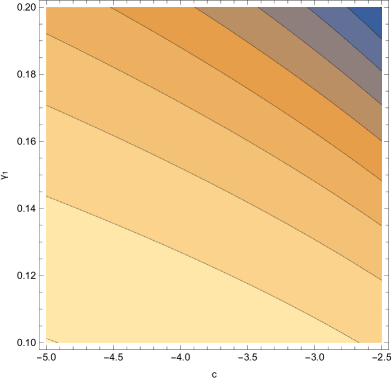
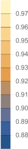
Figure 2: Scalar spectral index $n_{S}$ (left) and tensor-to-scalar ratio $r$ (right) depending on $c$ and $\gamma_{1}$, ranging from [-5,-2.5] and [0.1,0.2] respectively for the case of cosine Gauss-Bonnet coupling.

In principle there are many other models that may lead to a viable phenomenology, however we refrain from discussing other examples for brevity. The procedure is more or less the same, and nothing new is added to our argument. In the next section, we shall discuss another interesting case, the case that the scalar field evolves dynamically in a constant-roll way.

IV Inflationary Phenomenology of the GW170817-compatible Non-minimal Kinetic Coupling Corrected Einstein-Gauss-Bonnet Gravity: Constant-Roll Evolution

In this procedure, we shall study a different scenario compared to the slow-roll assumption for the scalar field. Particularly, we shall assume that the scalar field evolves dynamically in a constant-roll way Inoue:2001zt ; Tsamis:2003px ; Kinney:2005vj ; Tzirakis:2007bf ; Namjoo:2012aa ; Martin:2012pe ; Motohashi:2014ppa ; Cai:2016ngx ; Motohashi:2017aob ; Hirano:2016gmv ; Anguelova:2015dgt ; Cook:2015hma ; Kumar:2015mfa ; Odintsov:2017yud ; Odintsov:2017qpp ; Lin:2015fqa ; Gao:2017uja ; Nojiri:2017qvx ; Oikonomou:2017bjx ; Odintsov:2017hbk ; Oikonomou:2017xik ; Cicciarella:2017nls ; Awad:2017ign ; Anguelova:2017djf ; Ito:2017bnn ; Karam:2017rpw ; Yi:2017mxs ; Mohammadi:2018oku ; Gao:2018tdb ; Mohammadi:2018wfk ; Morse:2018kda ; Cruces:2018cvq ; GalvezGhersi:2018haa ; Boisseau:2018rgy ; Gao:2019sbz ; Lin:2019fcz ; Odintsov:2019ahz , and as we shall see most of the equations we used previously, shall remain the same, hence for simplicity we shall present only the equations that differ from the previous case. Essentially, the constant-roll assumption states that,

$$\ddot{\phi}=\beta H\dot{\phi}\,,$$ (36)

where $\beta$ denotes the constant-roll parameter. As a result, the overall phenomenology experiences certain changes. Firstly, the equation for the scalar field shall be rewritten. Recalling Eq. (6), in view of the constant-roll condition (36) we have,

$$\centering\dot{\phi}=\frac{4H(1-\beta)\xi^{\prime}}{4\xi^{\prime\prime}+c\xi}\,.\@add@centering$$ (37)

Here, it is worth making some comments. Firstly, this formula is exact as no approximations were made. Secondly, for $\beta\ll 1$, one obtains the same equation as in Eq. (7). Finally, as expected, for $c\to 0$, we obtain the same formula as in the case of Einstein-Gauss-Bonnet theory, either for the slow-roll or constant-roll assumption respectively. Concerning the equations of motion, they remain exactly the same, from (8)-(10). Furthermore, we shall assume the exact same approximations, meaning the slow-roll conditions and also the ones made in Eqs. (11) and (12). Thus, the simplified equations of motion read,

$$\centering H^{2}=\frac{\kappa^{2}V}{3}\,,\@add@centering$$ (38)

$$\centering\dot{H}=-\frac{\kappa^{2}H^{2}}{2}\left(\frac{4(1-\beta)\xi^{\prime}}{4\xi^{\prime\prime}+c\xi}\right)^{2}\,,\@add@centering$$ (39)

$$\centering V^{\prime}+3(1-\beta)(1+\frac{\beta}{3})H^{2}\frac{4\xi^{\prime}}{4\xi^{\prime\prime}+c\xi}=0\,.\@add@centering$$ (40)

The slow-roll indices do not experience any dramatic changes, except of course for the slow-roll index $\epsilon_{2}$. In fact, the same forms as before are still applicable with the only difference being a factor of $1-\beta$. The same applies to the auxiliary parameters $Q_{i}$ however we shall only showcase the slow-roll indices since are more important. In fact, concerning the slow-roll indices, the only significant difference is found as expected in the slow-roll index $\epsilon_{2}$, which in the case at hand is $\epsilon_{2}=\beta$. The slow-roll indices under the constant-roll assumption are shown below,

$$\centering\epsilon_{1}=\frac{1}{2}\left(\frac{4(1-\beta)\kappa\xi^{\prime}}{4\xi^{\prime\prime}+c\xi}\right)^{2}\,,\@add@centering$$ (41)

$$\centering\epsilon_{2}=\beta\,,\@add@centering$$ (42)

$$\centering\epsilon_{4}=\frac{2(1-\beta)\xi^{\prime}}{4\xi^{\prime\prime}+c\xi}\frac{E^{\prime}}{E}\,,\@add@centering$$ (43)

$$\centering\epsilon_{5}=\frac{-16(1-\beta)\frac{\xi^{\prime 2}H^{2}}{4\xi^{\prime\prime}+c\xi}+4c\xi H^{2}\left(\frac{4(1-\beta)\xi^{\prime}}{4\xi^{\prime\prime}+c\xi}\right)^{2}}{\frac{1}{\kappa^{2}}-32(1-\beta)\frac{\xi^{\prime 2}H^{2}}{4\xi^{\prime\prime}+c\xi}+32c\xi H^{2}\left(\frac{(1-\beta)\xi^{\prime}}{4\xi^{\prime\prime}+c\xi}\right)^{2}}\,,\@add@centering$$ (44)

$$\centering\epsilon_{6}=-\frac{4H^{2}\frac{4\xi^{\prime 2}(1-\beta)}{4\xi^{\prime\prime}+c\xi}(\frac{4\xi^{\prime\prime}(1-\beta)}{4\xi^{\prime\prime}+c\xi}+\beta-\epsilon_{1})+cH^{2}\left(\frac{4\xi^{\prime}(1-\beta)}{4\xi^{\prime\prime}+c\xi}\right)^{2}\left(\frac{2\xi^{\prime 2}(1-\beta)}{4\xi^{\prime\prime}+c\xi}+\xi\beta\right)}{\frac{1}{\kappa^{2}}-32\frac{\xi^{\prime 2}(1-\beta)}{4\xi^{\prime\prime}+c\xi}H^{2}+c\xi H^{2}\left(\frac{4\xi^{\prime}(1-\beta)}{4\xi^{\prime\prime}+c\xi}\right)^{2}}\,.\@add@centering$$ (45)

In this case as well, it is clear that the first two slow-roll indices are simple while the rest are perplexed. Also, only a factor of $1-\beta$ is now emergent, in contrast to the slow-roll case, as mentioned before. Lastly, the $e$-foldings number is also slightly changed in the constant-roll case, as is shown below,

$$\centering N=\frac{1}{1-\beta}\int_{\phi_{i}}^{\phi_{f}}{\frac{4\xi^{\prime\prime}+c\xi}{4\xi^{\prime}}d\phi}\,.\@add@centering$$ (46)

It can easily be inferred that the overall phenomenology is similar to the one acquired previously. In particular, for $\beta\ll 1$, the results are quite similar. In the following we shall study a specific model and examine whether the constant-roll assumption in general can produce compatible results. We shall present an interesting example with the Gauss-Bonnet scalar coupling being chosen to be a linear function of the scalar field.

IV.1 The Choice Of A Linear Gauss-Bonnet Coupling

Let us assume a simple form for the Gauss-Bonnet scalar coupling function, and particularly, let $\xi(\phi)$ be equal to,

$$\centering\xi(\phi)=\lambda_{2}\kappa\phi\,,\@add@centering$$ (47)

so $\xi(\phi)$ is a linear function of the scalar field. In this case, the second derivative with respect to the scalar field is zero, meaning $\xi^{\prime\prime}=0$. As we shall show shortly, the condition $\xi^{\prime\prime}$ being equal to zero does not affect dramatically the phenomenology, on the contrary it makes our study easier, since $\dot{\phi}$ is simplified. The corresponding scalar potential also has a power-law form, and it can easily be found for the linear scalar coupling, and it reads,

$$\centering V(\phi)=V_{2}(\kappa\phi)^{-4\frac{(1-\beta)\kappa^{2}}{c}}\,.\@add@centering$$ (48)

It is clear that the exponent is once again general and is not necessarily integer. Let us now proceed with the slow-roll indices, Due to the linear choice of the scalar coupling function, we have,

$$\centering\epsilon_{1}=2\left(\frac{2(1-\beta)\kappa}{c\phi}\right)^{2}\,.\@add@centering$$ (49)

Due to the simple form of the slow-roll index $\epsilon_{1}$, the initial and final value of the scalar field are easily obtained and in this case are written as,

$$\centering\phi_{i}=\pm\sqrt{\frac{c\phi_{f}^{2}+8N(1-\beta)^{2}}{-c}}\,,\@add@centering$$ (50)

$$\centering\phi_{f}=\pm\frac{2\kappa(1-\beta)\sqrt{2}}{c}\,.\@add@centering$$ (51)

The resulting theory can be compatible with the observational data for a wide range of values of the free parameters. For example by choosing ($\lambda_{2}$, $V_{2}$, $N$, $c$, $\beta$)=($10^{-8}$, 10, 60, -5, 0.009) in reduced Planck units ($\kappa^{2}=1$), then the observational indices read $n_{S}=0.968604$, $n_{T}=-0.0066667$ and $r=0.0531572$ which are obviously compatible with the data coming from the Planck 2018 collaboration. Moreover, the scalar field decreases with time as $\phi_{i}=9.72595$ whereas $\phi_{f}=0.560594$ in Planck units, the sound wave velocity is equal to unity as expected and in addition, the slow-roll conditions seem to be valid since the numerical values of the slow-roll indices are of order $\mathcal{O}(10^{-3})$ and lesser. In particular, $\epsilon_{1}=0.0033223$, $\epsilon_{4}=1.2\cdot 10^{-6}$, $\epsilon_{5}=-6.4\cdot 10^{-8}$ and $\epsilon_{6}=5\cdot 10^{-11}$.

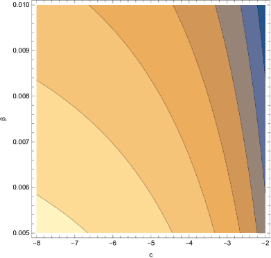
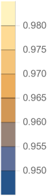
Figure 3: The scalar spectral index $n_{S}$ (left) and tensor-to-scalar ratio $r$ (right) with respect to constant-roll parameter $\beta$ and the parameter $c$. Their values range from [0.005, 0.01] and [-8,-2] respectively. It becomes apparent that spectral index $n_{S}$ depends on both the free parameters, whereas $r$ is only affected by $c$. In particular, the observational indices are very sensitive since in such small area of designation for the free parameters, the possible values for $n_{s}$ and $r$ have a wide range.

In this case, the scalar potential, which follows a power-law form as well, has an exponent which is approximately equal to $0.793$, hence once again it is not integer as expected. Perhaps there exists a complete different choice for the free parameters which produce a more familiar exponent. In Fig. 3 we present the dependence of the observational indices on the constant-roll parameter $\beta$ and the parameter $c$. In general, these are not the only parameters which affect the results. Indeed, $\lambda_{2}$ also affects the overall phenomenology as $\lambda_{2}=0.0001$ for instance produces incompatible results, namely $n_{S}=0.944381$ and $r=0.0751259$. The coefficient of the scalar potential also affects the results. Here, increasing $V_{2}$ affects mildly the scalar spectral index of the primordial curvature perturbations. On the other hand, the tensor-to-scalar ratio varies since for $V_{2}=10^{3}$, we have $r=0.0533064$ but for $V_{2}=10^{5}$, while $n_{S}$ is altered little, the tensor-to-scalar ratio is increased by an order, in particular $r=0.115128$, hence it is necessary to choose this value wisely. Referring to Fig. 3 and in particular parameter $\beta$, it becomes apparent that there exist multiple values and especially of order $\mathcal{O}(10^{-2})$ and greater which are capable of producing compatible with the observations results however in our initial example we chose to work with a value of $\mathcal{O}(10^{-3})$ for the constant-roll parameter so as to obtain a slow-roll index $\epsilon_{2}$ of equal order as the first at least. Decreasing the order is obviously viable however it gets closer to the slow-roll case hence the selection of $\beta=0.009$. Now the question is, is there any dividing line between slow-roll and constant-roll regimes? The constant-roll condition in general generates non-Gaussianities, so in principle if a constant-roll regime actually occurred, this could have observable effects, that may be observed in the future. To our opinion, a constant-roll phase occurs when $\beta$ is not a small parameter ($\beta\ll 1$), so possibly when $\beta\mathcal{(}O)(10^{-3})$ or larger a constant-roll regime is realized, this is why we chose $\beta$ taking the value $\beta=0.009$, as we discussed previously. For smaller values of $\beta$, the slow-roll regime would be approached.

Since an analysis referring to the sound wave velocity was made in the slow-roll case, it is only fair to examine the impact of the combination $c\xi$ in the constant-roll case as well. As it was shown before, this particular choice of parameters results in $c_{A}=1$. Suppose now that $\lambda_{2}\sim\mathcal{O}(10^{-3})$ and $c\sim\mathcal{O}(10^{2})$. As a result, the sound wave velocity during the ending stage of the inflationary era obtains a numerical value of $c_{A}=1.0996+0.0044i$, which is complex, therefore ghost instabilities are unavoidable. When $\lambda_{2}$ is decreased however, no instabilities are present in our description. Moreover, such an increase in parameters leads in a scalar spectral index of $n_{S}=-4.53$ which is once again an insane value. This proves once and for all that the choice of $c$ and $\lambda_{2}$ cannot be left unchecked. In principle, there could exist a pair of values for the free parameters such that $c$ and $\lambda_{2}$ are close to unity and compatibility is achieved, however to our knowledge, no such pair was found. And for consistency, even if such pair was to be found, there is a great chance that the model is infested with ghost instabilities or superluminal velocities. In conclusion, the safest way to obtain a viable phenomenology is to control the values of $c$ and $\lambda_{2}$ and constraining them to be small many orders lesser than unity.

Finally, let us discuss here and validate whether the approximations assumed in the section II hold true. Firstly, by choosing ($\lambda_{2}$, $V_{2}$, $N$, $c$, $\beta$)=($10^{-8}$, 10, 60, -5, 0.009), we have $\dot{H}\sim\mathcal{O}(10^{-2})$ compared to $H^{2}\sim\mathcal{O}(10)$, so the condition $\dot{H}\ll H^{2}$ holds true. Similarly, $\frac{1}{2}\dot{\phi}^{2}\sim\mathcal{O}(10^{-2})$ while $V\sim\mathcal{O}(10)$, so the assumption $\frac{1}{2}\dot{\phi}^{2}\ll V$ also holds true. In addition, we have $24\dot{\xi}H^{3}\sim\mathcal{O}(10^{-5})$ and $9c\xi\dot{\phi}^{2}H^{2}\sim\mathcal{O}(10^{-5})$ which are both inferior to $V\sim\mathcal{O}(10)$, so the conditions in Eq. (12), hold true. Also, $16\dot{\xi}H\dot{H}\sim\mathcal{O}(10^{-8})$, $8(\ddot{\xi}-H\dot{\xi})\sim\mathcal{O}(10^{-7})$ and $c\left(2\xi\dot{\phi}^{2}\dot{H}-6\xi\dot{\phi}^{2}H^{2}+4H\xi\dot{\phi}\ddot{\phi}+2H\dot{\xi}\dot{\phi}^{2}\right)\sim\mathcal{O}(10^{-5})$ while $\dot{\phi}^{2}\sim\mathcal{O}(10^{-1})$. Lastly, we note that $\xi^{\prime}\mathcal{G}\sim\mathcal{O}(10^{-4})$, $3c\left(H^{2}(\dot{\xi}\dot{H}+2\xi\ddot{\phi})+2H(2\dot{H}+3H^{2})\xi\dot{\phi}\right)\sim\mathcal{O}(10^{-3})$ while $V^{\prime}\sim\mathcal{O}(1)$. Thus, all the approximations made are indeed valid.

As a result, the kinetic coupling-corrected Einstein-Gauss-Bonnet gravity with a linear coupling function, can lead to a viable phenomenology assuming that graviton is massless. This is in contrast to the simple GW170817-compatible Einstein-Gauss-Bonnet gravity, which as we show in Ref. EPL , a linear coupling leads to the constant-roll condition inevitably, and the resulting theory is phenomenologically questionable, with the regard to the inflationary phenomenology. Actually, as we show in EPL , the resulting scalar spectral index is always quite close to the value $n_{S}\sim-1$.

V Conclusions

In this work we studied non-minimal kinetic coupling corrected Einstein-Gauss-Bonnet theories in view of the GW17017 event, which restricted the gravitational wave speed to be equal to that of light’s. The constraint $c_{T}^{2}=1$ as we showed, constrained the functional form of the scalar coupling and of the scalar potential, and by using the slow-roll assumption, we showed how a viable phenomenology can be obtained by the present theoretical framework. We derived analytic formulas for the slow-roll indices and for the observational characterizing the inflationary era, and by using several illustrative examples, we demonstrated how the compatibility of the inflationary phenomenology corresponding to the present theory can be achieved. In principle several choices of the scalar coupling function can also yield viable results, but we refrained from presenting more models than a small class of models, for brevity.

Our motivation of imposing the constraint $c_{T}^{2}=1$ in the primordial gravitational waves, is mainly the fact that there is no particle physics process related to the inflationary and post-inflationary era that alters the graviton mass. The graviton has a specific mass which can be determined by the string theory governing the physics of the pre-inflationary epoch, so if the graviton mass is specific during the inflationary era, there is no fundamental reason that may allow it to change, at least to our knowledge. As we showed, the constraint $c_{T}^{2}=1$ actually leads to a phenomenologically viable non-minimal kinetic coupling corrected Einstein-Gauss-Bonnet inflationary theory. Also, it is worth mentioning that the constraint $c_{T}^{2}=1$ for the non-minimal kinetic coupling corrected Einstein-Gauss-Bonnet also covers theories with string correction terms of the form, results to the same differential equation $\sim\xi(\phi)\Box\phi g^{\mu\nu}\partial_{\mu}\phi\partial_{\nu}\phi$ and $\sim\xi(\phi)\left(g^{\mu\nu}\partial_{\mu}\phi\partial_{\nu}\phi\right)^{2}$, in which case the full effective Lagrangian is of the form,

$$\centering\mathcal{S}=\int{d^{4}x\sqrt{-g}\left(\frac{R}{2\kappa^{2}}-\frac{1}{2}g^{\mu\nu}\partial_{\mu}\phi\partial_{\nu}\phi-V(\phi)-\xi(\phi)\mathcal{G}-c\xi(\phi)G^{\mu\nu}\partial_{\mu}\phi\partial_{\nu}\phi-c_{1}\Box\phi g^{\mu\nu}\partial_{\mu}\phi\partial_{\nu}\phi-c_{2}\left(g^{\mu\nu}\partial_{\mu}\phi\partial_{\nu}\phi\right)^{2}\right)}\,.\@add@centering$$ (52)

Theories of the form (52) belong to a wider class of Horndeski theories, so in this paper we demonstrated how these theories may be revived formally, in view of the GW170817 event. We did not study in detail however theories of the form (52) since with this paper we just wanted to demonstrate how the simplest class of these theories can be revived. In a future work we might address in detail the analysis of the full theory.

Finally, we discussed also the constant-roll scenario in the context of the present theory. It is interesting to note that the constant-roll condition is related to non-Gaussianities Odintsov:2019ahz ; Martin:2012pe , so in a future work it would be interesting to address this issue in detail in the context of the non-minimal kinetic coupling corrected Einstein-Gauss-Bonnet theories.

Finally, it is interesting to comment on the effects of the constant-roll phase on the reheating era. This issue is non-trivial to simply answer in a straightforward manner, and needs to be addressed in detail in a future work, since for $F(R)$ gravity, a constant-roll phase alters the reheating temperature, as was shown in Ref. Oikonomou:2017bjx .

References

- (1) J. c. Hwang and H. Noh, Phys. Rev. D 71 (2005) 063536 doi:10.1103/PhysRevD.71.063536 [gr-qc/0412126].
- (2) S. Nojiri, S. D. Odintsov and M. Sami, Phys. Rev. D 74 (2006) 046004 doi:10.1103/PhysRevD.74.046004 [hep-th/0605039].
- (3) G. Cognola, E. Elizalde, S. Nojiri, S. Odintsov and S. Zerbini, Phys. Rev. D 75 (2007) 086002 doi:10.1103/PhysRevD.75.086002 [hep-th/0611198].
- (4) S. Nojiri, S. D. Odintsov and M. Sasaki, Phys. Rev. D 71 (2005) 123509 doi:10.1103/PhysRevD.71.123509 [hep-th/0504052].
- (5) S. Nojiri and S. D. Odintsov, Phys. Lett. B 631 (2005) 1 doi:10.1016/j.physletb.2005.10.010 [hep-th/0508049].
- (6) M. Satoh, S. Kanno and J. Soda, Phys. Rev. D 77 (2008) 023526 doi:10.1103/PhysRevD.77.023526 [arXiv:0706.3585 [astro-ph]].
- (7) K. Bamba, A. N. Makarenko, A. N. Myagky and S. D. Odintsov, JCAP 1504 (2015) 001 doi:10.1088/1475-7516/2015/04/001 [arXiv:1411.3852 [hep-th]].
- (8) Z. Yi, Y. Gong and M. Sabir, Phys. Rev. D 98 (2018) no.8, 083521 doi:10.1103/PhysRevD.98.083521 [arXiv:1804.09116 [gr-qc]].
- (9) Z. K. Guo and D. J. Schwarz, Phys. Rev. D 80 (2009) 063523 doi:10.1103/PhysRevD.80.063523 [arXiv:0907.0427 [hep-th]].
- (10) Z. K. Guo and D. J. Schwarz, Phys. Rev. D 81 (2010) 123520 doi:10.1103/PhysRevD.81.123520 [arXiv:1001.1897 [hep-th]].
- (11) P. X. Jiang, J. W. Hu and Z. K. Guo, Phys. Rev. D 88 (2013) 123508 doi:10.1103/PhysRevD.88.123508 [arXiv:1310.5579 [hep-th]].
- (12) P. Kanti, R. Gannouji and N. Dadhich, Phys. Rev. D 92 (2015) no.4, 041302 doi:10.1103/PhysRevD.92.041302 [arXiv:1503.01579 [hep-th]].
- (13) C. van de Bruck, K. Dimopoulos, C. Longden and C. Owen, arXiv:1707.06839 [astro-ph.CO].
- (14) P. Kanti, J. Rizos and K. Tamvakis, Phys. Rev. D 59 (1999) 083512 doi:10.1103/PhysRevD.59.083512 [gr-qc/9806085].
- (15) S. Kawai and J. Soda, Phys. Lett. B 460 (1999) 41 doi:10.1016/S0370-2693(99)00736-4 [gr-qc/9903017].
- (16) K. Nozari and N. Rashidi, Phys. Rev. D 95 (2017) no.12, 123518 doi:10.1103/PhysRevD.95.123518 [arXiv:1705.02617 [astro-ph.CO]].
- (17) S. Chakraborty, T. Paul and S. SenGupta, Phys. Rev. D 98 (2018) no.8, 083539 doi:10.1103/PhysRevD.98.083539 [arXiv:1804.03004 [gr-qc]].
- (18) S. D. Odintsov and V. K. Oikonomou, Phys. Rev. D 98 (2018) no.4, 044039 doi:10.1103/PhysRevD.98.044039 [arXiv:1808.05045 [gr-qc]].
- (19) S. Kawai, M. a. Sakagami and J. Soda, Phys. Lett. B 437, 284 (1998) doi:10.1016/S0370-2693(98)00925-3 [gr-qc/9802033].
- (20) Z. Yi and Y. Gong, Universe 5 (2019) no.9, 200 doi:10.3390/universe5090200 [arXiv:1811.01625 [gr-qc]].
- (21) C. van de Bruck, K. Dimopoulos and C. Longden, Phys. Rev. D 94 (2016) no.2, 023506 doi:10.1103/PhysRevD.94.023506 [arXiv:1605.06350 [astro-ph.CO]].
- (22) B. Kleihaus, J. Kunz and P. Kanti, arXiv:1910.02121 [gr-qc].
- (23) A. Bakopoulos, P. Kanti and N. Pappas, Phys. Rev. D 101 (2020) no.4, 044026 doi:10.1103/PhysRevD.101.044026 [arXiv:1910.14637 [hep-th]].
- (24) K. i. Maeda, N. Ohta and R. Wakebe, Eur. Phys. J. C 72 (2012) 1949 doi:10.1140/epjc/s10052-012-1949-6 [arXiv:1111.3251 [hep-th]].
- (25) A. Bakopoulos, P. Kanti and N. Pappas, arXiv:2003.02473 [hep-th].
- (26) W. Ai, [arXiv:2004.02858 [gr-qc]].
- (27) R. Easther and K. i. Maeda, Phys. Rev. D 54 (1996) 7252 doi:10.1103/PhysRevD.54.7252 [hep-th/9605173].
- (28) I. Antoniadis, J. Rizos and K. Tamvakis, Nucl. Phys. B 415 (1994) 497 doi:10.1016/0550-3213(94)90120-1 [hep-th/9305025].
- (29) I. Antoniadis, C. Bachas, J. R. Ellis and D. V. Nanopoulos, Phys. Lett. B 257 (1991), 278-284 doi:10.1016/0370-2693(91)91893-Z
- (30) S. Odintsov, V. Oikonomou and F. Fronimos, [arXiv:2003.13724 [gr-qc]].
- (31) S. Odintsov and V. Oikonomou, Phys. Lett. B 805 (2020), 135437 doi:10.1016/j.physletb.2020.135437 [arXiv:2004.00479 [gr-qc]].
- (32) S. D. Odintsov and V. K. Oikonomou, Phys. Lett. B 797 (2019) 134874 doi:10.1016/j.physletb.2019.134874 [arXiv:1908.07555 [gr-qc]].
- (33) J. M. Ezquiaga and M. Zumalacarregui, Phys. Rev. Lett. 119 (2017) no.25, 251304 doi:10.1103/PhysRevLett.119.251304 [arXiv:1710.05901 [astro-ph.CO]].
- (34) B. P. Abbott et al. “Multi-messenger Observations of a Binary Neutron Star Merger,” Astrophys. J. 848 (2017) no.2, L12 doi:10.3847/2041-8213/aa91c9 [arXiv:1710.05833 [astro-ph.HE]].
- (35) S. Nojiri, S. D. Odintsov and V. K. Oikonomou, Phys. Rept. 692 (2017) 1 doi:10.1016/j.physrep.2017.06.001 [arXiv:1705.11098 [gr-qc]].
- (36) S. Nojiri and S. D. Odintsov, Phys. Rept. 505 (2011) 59 doi:10.1016/j.physrep.2011.04.001 [arXiv:1011.0544 [gr-qc]].
- (37) S. Nojiri and S. D. Odintsov, eConf C 0602061 (2006) 06 [Int. J. Geom. Meth. Mod. Phys. 4 (2007) 115] doi:10.1142/S0219887807001928 [hep-th/0601213].
- (38) S. Capozziello and M. De Laurentis, Phys. Rept. 509 (2011) 167 doi:10.1016/j.physrep.2011.09.003 [arXiv:1108.6266 [gr-qc]].
- (39) V. Faraoni and S. Capozziello, Fundam. Theor. Phys. 170 (2010). doi:10.1007/978-94-007-0165-6
- (40) A. de la Cruz-Dombriz and D. Saez-Gomez, Entropy 14 (2012) 1717 doi:10.3390/e14091717 [arXiv:1207.2663 [gr-qc]].
- (41) G. J. Olmo, Int. J. Mod. Phys. D 20 (2011) 413 doi:10.1142/S0218271811018925 [arXiv:1101.3864 [gr-qc]].
- (42) Y. Akrami et al. [Planck Collaboration], arXiv:1807.06211 [astro-ph.CO].
- (43) G. W. Horndeski, Int.J.Theor.Phys. 10, 363 (1974).
- (44) T. Kobayashi, Rept. Prog. Phys. 82 (2019) no.8, 086901 doi:10.1088/1361-6633/ab2429 [arXiv:1901.07183 [gr-qc]].
- (45) T. Kobayashi, Phys. Rev. D 94 (2016) no.4, 043511 doi:10.1103/PhysRevD.94.043511 [arXiv:1606.05831 [hep-th]].
- (46) M. Crisostomi, M. Hull, K. Koyama and G. Tasinato, JCAP 03 (2016), 038 doi:10.1088/1475-7516/2016/03/038 [arXiv:1601.04658 [hep-th]].
- (47) E. Bellini, A. J. Cuesta, R. Jimenez and L. Verde, JCAP 02 (2016), 053 doi:10.1088/1475-7516/2016/06/E01 [arXiv:1509.07816 [astro-ph.CO]].
- (48) J. Gleyzes, D. Langlois, F. Piazza and F. Vernizzi, JCAP 02 (2015), 018 doi:10.1088/1475-7516/2015/02/018 [arXiv:1408.1952 [astro-ph.CO]].
- (49) C. Lin, S. Mukohyama, R. Namba and R. Saitou, JCAP 10 (2014), 071 doi:10.1088/1475-7516/2014/10/071 [arXiv:1408.0670 [hep-th]].
- (50) C. Deffayet and D. A. Steer, Class. Quant. Grav. 30 (2013), 214006 doi:10.1088/0264-9381/30/21/214006 [arXiv:1307.2450 [hep-th]].
- (51) D. Bettoni and S. Liberati, Phys. Rev. D 88 (2013), 084020 doi:10.1103/PhysRevD.88.084020 [arXiv:1306.6724 [gr-qc]].
- (52) K. Koyama, G. Niz and G. Tasinato, Phys. Rev. D 88 (2013), 021502 doi:10.1103/PhysRevD.88.021502 [arXiv:1305.0279 [hep-th]].
- (53) A. A. Starobinsky, S. V. Sushkov and M. S. Volkov, JCAP 06 (2016), 007 doi:10.1088/1475-7516/2016/06/007 [arXiv:1604.06085 [hep-th]].
- (54) S. Capozziello, K. F. Dialektopoulos and S. V. Sushkov, Eur. Phys. J. C 78 (2018) no.6, 447 doi:10.1140/epjc/s10052-018-5939-1 [arXiv:1803.01429 [gr-qc]].
- (55) J. Ben Achour, M. Crisostomi, K. Koyama, D. Langlois, K. Noui and G. Tasinato, JHEP 12 (2016), 100 doi:10.1007/JHEP12(2016)100 [arXiv:1608.08135 [hep-th]].
- (56) A. A. Starobinsky, S. V. Sushkov and M. S. Volkov, Phys. Rev. D 101 (2020) no.6, 064039 doi:10.1103/PhysRevD.101.064039 [arXiv:1912.12320 [hep-th]].
- (57) S. V. Sushkov, Phys. Rev. D 80 (2009), 103505 doi:10.1103/PhysRevD.80.103505 [arXiv:0910.0980 [gr-qc]].
- (58) M. Minamitsuji, Phys. Rev. D 89 (2014), 064017 doi:10.1103/PhysRevD.89.064017 [arXiv:1312.3759 [gr-qc]].
- (59) E. N. Saridakis and S. V. Sushkov, Phys. Rev. D 81 (2010), 083510 doi:10.1103/PhysRevD.81.083510 [arXiv:1002.3478 [gr-qc]].
- (60) A. Barreira, B. Li, A. Sanchez, C. M. Baugh and S. Pascoli, Phys. Rev. D 87 (2013), 103511 doi:10.1103/PhysRevD.87.103511 [arXiv:1302.6241 [astro-ph.CO]].
- (61) S. Sushkov, Phys. Rev. D 85 (2012), 123520 doi:10.1103/PhysRevD.85.123520 [arXiv:1204.6372 [gr-qc]].
- (62) A. Barreira, B. Li, C. M. Baugh and S. Pascoli, Phys. Rev. D 86 (2012), 124016 doi:10.1103/PhysRevD.86.124016 [arXiv:1208.0600 [astro-ph.CO]].
- (63) M. A. Skugoreva, S. V. Sushkov and A. V. Toporensky, Phys. Rev. D 88 (2013), 083539 doi:10.1103/PhysRevD.88.083539 [arXiv:1306.5090 [gr-qc]].
- (64) G. Gubitosi and E. V. Linder, Phys. Lett. B 703 (2011), 113-118 doi:10.1016/j.physletb.2011.07.066 [arXiv:1106.2815 [astro-ph.CO]].
- (65) J. Matsumoto and S. V. Sushkov, JCAP 11 (2015), 047 doi:10.1088/1475-7516/2015/11/047 [arXiv:1510.03264 [gr-qc]].
- (66) C. Deffayet, O. Pujolas, I. Sawicki and A. Vikman, JCAP 10 (2010), 026 doi:10.1088/1475-7516/2010/10/026 [arXiv:1008.0048 [hep-th]].
- (67) L. Granda and W. Cardona, JCAP 07 (2010), 021 doi:10.1088/1475-7516/2010/07/021 [arXiv:1005.2716 [hep-th]].
- (68) J. Matsumoto and S. V. Sushkov, JCAP 01 (2018), 040 doi:10.1088/1475-7516/2018/01/040 [arXiv:1703.04966 [gr-qc]].
- (69) C. Gao, JCAP 06 (2010), 023 doi:10.1088/1475-7516/2010/06/023 [arXiv:1002.4035 [gr-qc]].
- (70) L. Granda, JCAP 07 (2010), 006 doi:10.1088/1475-7516/2010/07/006 [arXiv:0911.3702 [hep-th]].
- (71) C. Germani and A. Kehagias, Phys. Rev. Lett. 105 (2010), 011302 doi:10.1103/PhysRevLett.105.011302 [arXiv:1003.2635 [hep-ph]].
- (72) C. Fu, P. Wu and H. Yu, Phys. Rev. D 100 (2019) no.6, 063532 doi:10.1103/PhysRevD.100.063532 [arXiv:1907.05042 [astro-ph.CO]].
- (73) A. Dima and F. Vernizzi, Phys. Rev. D 97 (2018) no.10, 101302 doi:10.1103/PhysRevD.97.101302 [arXiv:1712.04731 [gr-qc]].
- (74) C. Kreisch and E. Komatsu, JCAP 12 (2018), 030 doi:10.1088/1475-7516/2018/12/030 [arXiv:1712.02710 [astro-ph.CO]].
- (75) S. Arai and A. Nishizawa, Phys. Rev. D 97 (2018) no.10, 104038 doi:10.1103/PhysRevD.97.104038 [arXiv:1711.03776 [gr-qc]].
- (76) V. Oikonomou, EPL 130 (2020) no.1, 10006 doi:10.1209/0295-5075/130/10006 [arXiv:2004.10778 [gr-qc]].
- (77) S. Inoue and J. Yokoyama, Phys. Lett. B 524 (2002) 15 doi:10.1016/S0370-2693(01)01369-7 [hep-ph/0104083].
- (78) N. C. Tsamis and R. P. Woodard, Phys. Rev. D 69 (2004) 084005 doi:10.1103/PhysRevD.69.084005 [astro-ph/0307463].
- (79) W. H. Kinney, Phys. Rev. D 72 (2005) 023515 doi:10.1103/PhysRevD.72.023515 [gr-qc/0503017].
- (80) K. Tzirakis and W. H. Kinney, Phys. Rev. D 75 (2007) 123510 doi:10.1103/PhysRevD.75.123510 [astro-ph/0701432].
- (81) M. H. Namjoo, H. Firouzjahi and M. Sasaki, Europhys. Lett. 101 (2013) 39001 doi:10.1209/0295-5075/101/39001 [arXiv:1210.3692 [astro-ph.CO]].
- (82) J. Martin, H. Motohashi and T. Suyama, Phys. Rev. D 87 (2013) no.2, 023514 doi:10.1103/PhysRevD.87.023514 [arXiv:1211.0083 [astro-ph.CO]].
- (83) H. Motohashi, A. A. Starobinsky and J. Yokoyama, JCAP 1509 (2015) no.09, 018 doi:10.1088/1475-7516/2015/09/018 [arXiv:1411.5021 [astro-ph.CO]].
- (84) Y. F. Cai, J. O. Gong, D. G. Wang and Z. Wang, JCAP 1610 (2016) no.10, 017 doi:10.1088/1475-7516/2016/10/017 [arXiv:1607.07872 [astro-ph.CO]].
- (85) H. Motohashi and A. A. Starobinsky, arXiv:1702.05847 [astro-ph.CO].
- (86) S. Hirano, T. Kobayashi and S. Yokoyama, Phys. Rev. D 94 (2016) no.10, 103515 doi:10.1103/PhysRevD.94.103515 [arXiv:1604.00141 [astro-ph.CO]].
- (87) L. Anguelova, Nucl. Phys. B 911 (2016) 480 doi:10.1016/j.nuclphysb.2016.08.020 [arXiv:1512.08556 [hep-th]].
- (88) J. L. Cook and L. M. Krauss, JCAP 1603 (2016) no.03, 028 doi:10.1088/1475-7516/2016/03/028 [arXiv:1508.03647 [astro-ph.CO]].
- (89) K. S. Kumar, J. Marto, P. Vargas Moniz and S. Das, JCAP 1604 (2016) no.04, 005 doi:10.1088/1475-7516/2016/04/005 [arXiv:1506.05366 [gr-qc]].
- (90) S. D. Odintsov and V. K. Oikonomou, arXiv:1703.02853 [gr-qc].
- (91) S. D. Odintsov and V. K. Oikonomou, arXiv:1704.02931 [gr-qc].
- (92) J. Lin, Q. Gao and Y. Gong, Mon. Not. Roy. Astron. Soc. 459 (2016) no.4, 4029 doi:10.1093/mnras/stw915 [arXiv:1508.07145 [gr-qc]].
- (93) Q. Gao and Y. Gong, arXiv:1703.02220 [gr-qc].
- (94) S. Nojiri, S. D. Odintsov and V. K. Oikonomou, Class. Quant. Grav. 34 (2017) no.24, 245012 doi:10.1088/1361-6382/aa92a4 [arXiv:1704.05945 [gr-qc]].
- (95) V. K. Oikonomou, Mod. Phys. Lett. A 32 (2017) no.33, 1750172 doi:10.1142/S0217732317501723 [arXiv:1706.00507 [gr-qc]].
- (96) S. D. Odintsov, V. K. Oikonomou and L. Sebastiani, Nucl. Phys. B 923 (2017) 608 doi:10.1016/j.nuclphysb.2017.08.018 [arXiv:1708.08346 [gr-qc]].
- (97) V. K. Oikonomou, Int. J. Mod. Phys. D 27 (2017) no.02, 1850009 doi:10.1142/S0218271818500098 [arXiv:1709.02986 [gr-qc]].
- (98) F. Cicciarella, J. Mabillard and M. Pieroni, JCAP 1801 (2018) no.01, 024 doi:10.1088/1475-7516/2018/01/024 [arXiv:1709.03527 [astro-ph.CO]].
- (99) A. Awad, W. El Hanafy, G. G. L. Nashed, S. D. Odintsov and V. K. Oikonomou, JCAP 1807 (2018) no.07, 026 doi:10.1088/1475-7516/2018/07/026 [arXiv:1710.00682 [gr-qc]].
- (100) L. Anguelova, P. Suranyi and L. C. R. Wijewardhana, JCAP 1802 (2018) no.02, 004 doi:10.1088/1475-7516/2018/02/004 [arXiv:1710.06989 [hep-th]].
- (101) A. Ito and J. Soda, Eur. Phys. J. C 78 (2018) no.1, 55 doi:10.1140/epjc/s10052-018-5534-5 [arXiv:1710.09701 [hep-th]].
- (102) A. Karam, L. Marzola, T. Pappas, A. Racioppi and K. Tamvakis, JCAP 1805 (2018) no.05, 011 doi:10.1088/1475-7516/2018/05/011 [arXiv:1711.09861 [astro-ph.CO]].
- (103) Z. Yi and Y. Gong, JCAP 1803 (2018) no.03, 052 doi:10.1088/1475-7516/2018/03/052 [arXiv:1712.07478 [gr-qc]].
- (104) A. Mohammadi, K. Saaidi and T. Golanbari, Phys. Rev. D 97 (2018) no.8, 083006 doi:10.1103/PhysRevD.97.083006 [arXiv:1801.03487 [hep-ph]].
- (105) Q. Gao, Y. Gong and Q. Fei, JCAP 1805 (2018) no.05, 005 doi:10.1088/1475-7516/2018/05/005 [arXiv:1801.09208 [gr-qc]].
- (106) A. Mohammadi and K. Saaidi, arXiv:1803.01715 [astro-ph.CO].
- (107) M. J. P. Morse and W. H. Kinney, Phys. Rev. D 97 (2018) no.12, 123519 doi:10.1103/PhysRevD.97.123519 [arXiv:1804.01927 [astro-ph.CO]].
- (108) D. Cruces, C. Germani and T. Prokopec, JCAP 1903 (2019) no.03, 048 doi:10.1088/1475-7516/2019/03/048 [arXiv:1807.09057 [gr-qc]].
- (109) J. T. Galvez Ghersi, A. Zucca and A. V. Frolov, JCAP 1905 (2019) no.05, 030 doi:10.1088/1475-7516/2019/05/030 [arXiv:1808.01325 [astro-ph.CO]].
- (110) B. Boisseau and H. Giacomini, arXiv:1809.09169 [gr-qc].
- (111) Q. Gao, Y. Gong and Z. Yi, arXiv:1901.04646 [gr-qc].
- (112) W. C. Lin, M. J. P. Morse and W. H. Kinney, arXiv:1904.06289 [astro-ph.CO].
- (113) S. Odintsov and V. Oikonomou, Class. Quant. Grav. 37 (2020) no.2, 025003 doi:10.1088/1361-6382/ab5c9d [arXiv:1912.00475 [gr-qc]].
- (114) V. K. Oikonomou and F. P. Fronimos, [arXiv:2007.11915 [gr-qc]].
- (115) V. K. Oikonomou, Mod. Phys. Lett. A 32 (2017) no.33, 1750172 doi:10.1142/S0217732317501723 [arXiv:1706.00507 [gr-qc]].