Effective field theory for acoustic and pseudo-acoustic phonons in solids

Abstract

We present a relativistic effective field theory for the interaction between acoustic and gapped phonons in the limit of a small gap. We show that, while the former are the Goldstone modes associated with the spontaneous breaking of spacetime symmetries, the latter are pseudo-Goldstones associated with some (small) explicit breaking. We hence dub them “pseudo-acoustic” phonons. In this first investigation, we build our effective theory for the cases of one and two spatial dimensions, two atomic species, and assuming large distance isotropy. As an illustrative example, we show how the theory can be applied to compute the total lifetime of both acoustic and pseudo-acoustic phonons. This construction can find applications that range from the physics of bilayer graphene to sub-GeV dark matter detectors.

I Introduction

Many properties of solids are dictated by the dynamics of their simplest collective excitations: the phonons. These are localized vibrational modes that, when characterized by wavelengths much larger than the atomic spacing, can be described in terms of quasiparticles. In a solid with a single atom per unit cell the phonons’ dispersion relation is gapless; i.e., when its wave vector vanishes so does its frequency. In this case one talks about “acoustic” phonons. However, for more complicated (and common) solids, some phonons can be gapped, with a frequency that tends to a finite positive value at zero wave vector. When the gap is comparable to or larger than the maximum frequency of the acoustic phonons, these modes are typically called “optical” phonons.

It is well known that acoustic phonons are Goldstone bosons associated with the spontaneous breaking of spatial translations induced by a solid background Leutwyler (1997). Taking this idea as a starting point, we see that recent years have witnessed the development of relativistic effective field theories (EFTs), based on symmetry breaking and its consequences, applied to the study of collective excitations in different media (see Son (2002); Endlich et al. (2013); Nicolis et al. (2015) and references therein). An EFT description of the phonons, organized in a low-energy/long wavelength expansion, has the advantage of being universal; i.e., it does not rely on the often complicated microscopic physics, up to a finite number of effective coefficients. The latter must be obtained from experiment or determined in other ways, as, for example, density functional theory (DFT) calculations—see, e.g., Kohn and Sham (1965); Saha et al. (2008); Ulman and Narasimhan (2014); Carr et al. (2018); Burke and Wagner (2013). Such an EFT approach has already proven to be useful to a number of phenomenologically relevant problems, covering a wide range of fields, from the physics of ⁴He to cosmology (see, e.g., Golkar et al. (2014); Horn et al. (2015); Crossley et al. (2017); Nicolis and Penco (2018); Rothstein and Shrivastava (2019); Moroz et al. (2018); Alberte et al. (2019); Esposito et al. (2019); Acanfora et al. (2019); Caputo et al. (2020, 2019)).

In this paper we develop a new relativistic EFT for the description of the interactions of acoustic and gapped phonons in a solid, in the regime where the gap is small compared to the typical frequency characterizing the microscopic system. For reasons that will be clear soon, we dub these collective excitations “pseudo-acoustic” phonons. See Fig. 1 for a schematic representation of the phonon spectrum. To the best of our knowledge, no bottom-up effective description of pseudo-acoustic phonons has been presented thus far.

This construction can be applied to any number of spatial dimensions and any number of atomic species within the solid. However, as we will show, we expect a small gap for the pseudo-acoustic phonons to arise when the different species are weakly coupled to each other. Such an instance is realized, for example, in few-layer materials such as graphene Saha et al. (2008); Poncharal et al. (2008); Ghosh et al. (2010); Jiang et al. (2012); Lindsay et al. (2011); Nika and Balandin (2012); Cocemasov et al. (2013); Nika and Balandin (2017), hexagonal boron nitride Michel and Verberck (2011); D’Souza and Mukherjee (2017), or a combination of the two Gholivand and Donmezer (2017). Indeed, we expect pseudo-acoustic phonons to arise in approximately two-dimensional materials every time the layers are weakly coupled to each other. In three dimensions, this situation might be harder to envision. Nevertheless, we notice that the spectrum of both graphite and three-dimensional hexagonal boron nitride exhibits phonon branches that closely resemble pseudo-acoustic modes Kern et al. (1999); Wirtz and Rubio (2004); Reich et al. (2005); Michel and Verberck (2008); Gholivand and Donmezer (2017).

In this first study, we focus on solids that are both homogeneous and isotropic at large distances. While the first property is always true, the second one is a simplifying assumption. The extension of our EFT to the case of solids which preserve only discrete rotations at large distances is straightforward, but tedious.

In constructing the EFT for acoustic and pseudo-acoustic phonons we impose relativistic Lorentz invariance. Although this might not be common in solid-state physics, there are reasons why this approach is worth exploring. First, it is technically easier to impose the Lorentz symmetry than the nonrelativistic Galilei one, by simply contracting covariant indices. Moreover, given that the Lorentz group is more fundamental, one is always free to require invariance under it, and hence allow the EFT to include relativistic effects on the phonon dynamics. The nonrelativistic limit can always be taken afterward, by reintroducing the speed of light with simple dimensional analysis and formally sending it to infinity (see, e.g., Esposito et al. (2019)). That being said, if the system of interest is nonrelativistic, there is no conceptual obstruction in imposing invariance under Galilei boosts right away. Finally, the formulation of an EFT in relativistic language also provides a useful connection to high energy physics, for example, enabling observables to be computed using techniques more familiar to this community.

One promising application of this is in the use of EFTs for describing the interactions of sub-GeV dark matter with a detector. A number of recent proposals utilize dark matter scattering off phonons in various materials as a detection mechanism; see, e.g., Hochberg et al. (2016); Guo and McKinsey (2013); Schutz and Zurek (2016); Knapen et al. (2017); Acanfora et al. (2019); Caputo et al. (2019, 2020); Baym et al. (2020); Knapen et al. (2018); Campbell-Deem et al. (2020); Griffin et al. (2018, 2020); Trickle et al. (2020); Arvanitaki et al. (2018); Bunting et al. (2017); Chen et al. (2020); Cox et al. (2019). For low-mass dark matter with a large de Broglie wavelength, an effective description of the coupling between dark matter and collective modes in the detector is necessary, since the microscopic features are not resolved. The EFT approach we follow can be extended to capture the most general dark matter–detector interaction, which is necessary for studying generic rates and differential rates of dark matter scattering. Furthermore, curious cancellation mechanisms have been observed in low-mass dark matter scattering rates in liquid helium that are transparent in the EFT Knapen et al. (2017); Caputo et al. (2019). Similar cancellations have been observed in traditional calculations of dark matter scattering off gapped and acoustic phonons in crystals Cox et al. (2019); Campbell-Deem et al. (2020). The EFT we introduce could provide new insight into these mechanisms. It could also be utilized to calculate rates of dark matter scattering off previously unconsidered pseudo-acoustic phonons, which lie in an interesting region between acoustic and optical phonons (the former having a larger scattering rate, the latter being gapped and thus having more favorable kinematics to match those of dark matter Knapen et al. (2018)); this could in turn provide the impetus to consider materials that have pseudo-acoustic phonons as dark matter detectors.

The EFT of pseudo-acoustic phonons could also find application in “solid” theories of inflation; see Endlich et al. (2013).

II EFT for Acoustic and Pseudo-Acoustic Phonons

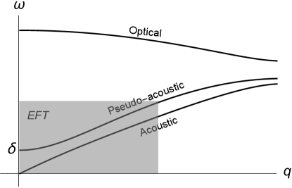
Figure 1: Schematic representation of the energy of different phonon modes as a function of momentum. The shaded region indicates where our EFT is valid.

We now describe the EFT for pseudo-acoustic and acoustic phonons, focusing on the simple cases of one and two spatial dimensions, as well as two atomic species.

1D case

Consider for a moment a monoatomic solid Endlich et al. (2013); Nicolis et al. (2015); Esposito et al. (2019). Its volume elements can be labeled with a single scalar field, $\phi(x)$—the comoving coordinate—which at equilibrium can be taken to be proportional to the physical spatial coordinate, $\langle\phi(x)\rangle=\alpha x$, where $\alpha$ is a constant determining the degree of compression/dilation of the solid Landau and Lifshitz (1986). From an EFT viewpoint this vacuum expectation value breaks boosts and spatial translations. Since all solids are homogeneous at large distances, one also postulates an internal $U(1)$ shift symmetry, $\phi\to\phi+c$, which is broken together with part of the Poincaré group down to time translations and a diagonal $U(1)$, i.e., $ISO(1,1)\times U(1)\to\mathbb{R}_{t}\times U(1)$. It is this last unbroken $U(1)$ that one uses to define large distance homogeneity.

The fluctuation of the comoving coordinate around its equilibrium configuration, $\phi(x)=\alpha x+\pi(x)$, is the Goldstone boson associated with the broken symmetries, corresponding to the phonon of the solid. As the breaking is spontaneous, the phonon dynamics must be described via a Lagrangian that is invariant under the full initial group. In the long wavelength limit (i.e., at lowest order in a derivative expansion), the only quantity that is invariant under both Poincaré transformations and the internal shift symmetry is $X=\partial_{\mu}\phi\partial^{\mu}\phi$, and the most general Lagrangian is $F(X)$, with $F$ an a priori generic function. Upon inspecting the stress-energy tensor of the theory, one finds that $F$ is simply minus the energy density Endlich et al. (2013). For a strongly coupled system its analytical expression is hard (or even impossible) to compute, and one must obtain it from experimental or numerical data.

Expanding the action in small fluctuations one obtains all possible interactions for the acoustic phonon which, being a Goldstone boson, is gapless—for details see, e.g., Endlich et al. (2013).

Let us now consider a second atomic species in our solid. One can introduce two comoving coordinates, $\phi_{A,B}(x)$, one for each species, featuring two independent shift symmetries. At equilibrium both of them are proportional to space, $\langle\phi_{A}(x)\rangle=\alpha x$ and $\langle\phi_{B}(x)\rangle=\beta x$, and the symmetry breaking pattern is then $ISO(1,1)\times U_{A}(1)\times U_{B}(1)\to\mathbb{R}_{t}\times U(1)$. Despite the number of broken generators, the system features only two Goldstones, as dictated by the inverse Higgs constraints Ivanov and Ogievetsky (1975); Watanabe and Murayama (2013); Nicolis et al. (2014). In the following we set $\alpha=\beta=1$ for simplicity.

Analogously to the monoatomic case, at lowest derivative order one can build three quantities that are invariant under Poincaré transformations and the two internal $U(1)$’s, i.e.,

$$\begin{split}X_{1}=\partial_{\mu}\phi_{A}&\partial^{\mu}\phi_{A}\,,\qquad X_{2}=\partial_{\mu}\phi_{B}\partial^{\mu}\phi_{B}\,,\\ &X_{3}=\partial_{\mu}\phi_{A}\partial^{\mu}\phi_{B}\,.\end{split}$$ (1)

The most general action will depend on all these invariants, describing two interacting acoustic phonons, both gapless.

This is, however, not the end of the story. It is now possible to build one more quantity, $\Delta=(\phi_{A}-\phi_{B})^{2}$, which explicitly breaks the initial $U_{A}(1)\times U_{B}(1)$ but preserves their final diagonal combination. This operator generates a gap for one of the two degrees of freedom, which then becomes a pseudo-Goldstone boson—hence the name pseudo-acoustic phonon. If such a gap is smaller than the UV cutoff, the pseudo-acoustic phonon can still be treated perturbatively within the EFT, very much like pions in QCD Donoghue et al. (1992). This means that, while the $A$ and $B$ solids can be separately arbitrarily strongly coupled at the microscopic level, we expect this regime to be achieved when they are weakly coupled to each other. A priori, the most general Lagrangian that incorporates a small explicit breaking (and hence a small gap) is

$$F(X_{i},\Delta)=f(X_{i})+\delta f(X_{i},\Delta)\,,$$ (2)

with $\delta f\ll f$. However, for the most common systems we expect that if the two solids are weakly coupled to each other, all interactions between the phonons of the two sectors will be weak, i.e.,

$$F_{\text{weak}}(X_{i},\Delta)=f_{A}(X_{1})+f_{B}(X_{2})+\delta f(X_{i},\Delta)\,,$$ (3)

where $f_{A,B}$ are (minus) the energy densities of the two solids in the limit where they are exactly decoupled.

Expanding the action $S=\int d^{2}x\,F\big{(}X_{i},\Delta\big{)}$ in small fluctuations, up to cubic order one gets

$$\begin{split}S&\supset\int d^{2}x\bigg{[}-g_{(\alpha\beta)}\dot{\pi}_{\alpha}\dot{\pi}_{\beta}+g^{\prime}_{(\alpha\beta)}\partial_{x}\pi_{\alpha}\partial_{x}\pi_{\beta}\\ &\quad+g_{\scriptscriptstyle\Delta}\big{(}\pi_{A}-\pi_{B}\big{)}^{2}+y_{(\alpha\beta\gamma)}\,\partial_{x}\pi_{\alpha}\partial_{x}\pi_{\beta}\partial_{x}\pi_{\gamma}\\ &\quad-y_{(\alpha\beta)\gamma}^{\prime}\,\dot{\pi}_{\alpha}\dot{\pi}_{\beta}\partial_{x}\pi_{\gamma}+y^{\prime\prime}_{\alpha}\big{(}\pi_{A}-\pi_{B}\big{)}^{2}\partial_{x}\pi_{\alpha}\bigg{]}\,,\end{split}$$ (4)

where $\alpha,\beta,\gamma=A,B$ and $(\,\cdots)$ represents symmetric indices. The effective couplings, $g$ and $y$, in terms of the derivatives of $F$ can be found in Appendix A. In general, the coefficients of the quadratic terms depend on derivatives up to the second, those of the cubic ones up to the third, and so on. The spectrum of the theory is obtained by looking at the eigenmodes of the quadratic part of the action. For small momenta one gets the following dispersion relations for acoustic and pseudo-acoustic phonons:

$$\omega_{\text{ac}}^{2} =c_{s}^{2}q^{2}\,,\qquad\;\omega_{\text{ps}}^{2}=\delta^{2}+\gamma q^{2}\,,$$ (5)

where the gap is given by $\delta^{2}\equiv\frac{g_{\scriptscriptstyle AA}+g_{\scriptscriptstyle BB}+2g_{\scriptscriptstyle AB}}{g_{\scriptscriptstyle AA}g_{\scriptscriptstyle BB}-g_{\scriptscriptstyle AB}^{2}}g_{\scriptscriptstyle\Delta}$. The expressions for $c_{s}$ and $\gamma$ are also reported in Appendix A. The gap of the pseudo-acoustic phonon indeed goes to zero with vanishing $g_{\scriptscriptstyle\Delta}$, with this being the only parameter encoding the dependence on explicit breaking at quadratic order.

To make contact with physical systems, let us show how the most general theory (4) can describe two examples of a linear diatomic chain. We focus on the spectrum only.

1. Two noninteracting monoatomic chains.—A system of this kind is described, as already mentioned, by a Lagrangian as in Eq. (3) in the $\delta f\to 0$ limit. This implies that $g_{\scriptscriptstyle AB}=g^{\prime}_{\scriptscriptstyle AB}=g_{\scriptscriptstyle\Delta}=0$, and one obtains two gapless modes with two generically different sound speeds, $c_{\scriptscriptstyle A}^{2}=g_{\scriptscriptstyle AA}^{\prime}/g_{\scriptscriptstyle AA}$ and $c_{\scriptscriptstyle B}^{2}=g_{\scriptscriptstyle BB}^{\prime}/g_{\scriptscriptstyle BB}$. Note that since the $\bm{q}\to 0$ and $\delta\to 0$ limits do not commute, one cannot get the above sound speeds as a limit of the dispersion relations (5).

2. Two identical chains with weak coupling between them.—As the two separate chains are identical, the system is obtained from action (3) imposing $f_{A}=f_{B}$ and symmetry under $X_{1}\leftrightarrow X_{2}$, which implies that $g_{\scriptscriptstyle AA}^{(\prime)}=g_{\scriptscriptstyle BB}^{(\prime)}$ and $g_{\scriptscriptstyle AB}^{(\prime)}=0$. In this case the small gap survives but one obtains $\gamma\simeq c_{s}^{2}$.

Let us close this section by briefly discussing how the effective couplings of the theory can be determined from the static properties of the solid, e.g., by experiment or numerical simulations. It is clear that the structure of action (4) could also have been found by simply writing down all possible interactions compatible with the unbroken symmetries. Nevertheless, to express the couplings in terms of derivatives of the Lagrangian with respect to the invariants allows one to determine them in terms of the nonlinear stress-strain curve of the solid Alberte et al. (2019). Imagine for example, statically stretching or compressing only one of the solids, say solid $A$, while keeping the other at its equilibrium configuration. This corresponds to exciting a time-independent mode $\pi_{A}(x)$ while keeping $\pi_{B}=0$, i.e., a deformation of solid $A$. At linear order in the deformation $\pi_{A}$, this induces a variation in $X_{1}$, $X_{3}$, while $X_{2}$ remains unchanged. Exciting a mode $\pi_{B}(x)$ has the same effect but with $X_{1}\leftrightarrow X_{2}$. If instead we statically deform the two solids in opposite directions, $\pi_{A}(x)=-\pi_{B}(x)$, this will generate a variation in $X_{1}$, $X_{2}$ but not in $X_{3}$.

Recalling that the Lagrangian, $F(X_{i},\Delta)$, is minus the energy density of the solid, one deduces that the effective couplings can be obtained by studying the nonlinear response of the energy density under the mechanical deformations described above, as can be done, say, using DFT techniques Kohn and Sham (1965); Saha et al. (2008); Ulman and Narasimhan (2014); Carr et al. (2018); Burke and Wagner (2013). For example, by measuring the linear change in the free energy following the deformations described above, one can determine the first derivatives of the Lagrangian with respect to the $X_{i}$ invariants. To obtain higher derivatives of the Lagrangian with respect to $X_{i}$, as well as the dependence on $\Delta$, one can study the nonlinear response.

2D case

Building on the previous section, we now describe the case of a two-dimensional diatomic solid. This presents no conceptual novelty, but it does involve some technical aspects worth addressing.

In two spatial dimensions the comoving coordinates are described by two scalar fields for each species of solid, $\phi^{I}_{\alpha}(x)$ with $I=1,2$ and $\alpha=A,B$, so that at equilibrium $\langle\phi^{I}_{\alpha}(x)\rangle=x^{I}$. This again breaks boosts and spatial translations, but also spatial rotations. If, besides homogeneity, one restricts oneself to solids that are isotropic at large distances, then it is necessary to impose an internal $ISO(2)$ symmetry Endlich et al. (2013). Under this, the comoving coordinates transform as $\phi_{\alpha}^{I}\to O^{IJ}_{\alpha}\phi_{\alpha}^{J}+c_{\alpha}^{I}$, where $c_{\alpha}^{I}$ is a constant vector and $O_{\alpha}^{IJ}$ a constant $SO(2)$ matrix. This internal group is again spontaneously broken, but a diagonal combination of it with the spacetime Euclidean group is preserved, $ISO(2,1)\times ISO_{A}(2)\times ISO_{B}(2)\to\mathbb{R}_{t}\times ISO(2)$.

The phonon field is again introduced as $\phi_{\alpha}^{I}(x)=x^{I}+\pi_{\alpha}^{I}(x)$. If we define $B_{\alpha\beta}^{IJ}\equiv\partial_{\mu}\phi_{\alpha}^{I}\partial^{\mu}\phi_{\beta}^{J}$ and $\Sigma^{IJ}\equiv(\phi_{A}^{I}-\phi_{B}^{I})(\phi_{A}^{J}-\phi_{B}^{J})$, there are eight operators, $X_{i}$, built out of them and invariant under the full group, and three operators, $\Delta_{i}$, invariant only under the diagonal subgroup, i.e., characterizing the explicit breaking of the symmetry. The explicit expressions of the invariants will not be important in the following. More details are reported in Appendix B. The phonon action, $S=\int d^{3}x\,F(X_{i},\Delta_{i})$, can again be determined by the nonlinear response of the system to shear and stress, as discussed in the previous section.

We can now expand the action up to cubic order in small fluctuations. Moreover, we perform a field redefinition, $\bm{\pi}_{\alpha}=O_{\alpha\beta}\mathcal{S}_{\beta\gamma}\bm{\chi}_{\gamma}$, where $\mathcal{S}$ is a matrix that brings the kinetic term to its canonical form, and $O$ an orthogonal matrix that diagonalizes the mass term. The result is

$$\begin{split}S&\supset\int d^{3}x\bigg{[}\frac{1}{2}\dot{\bm{\chi}}_{\alpha}^{2}-\frac{1}{2}K^{(1)}_{(\alpha\beta)}\bm{\nabla}\cdot\bm{\chi}_{\alpha}\bm{\nabla}\cdot\bm{\chi}_{\beta}-\frac{1}{2}K_{(\alpha\beta)}^{(2)}\nabla^{i}\chi_{\alpha}^{j}\nabla^{i}\chi_{\beta}^{j}-\frac{1}{2}M^{2}_{\;\;(\alpha\beta)}\bm{\chi}_{\alpha}\cdot\bm{\chi}_{\beta}+\lambda^{(1)}_{(\alpha\beta)\gamma}\dot{\bm{\chi}}_{\alpha}\cdot\dot{\bm{\chi}}_{\beta}\bm{\nabla}\cdot\bm{\chi}_{\gamma}\\ &\quad+\lambda_{\alpha\beta\gamma}^{(2)}\dot{\chi}^{i}_{\alpha}\dot{\chi}^{j}_{\beta}\nabla^{i}\chi^{j}_{\gamma}+\lambda^{(3)}_{(\alpha\beta\gamma)}\bm{\nabla}\cdot\bm{\chi}_{\alpha}\bm{\nabla}\cdot\bm{\chi}_{\beta}\bm{\nabla}\cdot\bm{\chi}_{\gamma}+\lambda^{(4)}_{(\alpha\beta)\gamma}\nabla^{i}\chi^{j}_{\alpha}\nabla^{i}\chi_{\beta}^{j}\bm{\nabla}\cdot\bm{\chi}_{\gamma}+\lambda^{(5)}_{\alpha\beta\gamma}\nabla^{i}\chi^{j}_{\alpha}\nabla^{j}\chi^{i}_{\beta}\bm{\nabla}\cdot\bm{\chi}_{\gamma}\\ &\quad+\lambda^{(6)}_{\alpha\beta\gamma}\nabla^{i}\chi^{j}_{\alpha}\nabla^{i}\chi^{k}_{\beta}\nabla^{j}\chi^{k}_{\gamma}+\lambda^{(7)}_{\alpha\beta\gamma}\nabla^{i}\chi^{j}_{\alpha}\nabla^{j}\chi^{k}_{\beta}\nabla^{k}\chi^{i}_{\gamma}+\lambda^{(8)}_{(\alpha\beta)\gamma}\bm{\chi}_{\alpha}\cdot\bm{\chi}_{\beta}\bm{\nabla}\cdot\bm{\chi}_{\gamma}+\lambda^{(9)}_{\alpha\beta\gamma}\chi^{i}_{\alpha}\chi^{j}_{\beta}\nabla^{i}\chi^{j}_{\gamma}\bigg{]}\,,\end{split}$$ (6)

with $M^{2}=\text{diag}(0,\delta^{2})$. As in the 1D case, the gap $\delta$ and the couplings $\lambda^{(8)}$ and $\lambda^{(9)}$ vanish with vanishing $\Delta_{i}$ dependence. The expressions for the effective coefficients in terms of the derivatives of the energy density are cumbersome but are obtained straightforwardly, as in the 1D case, with simple linear algebra starting from the original Lagrangian.

To read off the spectrum, it is convenient to split the fields into longitudinal and transverse components, $\bm{\chi}_{\alpha}=\bm{\ell}_{\alpha}+\bm{t}_{\alpha}$, such that $\nabla^{i}\ell_{\alpha}^{j}=\nabla^{j}\ell_{\alpha}^{i}$ and $\bm{\nabla}\cdot\bm{t}_{\alpha}=0$. Looking at the quadratic action, it is simple to show that the dispersion relations are

$$\omega^{2}_{{\scriptscriptstyle\text{L}},\text{ac}}=c_{{\scriptscriptstyle\text{L}}}^{2}q^{2}\,,\qquad\; \omega^{2}_{{\scriptscriptstyle\text{T}},\text{ac}}=c_{{\scriptscriptstyle\text{T}}}^{2}q^{2}\,,$$ (7a)

$$\omega^{2}_{{\scriptscriptstyle\text{L}},\text{ps}}=\delta^{2}+\gamma_{{\scriptscriptstyle\text{L}}}q^{2}\,,\qquad\; \omega^{2}_{{\scriptscriptstyle\text{T}},\text{ps}}=\delta^{2}+\gamma_{{\scriptscriptstyle\text{T}}}q^{2}\,,$$ (7b)

with $c_{{\scriptscriptstyle\text{L}}}^{2}\equiv K_{\scriptscriptstyle AA}^{(1)}+K_{\scriptscriptstyle AA}^{(2)}$, $c_{{\scriptscriptstyle\text{T}}}^{2}\equiv K_{\scriptscriptstyle AA}^{(2)}$, $\gamma_{{\scriptscriptstyle\text{L}}}\equiv K_{\scriptscriptstyle BB}^{(1)}+K_{\scriptscriptstyle BB}^{(2)}$ and $\gamma_{{\scriptscriptstyle\text{T}}}\equiv K_{\scriptscriptstyle BB}^{(2)}$.

Interestingly, the longitudinal and transverse pseudo-acoustic modes share the same gap. This is a consequence of the isotropic approximation, which forces the mass term to be proportional to the identity, $(M^{2})_{\alpha\beta}^{ij}=M^{2}_{\;\;\alpha\beta}\delta^{ij}$. Nonetheless, this is also what happens, for example, in bilayer graphene Cocemasov et al. (2013), which features a hexagonal symmetry. Indeed, in two spatial dimensions, when the discrete rotation symmetry is larger than cubic, the quadratic action is identical to that of a fully isotropic material.

III Phonon Decay in 2D

We now employ our EFT to analytically compute the decay rates of both acoustic and pseudo-acoustic phonons in the large wavelength limit, which are directly related to the thermal conductivity of the material Srivastava (2019). In particular, we can quantize the $\bm{\chi}_{\alpha}$ fields and use them to evaluate the relativistic matrix elements starting from action (6). The phase space is the standard relativistic one Srednicki (2007). The canonical quantization of the theory, as well as the corresponding Feynman rules, are reported in Appendix C.

Let us start with the decay of an acoustic phonon, which, for a 2D material, requires some care. If the dispersion relations (7a) were exactly linear, the decay of a longitudinal (transverse) acoustic phonon into two longitudinal (transverse) acoustic phonons would produce exactly collinear decay products. In two spatial dimensions, the phase space for this configuration is singular since it diverges as $\sim 1/\theta$, with $\theta$ the angle between the decay products. Now, while the matrix element for the ${{\footnotesize\text{T}},\text{ac}}\to{{\footnotesize\text{T}},\text{ac}}+{{\footnotesize\text{T}},\text{ac}}$ decay vanishes for $\theta=0$, the one for the ${{\footnotesize\text{L}},\text{ac}}\to{{\footnotesize\text{L}},\text{ac}}+{{\footnotesize\text{L}},\text{ac}}$ decay does not, making the total rate formally divergent. This is cured by recalling that the dispersion relation is not exactly linear, but it features a nontrivial curvature: $\omega_{{\scriptscriptstyle\text{L}},\text{ac}}(q)=c_{{\scriptscriptstyle\text{L}}}q\big{(}1+\epsilon q^{2}+\dots\big{)}$, with $|\epsilon|q^{2}\ll 1$ at small momenta. From the EFT viewpoint, such a (small) curvature is due to operators with a higher number of derivatives, which we did not include in the lowest order action (6). Note that the sign of $\epsilon$ is not fixed a priori, as it depends on the microscopic physics of the system under consideration. For $\epsilon>0$, energy and momentum conservation forces the angle between the two outgoing phonons to be $\theta\simeq\sqrt{6\epsilon}(q-q_{1})$, where $\bm{q}$ is the momentum of the decaying phonon and $\bm{q}_{1}$ that of one of the final products. Therefore, at small momenta the ${{\footnotesize\text{L}},\text{ac}}+{{\footnotesize\text{L}},\text{ac}}$ channel dominates the decay rate. For $\epsilon<0$, instead, the channel with identical initial and final state particles are kinematically forbidden, and the rate does not present any $1/\theta$ divergence. This last case does not present any novelty with respect to what has been studied previously Nicolis et al. (2015), and we will not discuss it here.

For positive $\epsilon$, one can use action (6) to compute the spin-averaged total decay rate for an acoustic phonon of initial momentum $\bm{q}$:

$$\begin{split}\Gamma_{\text{ac}}=\sqrt{\frac{3}{2\epsilon}}\frac{\bigg{[}\sum_{i=3}^{7}\lambda_{\scriptscriptstyle AAA}^{(i)}+\big{(}\lambda_{\scriptscriptstyle AAA}^{(1)}+\lambda_{\scriptscriptstyle AAA}^{(2)}\big{)}c_{{\scriptscriptstyle\text{L}}}^{2}+\big{(}\lambda_{\scriptscriptstyle AAB}^{(8)}-\lambda_{\scriptscriptstyle ABA}^{(8)}+\lambda_{\scriptscriptstyle AAB}^{(9)}-\frac{1}{2}\lambda_{\scriptscriptstyle ABA}^{(9)}-\frac{1}{2}\lambda_{\scriptscriptstyle BAA}^{(9)}\big{)}\frac{K_{\scriptscriptstyle AB}^{(1)}+K_{\scriptscriptstyle AB}^{(2)}}{\delta^{2}}\bigg{]}^{2}}{32\pi c_{\scriptscriptstyle\text{L}}^{4}}\,q^{3}\,.\end{split}$$ (8)

Two comments about the previous expression are in order. First, note that when the gap grows, the third term in parenthesis can be neglected, and the rate becomes what one would obtain from the EFT for a single acoustic phonon Endlich et al. (2013), which is in agreement with the idea that the pseudo-acoustic one can be integrated out at large gap. Second, because of the considerations made above, when $\epsilon>0$ the decay width of acoustic phonons in two spatial dimensions is less suppressed at small momenta than what one would expect from naive scaling which, instead, would suggest a $q^{4}$ behavior. This is a consequence of the well-known extra infrared divergences arising in low-dimensional systems.

Note also that our analysis applies to an ideal two-dimensional system with no embedding space since it involves only in-plane phonons. Out-of-plane modes Le Doussal and Radzihovsky (2018) have been shown to have peculiar properties in the absence of external strain, and to contribute sensibly to the decay rate of an acoustic phonon, modifying the behavior at small momenta from $q^{3}$ to $q^{0}$ Mariani and Von Oppen (2008); Bonini et al. (2012). Their dispersion relation in the absence of strain is, in fact, gapless but quadratic, and they consequently contribute to a large part of the available phase space. Nonetheless, it has also been shown that, applying an arbitrarily small strain, the dispersion relation quickly approaches linearity, and a scaling of the decay rate like the one in Eq. (8) is observed Bonini et al. (2012).

We can now compute the spin-averaged decay rate for the pseudo-acoustic phonon. To simplify the expression we consider a 2D solid in which the two species, $A$ and $B$, are identical, physically relevant to a description of bilayer graphene. In this case the Lagrangian is of the kind (3), i.e., $F_{\text{weak}}=f_{A}+f_{B}+\delta f$ with $f_{A}=f_{B}$, and, consequently, all couplings are symmetric under $A\leftrightarrow B$ and $K_{AB}^{(i)}=0$. The decay rate for a pseudo-acoustic phonon at rest is found to be

$$\Gamma_{\text{ps}}=\frac{\left(2g_{\scriptscriptstyle ABA}^{(8)}-g_{\scriptscriptstyle ABA}^{(9)}\right)^{2}}{16c_{\scriptscriptstyle\text{L}}c_{\scriptscriptstyle\text{T}}(c_{\scriptscriptstyle\text{L}}+c_{\scriptscriptstyle\text{T}})^{2}}+O\big{(}\delta f^{3}\big{)}\,.$$ (9)

Note the interesting fact that, to this order in small explicit breaking, the decay rate is independent on the gap itself.

IV Conclusions

In this work we presented a relativistic effective field theory for the description of the low-energy degrees of freedom of a solid made of two species, weakly coupled to each other. In this regime the system features two distinct types of excitations: acoustic and pseudo-acoustic phonons. The first are the Goldstone bosons associated with the spontaneous breaking of spacetime symmetries and are consequently gapless. The second are instead pseudo-Goldstone bosons and are characterized by a small gap arising from a perturbative explicit breaking operator.

An EFT formulation of the problem has the important advantage of putting on firm ground several properties of these collective excitations by connecting them to those universal features of the system that depend only on low-energy/large distance physics. It also allows analytical control over the observables, which can be computed for a large class of solids, only via symmetry arguments, and also taking advantage of high energy physics tools.

There are several open questions of both conceptual and phenomenological relevance. One of them is to understand the nature of out-of-plane modes from a low-energy perspective. These modes, as already commented, contribute an important fraction of the total decay rate of acoustic phonons Bonini et al. (2012) and, in turn, to the thermal conductivity of two-dimensional materials Srivastava (2019). For a first analysis in this direction see Coquand (2019). Similarly, it would be interesting to understand what the contribution of pseudo-acoustic phonons to the thermal conductivity is. Indeed, while optical phonons are typically neglected because of their large gap, pseudo-acoustic phonons have a perturbative gap and could thus contribute a sizable fraction. It would also be interesting to understand if our action (6) captures any of the features of true optical phonons, despite their large gap. Finally, we mention one further potential application of our theory to bilayer graphene. The present construction can be generalized to preserve only a discrete subgroup of rotations, and to include fermionic degrees of freedom for a description of the electron-phonon coupling. These generalizations could provide an EFT that gives a description of (and potentially reveal new insights on) the origin of magic angle superconductivity in bilayer graphene (see, e.g., Bistritzer and MacDonald (2011); Cao et al. (2018a, b); Lu et al. (2019)). We leave these questions for future work.

Appendix A Effective couplings for the 1D solid

Here we report the explicit expressions for the couplings and parameters of the EFT for the 1D case, written in terms of the derivatives of the Lagrangian evaluated on the background configuration, $\langle\phi\rangle=x$. The subscripts indicate derivatives with respect to a given invariant. The effective couplings appearing in action (4) are

$$g_{\scriptscriptstyle AA} =F_{\scriptscriptstyle X_{1}}\,,\quad g_{\scriptscriptstyle BB}=F_{\scriptscriptstyle X_{2}}\,,\quad g_{\scriptscriptstyle AB}=\frac{1}{2}F_{\scriptscriptstyle X_{3}}\,,$$

$$g_{\scriptscriptstyle AA}^{\prime} =F_{\scriptscriptstyle X_{1}}+2F_{\scriptscriptstyle X_{1}X_{1}}+\frac{1}{2}F_{\scriptscriptstyle X_{3}X_{3}}+2F_{\scriptscriptstyle X_{1}X_{3}}\,,$$

$$g_{\scriptscriptstyle BB}^{\prime} =F_{\scriptscriptstyle X_{2}}+2F_{\scriptscriptstyle X_{2}X_{2}}+\frac{1}{2}F_{\scriptscriptstyle X_{3}X_{3}}+2F_{\scriptscriptstyle X_{2}X_{3}}\,,$$ (10)

$$g_{\scriptscriptstyle AB}^{\prime} =\frac{1}{2}F_{\scriptscriptstyle X_{3}}+\frac{1}{2}F_{\scriptscriptstyle X_{3}X_{3}}+2F_{\scriptscriptstyle X_{1}X_{2}}+F_{\scriptscriptstyle X_{1}X_{3}}+F_{\scriptscriptstyle X_{2}X_{3}}\,,$$

$$g_{\scriptscriptstyle\Delta} =F_{\scriptscriptstyle\Delta}\,$$

for the quadratic ones, and

$$\begin{split}y_{\scriptscriptstyle AAA}&=2F_{\scriptscriptstyle X_{1}X_{1}}+F_{\scriptscriptstyle X_{1}X_{3}}+\frac{4}{3}F_{\scriptscriptstyle X_{1}X_{1}X_{1}}+2F_{\scriptscriptstyle X_{1}X_{1}X_{3}}\\ &\quad+F_{\scriptscriptstyle X_{1}X_{3}X_{3}}+\frac{1}{6}F_{\scriptscriptstyle X_{3}X_{3}X_{3}}\,,\\ y_{\scriptscriptstyle AAB}&=\frac{2}{3}F_{\scriptscriptstyle X_{1}X_{2}}+F_{\scriptscriptstyle X_{1}X_{3}}+\frac{1}{3}F_{\scriptscriptstyle X_{3}X_{3}}+\frac{4}{3}F_{\scriptscriptstyle X_{1}X_{1}X_{2}}\\ &\quad+\frac{2}{3}F_{\scriptscriptstyle X_{1}X_{1}X_{3}}+\frac{4}{3}F_{\scriptscriptstyle X_{1}X_{2}X_{3}}+\frac{2}{3}F_{\scriptscriptstyle X_{1}X_{3}X_{3}}\\ &\quad+\frac{1}{3}F_{\scriptscriptstyle X_{2}X_{3}X_{3}}+\frac{1}{6}F_{\scriptscriptstyle X_{3}X_{3}X_{3}}\,,\\ y_{\scriptscriptstyle ABB}&=y_{\scriptscriptstyle AAB}\;\text{ with }\;X_{1}\leftrightarrow X_{2}\,,\\ y_{\scriptscriptstyle BBB}&=y_{\scriptscriptstyle AAA}\;\text{ with }\;X_{1}\leftrightarrow X_{2}\,,\\ y_{\scriptscriptstyle AAA}^{\prime}&=2F_{\scriptscriptstyle X_{1}X_{1}}+F_{\scriptscriptstyle X_{1}X_{3}}\,,\\ y_{\scriptscriptstyle AAB}^{\prime}&=2F_{\scriptscriptstyle X_{1}X_{2}}+F_{\scriptscriptstyle X_{1}X_{3}}\,,\\ y_{\scriptscriptstyle ABA}^{\prime}&=F_{\scriptscriptstyle X_{1}X_{3}}+\frac{1}{2}F_{\scriptscriptstyle X_{3}X_{3}}\,,\\ y_{\scriptscriptstyle ABB}^{\prime}&=y_{\scriptscriptstyle ABA}^{\prime}\;\text{ with }\;X_{1}\leftrightarrow X_{2}\,,\\ y_{\scriptscriptstyle BBA}^{\prime}&=y_{\scriptscriptstyle AAB}^{\prime}\;\text{ with }\;X_{1}\leftrightarrow X_{2}\,,\\ y_{\scriptscriptstyle BBB}^{\prime}&=y_{\scriptscriptstyle AAA}^{\prime}\;\text{ with }\;X_{1}\leftrightarrow X_{2}\,,\\ y^{\prime\prime}_{\scriptscriptstyle A}&=2F_{\scriptscriptstyle X_{1}\Delta}+F_{\scriptscriptstyle X_{3}\Delta}\,,\\ y^{\prime\prime}_{\scriptscriptstyle B}&=y^{\prime\prime}_{\scriptscriptstyle A}\;\text{ with }\;X_{1}\leftrightarrow X_{2}\end{split}$$ (11)

for the cubic ones.

The parameters appearing in the dispersion relation for the acoustic and optical phonons in one spatial dimension, Eq. (5), are instead

$$c_{s}^{2} =\frac{g_{\scriptscriptstyle AA}^{\prime}+g_{\scriptscriptstyle BB}^{\prime}+2g_{\scriptscriptstyle AB}^{\prime}}{g_{\scriptscriptstyle AA}+g_{\scriptscriptstyle BB}+2g_{\scriptscriptstyle AB}}\,,$$

$$\gamma =\frac{1}{(g_{\scriptscriptstyle AA}+g_{\scriptscriptstyle BB}+2g_{\scriptscriptstyle AB})(g_{\scriptscriptstyle AA}g_{\scriptscriptstyle BB}-g_{\scriptscriptstyle AB}^{2})}\times$$

$$\quad\times\bigg{[}g_{\scriptscriptstyle AA}^{2}g_{\scriptscriptstyle BB}^{\prime}+g_{\scriptscriptstyle BB}^{2}g_{\scriptscriptstyle AA}^{\prime}-2g_{\scriptscriptstyle AA}g_{\scriptscriptstyle BB}g_{\scriptscriptstyle AB}^{\prime}$$ (12)

$$\quad+g_{\scriptscriptstyle AB}^{2}\big{(}g_{\scriptscriptstyle AA}^{\prime}+g_{\scriptscriptstyle BB}^{\prime}-2g_{\scriptscriptstyle AB}^{\prime}\big{)}$$

$$\quad+2g_{\scriptscriptstyle AA}g_{\scriptscriptstyle AB}\big{(}g_{\scriptscriptstyle BB}^{\prime}-g_{\scriptscriptstyle AB}^{\prime}\big{)}+2g_{\scriptscriptstyle BB}g_{\scriptscriptstyle AB}\big{(}g_{\scriptscriptstyle AA}^{\prime}-g_{\scriptscriptstyle AB}^{\prime}\big{)}\bigg{]}\,.$$

Appendix B 2D invariants

Here we collect all the independent operators that are invariant under the symmetry group relevant for two dimensional solids with two atomic species. After first imposing Poincaré and shift invariance one obtains the following matrices:

$$B_{AA}^{IJ}=\partial_{\mu}\phi_{A}^{I}\partial^{\mu}\phi_{A}^{J}\,,\;\;\;B_{BB}^{IJ}=\partial_{\mu}\phi_{B}^{I}\partial^{\mu}\phi_{B}^{J}\,,$$ (13)

$$B_{AB}^{IJ}=\partial_{\mu}\phi_{A}^{I}\partial^{\mu}\phi_{B}^{J}\,,\;\;\;\Sigma^{IJ}=(\phi_{A}^{I}-\phi_{B}^{I})(\phi_{A}^{J}-\phi_{B}^{J})\,.$$

The $B_{\alpha\beta}$ matrices transform linearly under the initial $SO_{A}(2)\times SO_{B}(2)$ group—i.e., $B_{\alpha\beta}\to O_{\alpha}\cdot B_{\alpha\beta}\cdot O_{\beta}^{T}$, where $O_{\alpha}$ is an orthogonal matrix belonging to $SO_{\alpha}(2)$. The matrix $\Sigma$, instead, transforms linearly only under the final unbroken $SO(2)$ and is invariant only under the unbroken $U(1)$.

The matrices in Eq. (13) have a total of 12 components. However, we can always perform an unbroken $SO(2)$ rotation to bring the number down to 11, which is the the number of independent invariants under spatial and internal translations. The following eight are invariant under the full $SO_{A}(2)\times SO_{B}(2)$ group and hence are compatible with its spontaneous breaking:

$$X_{1} =\left[B_{AA}\right]\,,\;\;X_{2}=\left[B_{BB}\right]\,,\;\;X_{3}=\left[B_{AB}B_{AB}^{T}\right]\,,$$

$$X_{4} =\left[B_{AA}^{2}\right]\,,\;\;X_{5}=\left[B_{BB}^{2}\right]\,,\;\;X_{6}=\left[(B_{AB}B_{AB}^{T})^{2}\right]\,,$$

$$X_{7} =\left[B_{AB}B_{AB}^{T}B_{AA}\right]\,,\;\;X_{8}=\left[B_{AB}^{T}B_{AB}B_{BB}\right]\,.$$ (14)

Here we represent the trace with $[\,\cdots]$ . The remaining three operators are invariant only under the unbroken group and hence explicitly break the initial symmetry:

$$\begin{split}\Delta_{1}=\left[B_{AA}B_{BB}\right]\,,\quad\Delta_{2}=\left[\Sigma\right]\,,\\ \Delta_{3}=\frac{\left[\Sigma B_{AA}\right]+\left[\Sigma B_{BB}\right]}{2}-\left[\Sigma\right]\,.\end{split}$$ (15)

The expression for $\Delta_{3}$ has been chosen so that it does not contribute to the quadratic action.

Appendix C Canonical quantization and Feynman rules for the 2D solid

First, we provide the details of the canonical quantization for the fields $\bm{\chi}_{\alpha}$ appearing in action (6). Following the standard canonical quantization procedure, we expand them in creation and annihilation operators and require that they satisfy the equations of motion. Since the quadratic action is in general nondiagonal, $\bm{\chi}_{A}$ and $\bm{\chi}_{B}$ obey a set of coupled linear differential equations, and therefore both of them contain creation/annihilation operators for the acoustic and pseudo-acoustic phonons. We thus write

$$\bm{\chi}_{\alpha}(x)=\sum_{\scriptscriptstyle\lambda,f}\int\frac{d^{2}q}{(2\pi)^{2}2\omega_{\scriptscriptstyle\lambda f}}\bm{\epsilon}^{\scriptscriptstyle\lambda}_{\bm{q}}C^{\scriptscriptstyle\lambda f}_{\alpha}(q)a^{\scriptscriptstyle\lambda f}_{\bm{q}}e^{iq_{\scriptscriptstyle\lambda f}\cdot x}+\text{H.c.}\,,$$

where $\lambda$ is the phonon’s polarization (longitudinal/transverse) and $f$ its “flavor” (acoustic/pseudo-acoustic), and $a_{\bm{q}}^{\scriptscriptstyle\lambda f}$ is the annihilation operator, normalized so that

$$\left[a_{\bm{q}}^{\scriptscriptstyle\lambda f},\big{(}a_{\bm{q}^{\prime}}^{\scriptscriptstyle\lambda^{\prime}f^{\prime}}\big{)}^{\dagger}\right]=2\omega_{\scriptscriptstyle\lambda f}(2\pi)^{2}\delta^{(2)}(\bm{q}-\bm{q}^{\prime})\delta^{\scriptscriptstyle\lambda\lambda^{\prime}}\delta^{\scriptscriptstyle ff^{\prime}}\,.$$ (16)

Moreover, $\bm{\epsilon}_{\bm{q}}^{\scriptscriptstyle\lambda}$ is a polarization vector, which for longitudinal and trasverse phonons is given respectively by $\epsilon_{\bm{q}}^{{\scriptscriptstyle\text{L}},i}=\hat{q}^{i}$ and $\epsilon_{\bm{q}}^{{\scriptscriptstyle\text{T}},i}=\epsilon^{ij}\hat{q}^{j}$, such that they satisfy the completeness relation, $\sum_{\lambda}{\epsilon}_{\bm{q}}^{\lambda,i}{\epsilon}_{\bm{q}}^{\lambda,j}=\delta^{ij}$. To determine the overlap functions, $C_{\alpha}^{\scriptscriptstyle\lambda f}(q)$, we first require the fields to satisfy the equal-time commutation relations, $[\chi_{\alpha}^{i}(t,\bm{x}),\dot{\chi}_{\alpha}^{j}(t,\bm{y})]=i\delta^{(2)}(\bm{x}-\bm{y})\delta^{ij}$, leading to

$$\sum_{\scriptscriptstyle f}\left|C_{\alpha}^{\scriptscriptstyle\text{L}f}\right|^{2}=\sum_{\scriptscriptstyle f}\left|C_{\alpha}^{\scriptscriptstyle\text{T}f}\right|^{2}=1\,.$$ (17)

We then impose the linear equations of motion and obtain, up to order $O(q^{2})$,

$$\begin{split}&C_{\scriptscriptstyle A}^{{\scriptscriptstyle\text{L}},\text{ac}}=C_{\scriptscriptstyle A}^{{\scriptscriptstyle\text{T}},\text{ac}}=1\,,\quad C_{\scriptscriptstyle B}^{{\scriptscriptstyle\text{L}},\text{ac}}=-\frac{K_{\scriptscriptstyle AB}^{(1)}+K_{\scriptscriptstyle AB}^{(2)}}{\delta^{2}}q^{2}\,,\\ &C_{\scriptscriptstyle B}^{{\scriptscriptstyle\text{T}},\text{ac}}=-\frac{K_{\scriptscriptstyle AB}^{(2)}}{\delta^{2}}q^{2}\,,\quad C_{\scriptscriptstyle A}^{{\scriptscriptstyle\text{L}},\text{ps}}=\big{|}C_{\scriptscriptstyle B}^{{\scriptscriptstyle\text{L}},\text{ac}}\big{|}\,,\\ &C_{\scriptscriptstyle A}^{{\scriptscriptstyle\text{T}},\text{ps}}=\big{|}C_{\scriptscriptstyle B}^{{\scriptscriptstyle\text{T}},\text{ac}}\big{|}\,,\quad C_{\scriptscriptstyle B}^{{\scriptscriptstyle\text{L}},\text{ps}}=\text{sgn}\left(K_{\scriptscriptstyle AB}^{(1)}+K_{\scriptscriptstyle AB}^{(2)}\right)\,,\\ &C_{\scriptscriptstyle B}^{{\scriptscriptstyle\text{T}},\text{ps}}=\text{sgn}\,K_{\scriptscriptstyle AB}^{(2)}\,.\end{split}$$ (18)

We next present the Feynman rules. From the canonical expression for the $\bm{\chi}_{\alpha}$ field we can deduce the propagator, $G_{\alpha\beta}^{ij}(x)=\langle\Omega|T\chi_{\alpha}^{i}(x)\chi_{\beta}^{j}(0)|\Omega\rangle$, where $|\Omega\rangle$ is the interacting solid vacuum, and $T$ enforces the time-ordered product. With standard quantum field theory techniques we deduce the following rules:

$$\!\includegraphics[width=45.53154pt,valign={c}]{external_leg.pdf}= \;\epsilon_{\bm{q}}^{\lambda,i}C_{\alpha}^{\scriptscriptstyle\lambda f}(q)\qquad(\text{external leg})$$

$$\!\includegraphics[width=58.53961pt,valign={c}]{propagator.pdf}= \sum_{\scriptscriptstyle\lambda,f}C_{\alpha}^{\scriptscriptstyle\lambda f}(q)C_{\beta}^{\scriptscriptstyle\lambda f}(q)\frac{i\epsilon_{\bm{q}}^{\lambda,i}\epsilon_{\bm{q}}^{\lambda,j}}{\omega^{2}-\omega_{\scriptscriptstyle\lambda f}^{2}(q)+i\varepsilon}$$

$$\!\includegraphics[width=62.87344pt,valign={c}]{vertex.pdf}\!\!\!\!\!= -\lambda_{(\alpha\beta)\gamma}^{(1)}\omega_{\scriptscriptstyle\lambda f}(q_{1})\omega_{\scriptscriptstyle\sigma g}(q_{2})\delta^{ij}q_{3}^{k}$$

$$-\lambda_{\alpha\beta\gamma}^{(2)}\omega_{\scriptscriptstyle\lambda f}(q_{1})\omega_{\scriptscriptstyle\sigma g}(q_{2})\delta^{jk}q_{3}^{i}$$

$$-\lambda_{(\alpha\beta\gamma)}^{(3)}q_{1}^{i}q_{2}^{j}q_{3}^{k}-\lambda_{(\alpha\beta)\gamma}^{(4)}\bm{q}_{1}\cdot\bm{q}_{2}\delta^{ij}q_{3}^{k}$$

$$-\lambda_{\alpha\beta\gamma}^{(5)}q_{1}^{j}q_{2}^{i}q_{3}^{k}-\lambda_{\alpha\beta\gamma}^{(6)}\bm{q}_{1}\cdot\bm{q}_{2}\delta^{jk}q_{3}^{i}$$

$$-\lambda_{\alpha\beta\gamma}^{(7)}q_{1}^{k}q_{2}^{i}q_{3}^{j}+\lambda_{(\alpha\beta)\gamma}^{(8)}\delta^{ij}q_{3}^{k}$$

$$+\lambda_{\alpha\beta\gamma}^{(9)}\delta^{jk}q_{3}^{i}+\text{permutations}\,,$$

where we recall that the indices $i,j,k$ run over spatial components, $\lambda,\sigma,\rho$ run over longitudinal/transverse polarizations, $\alpha,\beta,\gamma$ run over the solid labels $A$ and $B$, and finally $f,g,h$ run over the acoustic/pseudo-acoustic flavors. Moreover, by “permutations” we mean the possible combinations of the collective indices $\{q_{1},i,\lambda,\alpha,f\}$, $\{q_{2},j,\sigma,\beta,g\}$ and $\{q_{3},k,\rho,\gamma,h\}$. It is possible to check that the propagator is indeed the inverse of the kinetic matrix of action (6).

References

- Leutwyler (1997) H. Leutwyler, Helv. Phys. Acta 70, 275 (1997), arXiv:hep-ph/9609466 [hep-ph] .
- Son (2002) D. Son, (2002), arXiv:hep-ph/0204199 .
- Endlich et al. (2013) S. Endlich, A. Nicolis, and J. Wang, JCAP 10, 011 (2013), arXiv:1210.0569 [hep-th] .
- Nicolis et al. (2015) A. Nicolis, R. Penco, F. Piazza, and R. Rattazzi, JHEP 06, 155 (2015), arXiv:1501.03845 [hep-th] .
- Kohn and Sham (1965) W. Kohn and L. J. Sham, Phys. Rev. 140, A1133 (1965).
- Saha et al. (2008) S. K. Saha, U. V. Waghmare, H. R. Krishnamurthy, and A. K. Sood, Phys. Rev. B 78, 165421 (2008).
- Ulman and Narasimhan (2014) K. Ulman and S. Narasimhan, Physical Review B 89, 245429 (2014).
- Carr et al. (2018) S. Carr, S. Fang, P. Jarillo-Herrero, and E. Kaxiras, Physical Review B 98, 085144 (2018).
- Burke and Wagner (2013) K. Burke and L. O. Wagner, International Journal of Quantum Chemistry 113, 96 (2013).
- Golkar et al. (2014) S. Golkar, M. M. Roberts, and D. T. Son, JHEP 12, 138 (2014), arXiv:1403.4279 [cond-mat.mes-hall] .
- Horn et al. (2015) B. Horn, A. Nicolis, and R. Penco, JHEP 10, 153 (2015), arXiv:1507.05635 [hep-th] .
- Crossley et al. (2017) M. Crossley, P. Glorioso, and H. Liu, JHEP 09, 095 (2017), arXiv:1511.03646 [hep-th] .
- Nicolis and Penco (2018) A. Nicolis and R. Penco, Phys. Rev. B97, 134516 (2018), arXiv:1705.08914 [hep-th] .
- Rothstein and Shrivastava (2019) I. Z. Rothstein and P. Shrivastava, Phys. Rev. B 99, 035101 (2019), arXiv:1712.07797 [cond-mat.str-el] .
- Moroz et al. (2018) S. Moroz, C. Hoyos, C. Benzoni, and D. T. Son, SciPost Phys. 5, 039 (2018), arXiv:1803.10934 [cond-mat.quant-gas] .
- Alberte et al. (2019) L. Alberte, M. Baggioli, V. C. Castillo, and O. Pujolas, Phys. Rev. D100, 065015 (2019), arXiv:1807.07474 [hep-th] .
- Esposito et al. (2019) A. Esposito, R. Krichevsky, and A. Nicolis, Phys. Rev. Lett. 122, 084501 (2019), arXiv:1807.08771 [gr-qc] .
- Acanfora et al. (2019) F. Acanfora, A. Esposito, and A. D. Polosa, Eur. Phys. J. C 79, 549 (2019), arXiv:1902.02361 [hep-ph] .
- Caputo et al. (2020) A. Caputo, A. Esposito, E. Geoffray, A. D. Polosa, and S. Sun, Phys. Lett. B 802, 135258 (2020), arXiv:1911.04511 [hep-ph] .
- Caputo et al. (2019) A. Caputo, A. Esposito, and A. D. Polosa, Phys. Rev. D 100, 116007 (2019), arXiv:1907.10635 [hep-ph] .
- Vallone (2019) M. Vallone, physica status solidi (b) , 1900443 (2019).
- Juraschek et al. (2020) D. M. Juraschek, Q. N. Meier, and P. Narang, Physical Review Letters 124, 117401 (2020).
- Delacrétaz et al. (2017a) L. V. Delacrétaz, B. Goutéraux, S. A. Hartnoll, and A. Karlsson, SciPost Phys. 3, 025 (2017a), arXiv:1612.04381 [cond-mat.str-el] .
- Delacrétaz et al. (2017b) L. V. Delacrétaz, B. Goutéraux, S. A. Hartnoll, and A. Karlsson, Phys. Rev. B 96, 195128 (2017b), arXiv:1702.05104 [cond-mat.str-el] .
- Delacrétaz et al. (2019) L. V. Delacrétaz, B. Goutéraux, S. A. Hartnoll, and A. Karlsson, Phys. Rev. B 100, 085140 (2019), arXiv:1904.04872 [cond-mat.mes-hall] .
- Amoretti et al. (2019a) A. Amoretti, D. Areán, B. Goutéraux, and D. Musso, Phys. Rev. Lett. 123, 211602 (2019a), arXiv:1812.08118 [hep-th] .
- Amoretti et al. (2019b) A. Amoretti, D. Areán, B. Goutéraux, and D. Musso, JHEP 10, 068 (2019b), arXiv:1904.11445 [hep-th] .
- Amoretti et al. (2020) A. Amoretti, D. Areán, B. Goutéraux, and D. Musso, JHEP 01, 058 (2020), arXiv:1910.11330 [hep-th] .
- Musso (2019) D. Musso, Eur. Phys. J. C 79, 986 (2019), arXiv:1810.01799 [hep-th] .
- Musso and Naegels (2020) D. Musso and D. Naegels, Phys. Rev. D 101, 045016 (2020), arXiv:1907.04069 [hep-th] .
- Poncharal et al. (2008) P. Poncharal, A. Ayari, T. Michel, and J.-L. Sauvajol, Phys. Rev. B 78, 113407 (2008).
- Ghosh et al. (2010) S. Ghosh, W. Bao, D. L. Nika, S. Subrina, E. P. Pokatilov, C. N. Lau, and A. A. Balandin, Nature Materials 9, 555 (2010).
- Jiang et al. (2012) J.-W. Jiang, B.-S. Wang, and T. Rabczuk, Applied Physics Letters 101, 023113 (2012).
- Lindsay et al. (2011) L. Lindsay, D. A. Broido, and N. Mingo, Phys. Rev. B 83, 235428 (2011).
- Nika and Balandin (2012) D. L. Nika and A. A. Balandin, Journal of Physics: Condensed Matter 24, 233203 (2012).
- Cocemasov et al. (2013) A. I. Cocemasov, D. L. Nika, and A. A. Balandin, Phys. Rev. B 88, 035428 (2013).
- Nika and Balandin (2017) D. L. Nika and A. A. Balandin, Reports on Progress in Physics 80, 036502 (2017).
- Michel and Verberck (2011) K. Michel and B. Verberck, Physical Review B 83, 115328 (2011).
- D’Souza and Mukherjee (2017) R. D’Souza and S. Mukherjee, Physical Review B 96, 205422 (2017).
- Gholivand and Donmezer (2017) H. Gholivand and N. Donmezer, IEEE Transactions on Nanotechnology 16, 752 (2017).
- Kern et al. (1999) G. Kern, G. Kresse, and J. Hafner, Physical Review B 59, 8551 (1999).
- Wirtz and Rubio (2004) L. Wirtz and A. Rubio, Solid State Communications 131, 141 (2004).
- Reich et al. (2005) S. Reich, A. Ferrari, R. Arenal, A. Loiseau, I. Bello, and J. Robertson, Physical Review B 71, 205201 (2005).
- Michel and Verberck (2008) K. Michel and B. Verberck, Physical Review B 78, 085424 (2008).
- Hochberg et al. (2016) Y. Hochberg, T. Lin, and K. M. Zurek, Phys. Rev. D 94, 015019 (2016), arXiv:1604.06800 [hep-ph] .
- Guo and McKinsey (2013) W. Guo and D. N. McKinsey, Phys. Rev. D 87, 115001 (2013), arXiv:1302.0534 [astro-ph.IM] .
- Schutz and Zurek (2016) K. Schutz and K. M. Zurek, Phys. Rev. Lett. 117, 121302 (2016), arXiv:1604.08206 [hep-ph] .
- Knapen et al. (2017) S. Knapen, T. Lin, and K. M. Zurek, Phys. Rev. D 95, 056019 (2017), arXiv:1611.06228 [hep-ph] .
- Baym et al. (2020) G. Baym, D. Beck, J. P. Filippini, C. Pethick, and J. Shelton, Phys. Rev. D 102, 035014 (2020), arXiv:2005.08824 [hep-ph] .
- Knapen et al. (2018) S. Knapen, T. Lin, M. Pyle, and K. M. Zurek, Phys. Lett. B 785, 386 (2018), arXiv:1712.06598 [hep-ph] .
- Campbell-Deem et al. (2020) B. Campbell-Deem, P. Cox, S. Knapen, T. Lin, and T. Melia, Phys. Rev. D 101, 036006 (2020), [Erratum: Phys.Rev.D 102, 019904 (2020)], arXiv:1911.03482 [hep-ph] .
- Griffin et al. (2018) S. Griffin, S. Knapen, T. Lin, and K. M. Zurek, Phys. Rev. D 98, 115034 (2018), arXiv:1807.10291 [hep-ph] .
- Griffin et al. (2020) S. M. Griffin, K. Inzani, T. Trickle, Z. Zhang, and K. M. Zurek, Phys. Rev. D 101, 055004 (2020), arXiv:1910.10716 [hep-ph] .
- Trickle et al. (2020) T. Trickle, Z. Zhang, K. M. Zurek, K. Inzani, and S. Griffin, JHEP 03, 036 (2020), arXiv:1910.08092 [hep-ph] .
- Arvanitaki et al. (2018) A. Arvanitaki, S. Dimopoulos, and K. Van Tilburg, Phys. Rev. X 8, 041001 (2018), arXiv:1709.05354 [hep-ph] .
- Bunting et al. (2017) P. C. Bunting, G. Gratta, T. Melia, and S. Rajendran, Phys. Rev. D 95, 095001 (2017), arXiv:1701.06566 [hep-ph] .
- Chen et al. (2020) H. Chen, R. Mahapatra, G. Agnolet, M. Nippe, M. Lu, P. C. Bunting, T. Melia, S. Rajendran, G. Gratta, and J. Long, (2020), arXiv:2002.09409 [physics.ins-det] .
- Cox et al. (2019) P. Cox, T. Melia, and S. Rajendran, Phys. Rev. D 100, 055011 (2019), arXiv:1905.05575 [hep-ph] .
- Landau and Lifshitz (1986) L. D. Landau and E. M. Lifshitz, Theory of Elasticity, Course of Theoretical Physics, Vol. 7 (Elsevier Butterworth-Heinemann, New York, 1986).
- Ivanov and Ogievetsky (1975) E. A. Ivanov and V. I. Ogievetsky, Teor. Mat. Fiz. 25, 164 (1975).
- Watanabe and Murayama (2013) H. Watanabe and H. Murayama, Phys. Rev. Lett. 110, 181601 (2013), arXiv:1302.4800 [cond-mat.other] .
- Nicolis et al. (2014) A. Nicolis, R. Penco, and R. A. Rosen, Phys. Rev. D 89, 045002 (2014), arXiv:1307.0517 [hep-th] .
- Donoghue et al. (1992) J. F. Donoghue, E. Golowich, and B. R. Holstein, Camb. Monogr. Part. Phys. Nucl. Phys. Cosmol. 2, 1 (1992), [Camb. Monogr. Part. Phys. Nucl. Phys. Cosmol.35(2014)].
- Kang and Nicolis (2016) J. Kang and A. Nicolis, JCAP 03, 050 (2016), arXiv:1509.02942 [hep-th] .
- Srivastava (2019) G. P. Srivastava, The physics of phonons (Routledge, 2019).
- Srednicki (2007) M. Srednicki, Quantum Field Theory (Cambridge University Press, 2007).
- Le Doussal and Radzihovsky (2018) P. Le Doussal and L. Radzihovsky, Annals of Physics 392, 340 (2018).
- Mariani and Von Oppen (2008) E. Mariani and F. Von Oppen, Physical review letters 100, 076801 (2008).
- Bonini et al. (2012) N. Bonini, J. Garg, and N. Marzari, Nano letters 12, 2673 (2012).
- Coquand (2019) O. Coquand, Phys. Rev. B 100, 125406 (2019), arXiv:1906.04455 [cond-mat.stat-mech] .
- Bistritzer and MacDonald (2011) R. Bistritzer and A. H. MacDonald, Proceedings of the National Academy of Sciences 108, 12233 (2011).
- Cao et al. (2018a) Y. Cao, V. Fatemi, S. Fang, K. Watanabe, T. Taniguchi, E. Kaxiras, and P. Jarillo-Herrero, Nature 556, 43 (2018a).
- Cao et al. (2018b) Y. Cao, V. Fatemi, A. Demir, S. Fang, S. L. Tomarken, J. Y. Luo, J. D. Sanchez-Yamagishi, K. Watanabe, T. Taniguchi, E. Kaxiras, et al., Nature 556, 80 (2018b).
- Lu et al. (2019) X. Lu, P. Stepanov, W. Yang, M. Xie, M. A. Aamir, I. Das, C. Urgell, K. Watanabe, T. Taniguchi, G. Zhang, et al., Nature 574, 653 (2019).