Identifying galaxy groups at high redshift from incomplete spectroscopic data: I. The group finder and application to zCOSMOS

Abstract

Identifying galaxy groups from redshift surveys of galaxies plays an important role in connecting galaxies with the underlying dark matter distribution. Current and future high-$z$ spectroscopic surveys, usually incomplete in redshift sampling, present both opportunities and challenges to identifying groups in the high-$z$ Universe. We develop a group finder that is based on incomplete redshift samples combined with photometric data, using a machine learning method to assign halo masses to identified groups. Test using realistic mock catalogs shows that $\gtrsim 90\%$ of true groups with halo masses $\rm M_{h}\gtrsim 10^{12}M_{\odot}/h$ are successfully identified, and that the fraction of contaminants is smaller than $10\%$. The standard deviation in the halo mass estimation is smaller than 0.25 dex at all masses. We apply our group finder to zCOSMOS-bright and describe basic properties of the group catalog obtained.

1 Introduction

Identifying galaxy groups/clusters from galaxy surveys is a practice that can be dated back to Abell (1958), who identified 2,700 clusters from the Palomar Observatory Sky Survey (POSS) using the distribution of galaxies in the sky. Similar investigations have been carried out later by Zwicky & Herzog (1966) and Abell et al. (1989). Without distance information, these catalogs can be contaminated severely by projection effects. With the advent of large redshift surveys of galaxies, efforts have been made to identify galaxy clusters/groups (collectively referred to as galaxy groups in the following) using the galaxy distribution in redshift space. For example, galaxy groups have been identified from the CfA redshift survey (e.g. Huchra & Geller, 1982), the Two Degree Field Galaxy Redshift Survey (e.g. Eke et al., 2004; Yang et al., 2005a; Tago et al., 2006), the Two Micron All Sky Redshift Survey (e.g. Lavaux & Hudson, 2011; Tully, 2015; Crook et al., 2007), and the Sloan Digital Sky Survey (e.g. Goto, 2005; Berlind et al., 2006; Yang et al., 2007).

In the contemporary paradigm of structure formation, the matter content of the universe is dominated by dark matter, and the structure in the cosmic density field forms hierarchically through gravitational instability. The virialized parts of the structure, commonly referred to as dark matter halos, are the places where galaxies form and evolve (see Mo et al., 2010, for a review). Since the relationship between the distribution of halos and the underlying density field is well understood (e.g. Mo & White, 1996), one can use halos to trace the cosmic density field. Thus, there is a strong motivation to select galaxy groups to represent dark matter halos in the observed universe. With this in mind, many of the group catalogs published recently have been constructed using methods that are calibrated with galaxy occupations in dark matter halos (e.g. Yang et al., 2005a; Yang et al., 2007; Tinker et al., 2011; Duarte & Mamon, 2015; Lu et al., 2016; Lim et al., 2017).

As virialized regions in the cosmic density field, galaxy groups can be used to investigate the role played by environment in galaxy formation and evolution, and a wealth of investigations have been carried out in this area. For example, the group-galaxy cross-correlation function can be used not only to probe how galaxies are distributed in halos but also to verify the presence of transition from the one-halo to two-halo terms (e.g. Yang et al., 2005b; Coil et al., 2006; Knobel et al., 2012b). Weinmann et al. (2006) studied the dependence of galaxy properties on their host halos, and found a strong correlation in the properties of galaxies residing in common dark matter halos, a phenomenon now referred to as galactic conformity (see also Knobel et al., 2015; Kawinwanichakij et al., 2016; Darvish et al., 2017). Wang et al. (2018) found that the apparent dependence of the quenched fraction of galaxies on large-scale environment is largely induced by the dependence of quenching on the host halo mass combined with the biased distribution of dark matter halos in the cosmic density field. By stacking galaxy groups of similar mass, one can also extract the weak signal of Sunyaev-Zel’dovich (SZ) effects produced by the gas associated with dark matter halos over a large halo mass range (e.g. Li et al., 2011; Vikram et al., 2017; Lim et al., 2018, 2020). A similar approach can also be applied to extract weak gravitational lensing signals produced by galaxy groups (e.g. Mandelbaum et al., 2006; Yang et al., 2006; Han et al., 2015; Viola et al., 2015; Luo et al., 2018), and to obtain the halo occupation distribution or conditional luminosity functions of galaxies in halos of different masses (e.g. Yang et al., 2008, 2009; Rodriguez et al., 2015; Lan et al., 2016).

Since galaxy groups and the corresponding dark matter halos are biased tracers of the underlying density field, the group/halo population can also be used to reconstruct the current cosmic density field (Wang et al., 2009; Muñoz-Cuartas et al., 2011) and to constrain the initial conditions that produced the observed cosmic web (e.g. Wang et al., 2016). Such reconstructions can not only help to quantify the mass density field within which real galaxies reside, but also provide information about the formation history of the observed cosmic web.

So far galaxy group catalogs have been constructed mainly for the low-redshift Universe, where large and complete redshift surveys of galaxies are available. The situation is expected to change, as a number of large surveys of high-$z$ galaxies have been or are being carried out: for example VVDS (Le Fèvre et al., 2005), ORELSE (Lubin et al., 2009), zCOSMOS (Lilly et al., 2007), DEEP2 (Newman et al., 2013), VIPERS (Guzzo et al., 2014), and PFS (Takada et al., 2014). However, surveys at high-$z$ are distinguished from their low-$z$ counterparts. Because of detection and time limits, redshift sampling in a high-$z$ survey is usually incomplete. For example, the zCOSMOS-bright survey has a sampling rate of $\sim 55\%$ and the planed PFS a sampling rate of $\sim 70\%$. The sampling rate may even be inhomogeneous across the sky – for example, fiber collisions can make the sampling rate lower in higher density regions. In addition, since higher-$z$ galaxies are on average fainter, it is more difficult for a high-$z$ survey to include galaxies of low luminosities. Both of these make it more challenging to identify galaxy groups from high-$z$ data reliably. Nevertheless, there have been attempts to identify galaxy groups from such incomplete spectroscopic samples (e.g. Knobel et al., 2009, 2012a; Gerke et al., 2005; Gerke et al., 2013; Cucciati et al., 2010), although one must be cautious about the uncertainties such incomplete sampling may generate. On the other hand, almost all high-$z$ spectroscopic surveys are based on deep photometric surveys with multi-waveband information that can be used to obtain photometric redshifts as well as to estimate colors, luminosities and stellar masses of individual galaxies. This information can be combined with the spectroscopic data to improve group identifications. Indeed, such an approach has been applied in some previous investigations (e.g. Knobel et al., 2012a). There have also been attempts to identify galaxy groups using only photometric data (e.g. Li & Yee, 2008; Gillis & Hudson, 2011; Oguri et al., 2018; Euclid Collaboration et al., 2019; Maturi et al., 2019). The goal of this paper is to develop a group finding algorithm that is suitable for high-redshift surveys with incomplete redshift sampling. Our method combines spectroscopic galaxies with those in the corresponding parent photometric survey to make full use of the information provided by galaxy clustering in the observational data. We aim to identify all groups above a certain halo mass so as to obtain a complete group catalog to represent the dark matter halo population. We calibrate and test our group finder using detailed mock catalogs that mimick real observations at high redshift. As an application, we apply our method to zCOSMOS-bright survey (Lilly et al., 2007, 2009).

The structure of the paper is as follows. In §2, we describe our group finding method, including identifications of groups from spectroscopic data and the incorporation of photometric galaxies. The mock catalogs used to test our group finder is presented in §3. We test the performance of our group finding method, including halo mass assignment, in § 4. The application of our method to the zCOSMOS-bright survey is presented in §5. Finally, we summarize our main results in § 6. Throughout the paper, cosmological parameters are adopted from Dunkley et al. (2009): matter density parameter $\Omega_{\rm m}=0.258$, cosmological constant $\Omega_{\Lambda}=0.742$, reduced Hubble constant $h=0.72$, and primordial power index $n=0.96$.

2 Method

Different group finding methods have been proposed to identify galaxy groups from both spectroscopic and photometric surveys of galaxies, such as the Friends-of-Friends (FoF) grouping algorithm (e.g. Huchra & Geller, 1982; Davis et al., 1985; Eke et al., 2004; Knobel et al., 2009), the Voronoi-Delaunay Method (VDM, Marinoni et al., 2002; Gerke et al., 2005; Knobel et al., 2009), the halo-based group finder (e.g. Yang et al., 2005a), and the adaptive matched filter method (e.g. Kepner et al., 1999; Dong et al., 2008). In this paper, we will use a version of the FoF group finder to select potential groups, and test its performance for high-$z$ surveys where spectroscopic redshifts are usually incomplete. After identifying potential groups with spectroscopic galaxies, we will examine how the inclusion of galaxies with photometric information can improve the quality of the selected groups in their ability of representing dark matter halos.

2.1 The Friends-of-Friends method

The FoF group finding algorithm is the simplest and one of the most commonly used method to identify galaxy groups from redshift surveys of galaxies (e.g. Huchra & Geller, 1982; Davis et al., 1985; Eke et al., 2004; Knobel et al., 2009). The basic idea of this algorithm is to assign two galaxies into a common group if they satisfy the following criteria:

$$\theta_{ij} \leqslant\frac{1}{2}\left(\frac{l_{\bot,i}}{d_{i}}+\frac{l_{\bot,j}}{d_{j}}\right)$$ (1)

$$|d_{i}-d_{j}| \leqslant\frac{l_{\|,i}+l_{\|,j}}{2}$$ (2)

where $\theta_{ij}$ is the angular separation of the two galaxies, $d_{i}$ and $d_{j}$ are their co-moving distances. The two length scales, $l_{\bot}$ and $l_{\|}$ in the above equations are defined as

$$l_{\bot,i} ={\rm min}\left[l_{\rm max}(1+z_{i}),~{}\frac{b}{\bar{n}^{1/3}(\alpha_{i},\delta_{i},z_{i})}\right]$$ (3)

$$l_{\|,i} =R\cdot l_{\bot,i},$$ (4)

where $b$ is the transverse linking length in units of the mean separation between galaxies, and $R$ is the ratio of the line-of-sight (los) linking length to the transverse one. To avoid the linking length from becoming unreasonably large in low density regions, $l_{\rm max}$ is employed to set a limit. In general, the sampling rate of galaxy redshift may change with both redshift and position in the sky (see below). We take into account the effect of such a sampling by using a local mean number density defined as

$$\bar{n}(\alpha,\delta,z)=\bar{n}(z)\times\frac{C(\alpha,\delta)}{\bar{C}}$$ (5)

where $\bar{n}(z)$ is the number density of spectroscopic galaxies at redshift $z$. The completeness, $C(\alpha,\delta)$, is the number ratio between galaxies with spectroscopic redshift and all the galaxies that satisfy the sample selection criteria at a given sky position $(\alpha,\delta)$, and $\bar{C}$ is the number ratio of all the spectroscopic galaxies to all the galaxies satisfying the selection criteria. Altogether, the group finder contains three free parameters: $l_{\rm max}$, $b$ and $R$, which are tuned to achieve an optimal performance (see below).

2.2 Supplementing with photometric galaxies

Spectroscopic observations are usually shallower than the corresponding photometric catalogs from which targets for spectroscopic observation are selected, and different surveys usually have different target selection criteria. For high-$z$ spectroscopic surveys, a large fraction of the target galaxies may not have redshift measurements owing to observational limitations. Thus, the final product of a redshift survey depends both on its target selection criteria and its redshift sampling rate. In general, the incompleteness produced by these two factors depends not only on galaxy properties such as color, but also on the local number density of galaxies. Because of this, the average sampling rate alone cannot characterize a survey completely. Incomplete sampling introduces two problems for group identifications. First, a group may miss most of its member galaxies in the spectroscopic sample, especially for a poor system. Some groups may, therefore, be totally missed in the selection from the spectroscopic sample. Second, a group may miss its dominating member galaxy (its central galaxy) in the spectroscopic data. In this case, the group could be identified but its halo mass will be wrongly determined.

Meanwhile, high quality multi-wavelength photometric data are usually available not only for all target galaxies for spectroscopy, but also for other galaxies down to a fainter magnitude. Such photometric data can be used not only to obtain sky positions and colors for these galaxies, but also to determine their photometric redshifts (photo-$z$), providing useful distance information. In particular, estimates of luminosity and stellar mass can be obtained from modeling the spectral energy distribution provided by the multi-wavelength photometric data for individual galaxies. All these can be used together with the spectroscopic data to improve group identifications.

To tackle the two problems described above, we focus on two populations of galaxies in the photometric sample. The first is group central, defined as the central galaxy of a group whose members are correctly assigned to a galaxy group in the spectroscopic data. The second is isolated central, defined as a central galaxy whose group members are completely missed in the spectroscopic sample. We use information provided by all the spectroscopic groups around each photometric galaxy to determine the status of the galaxy. To do this, we select, for each photometric galaxy, $n_{g}$ closest (based on a projected distance, $r_{p}$) groups identified from the spectroscopic data that satisfy

$$\Delta z\leq 3\sigma_{z,\rm phot}(1+z)$$ (6)

where $\Delta z$ is the redshift difference between the photometric galaxy and the most massive galaxy in the identified spectroscopic group, and $\sigma_{z,\rm phot}$ is the uncertainty of the photo-$z$. The choice of $\Delta z$ is to ensure that most of the true centrals are included; the final choice is to be made by the machine learning algorithm described below. The features to be used are quantities describing the relationship between the photometric galaxy and the $n_{g}$ spectroscopic groups, which are:

1. $M_{*,\rm phot}$: the stellar mass of the photometric galaxy;

2. $(r_{p,1},r_{p,2},...r_{p,{n_{g}}})$: the projected distances between the photometric galaxy and the surrounding $n_{g}$ groups;

3. $(\Delta z_{1},\Delta z_{2},...\Delta z_{n_{g}})$: the absolute value of redshift differences between the photometric galaxy and the surrounding $n_{g}$ groups;

4. $(\Delta M_{*,1},\Delta M_{*,2},...\Delta M_{*,n_{g}})$: the logarithm of the stellar mass ratio between the photometric galaxy and the most massive galaxy of the surrounding $n_{g}$ groups.

Thus, for each photometric galaxy, we have $3n_{g}+1$ features. The target is to describe the real relationship of the photometric galaxy with the $n_{g}$ surrounding groups. To this end, we define the target as a vector of $n_{g}+1$ boolean values, with its first component indicating whether or not the photometric galaxy is a central, and the remaining $n_{g}$ components indicating if the galaxy belongs to group $i~{}(i=1,2,...n_{g})$.

We employ a powerful machine learning algorithm, the Random Forest Classifier (RFC) in scikit-learn (Pedregosa et al., 2011), to do the classification for photometric galaxies. We consider the photometric galaxy sample as a set of objects,

$$\mathcal{D}=\{{\bm{x}}_{i},{\bm{y}}_{i}\}_{i=1}^{|\mathcal{D}|},\quad({\bm{x}}_{i}\in\mathcal{X},~{}~{}{\bm{y}}_{i}\in\mathcal{Y})$$ (7)

where ${\bm{x}}_{i}$ represents the features for the $i$-th photometric galaxy as listed above and is a point in the feature space $\mathcal{X}$, ${\bm{y}}_{i}$ denotes the target vector defined above and is a point in the target space $\mathcal{Y}$, and $\mathcal{D}$ stands for the photometric galaxy sample with its size denoted by $|\mathcal{D}|$. The RFC is an ensemble of many decision trees, each of which is constructed from a bootstrap sample, $\mathcal{D}_{\rm bts}\in\mathcal{D}$, which is selected from the original sample $\mathcal{D}$ and only retains a randomly-chosen subset of the features for individual galaxies. A decision tree is built up through a recursive training process as follows. First, the bootstrap sample is divided into two sub-samples, left child $\mathcal{D}_{\rm bts,L}$ and right child $\mathcal{D}_{\rm bts,R}$, according to a critical value of one feature. The feature and the critical value are both chosen to minimize the Gini impurity, which is defined as

$${\rm Gini}=\sum_{k={\rm L,R}}\frac{|\mathcal{D}_{{\rm bts},k}|}{|\mathcal{D}_{\rm bts}|}\left(1-\sum_{i=1}^{|\mathcal{Y}|}p_{k,i}^{2}\right)$$ (8)

where $|\mathcal{D}_{\rm bts}|$ is the size of the bootstrap sample, $|\mathcal{D}_{\rm bts,k}|$ is the size of the sub-sample, $|\mathcal{Y}|$ is the dimension of the target space (number of target classes), and $p_{k,i}$ is the fraction of the $i$-th class objects in the sub-sample $k$. A small value of the Gini impurity, therefore, indicates high purity of the target vectors in each of the sub-samples. This process is repeated for each sub-sample recursively until some termination criterion is met. Each splitting is referred to as an internal node, and a sub-sample that will not be split further is called a leaf node. A termination criterion can be set to achieve either a user-defined maximum depth of the tree, or a minimal sample size (number of photometric galaxies) required for further splitting. Each leaf node is assigned a target vector specified as the mode of the target vectors of the objects it contains. After the training process, each decision tree can be used to predict the target vector for any other input object by assigning it to a leaf node according to its feature values. Finally, since each of the decision trees (i.e. each of the bootstrap samples) gives a target vector prediction for an input object, the RFC chooses the mode of the target vectors as the final prediction for the object.

Several hyper-parameters are used to control the flexibility of the RFC: n_estimators specifies the number of decision trees; min_samples_split specifies the minimal number of objects for further splitting an internal node; max_features specifies the number of features chosen for each bootstrap sample; and class_weight specifies the weight of training samples with different target values.

We create 20 different mock samples for our tests (see below). For each mock, we combine photometric galaxies from other five mock samples to form a training sample and apply the trained RFC to that mock (recipient sample). This process is repeated in turn for 20 different combinations of training and recipient samples, so that we have RFC predictions for all the 20 mock samples to test the accuracy of the classification.

3 Mock catalogs

3.1 Source selection

Table 1: The PFS survey selection criteria.

Redshift	$m_{\rm limit}$	Sampling rate
0.7 < z < 1.0	y < 22.5	50%
1.0 < z < 1.7	y < 22.5	70%
1.0 < z < 1.7	y > 22.5 & J < 22.8	70%

To quantify the performance of the group finder described above, we have constructed mock catalogs which mimick existing and future high-$z$ galaxy redshift surveys. Detailed description of the mock catalogs can be found in a parallel paper by Meng et al. (2020). These catalogs are based on ELUCID (Wang et al., 2016), a large $N$-body cosmological simulation run with $3072^{3}$ particles in a box of $500{\rm Mpc/h}$ on a side. Dark matter halos are populated with galaxies using an empirical model of galaxy formation, constrained by the local stellar mass function of galaxies in rich clusters and the stellar mass function of galaxies from $z=0$ to $5$ (see Lu et al., 2014, for details). The implementation of the empirical model in the simulated ELUCID halo merger trees is described in Chen et al. (2019). The minimal halo mass is about $\rm 10^{10}M_{\odot}/h$ in the simulation, but the merger trees are extended to $\rm 10^{9}M_{\odot}/h$ using a Monte Carlo method. The corresponding minimal stellar mass is about $\rm 10^{8}M_{\odot}/h$, much lower than the PFS and zCOSMOS-bright targets. Light-cone mock catalogs are constructed by Meng et al. (2020) to mimic the selection criteria of galaxy redshift surveys at intermediate and high redshifts, such as zCOSMOS-bright (Knobel et al., 2012a) and the upcoming Prime Focus Spectrograph (PFS) galaxy survey on Subaru (Takada et al., 2014).

The PFS survey will be carried out by the 8-meter Subaru telescope, with the spectroscopy to be obtained with 2,394 fibers distributed in a hexagonal field of view with an effective diameter of about 1.3 degree. As one of three major experiments of the PFS project, the PFS galaxy evolution survey will obtain spectroscopy for about 256,000 galaxies over the redshift range from $z=0.7$ to 1.7 and a sky coverage of $\sim 14.5\ {\rm deg}^{2}$ (see Table 1 for the PFS galaxy target selection criteria). The redshift sampling rate ranges from 50% to 70% in different redshift ranges, so that about 30 – 50% of the galaxies that meet the target selection criteria will not have spectroscopic observation. This will affect the completeness of the group catalog to be constructed, as we will see below. To reduce the impact of such incompleteness, we will use photometric data from the Hyper Suprime-Cam SSP survey, which is complete to $\rm y=25.3$ (Aihara et al., 2018). For galaxies satisfying the selection criteria in Table 1 and having no spectroscopic redshift measurements, we will use their photometric redshifts, which have an accuracy of $\Delta z/(1+z)\sim 0.02$. To quantify cosmic variances, we generate 20 different mock samples from the simulation. These mock samples are constructed with random tiling and shifting of the simulation box so as to minimize duplicates of structures among them. In Meng et al. (2020), it is shown that the covariances in the number density and clustering of galaxies between different mock samples are much smaller than the variances, indicating that these mocks may be considered as independent statistically.

3.2 Sampling effect

Due to the limited number of fibers on the focal plane, one has to revisit the same pointing several times in order to achieve the planned sampling rate. For the PFS project, the sampling effect can be mimicked using the fiber assignment software, Exposure Targeting Software (ETS), which is being developed by the PFS collaboration. In our modeling, we tune the number of visits for each pointing to ensure the average sampling rate listed in Table 1. Since most of the survey volume is enclosed by the redshift range from 1.0 to 1.7, we only consider galaxies in this redshift range when testing our group finder. The corresponding sample produced by the ETS will be denoted as ETS($f$), and we only consider $f=70\%$ as an example.

Although the mock catalogs described above are created for the PFS galaxy evolution survey, we will use the parent sample to construct a set of more general mock catalogs that may be applicable to other deep redshift surveys, such as zCOSMOS (Lilly et al., 2009), DEEP2 (Newman et al., 2013), and VVDS (Le Fèvre et al., 2005). As mentioned earlier, limited spectroscopic sampling is a common property of these deep redshift surveys. To quantify the effects of such incompleteness on group identification, we construct mock catalogs with a set of different sampling rates denoted as Rand($f$) where $f=100\%,85\%,70\%,55\%$, respectively. The catalog of a given sampling rate is obtained by randomly selecting the corresponding fraction of galaxies from the complete parent sample.

In general, the final sampling effect is determined by the combination of two types of sampling processes. First, the spatial sampling process, e.g. fiber assignment, determines which galaxies are targeted by the spectral observation among all the sources that satisfy the selection criteria. This effect is spatially inhomogeneous and may depend on the distribution of galaxies in the sky. The other effect is called redshift success rate, i.e. the probability to accurately determine the redshifts from the observed spectra. The latter effect may depend on the luminosity, redshift or color of the sources. In both cases, the incompleteness can be described by an incompleteness map which specifies the probability for the target objects to be included in the spectroscopic sample. As demonstrated in Meng et al. (2020), our mock catalogs not only reproduce the general population of galaxies in the redshift range probed in terms of both abundance and clustering, when compared to the real galaxy samples provided by the zCOSMOS survey, but also mimic the selection effects that are generally applied to real surveys at high redshift. Therefore, these mock catalogs can be used here for the purpose of testing our group finding algorithms.

4 Testing the performance of the group finder

4.1 Performance measures

A good group finder should correctly identify a high fraction of true groups, and simultaneously include a low fraction of false groups which are not true groups. We define two quantities to characterize the performance of our group finder: completeness and purity. Completeness is defined as the fraction of true groups that are correctly identified by the group finder, and purity is defined as the fraction of all the identified groups that are true. For convenience, we use the following two terms in our description: Identified Group (IG), defined as a group identified by the group finder; True Group (TG), defined as a true group in the mock catalog. In practice, it is not straightforward to match IGs with the corresponding TGs. This is because in many cases an IG is composed of a portion of the member galaxies of the corresponding TG plus a number of interlopers, while the member galaxies of a TG may be divided into different IGs. Here we consider three matching schemes that we will use to link IGs and TGs:

1. Member Matching (MM). The MM scheme was called two-way matching in Knobel et al. (2009). This matching is established if more than $\phi\times N_{I}$ members in an IG belong to the same TG, and more than $\phi\times N_{T}$ members in this TG is contained by the IG. Here $N_{T}$ is the richness of the TG modified by the sampling process, and $N_{I}$ is the richness for the IG. For $\phi\geq 0.5$, this scheme leads to a perfectly one-to-one matching, and we thus adopt $\phi=0.5$. However, this matching scheme may too strict for poor systems, where incorrect assignments of a few low-mass members may not affect much the halo mass calibration, but can change $N_{I}$ significantly so as to affect the match between IG and TG.

2. Central Matching (CM). The matching is established if the central galaxy of a TG is correctly identified as the central of an IG. This matching criterion is used by Lim et al. (2017). Because of incomplete sampling, an IG can have its central lost while still keeping many of its satellites in the spectroscopic sample. Such systems cannot be matched in the CM scheme.

3. Member or Central Matching (MCM). In this case, we combine the MM and CM schemes to overcome the problems of the previous two matching schemes, and we refer this new scheme as Member or Central matching. The matching is established if a TG and an IG satisfy either the MM or the CM scheme. If a TG (or an IG) is matched with two counterparts, the MM pair has the priority. This matching scheme is one-to-one, as the previous two matching schemes. We will adopt this matching scheme in what follows.

If an IG is matched with a TG, the IG is said to be true, and is referred to as an IG-T. Similarly, if a TG is matched with an IG, the TG is said to be identified, and is referred to as a TG-I.

With the matching scheme above, we define the completeness in two ways. The first one, $C_{1}(N)$, introduced in Knobel et al. (2009), is defined as the fraction of TG-Is among all TGs in the mock catalog (including the effect of incomplete sampling) as a function $N$, where $N$ is the richness of a galaxy group obtained from the incomplete sample. The maximum value of $C_{1}$ is 1.0. The second, $C_{2}(M_{h})$, is defined as the fraction of TG-Is of given mass, $M_{h}$, among all halos of such mass in the volume of the mock catalog (without including the incomplete sampling). The maximum value of $C_{2}$ is limited by the sampling rate, as we will see later. For the purity, $P$, we also use the definition of Knobel et al. (2009), which is the fraction of IG-Ts among all the IGs in the group catalog as a function of richness. Table 2 lists the acronyms and quantities defined above.

Table 2: Summary of symbols used in this paper

Symbol	Interpretation
TG	True galaxy group in the mock
IG	Identified galaxy group with the group finder
TG-I	True galaxy group which is matched with identified galaxy group under MCM matching scheme
IG-T	Identified galaxy group which is matched with true galaxy group under MCM matching scheme
$C_{1}(N)$	$\frac{\text{\# of TG-Is}}{\text{\# of TGs in the sampled mock}}$ as function of richness $N$
$C_{2}({\rm M_{h}})$	$\frac{\text{\# of TG-Is}}{\text{\# of halos in the survey volume}}$ as function of halo mass $M_{h}$
$P(N)$	$\frac{\text{\# of IG-Ts}}{\text{\# of IGs in the sampled mock}}$ as function of richness $N$
Rand($f$)	Mock with sampling rate as $f$ by proceeding the sampling process randomly
ETS($f$)	Mock with sampling rate as $f$ by proceeding the sampling process using ETS software

4.2 Performance on spectroscopic samples

As described in §2.1, the FoF group finder contains three free parameters that need to be calibrated: $l_{\mbox{max}}$, $b$ and $R$. Motivated by the quantity $\tilde{g}_{1}$ defined in Knobel et al. (2012a), we calibrate these parameters by minimizing the following quantities,

$$g=\sqrt{\left[1-\bar{C}_{1}(1-10)\right]^{2}+\left[1-\bar{P}(1-10)\right]^{2}}$$ (9)

where $\bar{C}_{1}(1-10)$ and $\bar{P}(1-10)$ represent the average values of $C_{1}$ and $P$ for systems with richness from $N=1$ to $10$ under the MCM scheme. We find that the optimal parameters for different sampling cases are quite similar. For simplicity we therefore use the same set of parameters, as given in Table 3, for all the sampling cases. We note that the difference in the results obtained from the optimal parameter set and the set adopted is small.

Table 3: Adopted FoF parameters calibrated with mock PFS samples.

Parameters	$b$	$l\_{\rm max}$(Mpc/h)	$R$
Values	0.09	0.25	19.13

With the three parameters determined, we apply the group finder to 20 different mock catalogs. The performances on the group level are shown in Fig. 1 as dashed lines. As one can see, for cases of random sampling, both the $C_{1}$ and $P$ indices can reach 90% even for a sampling rate as low as 55%. This indicates that the FoF method can identify most of the galaxy systems and that the identified groups are mostly true. Meanwhile, the $C_{2}$ index decreases systematically with decreasing sampling rate. The decrease is larger for systems of lower masses. The reason for this is simple: halos of lower masses typically contain smaller number of member galaxies, so that the probability for them to lose all their members in the spectroscopic sample is higher. For ETS(70%), both $C_{1}$ and $P$ can still reach 90%, but the $C_{2}$ index is lower than that in Rand(70%), especially for rich/massive groups. This happens because the ETS fiber assignment algorithm makes the sampling rate lower in higher density regions where rich/massive systems are usually located.

4.3 Improvement by incorporating photometric data

Table 4: Adopted hyper-parameters of the random forest classifier for photometric galaxy classification.

Hyper-parameter	Value
n_estimators	30
min_samples_split	10
max_features	6
class_weight	balanced

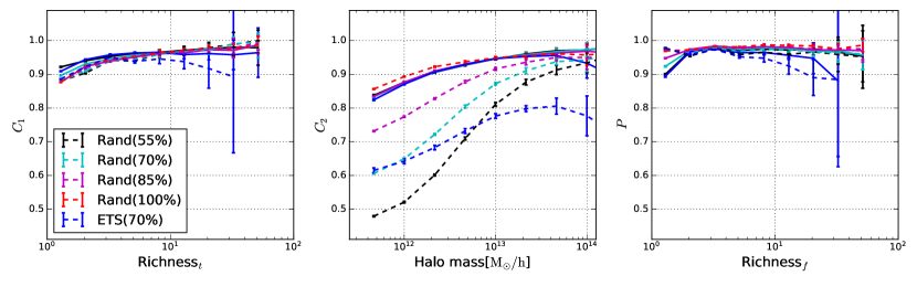
Figure 1: Performance comparison under MCM scheme with and without photometric data. Solid lines are results with photometric data while dashed lines use only spectroscopic data. Error bars are the standard deviations among 20 different mocks.

The good performance of the FoF group finder in terms of $C_{1}$ and $P$ indicates that the group finder is able to correctly identify most of the galaxy systems that are contained in the spectroscopic sample. Thus, the low $C_{2}$ values for cases of low sampling rates must be due to the missing of group systems in the spectroscopic sample, caused by incomplete sampling of the survey. In order to find these lost systems, we make use of information from the parent photometric sample. As mentioned in § 2, we apply the RFC to identify two kinds of lost central galaxies from the photometric sample: the group central and the isolated central.

To determine if a photometric galaxy is a group central, or an isolated central, or neither of the two, we characterize the relationship between the photometric galaxy and the spectroscopic groups around it. As described in § 2.2, we do this by determining both the hyper-parameters for RFC and $n_{g}$, the number of spectroscopic groups around the galaxy in question.

To find the optimal hyper-parameters of the RFC, we employ the $n$-fold cross-validation method. First, we randomly divide the photometric sample into $n$ sub-samples with an equal number of galaxies. We then train the model on $n-1$ sub-samples and make a prediction for the remaining one to test the performance. This process is repeated for each of the $n$ sub-samples. Here we choose $n=5$. We use the following set of quantities to describe the goodness of the prediction:

• $C_{\rm iso}$: Completeness of isolated centrals, defined as the fraction of isolated centrals that are correctly identified among all the isolated centrals in the photometric sample;

• $P_{\rm iso}$: Purity of isolated centrals, defined as the fraction of isolated centrals which are correctly identified among all the found isolated centrals;

• $C_{\rm grp}$: Completeness of group centrals, defined as the fraction of group centrals correctly identified among all group centrals, where a group central is the central of a group with at least one galaxy in the spectroscopic sample;

• $P_{\rm grp}$: Purity of group centrals, defined as the fraction of group centrals correctly identified among all the identified group centrals.

The hyper-parameters are chosen to achieve a balance among the above four quantities. Specifically, we optimize the values of the hyper-parameters by maximizing the quantity, $g$, defined as

$$g=C_{\rm iso}\cdot P_{\rm iso}\cdot C_{\rm grp}\cdot P_{\rm grp}$$ (10)

We find that the $g$ index is not sensitive to the exact values of the hyper parameters, so we will use the set of hyper-parameters given in Table 4 for different cases of redshift sampling. We also find that $n_{g}=3$ is sufficient for our purpose, independent of the redshift sampling.

Using the updated group catalog that incorporates photometric data, we plot the performance of the MCM scheme in Fig. 1. It can be seen that the main improvement is in the $C_{2}$ index at the low-mass end. This happens because most of the isolated centrals that are lost in the spectroscopic sample are now found in the photometric data. In addition, the missed massive groups in the ETS(70%) case can also be identified from the photometric data. There is, however, a noticeable decline in the purity at ${\rm Richness}_{f}=1$, since not all the isolated centrals identified from the photometric data are true centrals.

4.4 Assigning Halo Masses to Groups

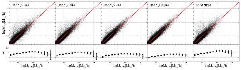
Figure 2: Upper panels: the scatter plot between the predicted halo mass and the true halo mass. Lower panel: the standard deviation in the true halo mass for a given predicted halo mass, with error bar showing the variance among 20 mocks.

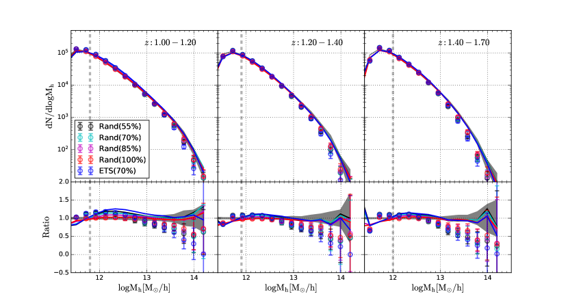
Figure 3: Halo mass functions in three redshift bins. The circle in upper panels are the halo mass functions of groups identified from samples of different redshift samplings, with error bars representing the variance among 20 mocks. The solid lines are means of the distribution for $\rm M_{h,samp}$. The shaded areas are the mass functions of simulated halos used to construct the mock catalogs, with the width indicating the variance among 20 mocks. The vertical dashed lines indicate masses below which the halo samples become incomplete. The lower panel shows the ratio of halo mass distribution obtained from the identified groups to that of the simulated halos.

Galaxies are formed and evolved in dark matter halos, and so the total stellar mass and number of member galaxies in a host halo are expected to be related to the dark matter mass of the host halo. Thus, it is possible to infer the halo mass of a group from the galaxies it contains. In this subsection, we apply the Random Forest Regressor (RFR), which is similar to the RFC, to infer the host halo mass for each of the identified galaxy groups (see Man et al., 2019, for a recent application of the RFR in this regard). The RFR is different from RFC in two ways. First, instead of the Gini impurity, RFR partitions the feature space to minimize the mean squared error (MSE), defined as

$${\rm MSE}=\sum_{j=1}^{|\mathcal{D}_{\rm bts,L}|}\left(y_{j}-\bar{y}_{\rm L}\right)+\sum_{j=1}^{|\mathcal{D}_{\rm bts,R}|}\left(y_{j}-\bar{y}_{\rm R}\right)$$ (11)

where $|\mathcal{D}_{\rm bts,L}|$ and $|\mathcal{D}_{\rm bts,R}|$ are the sizes of the two sub-samples at a node, $y_{j}$ is the $j$-th target value, and $\bar{y}_{\rm L}$ and $\bar{y}_{\rm R}$ are the means of the target values in the tow sub-samples. Second, the target value for each leaf is chosen to be the mean target value of the training sample in each leaf, rather than the mode. We use the following features from both the spectroscopic and photometric data to infer the halo mass:

1. ${\rm M_{*,tot}}$: the total stellar mass;

2. ${\rm M_{*,c}}$: the stellar mass of the central galaxy;

3. ${\rm N_{\rm tot}}$: the group richness, which is the total number of member galaxies (both spectroscopic and photometric);

4. ${\rm\sigma_{G}}$: velocity dispersion estimated using the gapper algorithm (Beers et al., 1990),

   $$\sigma_{G}={\sqrt{\pi}\over N(N-1)}\sum_{i=1}^{N-1}i(N-i)(v_{i+1}-v_{i})$$ (12)

   where $v_{i}=cz_{i}/(1+z_{\rm grp})$, with $v_{1}\leq v_{2}\leq...\leq v_{N}$, are the velocities of spectroscopic members, $z_{\rm grp}$ is the mean of $z_{i}$, and $N$ is the number of spectroscopic members. We set $\sigma_{G}=-1$ for systems with $N<2$.

5. ${\rm group~{}tag}$: which is equal to $0$ for a pure spectroscopic group, $1$ for a group with photometric central and spectroscopic members, and $2$ for an isolated photometric central;

6. ${\rm Redshift}$: group redshift, defined to be the photometric redshift of the central for groups that contain only a single photometric central, and to be the mean redshift of spectroscopic members for other groups;

7. ${\rm\log[M_{*,enc}(<5Mpc/h)-M_{*,tot}]}$: where $\rm M_{*,enc}(<5Mpc/h)$ is the total stellar mass of galaxies whose projected distance to the group center (defined by the sky position of the central and the redshift of the group) is smaller than 5 Mpc/h and the redshift difference (using spectral $z$ and photo-$z$ for spectroscopic and photometric galaxies, respectively) is smaller than 3$\sigma_{z,\rm phot}(1+z)$;

8. ${\rm\log[M_{*,enc}(<10Mpc/h)-M_{*,tot}]}$: similar to quantity defined above, except the projected distance to the group is smaller than 10Mpc/h.

As shown in the appendix, the information about halo mass is dominated by the first four features.

The hyper-parameters are tuned to minimize the mean squared error of the halo mass. Here we employ the $n$-fold cross-validation method as in § 4.3. The optimal values of the hyper-parameters are almost the same for different cases. We thus use the same set of values as given in Table 5 for cases of different redshift samplings.

Table 5: Adopted hyper-parameters for Random Forest Regressor in halo mass calibration

Hyper-parameter	Value
n_estimators	30
min_samples_split	30
max_features	3

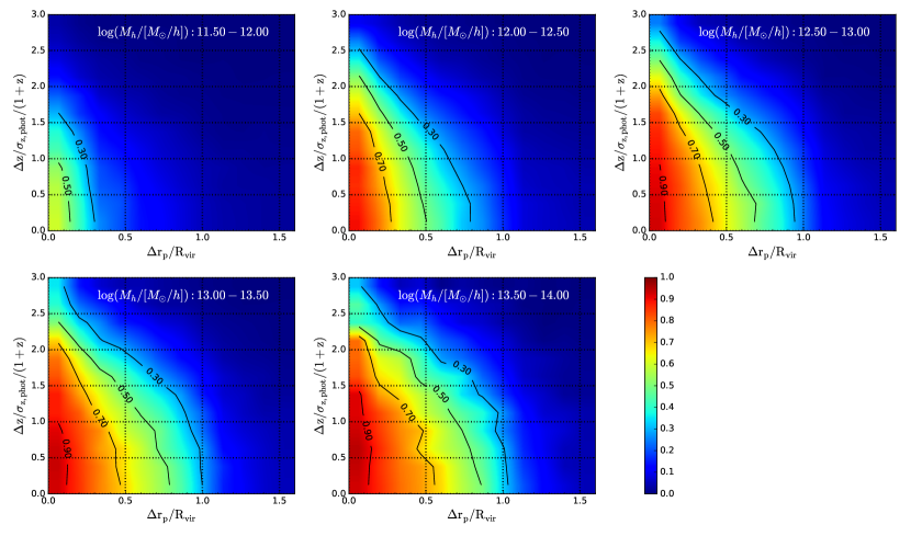
Figure 4: Fraction of true members as a function of $\Delta r_{p}$ and $\Delta z$ to the central galaxy. The figure is for Rand(55%).

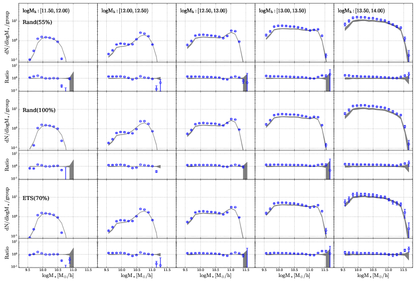
Figure 5: Conditional stellar mass functions in five halo mass bins obtained from samples of different redshift sampling rates. Blue circles are obtained from identified groups with error bars representing variation in 20 mocks (see text). And gray regions are obtained from model galaxies in simulated halos, with width represents the variance among 20 mocks. We also plot the ratio of the measurements to the mean value of the CSMF of model galaxies in simulated halos in the small panels.

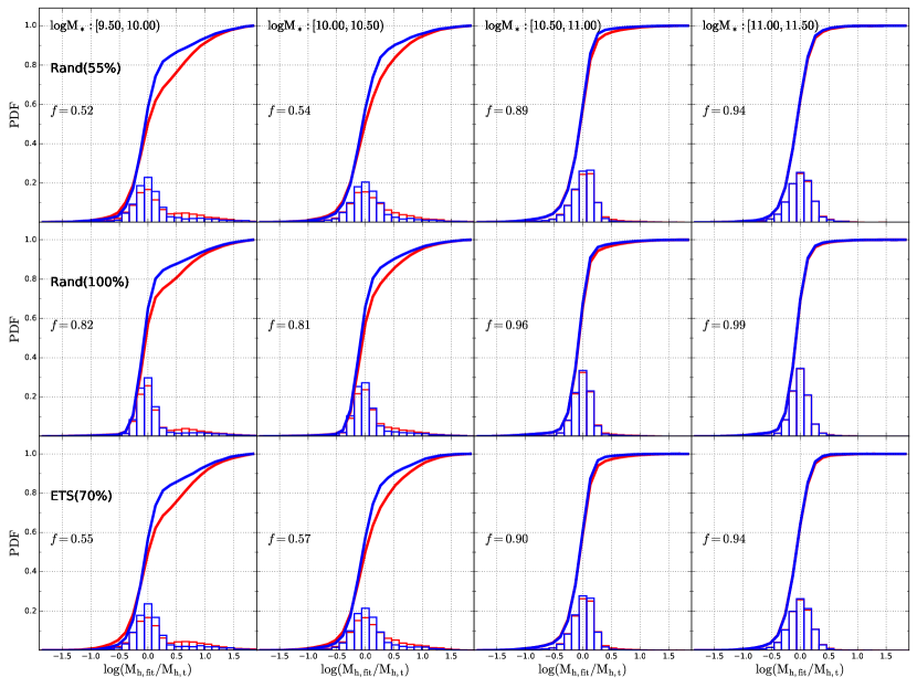
Figure 6: Blue histograms: distribution of $\rm\log(M_{h,fit}/M_{h,t})$ for galaxies with $\rm M_{h,fit}>10^{12}M_{\odot}/h$; Red histograms: distribution of $\rm\log(M_{h,fit}/M_{h,t})$ for galaxies with $\rm\log(M_{h,fit}h/M_{\odot})>12$, and with $\rm\Delta r_{p}/R_{vir}<1.0$ and $\Delta v/\rm V_{vir}<2.0$ (see text). The solid lines are the corresponding accumulated distribution. The $f$ indicates the number ratio of galaxies in the blue histogram with that in the red.

We use all the 20 mock catalogs to check the performance of the halo mass prediction. For each mock catalog, we use five other mock catalogs to train the RFR and to predict the results for the mock in question. The performance of the halo mass prediction is quantified by the discrepancy between the true halo mass, $\rm M_{h,t}$, and the predicted (fitted) halo mass, $\rm M_{h,fit}$.

In Fig. 2 we plot the relation between $\rm M_{h,t}$ and $\rm M_{h,fit}$ (upper panels) and the standard deviation of $\rm\log(M_{h,fit}/M_{h,t})$ (lower panels), for cases of different redshift sampling. For the case of 100% redshift sampling, the standard deviation ranges from 0.1 dex to 0.2 dex over the halo mass range from $\rm\sim 10^{11}M_{\odot}/h$ to $\rm\sim 10^{14}M_{\odot}/h$. This is similar to the result in Lim et al. (2017) for the SDSS galaxy sample using the halo-based group finder. For the cases of random sampling, the standard deviation at given halo mass increases with decreasing sampling rate, reaching a range between 0.15 dex to 0.22 dex for the sampling rate of 55%. In the case of ETS(70%), the overall performance is slightly worse than that of Rand(70%), particularly at the massive end ($>10^{13}M_{\odot}/h$). This can be understood as follows: due to fiber collisions the effective sampling rate is a decreasing function of galaxy target number density, leading to relatively low sampling rates for massive systems which are located in high-density regions. In ETS(70%) the effective sampling rate is only about 30% – 40% at halo masses above $\sim 10^{13}M_{\odot}/h$. As a result, many of the member galaxies in a massive group only have photometric redshifts and cannot be assigned to the group reliably. In addition, for cases with low sampling rates and for ETS(70%), there are outliers at the low-mass end, caused by groups that can be identified but their halo masses are poorly predicted owing to the missing of member galaxies in the spectroscopic sample.

The distribution of the predicted halo mass, $\rm M_{h,fit}$, is presented in Fig. 3 for three successive redshift intervals over $1<z<1.7$, in comparison with the halo mass functions obtained directly from the simulation used to construct the mock catalogs. It is obvious that the halo mass distribution is under-estimated to varying degree at the massive end ($>10^{13}M_{\odot}/h$), even for Rand(100%). This is expected, because our halo mass estimate is optimized for each selected group to have an estimated mass ($\rm M_{h,fit}$) that best match the true mass ($\rm M_{h,t}$), and because there is scatter in the true halo mass for a given estimated mass (see Fig. 2). To take into account the effects of such scatter, we introduce a random variable, $\rm M_{h,samp}$, defined as

$$\rm M_{\rm h,samp}=M_{\rm h,fit}+{\rm Norm}[0,~{}\sigma(M_{\rm h,fit})]$$ (13)

where $\rm Norm[0,~{}\sigma(M_{h,fit})]$ is a random number generated from a normal distribution with zero mean and a standard deviation, $\rm\sigma(M_{h,fit})$, as inferred from Fig. 2. To estimate a statistical quantity, $s$, using a set of halo masses, $\{{\rm M_{h,fit}}\}$, we first generate a set of halo masses, denoted by $\{{\rm M_{h,samp}}\}_{i}$, using Eq.(13), and repeat the process $N_{\rm samp}$ times. Our estimate for $s$ is

$$s_{\rm samp}={1\over N_{\rm samp}}\sum_{i=1}^{N_{\rm samp}}s(\{{\rm M_{h,samp}}\}_{i}).$$ (14)

The average distribution of $M_{\rm h,samp}$, obtained using $N_{\rm samp}=30$, is calculated in this way and plotted in Fig. 3 as the corresponding solid line for each of the cases. As one can see, the distribution of $M_{\rm h,samp}$ matches well the true halo mass function in the simulation for all cases, demonstrating again that the group sample selected by our group finder is quite complete and unbiased in the mass distribution. Note that due to the magnitude limit in our mock galaxy sample, the halo sample selected is incomplete at the low-mass end. A halo mass limit, below which the incompleteness becomes significant is indicated by the vertical dashed line in Fig. 3. This limit is defined as the mass below which the amplitude of the estimated mass function deviates from the halo mass function given by the original simulation by more than 0.05 dex.

4.5 Group memberships

The tests presented above are at the level of groups, based on group completeness and purity, and on halo mass assignments. In this subsection we will test our group finder at the level of group members. We first consider the conditional stellar mass function (CSMF) of member galaxies in halos of a given mass, which is defined as the average number of member galaxies in these groups as a function of the stellar mass of galaxies.

In order to account for redshift sampling effects, we need to include photometric galaxies around a group in a probabilistic way when calculating the CSMF. Here we employ a method similar to that proposed by Knobel et al. (2009), which consists of the following steps:

1. Construct the map of the fraction of true members: Using the mock catalog, we calculate the fraction of true members among all the photometric galaxies, excluding group centrals and isolated centrals, around spectroscopic groups (those identified from spectroscopic galaxies with spectroscopic or photometric centrals) with given halo mass, in bins of the redshift difference, $\Delta z/\sigma_{\rm z,phot}/(1+z)$, and the projected separation, $\Delta r_{p}/R_{\rm vir}$. As an example, Fig. 4 shows the map of the fraction for the case of Rand(55%).

2. Assign membership probability: After running the group finding pipeline, each photometric galaxy, $i$, that has not been identified as an isolated central or a group central, will be assigned to a spectroscopic group, $J$, in its neighborhood with a probability, $p_{i\rightarrow J}$, inferred from the fraction map constructed in previous step, based on the redshift difference and projected distance to the group. We note that each photometric galaxy, $i$, can be assigned to several groups around in a probabilistic manner.

3. Regulate the probability: To ensure the summation of the probabilities for a photometric galaxy to belong to all of its neighboring spectroscopic groups and to be in the field is equal to one, we regulate the probability as (Knobel et al., 2012a)

   $$\tilde{p}_{i\rightarrow J}=p_{i\rightarrow J}\times{{1-p_{\rm field}}\over\sum_{J}p_{i\rightarrow J}},~{}~{}~{}{\rm with}~{}~{}p_{\rm field}=\prod_{J}(1-p_{i\rightarrow J})$$ (15)

Finally, we estimate the CSMF as

$$\Phi(M_{*}|M_{\rm h,l},~{}M_{\rm h,u})={\sum_{i}\sum_{J}\tilde{p}_{i\rightarrow J}\over N_{\rm G}\Delta M_{*}}\,,$$ (16)

where the summation on $i$ runs over all the galaxies whose stellar masses satisfy $M_{*}-\Delta M_{*}/2\leq M_{*,i}<M_{*}+\Delta M_{*}/2$, and summation on $J$ runs over all $N_{\rm G}$ spectroscopic groups whose halo masses satisfy $M_{\rm h,l}\leq M_{*,j}<M_{\rm h,u}$. For each spectroscopic galaxy or group central, $i$, we set $\tilde{p}_{i\rightarrow J}=1$ if it belongs to group $J$, and $\tilde{p}_{i\rightarrow J}=0$ otherwise.

The CSMFs estimated in this way are plotted in Fig. 5 in five halo mass bins (blue circles) with error bars representing the variance between the 20 mock catalogs, in comparison with the CSMFs obtained directly from the member galaxies of dark halos in the simulation (gray shaded regions). Here we only show results for three sampling cases since the results of the other two cases fall in between Rand(55%) and Rand(100%). As one can see, the CSMFs obtained from the identified galaxy groups match well the input mock catalog. However, we overestimate slightly the amplitudes of the CSMFs at the low-mass end where the mass functions are dominated by satellite galaxies. This happens because we have adopted the same set of FoF parameters calibrated with ETS(70%), which is slightly different from the optimal set for other cases of redshift sampling. The amplitudes of the CSMFs obtained from galaxy groups are also reduced if $M_{\rm h,samp}$ is used instead of $M_{\rm h,fit}$.

Next, we consider the host halo mass distribution for spectroscopic galaxies in four stellar mass bins. Different from the halo mass comparison for groups, host halo mass distribution for galaxies are affected by membership assignment error, and thus provides a better quantification of halo mass uncertainties when halo masses are used as an environment indicator for individual galaxies. The differential and accumulated distributions of $\rm\log(M_{h,fit}/M_{h,t})$ for all the spectroscopic galaxies in $\rm M_{h,fit}>10^{12}M_{\odot}/h$ are presented in Fig. 6 as the red histograms and red solid lines, respectively. We note that there is a small tail in the distribution at high $\rm\log(M_{h,fit}/M_{h,t})$ for low stellar mass bins. This is produced by galaxies which are hosted by low-mass halos around massive groups but identified as satellites of the massive groups (interlopers) by the group finder. To reduce the effects of these interlopers, one can trim the galaxy sample by requiring the galaxies to satisfy the following criteria:

$$\Delta{\rm r_{p}} <\alpha_{r}R_{\rm vir}$$ (17)

$$\Delta v <\alpha_{v}V_{\rm vir}$$ (18)

where $\Delta\rm r_{p}$ is the projected distance of a galaxy to the group center, and $\Delta v$ is the line of sight velocity of the galaxy relative to the group center. Here the group center is defined as the projected position of central galaxy and mean redshift of spectroscopic members. $R_{\rm vir}$ and $V_{\rm vir}$ are respectively the virial radius and virial velocity corresponding to the halo mass of the group $M_{\rm h,fit}$. Blue histograms and blue solid lines in Fig. 6 show the results for the case where $\alpha_{r}=1$ and $\alpha_{v}=2$. In each panel $f$ indicates the fraction of galaxies in the parent (untrimmed) sample that are kept after trimming. As expected, the tail of the $\rm\log(M_{h,fit}/M_{h,t})$ distribution is largely reduced, especially at low stellar masses. Indeed, using $\alpha_{r}=1$ and $\alpha_{v}=1$ will get rid of the tail almost completely. However, the value of $f$ is quite low for low-mass galaxies and is lower when a more restrictive limit is applied, indicating that many of the interlopers are located in the outer parts of halos. The fact that a substantial fraction of low-mass galaxies are located beyond $R_{\rm vir}$ and have relative velocities larger than $V_{\rm vir}$ is because the groups identified by the group finder are usually non-spherical, particularly in high density regions. Note that the $\rm\log(M_{h,fit}/M_{h,t})$ distributions shown in Fig. 6 are weighted by the number of galaxies in halos, so that the extended tails in the distributions are dominated by a small number of systems in high density regions where the contamination by interlopers is severe. In any case, for investigations where purity of member galaxies is crucial, one should adopt restrictive limits on $\Delta{\rm r_{p}}$ and $\Delta v$ to reduce the contamination by interlopers.

5 The application to the zCOSMOS-bright sample

The zCOSMOS-bright is a spectroscopic galaxy survey obtained with the ESO VLT (Lilly et al., 2007, 2009). It contains about 20,000 galaxies with $15.0\leq I_{\rm AB}\leq 22.5$ in an area of about 1.7deg² in the COSMOS field and in the redshift range $0.1\lesssim z\lesssim 1.2$. The redshift completeness, defined as the product of the redshift sampling rate and the redshift success rate (Knobel et al., 2012a), is $\sim 48\%$ in the full zCOSMOS-bright area and $\sim 56\%$ in the central region. As discussed in de la Torre et al. (2011), the sampling effects for zCOSMOS can be modeled as a function of the right ascension (RA) and redshift. As an application of our group finding pipeline, we will identify galaxy groups in the central region of the COSMOS area using both spectroscopic and photometric galaxies at $0.1\leq z\leq 1.0$.

5.1 Tests with zCOSMOS-bright mock samples

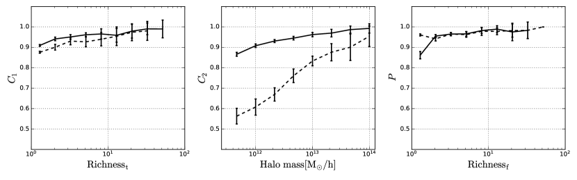
Figure 7: Performance of our group finder on the zCOSMOS-bright mock catalog in terms of $C_{1}$, $C_{2}$ and $P$ (see Table 2 for definitions). The dashed lines are for the spectroscopic only sample and the solid lines are the performance including photometric data. Error bars show the standard deviations among 20 different mock samples.

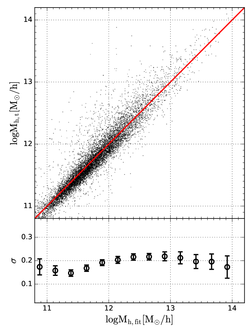
Figure 8: Performance of the group finder on halo mass for zCOSMOS-bright mock catalogs, shown as the relationship between the true halo mass, $M_{\rm h,t}$, and the predicted halo mass, $M_{\rm h,fit}$. The standard deviations of true halo halo mass for a given predicted mass are shown in the lower panel as circles, with error bars representing the variances among 20 mock samples.

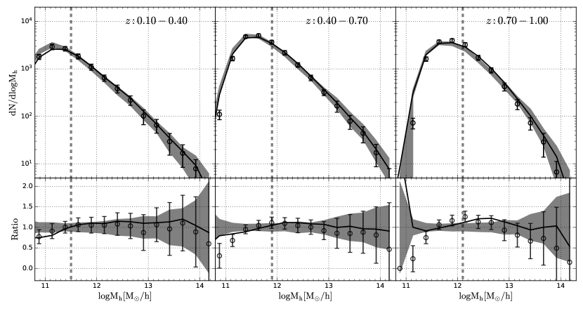
Figure 9: Halo mass functions for identified groups in zCOSMOS-bright mock samples. The Grey shaded regions are the ranges covered by the halo mass distribution by the 20 mock samples. The data points with error bars are for identified groups with estimated halo masses. The solid lines are for $\rm M_{h,samp}$. The vertical dashed lines are the mass limits reached by the catalog. The lower panels show the same functions but normalized by the mean of the 20 mock samples.

Table 6: Optimal parameters of friend-of-friend group finder in the central region for zCOSMOS-bright survey.

Parameters	$b$	$l\_{\rm max}$(Mpc/h)	$R$
Values	0.08	0.30	17.00

To quantify the performance of our group finding pipeline on the zCOSMOS-bright like surveys, we constructed 20 different mock catalogs to mimic the selection effects and incompleteness for the central region of the real zCOSMOS-bright survey in the redshift range of $0.1\leq z\leq 1.0$ (Meng et al., 2020).

The group level performance of our group finder for the zCOSMOS-bright mock samples, which uses the optimal parameters listed in Table 6, is shown in Fig. 7. The dashed lines are based on spectroscopic-only galaxies, while solid lines use both spectroscopic and photometric galaxies. Similar to the results presented above, our group finder performs well in terms of both $C_{1}$ and $P$ (both $\gtrsim 90\%$). A large deficit in the $C_{2}$ index is observed when only spectroscopic galaxies are used, especially for low mass halos, but the inclusion of photometric galaxies improves the performance dramatically.

We also estimate the halo masses using the RFR as described above, and the performance is shown in Fig. 8. Over the entire mass range from $\rm\sim 10^{11}M_{\odot}/h$ to $\rm\sim 10^{14}M_{\odot}/h$, the standard deviation of the estimated halo mass is about 0.2 dex. The estimated halo mass functions are shown in Fig. 9 as data points with error bars, in comparison with those obtained directly from 20 mock samples (gray regions). The black solid lines are the average distribution function of $\rm M_{h,samp}$ among 30 random samples obtained using equation (13). For comparison, the mass limit for completeness is indicated as vertical dashed line in each panel. As one can see, the input halo mass functions can be well recovered; the large scatter at the massive end among different mock samples reflects the level of the cosmic variance expected for a sample like zCOSMOS-bright.

5.2 The zCOSMOS-bright group catalog

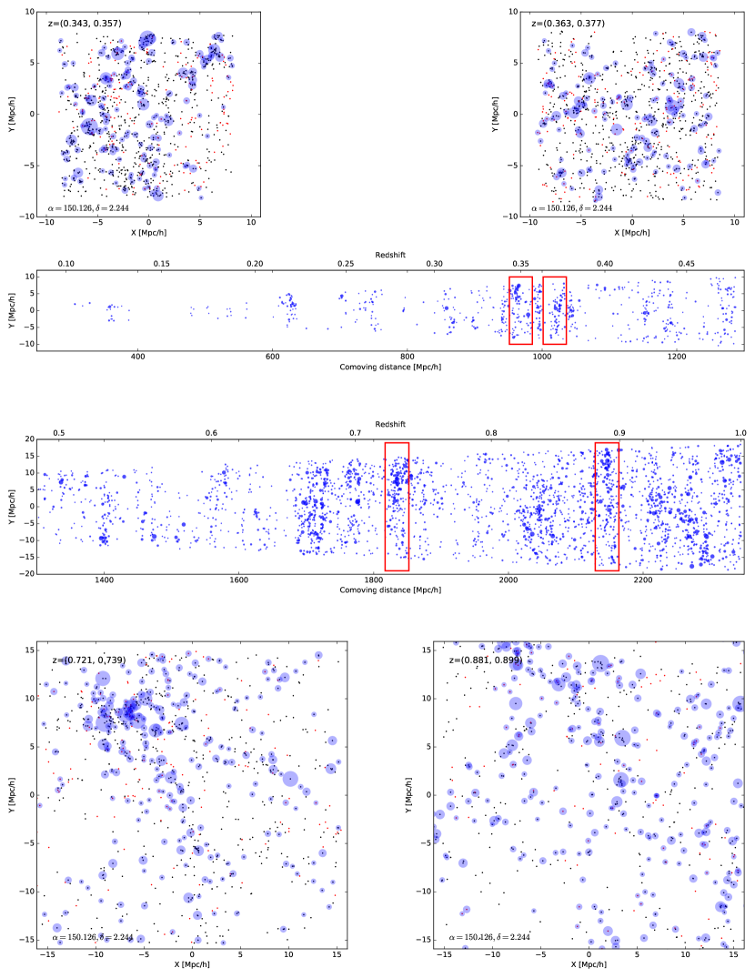
Figure 10: The projected distributions of galaxies and identified groups in four redshift slices. The black dots are spectroscopic galaxies and the red dots are photometric galaxies. The blue circles represent the galaxy groups with $\rm M_{h}>10^{12}M_{\odot}/h$), with radius proportional to the halo radius.

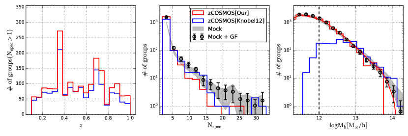
Figure 11: Comparison between our group catalog with that of Knobel et al. (2012a). Left panel: redshift distribution; Middle panel: richness distribution; Right panel: halo mass distribution. Our results are shown by red histograms while those of Knobel et al. (2012a) by blue histograms. The red solid curve in the right panel is the distribution of $\rm M_{h,samp}$ obtained from our catalog. Circles with error bars are the mean and variance obtained by applying our group finder to the 20 zCOSMOS-bright mock catalogs, while the grey regions cover the ranges obtained directly from the 20 mock catalogs. The vertical dashed line in the right panel indicates the completeness limit. Note that the halo masses are available only for groups that contain at least 2 spectroscopic members in the catalog of Knobel et al. (2012a).

We have applied our group finder to zCOSMOS-bright galaxies at $0.1\leq z\leq 1.0$ in the central region that covers $\sim$1 deg². We also excluded unreliable redshift measurements tagged as 0, 1.1, 2.1 and 9.1 (Lilly et al., 2009). The final spectroscopic sample contains 11,489 galaxies. The photometric data used is adopted from the parent photometric sample, constructed from Laigle et al. (2016) by Meng et al. (2020). The spectroscopic groups are identified using the FoF group finder with optimal parameters calibrated by the mock samples (see Table 6). Starting from the spectroscopic groups, we identify both isolated centrals and group centrals that are missed in the spectroscopic sample based on the parent photometric sample, using the RFC method described in § 2.2. Finally, we calibrate the halo masses for the final group catalog using the RFR described in § 4.4.

Fig. 10 shows the spatial distribution of the identified groups in the $(Y,Z)$ plane (the two middle panels) where $Z$ is in the radial (redshift) direction, and $Y$ is one of the two directions perpendicular to $Z$. As illustrations, the four square panels in the upper and lower rows show the distribution in the $X$-$Y$ plane for groups in four redshift slices with $\Delta z=0.01(1+z)$, as indicated by the four red rectangles. Only groups with $\rm M_{h}\geq 10^{12}M_{\odot}/h$ are plotted, and each of them is shown as a blue circle with radius proportional to its halo radius. For comparison, we also show spectroscopic galaxies as black points, and photometric galaxies as red points. We can see clearly, as expected, that galaxy groups trace the large-scale structure in the galaxy distribution, and that massive groups reside preferentially in high density regions.

We plot the redshift ($z$) distribution of our identified groups in Fig. 11, in comparison with that obtained by Knobel et al. (2012a). Despite of the different methods used to identify galaxy groups, the two distributions match well with each other. Fig. 11 also shows the richness and halo mass distributions of our group catalog, again in comparison with those obtained from the catalog of Knobel et al. (2012a). Both group catalogs give a similar distribution in the richness of spectroscopic members. This is expected, as we are using a similar method to identify groups in the spectroscopic sample. However, our catalog contains many more low-mass systems, because we include isolated systems and our halo mass estimator provides reliable mass estimates even for low-mass halos. There is also discrepancy between the two catalogs at the massive end, where our group catalog contains smaller number of groups. We believe that this owes to the galaxy number density re-calibration used by Knobel et al. (2012a), as described below. As a demonstration, the circles with error bars in Fig. 11 show the result obtained by applying our group finder to the 20 zCOSMOS-bright mock catalogs, in comparison to that obtained directly from the mock catalogs, shown by the grey regions. The fact that these two results match well with each other indicates that our group finder is reliable. The discrepancy between our zCOSMOS-bright results and the mock results then suggests that the zCOSMOS-bright is not a fair sample, particularly for massive groups.

Knobel et al. (2012a) published a galaxy group catalog based on the spectroscopic galaxies from zCOSMOS 20k, using the FoF group finding algorithm in a "multi-run scheme", and using photometric galaxies to make improvements on group membership and group center. They calibrated their FoF parameters and halo mass estimator using mock catalogs that are scaled so that the average density distribution of galaxies matches that in the real sample. Thus, their results are, in a sense, corrected for cosmic variance. This may explain why their group mass function matches the expected mass function better at the massive end (see the right panel of Fig. 11). In this paper, we decide to provide a group catalog that is based on the data itself, while leaving the correction for the cosmic variance to specific applications of the catalog. In addition, our group finding algorithm is different from that of Knobel et al. (2012a) in the following aspects. First, we use the state of the art random forest algorithm to incorporate photometric galaxies and to improve the completeness and purity of our group catalog. Second, we use a halo mass estimator, calibrated with realistic mock catalogs and the random forest method, so that we are able to provide accurate halo mass estimates for groups over a large mass range.

5.3 Catalog contents

The group catalog constructed and the galaxy sample used for the construction are available through https://github.com/wkcosmology/zCOSMOS-bright_group_catalog. The group catalog lists the properties of individual groups, while the galaxy sample provides information about individual galaxies as well as their links to groups. In what follows we explain the contents of these catalogs in more detail.

5.4 The group catalog

The following items are provided for individual groups.
Column (1) groupID: a unique ID of each group in the group catalog;
Column (2) cenID: galaxy ID of the central galaxy of a group;
Column (3) cenID2015: central galaxy ID in Laigle et al. (2016);
Column (4) RA_avg: Right Ascension (J2000) of the group center in degrees, defined as the average RA of member galaxies weighted by the stellar mass
Column (5) Dec_avg: Declination (J2000) of the group center in degrees, defined as the average Dec of member galaxies weighted by the stellar mass
Column (6) z_avg: redshift of the group, defined as the average redshift of member galaxies with spectroscopic redshift weighted by the stellar mass
Column (7) HaloMass: 10-based logarithm of the halo mass of a group in units of $\rm M_{\odot}$;
Column (8) GroupTag: 0 for groups with only spectroscopic members, 1 for groups with photometric central and spectroscopic member, and 2 for groups with only one photometric member; Column (9) Richness: number of member galaxies in a group;

5.5 The galaxy catalog

The following items are provided for individual galaxies
Column (1) ID: unique ID of galaxies, which can be used to match galaxies across the galaxy and group catalogs;
Column (2) surveyID: ID of galaxies from the original survey data release. This can be used to match galaxies across our catalogs and the original survey data release;
Column (3) ID2015: galaxy id in Laigle et al. (2016);
Column (4) groupID: ID of the group of which a galaxy is a member;
Column (5) RA: right ascension (J2000) in degrees;
Column (6) Dec: declination (J2000) in degrees;
Column (7) z: redshift
Column (8) StellarMass: 10-based logarithm of the galaxy in units of $\rm M_{\odot}$;
Column (9) tag: 1 for central, 0 for satellite;
Column (10) CC: redshift confidence class, $-1$ for photometric redshift, others see Lilly et al. (2007).

6 Summary

In this paper, we have developed a group finder that is suitable for identifying galaxy groups from incomplete redshift samples combined with photometric data. A machine learning method is adopted to assign halo masses to identified groups. To test the impact of redshift sampling effects, we have constructed realistic mock samples with different redshift sampling schemes and applied our group finder to them. Our main results are summarized as follows.

1. We find that our modified version of the FoF group finder based on a local, incompleteness-corrected linking-length can identify most of the galaxy systems correctly from an incomplete spectroscopic sample (Fig. 1), even with a sampling rate that is as low as 55% and is spatially in-homogeneous.

2. We find that an incomplete redshift sampling can cause the loss of galaxy groups from a spectroscopic sample. For random sampling cases, many of the low-mass groups are lost although the massive ones can still be identified due to their high richness. However, with realistic fiber assignments, such as the one to be adopted by the up-coming PFS galaxy survey, massive galaxy systems can also be missed because of the lower sampling rates in higher density regions caused by fiber collisions (Fig. 1).

3. With the use of the state-of-the-art random forest algorithm, we find that it is possible to retrieve most of the lost groups using a combination of spectroscopic and photometric data. The final completeness and purity that can be achieved can reach to $\gtrsim 85\%$ (Fig. 1) even for a sampling rate as low as 55% and for an in-homogeneous sampling.

4. We calibrate the host halo mass for identified galaxy groups with the random forest regressor algorithm. We find that the estimated halo masses are un-biased relative to the true masses, with an uncertainty of about 0.15 – 0.25 dex over a wide range of halo masses (Fig. 2). The estimated halo mass distribution matches the input mass function well after the statistical bias caused by the mass uncertainty is taken into account.

5. We find that the conditional stellar mass functions of galaxies in halos of different masses can be well recovered from the identified groups with estimated halo masses (Fig. 5).

6. We find that the groups identified by our group finder provide an accurate link between individual galaxies and the masses of their host halos (Fig. 6). Although there are some interlopers with high $\rm\log(M_{h,fit}/M_{h,t})$, we have shown that these outliers can be eliminated by cutting out members in the outer parts of groups.

7. We have applied our group finding algorithm to the zCOSMOS-bright spectroscopic redshift survey and constructed a new catalog of galaxy groups in $0.1\leq z\leq 1.0$. Our tests using mock catalogs show that most of the galaxy groups are identified correctly (Fig. 7) with reliable halo masses (Fig. 8). Compared with the previous group catalog selected from the zCOSMOS-bright survey, our catalog is more complete, extending the halo mass range to much lower masses. Our halo mass estimates are reliable over the entire mass range covered by our catalog, as shown by our tests based on realistic mock catalogs.

Identifying galaxy groups from redshift surveys of galaxies plays an important role in connecting galaxies with the underlying dark matter distribution. Our results demonstrate clearly that such investigations can also be carried out for current and future high-$z$ spectroscopic surveys. This opens a new avenue to connect galaxies to their dark matter halos at high $z$, thereby to study galaxy evolution in different environments. Furthermore, the success of our method to construct highly complete group samples covering large halo mass ranges demonstrates that galaxy groups properly identified at high $z$ can be used to represent the dark halo population in the early universe. One can thus use them to reconstruct the cosmic density field and to study the large-scale structure in the early universe, as was done in low $z$ (Wang et al., 2009). One can also use the galaxy groups as tracers to investigate the properties of dark matter halos at high $z$ through, e.g., their gravitational lensing effects and Sunyaev–Zel’dovich effects.

Data availability

The data underlying this article will be shared on reasonable request to the corresponding author. The zCOSMOS-bright group catalog are available at https://github.com/wkcosmology/zCOSMOS-bright_group_catalog.

Appendix A The importance of different features used for halo mass estimate

We employ the RFR to predict the halo mass for galaxy groups (§4.4), using several group properties as input features. RFR also provides a way to quantify the contribution of each individual feature to the prediction in terms of feature importance. Recall that the random forest is assembled by many decision trees, each of which is constructed by iteratively bi-partitioning the sample into left and right children with one feature, and each bi-partition is to minimize a certain goal function (like Gini impurity for RFC, and the mean squared error for RFR). Heuristically, if a feature is always chosen to bi-partition the tree and the bi-partitions can dramatically decrease the goal function, this feature must be important in predicting the target value. The importance of feature-$i$ can thus be calculated for a decision tree though

$${\rm Imp}_{i}={\sum_{j:{\rm nodes~{}splitted~{}according~{}to~{}feature-}i}{\rm\Delta MSE}_{j}\over\sum_{j:{\rm all~{}nodes}}{\rm\Delta MSE}_{j}}$$ (19)

where the summation $j$ is for the internal nodes. The quantity ${\rm\Delta MSE}_{j}$ is the MSE decrement for each $j$-th internal node, defined as

$${\rm\Delta MSE}_{j} =\sum_{l}^{|\mathcal{D}_{j}|}(y_{l}-\bar{y}_{j})^{2}$$ (20)

$$-\sum_{l}^{|\mathcal{D}_{j,\rm L}|}(y_{l}-\bar{y}_{j,\rm L})^{2}-\sum_{l}^{|\mathcal{D}_{j,\rm R}|}(y_{l}-\bar{y}_{j,\rm R})^{2}$$ (21)

where $\bar{y}_{j}$ is the target mean of data points in node $j$; $\bar{y}_{j,\rm L}$ and $\bar{y}_{j,\rm R}$ are the target means for the left and right children, respectively; $|\mathcal{D}_{j}|$, $|\mathcal{D}_{j,\rm L}|$ and $|\mathcal{D}_{j,\rm R}|$ are the numbers of data points in node $j$ and in its left and right children, respectively. Fig. 12 shows the importance of different features adopted in the main text to determine the halo mass, with the total importance normalized to unity. As one can see, the total stellar mass, central stellar mass, richness and velocity dispersion are the four features dominating the contribution, while other features contribute little.

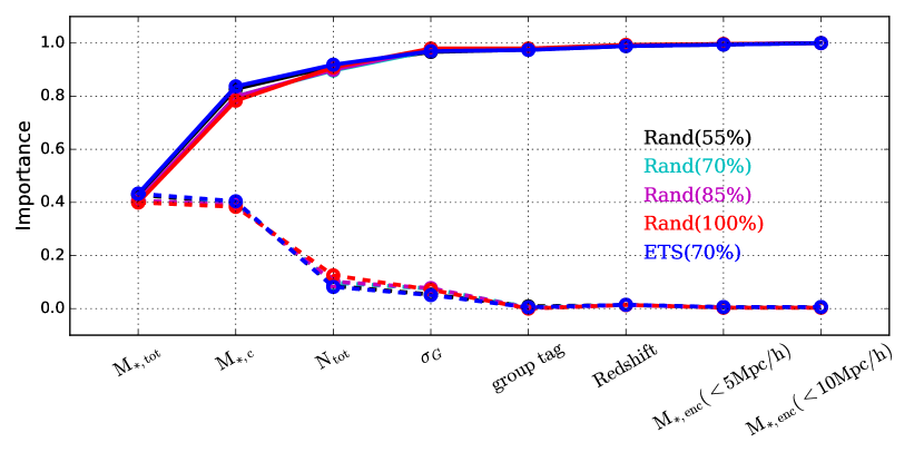
Figure 12: Feature importance (dashed lines) and the corresponding cumulative distribution (solid lines) for different sampling cases.

References

- Abell (1958) Abell G. O., 1958, The Astrophysical Journal Supplement Series, 3, 211
- Abell et al. (1989) Abell G. O., Corwin Jr. H. G., Olowin R. P., 1989, The Astrophysical Journal Supplement Series, 70, 1
- Aihara et al. (2018) Aihara H., et al., 2018, Publications of the Astronomical Society of Japan, 70
- Beers et al. (1990) Beers T. C., Flynn K., Gebhardt K., 1990, The Astronomical Journal, 100, 32
- Berlind et al. (2006) Berlind A. A., et al., 2006, The Astrophysical Journal Supplement Series, 167, 1
- Chen et al. (2019) Chen Y., Mo H. J., Li C., Wang H., Yang X., Zhou S., Zhang Y., 2019, The Astrophysical Journal, 872, 180
- Coil et al. (2006) Coil A. L., et al., 2006, The Astrophysical Journal, 638, 668
- Crook et al. (2007) Crook A. C., Huchra J. P., Martimbeau N., Masters K. L., Jarrett T., Macri L. M., 2007, The Astrophysical Journal, 655, 790
- Cucciati et al. (2010) Cucciati O., et al., 2010, Astronomy & Astrophysics, 520, A42
- Darvish et al. (2017) Darvish B., Mobasher B., Martin D. C., Sobral D., Scoville N., Stroe A., Hemmati S., Kartaltepe J., 2017, The Astrophysical Journal, 837, 16
- Davis et al. (1985) Davis M., Efstathiou G., Frenk C. S., White S. D., 1985, The Astrophysical Journal, 292, 371
- Dong et al. (2008) Dong F., Pierpaoli E., Gunn J. E., Wechsler R. H., 2008, The Astrophysical Journal, 676, 868
- Duarte & Mamon (2015) Duarte M., Mamon G. A., 2015, Monthly Notices of the Royal Astronomical Society, 453, 3849
- Dunkley et al. (2009) Dunkley J., et al., 2009, The Astrophysical Journal Supplement Series, 180, 306
- Eke et al. (2004) Eke V. R., et al., 2004, Monthly Notices of the Royal Astronomical Society, 348, 866
- Euclid Collaboration et al. (2019) Euclid Collaboration et al., 2019, Astronomy & Astrophysics, 627, A23
- Gerke et al. (2005) Gerke B. F., et al., 2005, The Astrophysical Journal, 625, 6
- Gerke et al. (2013) Gerke B. F., Wechsler R. H., Behroozi P. S., Cooper M. C., Yan R., Coil A. L., 2013, The Astrophysical Journal Supplement Series, 208, 1
- Gillis & Hudson (2011) Gillis B. R., Hudson M. J., 2011, Monthly Notices of the Royal Astronomical Society, 410, 13
- Goto (2005) Goto T., 2005, Monthly Notices of the Royal Astronomical Society, 359, 1415
- Guzzo et al. (2014) Guzzo L., et al., 2014, Astronomy & Astrophysics, 566, A108
- Han et al. (2015) Han J., et al., 2015, Monthly Notices of the Royal Astronomical Society, 446, 1356
- Huchra & Geller (1982) Huchra J. P., Geller M. J., 1982, The Astrophysical Journal, 257, 423
- Kawinwanichakij et al. (2016) Kawinwanichakij L., et al., 2016, The Astrophysical Journal, 817, 9
- Kepner et al. (1999) Kepner J., Fan X., Bahcall N., Gunn J., Lupton R., Xu G., 1999, The Astrophysical Journal, 517, 78
- Knobel et al. (2009) Knobel C., et al., 2009, The Astrophysical Journal, 697, 1842
- Knobel et al. (2012a) Knobel C., et al., 2012a, The Astrophysical Journal, 753, 121
- Knobel et al. (2012b) Knobel C., et al., 2012b, The Astrophysical Journal, 755, 48
- Knobel et al. (2015) Knobel C., Lilly S. J., Woo J., Kovač K., 2015, The Astrophysical Journal, 800, 24
- Laigle et al. (2016) Laigle C., et al., 2016, The Astrophysical Journal Supplement Series, 224, 24
- Lan et al. (2016) Lan T.-W., Ménard B., Mo H., 2016, Monthly Notices of the Royal Astronomical Society, 459, 3998
- Lavaux & Hudson (2011) Lavaux G., Hudson M. J., 2011, Monthly Notices of the Royal Astronomical Society, 416, 2840
- Le Fèvre et al. (2005) Le Fèvre O., et al., 2005, Astronomy & Astrophysics, 439, 845
- Li & Yee (2008) Li I. H., Yee H. K. C., 2008, The Astronomical Journal, 135, 809
- Li et al. (2011) Li R., Mo H. J., Fan Z., Bosch F. C. v. d., Yang X., 2011, Monthly Notices of the Royal Astronomical Society, 413, 3039
- Lilly et al. (2007) Lilly S. J., et al., 2007, The Astrophysical Journal Supplement Series, 172, 70
- Lilly et al. (2009) Lilly S. J., et al., 2009, The Astrophysical Journal Supplement Series, 184, 218
- Lim et al. (2017) Lim S., Mo H., Lu Y., Wang H., Yang X., 2017, Monthly Notices of the Royal Astronomical Society, 470, 2982
- Lim et al. (2018) Lim S. H., Mo H. J., Li R., Liu Y., Ma Y.-Z., Wang H., Yang X., 2018, The Astrophysical Journal, 854, 181
- Lim et al. (2020) Lim S., Mo H., Wang H., Yang X., 2020, The Astrophysical Journal, 889, 48
- Lu et al. (2014) Lu Z., Mo H. J., Lu Y., Katz N., Weinberg M. D., van den Bosch F. C., Yang X., 2014, Monthly Notices of the Royal Astronomical Society, 439, 1294–1312
- Lu et al. (2016) Lu Y., et al., 2016, The Astrophysical Journal, 832, 1
- Lubin et al. (2009) Lubin L. M., Gal R. R., Lemaux B. C., Kocevski D. D., Squires G. K., 2009, The Astronomical Journal, 137, 4867
- Luo et al. (2018) Luo W., et al., 2018, The Astrophysical Journal, 862, 4
- Man et al. (2019) Man Z.-y., Peng Y.-j., Shi J.-j., Kong X., Zhang C.-p., Dou J., Guo K.-x., 2019, arXiv.org
- Mandelbaum et al. (2006) Mandelbaum R., Seljak U., Cool R. J., Blanton M., Hirata C. M., Brinkmann J., 2006, Monthly Notices of the Royal Astronomical Society, 372, 758
- Marinoni et al. (2002) Marinoni C., Davis M., Newman J. A., Coil A. L., 2002, The Astrophysical Journal, 580, 122
- Maturi et al. (2019) Maturi M., Bellagamba F., Radovich M., Roncarelli M., Sereno M., Moscardini L., Bardelli S., Puddu E., 2019, Monthly Notices of the Royal Astronomical Society, 485, 498
- Meng et al. (2020) Meng J., Li C., Mo H., Chen Y., Wang K., 2020, arXiv:2008.13733 [astro-ph]
- Mo & White (1996) Mo H., White S. D., 1996, Monthly Notices of the Royal Astronomical Society, 282, 347
- Mo et al. (2010) Mo H., Van den Bosch F., White S., 2010, Galaxy formation and evolution. Cambridge University Press
- Muñoz-Cuartas et al. (2011) Muñoz-Cuartas J. C., Müller V., Forero-Romero J. E., 2011, Monthly Notices of the Royal Astronomical Society, 417, 1303
- Newman et al. (2013) Newman J. A., et al., 2013, The Astrophysical Journal Supplement Series, 208, 5
- Oguri et al. (2018) Oguri M., et al., 2018, Publications of the Astronomical Society of Japan, 70
- Pedregosa et al. (2011) Pedregosa F., et al., 2011, Journal of Machine Learning Research, 12, 2825
- Rodriguez et al. (2015) Rodriguez F., Merchán M., Sgró M. A., 2015, Astronomy & Astrophysics, 580, A86
- Tago et al. (2006) Tago E., Einasto J., Einasto M., Saar E., 2006, Astronomische Nachrichten, 327, 365
- Takada et al. (2014) Takada M., et al., 2014, Publications of the Astronomical Society of Japan, 66, R1
- Tinker et al. (2011) Tinker J., Wetzel A., Conroy C., 2011, arXiv.org, p. arXiv:1107.5046
- Tully (2015) Tully R. B., 2015, The Astronomical Journal, 149, 171
- Vikram et al. (2017) Vikram V., Lidz A., Jain B., 2017, Monthly Notices of the Royal Astronomical Society, p. stw3311
- Viola et al. (2015) Viola M., et al., 2015, Monthly Notices of the Royal Astronomical Society, 452, 3529
- Wang et al. (2009) Wang H., Mo H. J., Jing Y. P., Guo Y., van den Bosch F. C., Yang X., 2009, Monthly Notices of the Royal Astronomical Society, 394, 398–414
- Wang et al. (2016) Wang H., et al., 2016, The Astrophysical Journal, 831, 164
- Wang et al. (2018) Wang H., et al., 2018, The Astrophysical Journal, 852, 31
- Weinmann et al. (2006) Weinmann S. M., van den Bosch F. C., Yang X., Mo H. J., 2006, Monthly Notices of the Royal Astronomical Society, 366, 2
- Yang et al. (2005a) Yang X., Mo H., Van Den Bosch F. C., Jing Y., 2005a, Monthly Notices of the Royal Astronomical Society, 356, 1293
- Yang et al. (2005b) Yang X., Mo H. J., van den Bosch F. C., Weinmann S. M., Li C., Jing Y. P., 2005b, Monthly Notices of the Royal Astronomical Society, 362, 711
- Yang et al. (2006) Yang X., Mo H. J., Van Den Bosch F. C., Jing Y. P., Weinmann S. M., Meneghetti M., 2006, Monthly Notices of the Royal Astronomical Society, 373, 1159
- Yang et al. (2007) Yang X., Mo H. J., van den Bosch F. C., Pasquali A., Li C., Barden M., 2007, arXiv.org, pp 153–170
- Yang et al. (2008) Yang X., Mo H. J., van den Bosch F. C., 2008, The Astrophysical Journal, 676, 248
- Yang et al. (2009) Yang X., Mo H. J., van den Bosch F. C., 2009, The Astrophysical Journal, 695, 900
- Zwicky & Herzog (1966) Zwicky F., Herzog E., 1966, Catalogue of Galaxies and of Clusters of Galaxies
- de la Torre et al. (2011) de la Torre S., et al., 2011, Monthly Notices of the Royal Astronomical Society, pp no–no