Sig-Wasserstein GANs for
Conditional Time Series Generation

Abstract

Generative adversarial networks (GANs) have been extremely successful in generating samples, from seemingly high dimensional probability measures. However, these methods struggle to capture the temporal dependence of joint probability distributions induced by time-series data. Furthermore, long time-series data streams hugely increase the dimension of the target space, which may render generative modelling infeasible. To overcome these challenges, motivated by the autoregressive models in econometric, we are interested in the conditional distribution of future time series given the past information. We propose the generic conditional Sig-WGAN framework by integrating Wasserstein-GANs (WGANs) with mathematically principled and efficient path feature extraction called the signature of a path. The signature of a path is a graded sequence of statistics that provides a universal description for a stream of data, and its expected value characterises the law of the time-series model. In particular, we develop the conditional Sig-$W_{1}$ metric, that captures the conditional joint law of time series models, and use it as a discriminator. The signature feature space enables the explicit representation of the proposed discriminators which alleviates the need for expensive training. We validate our method on both synthetic and empirical dataset and observe that our method consistently and significantly outperforms state-of-the-art benchmarks with respect to measures of similarity and predictive ability.

Keywords: Generative adversarial networks; Conditional generative adversarial networks; Wasserstein generative adversarial networks; Rough path theory; Time series modelling.

1 INTRODUCTION

Ability to generate high-fidelity synthetic time-series datasets can facilitate testing and validation of data-driven products and enable data sharing by respecting the demand for privacy constraints, Bellovin et al. (2019); Tucker et al. (2020); Assefa et al. (2020). Until recently, time-series models were mostly conceived by handcrafting a parsimonious parametric model, which would best capture the desired statistical and structural properties or the so-called stylized facts of the time series data. Typical examples are discrete time autoregressive econometric models, Tsay (2005), or continuous time stochastic differential equations (SDEs), Karatzas and Shreve (1998). In many applications, such as finance and economics, one cannot base models on well-established “physical laws” and the risk of handcrafting inappropriate models might be significant. It is therefore tempting to build upon success of non-parametric unsupervised learning method such as deep generative modelling (DGM) to enable data-driven model selection mechanisms for dynamically evolving data sets such as time-series. However, off-the-shelf DGMs perform poorly on the task of learning the temporal dynamics of multivariate time series data $x_{1:T}=(x_{1},\cdots,x_{T})\in\mathbb{R}^{d\times T}$ due to (1) complex interaction between temporal features and spatial features, and (2) potential high dimension for the joint distribution of $x$ (e.g when $T>>1$), see e.g. Mescheder et al. (2018).

In this work, we are interested in developing a data-driven non-parametric model for the conditional distribution $\text{Law}(x_{\text{future}}|x_{past})$ of future time series given $x_{\text{past}}:=x_{t-\bar{p}+1:t}$. This setting includes classical auto-regressive processes. Learning conditional distributions is particularly important in the cases of (1) predictive modelling: it can be directly used to forecast future time series distribution given the past information; (2) causal modelling: conditional generator can be used to produce counterfactual statements; and (3) building the joint law through conditional laws enables to incorporate a prior into the learning process which is necessary for building high-fidelity generators.

Learning the conditional distribution is often more desirable than learning the joint law and can lead to more efficient learning with a smaller amount of data, Ng and Jordan (2002); Buehler et al. (2020). To see that consider the following example.

Example 1 (Auto regressive process)

Let $Z_{t}\sim N(0,\Sigma)$ be $d$-dimensional Gaussian random variable. Fix $a:\mathbb{R}^{d\times\bar{p}}\times\mathbb{R}^{d}\rightarrow\mathbb{R}^{d}$. Define an auto-regressive process $(X_{t})_{t\geq 0}$ with the initial condition $X_{1:\bar{p}}=x_{1:\bar{p}}$, as $X_{t+1}=a(X_{t-\bar{p}+1:t},Z_{t+1}).$ Hence one can see that

$$\text{Law}(X_{1:T})=\prod_{t}\text{Law}(X_{t+1}|X_{t-\bar{p}+1:t})\,.$$

As a consequence, the problem of learning distribution over $\mathbb{R}^{d\times T}$ can be reduced to learning conditional distribution over $\mathbb{R}^{d}$.

In our setting, the conditional law is time invariant and hence having only one data trajectory $x_{1:T}$ gives $T-\bar{p}-1$ samples. This should be contrasted with having one sample when trying to learn $\text{Law}(X_{1:T})$ directly.

Structure

The problem of calibrating a generative model in the time series domain is formulated in section 2. There we overview the key results of this work against the work available in literature. In section 3, we introduce the signature of a path formally. In section 4, we establish key theoretical results of this work. In section 5, we present the algorithm while in Section 6 we present extensive numerical experiments.

2 PROBLEM FORMULATION

Fix $T>0$ and $X:=(X_{1},\cdots,X_{T})\in\mathbb{R}^{d\times T}$ is a $d$-dimensional time series of length $T$. Let $W$ be the window size (typically $W<<T$). Suppose that we have access to one realization of $X$, i.e. $\left(x_{1},\cdots,x_{T}\right)$ and then obtain the $N$ copies of time series segment of a window size $W$ by sliding window. We assume that for each $t$, the time series segment $(x_{t+1}:\cdots,x_{t+W})$ is sampled from the same but unknown distribution on the time series (path) space $\mu\in\mathcal{P}(\mathbb{R}^{d\times W})$. The objective of the unconditional generative model is to train a generator such as to produce a $\mathbb{R}^{d\times W}$-valued random variable whose law is close to $\mu$ using time series data $x$.

In contrast, this paper focuses on the task of the conditional generative model of future time series when conditioning on past time series. Let $\bar{p},\bar{q}$ denote the window size of the past time series $X_{\text{past},t}:=(X_{t-\bar{p}+1},\cdots,X_{t})\in\mathbb{R}^{d\times\bar{p}}=:\mathcal{X}$ and future time series $X_{\text{future},t}:=(X_{t+1},\cdots,X_{t+\bar{q}})\in\mathbb{R}^{d\times\bar{q}}=:\mathcal{Y}$, respectively. Assume that the joint distribution of $(X_{\text{future},t},X_{\text{past},t})=(X_{t-\bar{p}+1,t+\bar{q}})$ does not depend on time $t$. Given a realization of time series $(x_{1},\cdots,x_{T})$, at each time $t$, the pairs of past path $x_{\text{past},t}:=(x_{t-\bar{p}+1},\cdots,x_{t})\in\mathcal{X}$ and future path $x_{\text{future},t}:=(x_{t+1},\cdots,x_{t+\bar{q}})\in\mathcal{Y}$ are sampled from the same but unknown distribution of $\mathcal{X}\times\mathcal{Y}$-valued random variable, denoted by $\left(X_{\text{past}},X_{\text{future}}\right)$. We aim to train a generator to produce the conditional law, denoted by $\mu_{t}(x):=\text{Law}(X_{\text{future},t}|X_{\text{past},t}=x)$. As $\mu_{t}(x)$ is independent with $t$ and hence we write $\mu(x)$ for simplicity. But of course, the methodology developed here all applies if one can access a collection of $(X^{{(i)}}_{\text{past}},X^{{(i)}}_{\text{future}})_{i=1}^{N}$ of $N$ independent copies of the past and future time series for $N\geq 1$.

More specifically, the aim of the conditional generative model is to map samples from some basic distribution $\mu^{Z}$ supported on $\mathcal{Z}\subseteq\mathbb{R}^{d_{z}}$ together with data $x_{\text{past},t}$ into samples from the conditional law $\mu(x_{\text{past},t})$. Given latent $(\mathcal{Z},\mathcal{B}(\mathcal{Z}))$, conditional $(\mathcal{X},\mathcal{B}(\mathcal{X}))$ and target $(\mathcal{Y},\mathcal{B}(\mathcal{Y}))$ measurable spaces, one considers a map $G:\Theta^{(g)}\times\mathcal{X}\times\mathcal{Z}\rightarrow\mathcal{Y}$, with $\Theta^{(g)}$ being a parameter space. Given parameters $\theta^{(g)}\in\Theta^{(g)}$ and $x_{\text{past},t}$ , $G(\theta^{(g)},x_{\text{past},t})$ transports $\mu_{z}$ into $\nu(\theta^{(g)},x_{\text{past},t}):=G(\theta^{(g)},x_{\text{past}})_{\#}\mu_{z}=\mu_{z}(G(\theta^{(g)},x_{\text{past},t})^{-1}(B))$, $B\in\mathcal{B}(\mathcal{Y})$. The aim is to find $\theta$ such that $\nu(\theta,X_{\text{past},t})$ is a good approximation of $\mu(X_{\text{past},t})$ with respect to a suitable metric. Often the metric of choice is a Wasserstein distance which leads to

$$\text{W}_{1}\left(\mu(x_{\text{past}}),\nu(\theta^{(g)},x_{\text{past}})\right)=\sup_{|f|_{\text{Lip}}\leq 1}\mathbb{E}_{\mu(x_{\text{past}})}[f(X_{\text{future}})]-\mathbb{E}_{\nu(\theta^{(g)},x_{\text{past}})}[f(X_{\text{future}})]$$ (1)

The optimal transport metrics, such as Wasserstein distance, are attractive due to their ability to capture meaningful geometric features between measures even when their supports do not overlap, but are expensive to compute, Genevay et al. (2018). Furthermore, when computing Wasserstein distance for conditional laws, one needs to compute the conditional expectation $\mathbb{E}_{\mu(x_{\text{past}})}[f(X_{\text{future}})]$ using input data. In the continuous setting studied in this paper, this is computationally heavy and typically will introduce additional bias (e.g. due to employing least square regression to compute an approximation to the conditional expectation).

Since our aim is to learn the conditional law for all possible conditioning random variables, we consider

$$\mathbb{E}_{X_{\text{past}}\sim\mu}[\text{W}_{1}\left(\mu(X_{\text{past}}),\nu(\theta,X_{\text{past}})\right)].$$

Note that, since $\text{W}_{1}$ is non-negative, $\mathbb{E}[\text{W}_{1}\left(\mu(X_{\text{past}}),\nu(\theta,X_{\text{past}})\right)]=0$ implies that $\mu(x_{\text{past}})=\nu(\theta,x_{\text{past}})$ almost surely.

Challenges in implementing $W_{1}$-GAN for conditional laws.

There are two key challenges when one aims to implement $W_{1}$-GAN for conditional laws.

Challenge 1: Min-Max problem A typical implementation of $W_{1}$-GAN would require introduction of a parametric function approximation $\Theta^{(d)}\times\mathcal{Y}\ni(\theta^{(d)},\omega)\mapsto f(\theta^{(d)},\omega)$ such that $\omega\mapsto f(\theta^{(d)},\omega)$ is 1-Lip. In the case of neural network approximation, this can be achieved by clipping the weights or adding penalty that ensures $\nabla_{\omega}f(\theta^{(d)},\omega)$ is less than $1$, see Gulrajani et al. (2017). Recall a definition of $W_{1}$ in (1) and define

$$\ell(\theta^{(g)},\theta^{(d)}):=\mathbb{E}_{X_{\text{past}}\sim\mu}\left[\mathbb{E}_{\mu(X_{\text{past}})}[f(\theta^{(d)},X_{\text{future}})]-\mathbb{E}_{\nu(\theta^{(g)},X_{\text{past}})}[f(\theta^{(d)},X_{\text{future}})]\right]\,.$$

Training conditional $W_{1}$-GAN constitutes solving the min-max problem

$$\min_{\theta^{(g)}}\max_{\theta^{(d)}}\ell(\theta^{(g)},\theta^{(d)})\,.$$ (2)

In practice, the min-max problem is solved by iterating gradient descent-ascent algorithms and its convergence can be studied using tools from game theory Mazumdar et al. (2019); Lin et al. (2020). However, it is well known that the first order method, which is typically used in practice, might not converge even in the convex-concave case, Daskalakis and Panageas (2018); Daskalakis et al. (2017); Mertikopoulos et al. (2018). Consequently, the adversarial training is notoriously difficult to tune, Farnia and Ozdaglar (2020); Mazumdar et al. (2019), and generalisation error is very sensitive to the choice of discriminator and hyper-parameters, as it was demonstrated in large scale study in Lucic et al. (2017).

Challenge 2: Computation of the conditional expectation In addition to the challenge of solving a min-max for each new parameter $\theta^{(d)}$, one needs to compute the conditional expectation $\mathbb{E}_{\mu(X_{\text{past}})}[f(\theta^{(d)},X_{\text{future}})]$ (or $\mathbb{E}_{\mu(X_{\text{past}})}[\nabla_{\theta^{(d)}}f(\theta^{(d)},X_{\text{future}})]$ if one can interchange differentiation and integration). From Doob-Dynkin Lemma we know that this conditional expectation is a measurable function of $X_{\text{past}}$ and approximation of these is computationally heavy and can be recast as a mean-square optimisation problem

$$\mathbb{E}[|f(\theta^{(d)},X_{\text{future}})-\mathbb{E}_{\mu(X_{\text{past}})}[f(\theta^{(d)},X_{\text{future}})]|^{2}]=\inf_{h\,\,\text{measurable}}\mathbb{E}[|f(\theta^{(d)},X_{\text{future}})-h(X_{\text{past}})|^{2}]\,.$$

Practical solution of this problem requires an additional function approximation which may introduce additional bias and makes the overall algorithm much harder to tune.

2.1 Summary of the key results

Discrete time econometric models can be viewed as discretisation of certain SDEs type models, Klüppelberg et al. (2004). The continuous time perspective by embedding discrete time series into a path space, which we follow in this paper, is particularly useful when learning from irregularly sampled data sets and designing efficient training methods that naturally scale when working with high and ultra high frequency data Liu et al. (2019); Gierjatowicz et al. (2020); Cuchiero et al. (2020). Our approach utilises the signature of a path which is a mathematical object that emerges from rough-path theory and provides a highly abstract and universal description of complex multimodal data streams that has recently demonstrated great success in several machine learning tasks Xie et al. (2017); Yang et al. (2017); Kidger et al. (2019). To be more precise, we add a time dimension to $\tilde{d}$ dimensional time series $(x_{t})_{t=1}^{T}$ and embed it into $X:[0,T]\rightarrow E:=\mathbb{R}^{d}$ with $d=\tilde{d}+1$. For example, this is easily done by linearly interpolating discrete time data points. We assume that $X$ is regular (c.f Section 3.2) and denote the space of all such regular paths by $\Omega_{0}([0,T],E)$. The signature of a path determines the path up to tree-like equivalence Hambly and Lyons (2010); Boedihardjo and Geng (2014). Roughly speaking, there is an almost one-to-one correspondence between the signature and the path, but when restricting the path space to $\Omega_{0}([0,T],E)$, the signature (feature) map $S:x\mapsto S(x)$, $x\in\Omega_{0}([0,T],E)$, is bijective. In other words, the signature of a path in $\Omega_{0}([0,T],E)$ determines the path completely Levin et al. (2013). Let $S(\Omega_{0}([0,T],E))$ denote the range of the signature of all the possible paths in $\Omega_{0}([0,T],E)$. Note that the signature map $S$, defined on $\Omega_{0}([0,T],E)$, is continuous with respect to the 1-variation topology Lyons et al. (2007). A remarkable property of the signature is the following universal approximation property:

Theorem 1 (Universality of Signature Levin et al. (2013))

Consider a compact set $\mathcal{K}\subset S(\Omega_{0}([0,T],E))$. Let $\bm{f}:\mathcal{K}\to\mathbb{R}$ be any continuous function. Then, for any $\epsilon>0$, there exists a linear functional $\bm{L}\in T((E))^{*}$ acting on the signature such that

$$\sup_{S\in\mathcal{K}}|\bm{f}(S)-\bm{L}(S)|<\epsilon.$$ (3)

Theorem 1 applies to any subspace topology on $(S(\Omega_{0}([0,T],E))$, which is inherited from the Hausdorff topology $T((E))$, that is finer than the weak topology. The theorem tells us that any continuous functional on the signature space can be arbitrarily well approximated by a linear combination of coordinate signatures.

Since the signature $S$ is bijective and continuous when restricting the path space to $\Omega_{0}([0,T],E)$, the pushforward of the measure on the path space, $\bm{\mu}(B):=(S_{\#}\mu)(B)=\mu(S^{-1}(B))$ for $B$ in the $\sigma$-algebra of $S(\Omega_{0}(J,E))$, induces the measure on the signature space. With this in mind, the $W_{1}$ on the signature space is given by

$$W_{1}^{\text{Sig}}(\mu,\nu):=\sup_{||\bm{f}||_{Lip,\mathcal{K}}\leq 1}\mathbb{E}_{S\sim\bm{\mu}}[\bm{f}(S)]-\mathbb{E}_{S\sim\bm{\nu}}[\bm{f}(S)]\,.$$

Motivated by the universality of signature, we consider the following $\text{Sig-}W_{1}$ metric as the proxy for $W_{1}^{\text{Sig}}$ by restricting the admissible test functions to be linear functionals:

$$\text{Sig-}W_{1}(\mu,\nu)=\sup_{||L||_{Lip}\leq 1,\bm{L}\text{ is a linear functional}}\mathbb{E}_{S\sim{\bm{\mu}}}[\bm{L}(S)]-\mathbb{E}_{S\sim{\bm{\nu}}}[\bm{L}(S)]\,.$$

The Sig-$W_{1}$ metric was initially proposed in Ni et al. (2021), where the Lipschitz norm of $f$ is obtained by endowing the underlying signature space equipped with the $l^{2}$ norm. Here, we consider a more general case, where the norm of the signature space is chosen as $l^{\mathrm{p}}$ for some $\mathrm{p}>1$.

In Lemma 15, we show that when

$$||\bm{L}||_{Lip}:=\sup_{x\neq y,x,y\in\bm{T}^{\mathrm{p}(E)}}\frac{|\bm{L}(x-y)|}{||x-y||_{\mathrm{p}}},\text{ for some }\mathrm{p}\geq 1,$$

where $\bm{T}^{\mathrm{p}}(E)$ is the set of all the tensor series elements with finite $l^{\mathrm{p}}$ norm, then Sig-$W_{1}$ admits analytic formula

$$\text{Sig-}W_{1}(\mu,\nu)=\|\mathbb{E}_{S\sim\bm{\mu}}[S]-\mathbb{E}_{S\sim\bm{\nu}}[S]\|_{\mathrm{p}}\,.$$

The significance of this result is that Sig-$W_{1}$-GAN framework reduces the challenging min-max problem to supervised learning, without severing loss of accuracy when compared with Wasserstein distance on the path space. Figure 1 of the 2-dimensional VAR(1) dataset illustrates that the SigCWGAN helps stablize the training process and accelerate the training to converge compared with the CWGAN when keeping the same conditional generator for both methods.

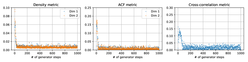
(a) SigCWGAN

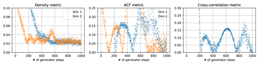
(b) CWGAN

Figure 1: Comparison across three performance metrics (see section 6) of training SigCWGAN with loss function (5) and CWGAN with loss function (2) for $2$-dimensional $\operatorname{VAR}(1)$, given by $X_{t+1}=\phi X_{t}+\epsilon_{t+1}$ with $(\epsilon_{t})_{t=1}^{T}$ iid Gaussian-distributed random variables with co-variance matrix $\sigma\mathbf{1}+(1-\sigma)\mathbf{I}$ and autocorrelation coefficient $\phi=0.8$ and co-variance parameter $\sigma=0.8$. The explicit form of the model allows for an unbiased approximation of conditional expectation in (2) using Monte Carlo samples. The colours blue and orange indicate the relevant distance/score for each dimension.

tting studied here, we lift both $(X_{\text{past}},X_{\text{future}})$ into the signature space, that is $(X_{\text{past}},X_{\text{future}})\mapsto(S_{\text{past}},S_{\text{future}}):=(S(X_{\text{past}}),S(X_{\text{future}}))$. The corresponding Sig-$W_{1}$ distance is given

$$\begin{split}\text{Sig-}W_{1}(\mu(S_{\text{past}}),\nu(S_{\text{past}}))&=\|\mathbb{E}_{S\sim\bm{\mu}(S_{\text{past}})}[S]-\mathbb{E}_{S\sim\bm{\nu}(S_{\text{past}})}[S]\|_{\mathrm{p}}\\ &=\|\mathbb{E}_{S\sim\bm{\mu}}[S_{\text{future}}\mid S_{\text{past}}]-\mathbb{E}_{S\sim\bm{\nu}}[S_{\text{future}}\mid S_{\text{past}}]\|_{\mathrm{p}}.\,.\end{split}$$

where $S$ denotes $(S_{\text{past}},S_{\text{future}})$. From Doob-Dynkin Lemma we know that the conditional expectations are measurable functions of $S_{\text{past}}$. Assuming the continuity of conditional expectation, and by the universal approximation results, these can be approximated arbitrarily well by linear functional of signature. Hence we have

$$\mathbb{E}_{S\sim\bm{\mu}}[|S_{\text{future}}-\mathbb{E}_{\bm{\mu}(S_{\text{past}})}[S_{\text{future}}]|^{2}]\approx\inf_{L\,\,\text{linear functional}}\mathbb{E}_{S\sim\bm{\mu}}[|S_{\text{future}}-L(S_{\text{past}})|^{2}]\,.$$ (4)

Due to linearity of the functional $L$, the solution of the above optimization problem can be estimated by linear regression.

Let $\hat{\bm{L}}$ denote the linear regression estimator of the conditional expectation $x\mapsto\mathbb{E}_{S\sim\bm{\mu}}[S_{\text{future}}|S_{\text{past}}=x]$.

Unlike classical $W_{1}$-GAN described above, the conditional expectation under the data measure needs to be computed only once. Complete training is then reduced to solving following supervised learning problem

$$\ell(\theta^{(g)}):=\mathbb{E}^{X_{\text{past}}}\left[||\hat{\bm{L}}(S_{\text{past}})-\mathbb{E}_{S_{\text{future}}\sim\bm{\nu}(\theta^{(g)},X_{\text{past}})}[S_{\text{future}}]||_{\mathrm{p}}\right]\,.$$ (5)

Note that for each $\theta^{(g)}$ one needs to approximate $\mathbb{E}_{S\sim\bm{\nu(\theta^{(g)})}}[S_{\text{future}}]$ using Monte Carlo simulations. A complete approximation algorithm also requires Monte Carlo approximation of outer expectation and truncation of the signature map (see Section 5.2 for exact details). The flowchart of SigCWGAN algorithm is given in Figure 2.

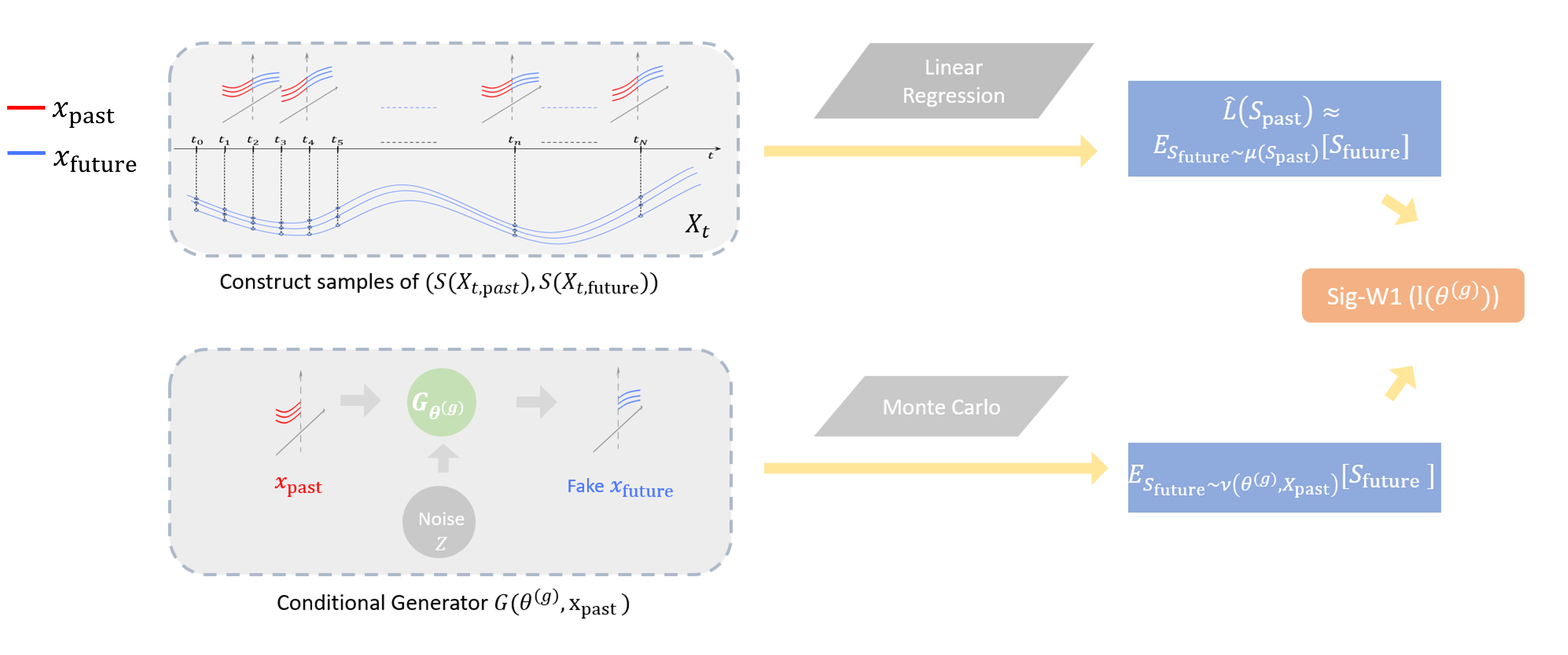
Figure 2: The illustration of the flowchart of SigCWGAN.

2.2 Related work

In the time series domain, the unconditional generative model was approached by various works such as Koshiyama et al. (2019); Wiese et al. (2020). Among the signature-based models, Kidger et al. (2019) used Sig-MMD, originated in Chevyrev and Oberhauser (2022), a version of the maximum mean discrepancy (MMD) with the signature feature, to generate the Ornstein–Uhlenbeck process. Independently, Ni et al. (2021) proposed the Sig-Wasserstein GAN motivated by combining the Wasssertain-1 distance and the signature feature. Also the conditional generative objective was approached by various authors. Esteban et al. (2017); Koochali et al. (2020); Fu et al. (2019); Wiese et al. (2019) used FNNs / LSTMs with recurrent conditional GANs (RCGANs), Donahue et al. (2019); Engel et al. (2019) use GANs to generating log-magnitude spectrograms and phases directly for audio synthesis, and Buehler et al. (2020) pair log-signatures with variational autoencoders (VAEs) and formulate a conditional generator in log-signature space. Conditional VAEs with the log-signature in Buehler et al. (2020) are well adapted to small data environment, but it may require an additional step of inverting synthetic log-signature to the path for time series generation. TimeGAN Yoon et al. (2019) demonstrates the improvement by adding the supervised loss to the adversarial loss to force network to adhere to the dynamics of the training data during sampling. The supervised loss of TimeGAN is defined in terms of the sample-wise discrepancy between the true latent variable $h_{t+1}$ and the generated one-sample estimator $\hat{h}_{t+1}$ given $h_{t}$. However, even if the estimator $\hat{h}_{t+1}$ has the same conditional distribution as $h_{t+1}$, the supervised loss may not be equal to zeros, and hence it suggests that the proposed loss function might not be suitable to capture the conditional distribution of the latent variable $h_{t+1}$ given the $h_{t}$.

Conditional moment matching network (CMMN) introduced in Ren et al. (2016) derives the conditional MMD criteria based on the kernel mean embedding of conditional distributions, which avoids the approximation issues mentioned in the above conditional WGANs. However, the performance of CMMN depends on the kernel choice and it is yet unclear how to choose the kernel on the path space. While our SigWGAN method is built on the conditional WGANs and the signature features, we would like to highlight the difference of method to the conditional WGAN and its link to CMMD. SigCWGAN resolves the computational bottleneck of the conditional WGANs given the past time series by using the analytic formula for the conditional discriminator without training. Building upon Ni et al. (2021), our work expands the SigWGAN framework from its initial application to unconditional generative models to enable conditional generative modelling. Moreover, one can view the SigCWGAN as the combination of unnormalized Sig-MMD (Chevyrev and Oberhauser (2022)) and CMMD, which has not been explored in the literature. It is worth noting that we also extend the definition of Sig-$W_{1}$ in Ni et al. (2021), from the $l^{2}$ norm of the signature space to the general $l^{\mathrm{p}}$ for some $\mathrm{p}>1$.

Symbol	meaning
$E$	$E=\mathbb{R}^{d}$
$T((E))$	the tensor algebra space of $E$
$\bf{T}^{\mathrm{p}}(E)$	the set of all the elements in $T((E))$ with finite $l^{\mathrm{p}}$ norm
$||.||_{\mathrm{p}}$	the $l^{\mathrm{p}}$ norm on $\mathbf{T}^{\mathrm{p}}(E)$
$||.||_{\mathrm{q}}$	the $l^{\mathrm{q}}$ norm on $T((E))^{*}$
$X$	$E$-valued time series of length $T$, i.e. $X=(X_{1},\cdots,X_{T})\in\mathbb{R}^{d\times T}$
$X_{t,\text{past}}$	the $\bar{p}$ lagged values of $X_{t}$, i.e. $(X_{t-p+1},\cdots,X_{t})\in\mathbb{R}^{d\times\bar{p}}=:\mathcal{X}$.
$X_{t,\text{future}}$	the next $\bar{q}$ step forecast of $X_{t}$, i.e. $(X_{t+1},\cdots,X_{t+\bar{q}})\in\mathbb{R}^{d\times\bar{q}}=:\mathcal{Y}$.
$\bar{p}$	the window size of the past path $X_{t,\text{past}}$
$\bar{q}$	the window size of the future path $X_{t,\text{future}}$
$S_{t,\text{past}}$	the signature of $X_{t,\text{past}}$
$S_{t,\text{future}}$	the signature of $X_{t,\text{future}}$

Table 1: Notation summary table

3 SIGNATURES and EXPECTED SIGNATURES

In order to introduce formally the optimal conditional time series discriminator, in this section we recall basic definitions and concepts from rough path theory.

3.1 Tensor algebra space

We start with introducing the tensor algebra space of $E$, where the signature of a $E$-valued path takes values. For simplicity, fix $E=\mathbb{R}^{d}$ throughout the rest of the paper. $E$ has the canonical basis $\left\{e_{1},\ldots,e_{d}\right\}$. Consider the successive tensor powers $E^{\otimes n}$ of $E$. If one thinks of the elements $e_{i}$ as letters, then $E^{\otimes n}$ is spanned by the words of length $n$ in the letters $\left\{e_{1},\ldots,e_{d}\right\}$, and can be identified with the space of real homogeneous non-commuting polynomials of degree $n$ in $d$ variables, i.e., $(e_{I}:=e_{i_{1}}\otimes\cdots\otimes e_{i_{n}})_{I=(i_{1},\cdots,i_{n})\in\{1,\cdots,d\}^{n}}$. We give the formal definition of the tensor algebra series as follows.

Definition 2

The space of all formal $E$-tensors series, denoted by $T\left(\left(E\right)\right)$ is defined to be the following space of infinite series:

$$T((E))=\left\{\mathbf{a}=(a_{0},a_{1},\cdots)\Big{|}a_{n}\in E^{\otimes n},\forall n\geq 0\right\}.$$

It is equipped with two operations, an addition and a product defined as follows: $\forall\mathbf{a}=(a_{0},a_{1},\cdots),\mathbf{b}=(b_{0},b_{1},\cdots)\in T((E))$, it holds that

$$\mathbf{a}+\mathbf{b} = (a_{0}+b_{0},a_{1}+b_{1},\cdots);$$

$$\mathbf{a}\otimes\mathbf{b} = (c_{0},c_{1},\cdots).$$

where $c_{n}=\sum_{j=0}^{n}a_{j}\otimes b_{n-j}$.

We endow the space $T((E))$ with the action of $\mathbb{R}$ by $\lambda\mathbf{a}=(\lambda a_{0},\lambda a_{1},\cdots)$ is a real non-communtative untial algebra with the unit $\mathbf{1}=(1,0,0,\cdots)$ Lyons et al. (2007).

Let us first introduce the function $||\cdot||_{\mathrm{p}}:T((E))\rightarrow[0,+\infty]$ for some $\mathrm{p}\geq 1$. For any element $\mathbf{a}:=\sum_{n\in\mathbb{N}}\sum_{I\in\{1,\cdots,d\}^{n}}a_{I}e_{I}\in T((E))$,

$$||a||_{\mathrm{p}}=\left(\sum_{n\in\mathbb{N}}|a_{n}|_{\mathrm{p}}^{\mathrm{p}}\right)^{1/\mathrm{p}},$$ (6)

where $|a_{n}|_{\mathrm{p}}=\left(\sum_{I\in\{1,\cdots,d\}^{n}}|a_{I}|^{\mathrm{p}}\right)^{\frac{1}{\mathrm{p}}}$.

Similarly, we define the map $||\cdot||_{\mathrm{q}}:T((E))^{*}\rightarrow[0,+\infty]$. Define the canonical basis of the dual space $T((E))^{*}$, i.e. $(e_{I}^{*})_{I=(i_{1},\cdots,i_{n})\in\{1,\cdots,d\}^{n},n\in\mathbb{N}}$ by $\langle e_{I_{1}}^{*},e_{I_{2}}\rangle=\mathbf{1}_{I_{1}=I_{2}}$. For any $L\in T((E))^{*}$, one can write

$$L=\sum_{n\in\mathbb{N}}\sum_{I\in\{1,\cdots,d\}^{n}}L_{I}e^{*}_{I}.$$

Then $||L||_{\mathrm{q}}$ is defined as

$$||L||_{\mathrm{q}}=\left(\sum_{n\in\mathbb{N}}\sum_{I=(i_{1},\cdots,i_{n})\in\{1,\cdots,d\}^{n}}|L_{I}|^{\mathrm{q}}\right)^{1/\mathrm{q}}.$$ (7)

In particular, we consider the subspace $\mathbf{T}^{\mathrm{p}}(E)$, consisting with all the elements $a\in T((E))$ with finite $||a||_{\mathrm{p}}$. In this case, $||\cdot||_{\mathrm{p}}$ becomes the $l^{\mathrm{p}}$ norm of $\mathbf{T}^{\mathrm{p}}((E))$.

Definition 3

Fix some $\mathrm{p}\geq 1$. We denote by $\mathbf{T}^{\mathrm{p}}(E)$ the following space equipped with the $l^{\mathrm{p}}$ topology:

$$\mathbf{T}^{\mathrm{p}}(E):=\left\{\mathbf{a}\in T((E))\big{|}\quad||\mathbf{a}||_{\mathrm{p}}<+\infty\right\}.$$

Furthermore, we define

$$\tilde{T}^{\mathrm{p}}(E)=\{\mathbf{a}\in\mathbf{T}^{\mathrm{p}}(E)\big{|}a_{0}=1\}.$$

In practice, instead of the signature (an infinite series of $E$-tensors), we often work with the truncated signature. Hence we introduce the corresponding truncated tensor algebra space.

Definition 4

Let $n\geq 1$ be an integer. Let $B_{n}=\{\mathbf{a}=(a_{0},a_{1},...)|a_{0}=...=a_{n}=0\}.$The truncated tensor algebra $T^{(n)}(E)$ of order $n$ over $E$ is defined as the quotient algebra

$$T^{(n)}(E)=T\left(\left(E\right)\right)/B_{n}.$$ (8)

The canonical homomorphism $T\left(\left(E\right)\right)\longrightarrow T^{(n)}(E)$ is denoted by $\pi_{n}$.

3.2 Signature of time series

Embed time series in the path space

The signature feature takes a continuous function perspective on discrete time series. It allows the unified treatment on irregular time series (e.g. variable length, missing data, uneven spacing, asynchronous multi-dimensional data) to the path space [Chevyrev and Kormilitzin (2016)]. To embed time series to the signature space, we first lift discrete time series to a continuous path of bounded $1$-variation.

Let $\bar{x}=(x_{t})_{t=1}^{T}\in\mathbb{R}^{\tilde{d}\times T}$ be a $\tilde{d}$-dimensional time series of length $T$. We embed $\bar{x}$ to $X:[0,T]\rightarrow\mathbb{R}^{d}$ with $d=\tilde{d}+1$ as follows: (1) Interpolate the cumulative sum process of $\bar{x}$ to get the $d$-dimensional piecewise linear path; (2) Add the time dimension to the $0^{th}$ coordinate of $X$.

Let $\Omega_{0}([0,T],\mathbb{R}^{d})$ denote the space of continuous $d$ dimensional paths of finite $1$-variation starting from the origin, with the $0^{th}$ coordinate being the time dimension. We endow $\Omega_{0}([0,T],\mathbb{R}^{d})$ with the $1$-variation metric. For any $\tilde{d}$-dimensional time series, its embedded path $X$ lives in $\Omega_{0}([0,T],\mathbb{R}^{d})$. Figure (3) gives one concrete example to illustrate the time series embedding.

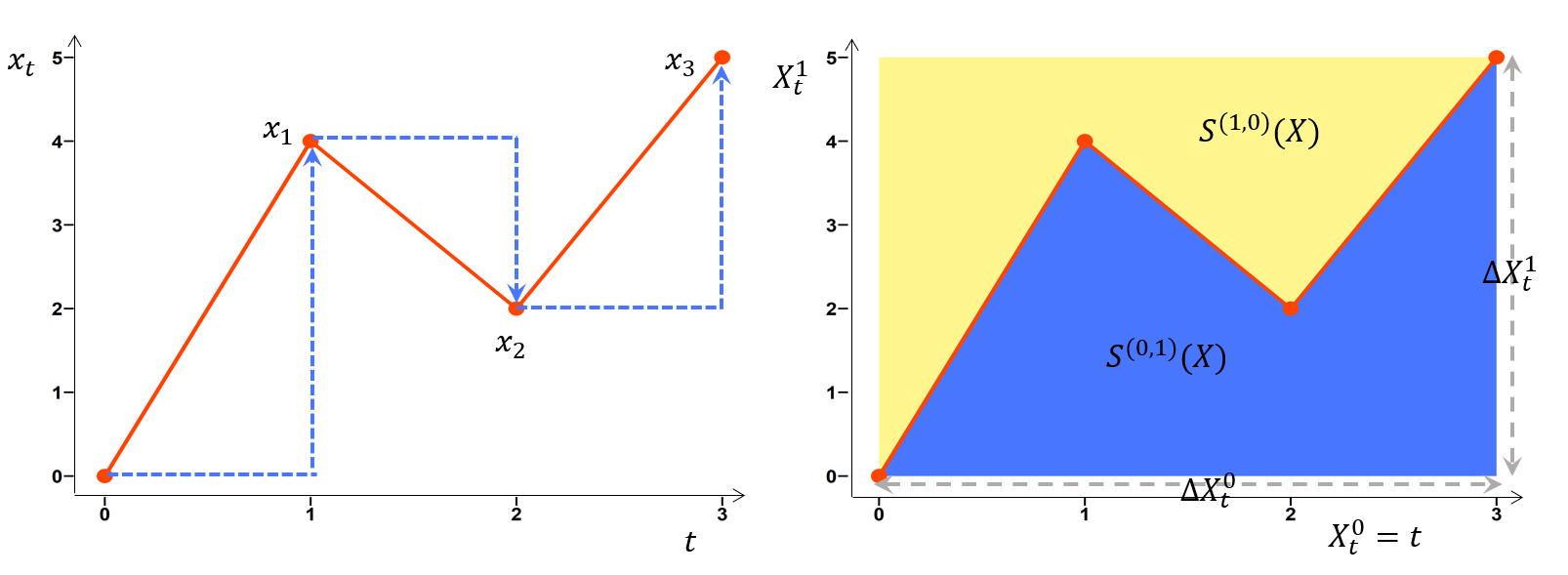
Figure 3: (Left) Embed one dimensional time series $\bar{x}=(x_{1},x_{2},x_{3})$ to $X$ (in blue) in the path space. First we compute $(X_{t})_{t=0}^{3}$, which is the cumulative sum of $(x_{t})_{t=1}^{3}$, i.e. $X_{0}=0$ and $X_{t}^{(1)}=\sum_{i=1}^{t}x_{i}$, $X_{t}^{(0)}=t$ for $t=1,2,3$. Then we linearly interpolate $X$ to a continuous path in $\Omega_{0}([0,3],\mathbb{R}^{2})$; (right) Embed the time series to the path space and visualize the low order signature.

Throughout the rest of the paper, we restrict our discussion on the path space $\Omega_{0}(J,E)$. However, our methodology discussed later can be applied to other methods of transforming discrete time series to the path space provided that the embedding ensures the uniqueness of the signature. The commonly-used path transformations with such uniqueness property are listed in Subsection B.1.

The signature of the path

We first introduce the $k$-fold iterated integral of a path $X\in\Omega_{0}([0,T],\mathbb{R}^{d})$. Let $I=(i_{1},\ldots,i_{k})$ be a multi-index of length $k$, where $i_{1},\ldots,i_{n}\in\{0,1,2,\cdots,d-1\}$. Let $X^{(i)}$ denote the $i^{th}$ coordinate of $X$, which is a real-valued function. The iterated integral of $x$ indexed by $I$ is defined as

$$S^{(i_{1},i_{2},\ldots,i_{k})}(X)=\int_{0<t_{1}<t_{2}<\cdots<t_{k}<T}dX_{t_{1}}^{(i_{1})}dX_{t_{2}}^{(i_{2})}\cdots dX_{t_{k}}^{(i_{k})}.$$

Collecting the iterated integrals of $X$ with all possible indices of length $k$ gives rise to the $k^{th}$ fold iterated integral of $X$. It can be also written in the tensor form, i.e.,

$$\int_{0\leq t_{1}\leq t_{2}\leq\cdots\leq t}dX_{t_{1}}\otimes dX_{t_{2}}\otimes\cdots\otimes dX_{t_{n}}\in E^{\otimes n}.$$

Figure 3 (Left) shows the $1$-fold iterated integral of $X$ which is the increment of $X$, i.e. $X_{3}-X_{0}$, and the $2$-fold iterated integral of $X$ which is given by

$$\mathbf{X}^{(2)}=(S^{(0,0)}(X),S^{(0,1)}(X),S^{(1,0)}(X),S^{(1,1)}(X)),$$

where $S^{(i,i)}(X)=\frac{1}{2}(\Delta X^{i})^{2}$ and $S^{(0,1)}(X),S^{(1,0)}(X)$ are blue and yellow area in Figure 3 (Right) respectively.

Now we are ready to introduce the signature of a path $X$.

Definition 5 (Signature of a path)

Let $X\in\Omega_{0}(J,E)$. The signature of the path $X$ is defined as

$$S(X)=(1,\mathbf{X}^{(1)},\mathbf{X}^{(2)},\ldots)\in T((E)),$$ (9)

where $\mathbf{X}^{(n)}=\int_{0\leq t_{1}\leq t_{2}\leq\cdots\leq t}dX_{t_{1}}\otimes dX_{t_{2}}\otimes\cdots\otimes dX_{t_{n}}$.

The truncated signature of the path $X$ of degree $M$, denoted by $S_{M}(X)$ and defined by

$$S_{M}(X):=\pi_{M}(S(X))=(1,\mathbf{X}^{(1)},\cdots,\mathbf{X}^{(M)}).$$

Lemma 6

Fix some $\mathrm{p}\geq 1$. For any $X\in\Omega_{0}([0,T],\mathbb{R}^{d})$, the signature of $X$ is an element of $\mathbf{T}^{\mathrm{p}}(E)$.

Proof  It is a consequence of the factorial decay of the signature of a path of bounded $1-$variation (c.f., Lemma 18 in Appendix A).  

Lemma 7 (Uniqueness of signature)

For any $X\in\Omega_{0}([0,T],E)$, the signature of $X$ uniquely determines $X$.

Proof  We refer the proof to that of Lemma 2.14 in Levin et al. (2013).  

The universality and uniqueness of signature, described in Section 2.1, make it an excellent candidate as a feature extractor of time series.

As we mainly work on the signature space in the later section, we provide a remark on the structure of the range of $S$ on $\Omega_{0}([0,T],E)$.

Remark 8

Let $\mathcal{K}$ denote a compact set of $\Omega_{0}([0,T],E)$. Then the range $S(\mathcal{K})$ is a compact set of $\mathbf{T}^{\mathrm{p}}(E)$ endowed with $l^{\mathrm{p}}$ topology. We defer the proof to that of Lemma 19 at Appendix A.

3.3 Expected signature

Expected signature

Since the signature $S$ is a bijective and continuous map when restricting the path space to $\Omega_{0}([0,T],E)$, the pushforward of the measure on the path space, $\bm{\mu}(B):=(S_{\#}\mu)(B)=\mu(S^{-1}(B))$ for $B$ in the $\sigma$-algebra of $S(\Omega_{0}([0,T],E))$, induces the measure on the signature space.

Lemma 9

Let $\mu,\nu$ be two measures defined on the path space $\Omega_{0}(J,E)$. Then for $\bm{\mu}(B):=(S_{\#}\mu)(B)$ and $\bm{\nu}(B):=(S_{\#}\nu)(B)$ with $B$ in the $\sigma$-algebra of $S(\Omega_{0}(J,E))$ we have

$$\bm{\mu}=\bm{\nu}\Longleftrightarrow\mu=\nu.$$

Proof  This is an immediate result of the bijective property of the signature map $S$, when $S$ is restricted to $\Omega_{0}(J,E)$.  

By Proposition 6.1 in Chevyrev et al. (2016), we have the following result:

Theorem 10

Let $\mu$ and $\nu$ be two measures on the path space $\Omega_{0}(J,E)$. Let $\bm{\mu}(B):=(S_{\#}\mu)(B)$ and $\bm{\nu}(B):=(S_{\#}\nu)(B)$ for $B$ is in the $\sigma$-algebra of $S(\Omega_{0}(J,E))$. Suppose that $\mathbb{E}_{S\sim\bm{\mu}}[S]$ exists and has infinite radius of convergence. If $\mathbb{E}_{S\sim\bm{\mu}}[S]=\mathbb{E}_{S\sim\bm{\nu}}[S]$, then $\mu=\nu$.

In other words, under the regularity condition, the distribution $\mu$ on the path space is characterized by $\mathbb{E}_{X\sim\mu}[S(X)]$. We call $\mathbb{E}_{X\sim\mu}[S(X)]$ the expected signature of the stochastic process $X$ under measure $\mu$. Intuitively, the signature of a path plays a role of a non-commutative polynomial on the path space. Therefore the expected signature of a random process can be viewed as an analogy of the moment generating function of a $d$-dimensional random variable. For example, the expected Stratonovich signature of Brownian motion determines the law of the Brownian motion in Lyons et al. (2015). However, it is challenging to establish a general condition to guarantee the infinite radius of convergence (ROC). In fact, the study of the expected signature of stochastic processes is an active area of research. For example, the expected signature of fractional Brownian motion for the Hurst parameter $H\geq 1/2$ is shown to have the infinite ROC Passeggeri (2020); Fawcett (2002), whereas the ROC of the expected signature of stopped Brownian motion up to the first exit domain is finite Boedihardjo et al. (2021); Li and Ni (2022). Theorem 6.3, Chevyrev et al. (2016) provides a sufficient condition for the infinite ROC of the expected signature, potentially offering an alternative way to show the infinite ROC without directly examining the decay rate of the expected signature.

4 SIG-WASSERSTEIN METRIC

In this section, we formalise the derivation of Signature Wasserstein-1 (Sig-$W_{1}$) metric introduced in Section 2.1. The Sig-$W_{1}$ is a generalisation of the one proposed in Ni et al. (2021) by considering the general $l^{\mathrm{p}}$ metric of the signature space.

Let $f:\Omega\rightarrow\mathbb{R}$, where $\Omega$ is a generic metric space. Define

$$||f||_{Lip,\Omega}:=\sup_{x\neq y,x,y\in\Omega}\frac{|f(x)-f(y)|}{D(x,y)},$$ (10)

where $D$ is a metric defined on $\Omega$. Let $\mu$ and $\nu$ be two compactly supported measures on the path space $\Omega_{0}([0,T],E)$ such that the corresponding induced measures on the signature space $\bm{\mu}$ and $\bm{\nu}$ respectively have a compact support $\mathcal{K}\subset S(\Omega_{0}([0,T],E))\subset\mathbf{T}^{\mathrm{p}}(E)$. Recall that

$$W_{1}^{\text{Sig}}(\mu,\nu) := W_{1}(\bm{\mu},\bm{\nu})=\sup_{||\bm{f}||_{Lip,\mathcal{K}}\leq 1}\mathbb{E}_{S\sim\bm{\mu}}[\bm{f}(S)]-\mathbb{E}_{S\sim\bm{\nu}}[\bm{f}(S)]\,.$$

From the definition of the supremum, there exists a sequence of $\bm{f}_{n}:\mathcal{K}\rightarrow\mathbb{R}$ with bounded Lipschitz norm along which the supremum $W^{\text{Sig}}_{1}(\mu,\nu)$ is attained. By the universality of the signature, it implies that for any $\epsilon>0$, for each $\bm{f}_{n}$, there exists a linear functional $\bm{L}_{n}:\mathcal{K}\rightarrow\mathbb{R}$ to approximate $\bm{f}_{n}$ uniformly, i.e.

$$|\int_{\mathcal{K}}\bm{f}_{n}(S)\bm{\mu}(dS)-\bm{f}_{n}(S)\bm{\nu}(dS)-\left(\int_{\mathcal{K}}\bm{L}_{n}(S)\bm{\mu}(dS)-\bm{L}_{n}(S)\bm{\nu}(dS))\right)|\leq 2\epsilon.$$

As $\bm{L}_{n}:\mathcal{K}\rightarrow\mathbb{R}$ is linear, there is a natural extension of $\bm{L}_{n}$ mapping from $\mathbf{T}^{\mathrm{p}}(E)$ to $\mathbb{R}$.

Motivated by the above observation, to approximate $W_{1}^{\text{Sig}}(\mu,\nu)$, we restrict the admissible set of $\bm{f}$ to be linear functionals $\bm{L}:T((E))\rightarrow\mathbb{R}$, which leads to the following definition:

Definition 11 ($\text{Sig-}W_{1}$ metric)

For two measures $\mu,\nu$ on the path space $\Omega_{0}([0,T],E))$ such that their induced measures $\bm{\mu}$ and $\bm{\nu}$ respectively has a compact support $\mathcal{K}\subset\mathcal{S}(\Omega_{0}([0,T],E))$,

$$\text{Sig-}W_{1}(\mu,\nu)=\sup_{||\bm{L}||_{Lip}\leq 1,L\text{ is a linear functional:}}\left(\mathbb{E}_{S\sim{\bm{\mu}}}[\bm{L}(S)]-\mathbb{E}_{S\sim\bm{\nu}}[\bm{L}(S)]\right).$$

Here we skip the domain $\mathbf{T}^{\mathrm{p}}(E)$ in the Lip norm of $||\mathbf{L}||_{Lip}$ for the simplicity of the notation.

Remark 12

Despite the motivation of $\text{Sig-}W_{1}$ from the approximation of $W^{Sig}_{1}$, it is hard to establish the theoretical results on the link between these two metrics. The main difficulty comes from that the uniform approximation of the continuous function $f$ by a linear map $L$ on $\mathcal{K}$ does not guarantee the closeness of their Lipschitz norms. We conjecture that in general $W_{1}^{Sig}(\mu,\nu)$ is not equal to $\text{Sig-}W_{1}(\mu,\nu)$. However, it would be interesting but technically challenging to find out the sufficient conditions such that these two metrics coincide.

To derive the analytic formulae for the Sig-$W_{1}$ metric, we shall introduce the following auxiliary lemma on the $l^{\mathrm{p}}$ norm of the tensor space $\mathbf{T}^{\mathrm{p}}(E)$ and its dual space.

Lemma 13

Fix $\mathrm{p},\mathrm{q}>1$ such that $\frac{1}{\mathrm{p}}+\frac{1}{\mathrm{q}}=1$ (i.e. $\mathrm{q}=\frac{\mathrm{p}}{\mathrm{p}-1}$).
For any linear functional $\bm{L}\in\mathbf{T}^{\mathrm{p}}(E)^{*}$, it holds that

$$\sup_{||a||_{\mathrm{p}}=1}|\bm{L}a|=||\bm{L}||_{\mathrm{q}},$$ (11)

Similarly, for any $a\in\mathbf{T}^{\mathrm{p}}(E)$, it holds that

$$\sup_{||\bm{L}||_{\mathrm{q}}\leq 1}|\bm{L}a|=\sup_{||\bm{L}||_{\mathrm{q}}=1}|\bm{L}a|=||a||_{\mathrm{p}}.$$ (12)

We refer to the proof of Lemma 13 in Appendix A.3.

Remark 14

The sequence space $L_{\mathrm{p}}(\mathcal{I})$ is defined as

$$L_{\mathrm{p}}(\mathcal{I})=\left\{(a_{I})_{I\in\mathcal{I}}\big{|}\sum_{I\in\mathcal{I}}|a_{I}|^{\mathrm{p}}<\infty\right\},$$

where $\mathcal{I}$ is a general index set and $\mathrm{p}\geq 1$. It is well known that the dual space of $L_{\mathrm{p}}(\mathcal{I})$ for $\mathrm{p}\geq 1$ has naturally isomorphic to $L_{\mathrm{q}}(\mathcal{I})$. This isomorphism is exactly the same as the map $L^{*}:\mathbf{T}^{\mathrm{p}}(E)\setminus\{0\}\rightarrow\mathbf{T}^{\mathrm{p}}(E)^{*}\setminus\{0\}:a\to L^{*}(a)$ used in our proof. Similarly, the dual space of $L_{\mathrm{p}}(\mathcal{I})^{*}$ has a natural isomorphism with $L_{\mathrm{p}}(\mathcal{I})$ for any $\mathrm{p}>1$.

By exploiting the linearity of the functional $\bm{L}\in\mathbf{T}^{\mathrm{p}}(E)^{*}$, we can compute the Lip norm of $L$ analytically for $D$ being the $l^{\mathrm{p}}$ norm of $\mathbf{T}^{\mathrm{p}}(E)$ without the need of numerical optimization. By Lemma 13, the Lip norm of $\bm{L}$ is the $L_{\mathrm{p}}$ norm of $\bm{L}$, given as

$$||\bm{L}||_{Lip}:=\sup_{x\neq y,x,y\in\mathbf{T}^{\mathrm{p}}(E)}\frac{|\bm{L}(x-y)|}{||x-y||_{\mathrm{p}}}=\sup_{||a||_{\mathrm{p}}=1}|\bm{L}a|=||\bm{L}||_{\mathrm{q}},$$

where $\frac{1}{\mathrm{p}}+\frac{1}{\mathrm{q}}=1$ and $D(x,y)=||x-y||_{\mathrm{p}}$ with some $\mathrm{p}>1$.

The simplification of the Lip norm enables us to derive an analytic formula of the corresponding Sig-$W_{1}$ metric.

Lemma 15

For two measures $\mu,\nu$ on the path space $\Omega_{0}([0,T],E)$ such that their induced measures $\bm{\mu}$ and $\bm{\nu}$ have a compact support $\mathcal{K}\subset S(\Omega_{0}([0,T],E))$. Then it holds that

$$\text{Sig-}W_{1}(\mu,\nu)=\|\mathbb{E}_{S\sim\bm{\mu}}[S]-\mathbb{E}_{S\sim\bm{\nu}}[S]\|_{\mathrm{p}}=\|\mathbb{E}_{X\sim\mu}[S(X)]-\mathbb{E}_{X\sim\nu}[S(X)]\|_{\mathrm{p}}.$$ (13)

Proof  Let a linear functional $\bm{L}:\mathcal{K}\rightarrow\mathbb{R}$ endowed with the Lip norm when $D(x,y)=||x-y||_{\mathrm{p}}$. In this case, the Lip norm coincides with $l^{\mathrm{q}}$ norm. The compact support $\mathcal{K}$ of $\bm{\mu}$ and $\bm{\nu}$ ensures that $\mathbb{E}_{S\sim\bm{\mu}}(S)$ and $\mathbb{E}_{S\sim\bm{\mu}}(S)$ are in $\mathbf{T}^{\mathrm{p}}(E)$. Let $a:=\mathbb{E}_{S\sim\bm{\mu}}(S)-\mathbb{E}_{S\sim\bm{\nu}}(X))$ and $a=(a_{I})_{I}$. Then by Lemma 13, one can derive the analytic formula of Sig-$W_{1}$ metric as follows:

$$\text{Sig-}W_{1}(\mu,\nu)=\sup_{||\bm{L}||_{\mathrm{q}}\leq 1}\bm{L}(\mathbb{E}_{S\sim\bm{\mu}}(S))-\bm{L}(\mathbb{E}_{S\sim\bm{\nu}}(S))=\sup_{||\bm{L}||_{\mathrm{q}}\leq 1}\bm{L}(a)=||a||_{\mathrm{p}}.$$

 

Remark 16

When $\mathrm{p}=2$, $\text{Sig-}W_{1}$ is the same as the unnormalised Sig-MMD metric proposed in Chevyrev and Oberhauser (2022). The theoretical results in Chevyrev and Oberhauser (2022) might be useful for studying the properties of Sig-Wasserstein metric.

Throughout the rest of the paper, by default, we use $\text{Sig-}W_{1}$ metric when $D$ is $l^{2}$ norm on $T((E))$, i.e. $\text{Sig-}W_{1}(\mu,\nu)=\|\mathbb{E}_{X\sim\mu}[S(X)]-\mathbb{E}_{X\sim\nu}[S(X)]\|_{2}$. In practice, we truncate the $\text{Sig-}W_{1}(\mu,\nu)$ up to degree $M$, i.e.

$$\text{Sig-}W_{1}^{M}(\mu,\nu)=\|\mathbb{E}_{X\sim\mu}[S_{M}(X)]-\mathbb{E}_{X\sim\nu}[S_{M}(X)]\|_{2}.$$

5 SIG-WASSERSTEIN GANS FOR CONDITIONAL LAW

In this section, we introduce a general framework, so-called Conditional Sig-Wasserstein GAN (SigCWGAN) based on Sig-$W_{1}$ metric to learn the conditional distribution $\mu(X_{\text{future}}|X_{\text{past}})$ from data $x$. The C-SigWGAN algorithm is mainly composed of two steps:

1. We apply a one-off linear regression to learn the conditional expected signature under true measure $\mathbb{E}_{X_{\text{future}}\sim\mu(X_{\text{past}})}[S(X_{\text{future}})]$ (see Section 5.1);

2. We solve an optimization problem to find optimal parameters $\theta^{(g)}$ of the conditional generator, when using loss (5) (see Section 5.2).

In the last subsection of this section, we propose a conditional generator, i.e. AR-FNN generator, which is a non-linear generalization of the classical autoregressive models by using a feed-forward neural network. It can generate the future time series of arbitrary length.

5.1 Learning the conditional expected signature under the true measure

The problem of estimating the conditional expected signature under the true measure $\bm{\mu}(S_{\text{past}})$, by Eqn. (4) and the universality of the signature (Theorem 1), can be viewed as a linear regression task, with the signature of the past path and future path respectively (Levin et al. (2013)).

More specifically, given a long realization of $x:=(x_{1},\cdots,x_{T})\in\mathbb{R}^{d\times T}$ and fixed window size of the past and future path $\bar{p},\bar{q}>0$, we construct the samples of past / future path pairs $(X_{\text{past}},X_{\text{future}})$ in a rolling window fashion, where the $i^{th}$ sample is given by

$$\left(x_{\text{past}}^{(i)},x_{\text{future}}^{(i)}\right)=(x_{\text{past},i+\bar{p}-1},x_{\text{future},i+\bar{q}-1}).$$

Assuming stationarity of the time series, the samples of past and future signature pairs are identically distributed

$$\left(S_{M_{1}}(x^{(i)}_{\text{past}}),S_{M_{2}}(x^{(i)}_{\text{future}})\right)_{i}\overset{d}{\sim}(S_{M_{1}}(X_{\text{past}}),S_{M_{2}}(X_{\text{future}})),$$

where $M_{1},M_{2}$ are the degrees of the signature of the past and future paths, which can be chosen by cross-validation in terms of fitting result. One may refer to Fermanian (2022) for further discussion on the choice of the degree of the signature truncation.

In principle, linear regression methods on the signature space could be applied to solve this problem using the above constructed data. When we further assume that under the true measure,

$$S_{M_{2}}(X^{(i)}_{\text{future}})=L(S_{M_{1}}(X^{(i)}_{\text{past}}))+\epsilon_{i},$$

where $\epsilon_{i}\overset{iid}{\sim}\epsilon$ and $\mathbb{E}[\epsilon_{i}|X^{(i)}]=0$, then an ordinary least squares regression (OLS) can be directly used. This simple linear regression model on the signature space achieves satisfactory results on the numerical examples of this paper. But it could be potentially replaced by other sophisticated regression models when dealing with other datasets.

We highlight that this supervised learning module to learn $\mathbb{E}_{\mu(X_{\text{past}})}[S_{M}(X_{\text{future}})]$ is one-off and can be done prior to the generative learning. It is in striking contrast to the conditional WGAN learning, which requires to learn $\mathbb{E}_{\mu(X_{\text{past}})}[f_{\alpha}(X_{\text{future}})]$ every time the discriminator $f_{\alpha}$ is updated, and hence saves significant computational cost.

5.2 Sig-Wasserstein GAN algorithm for conditional law

We recall that in order to quantify the goodness of the conditional generator $\nu(\theta^{(g)},x_{\text{past},t}):=G(\theta^{(g)},x_{\text{past}})_{\#}\mu_{z}$, we defined the loss

$$\ell(\theta^{(g)}):=\mathbb{E}^{X_{\text{past}}}\left[||\hat{\bm{L}}(S_{\text{past}})-\mathbb{E}_{S_{\text{future}}\sim\bm{\nu}(\theta^{(g)},X_{\text{past}})}[S_{\text{future}}]||_{\mathrm{p}}\right]\,,$$

where $\hat{\bm{L}}$ denotes the linear regression estimator for the conditional expectation $\hat{\bm{L}}:x\mapsto\mathbb{E}_{S\sim\bm{\mu}}[S_{\text{future}}|S_{\text{past}}=x]$. Given the conditional generator $G(\theta^{(g)},\cdot)$, the conditional expected signature $\mathbb{E}_{X\sim\nu(X_{\text{past}},\theta^{(g)})}[S(X)]$ can be estimated by Monte Carlo method. We denote by $\hat{\nu}_{i}$ the empirical approximation of $\nu(\theta,x_{\text{past}}^{(i)})$, computed by sampling the future trajectory $\hat{X}^{(t)}_{t+1:t+\bar{q}}$ using $G(\theta^{(g)},\cdot)$ and a conditioning variable $x_{\text{past},t}$. This leads to the following empirical loss function:

$$\ell^{(N)}(\theta^{(g)}):=\frac{1}{N}\sum_{i=1}^{N}||\hat{L}_{\mu}(S_{M_{1}}(x_{\text{past}}^{(i)})))-\mathbb{E}_{\hat{\nu}_{i}}[S_{M_{2}}(x_{\text{future}}^{(i)})]||_{\mathrm{p}}\,.$$ (14)

Using empirical loss function (14), one updates the generator parameters $\theta^{(g)}$ with stochastic gradient descent algorithm until it converges or achieves the maximum number of epochs. See Algorithm 1 for pseudocode.

Algorithm 1 Pseudocode of SigCWGAN

Input: $(x_{t})_{t=1}^{T}$, the signature degree of future path $M_{2}$, the signature degree of past path $M_{1}$, the length of future path $\bar{q}$, the length of past path $\bar{p}$, learning rate $\eta$, batch size $B$, the number of epochs $N$, number of Monte Carlo samples $N_{\text{MC}}$.
      Output: $\theta$ - the optimal parameter of the generator $G(\theta,\cdot)$.

1:Compute truncated signature of the past and future paths: $(S_{M_{1}}(x_{t-\bar{p}+1:t}),S_{M_{2}}(x_{t+1:t+\bar{q}}))_{t}$.

2:Compute linear regression coefficient $\hat{L}$ using $(S_{M_{1}}(x_{t-\bar{p}+1:t}),S_{M_{2}}(x_{t+1:t+\bar{q}}))_{t}$. (See Section 5.1.)

3:Initialise the parameters $\theta$ of the generator.

4:for $i=1:N$ do

5:     $\triangleright$ Denote the set of time index of the batch as $\mathcal{T}_{B}$.

6:     for $j=1:\#$ of batches do

7:         We randomly select the set of time index of batch size $B$, denoted by $\mathcal{T}$.

8:         Initialize $l^{(B)}(\theta)\leftarrow 0$.

9:         for $t\in\mathcal{T}_{B}$ do

10:              Simulate $n_{\text{MC}}$ samples of the simulated future path segments $(\hat{x}^{(j)})_{j=1}^{n_{\text{MC}}}$ by the generator $G(\theta,\cdot)$ given the past path $x_{t-\bar{p}+1:t}$.

11:              Compute

$$\hat{\mathbb{E}}_{X\sim\nu(\theta,x_{t-\bar{p}+1:t})}[S_{M_{2}}(X)]\leftarrow\frac{1}{n_{\text{MC}}}\sum_{j=1}^{n_{\text{MC}}}S_{M_{2}}(\hat{x}^{(j)}).$$

12:              Update $l^{(B)}(\theta)\leftarrow l^{(B)}(\theta)+\|\hat{L}(S_{M_{1}}(x_{t-\bar{p}+1:t}))-\hat{\mathbb{E}}_{X\sim\nu(\theta,x_{t-\bar{p}+1:t})}[S_{M_{2}}(X)]\|_{2}$.               

13:     $\theta\leftarrow\theta-\eta\frac{dl^{(B)}(\theta)}{d\theta}$. return $\theta$.

5.3 The Conditional AR-FNN Generator

In this subsection, we further assume that the target time series $X$ is stationary and satisfies the following autoregressive structure, i.e.

$$X_{t+1}=g(X_{t,\text{past}},\varepsilon_{t+1}),$$ (15)

where $f:\mathcal{X}\times\mathcal{Z}\rightarrow\mathbb{R}^{d}$ is continuous and $(\varepsilon_{t})_{t}$ are i.i.d. random variables and $\epsilon_{t}$ and $X_{t,\text{past}}$ are independent. Time series of such kind include the autoregressive model (AR) and the Autoregressive conditional heteroskedasticity (ARCH) model.

The proposed conditional AR-FNN generator is designed to capture the autoregressive structure of the target time series by using the past path $X_{\text{past},t}$ as additional input for the AR-FNN generator. The function $f$ in Eqn. (15) is represented by forward neural network with residual connections He et al. (2016) and parametric ReLUs as activation functions He et al. (2015) (see subsection B.2 for a detailed description).

We first consider a step-1 conditional generator $G_{1}(\theta^{(g)},\cdot):\mathbb{R}^{d\times\bar{p}}\times\mathcal{Z}\rightarrow\mathbb{R}^{d}$, which takes the past path $x$ and the noise vector $Z_{1}$ to generate a random variable to mimic the conditional distribution of step-1 forecast $\mu(X_{t+1}|X_{\text{past},t}=x)$. Here the noise vector $Z_{1}$ has the standard normal distribution in $\mathcal{Z}=\mathbb{R}^{d_{Z}}$.

One can generate the future time series of arbitrary length $\bar{q}\geq 1$ given $x_{\text{past}}$ by applying $G_{1}(\theta^{(g)},\cdot)$ in a rolling window fashion with i.i.d. noise vector $(Z_{t})_{t}$ as follows. Given $x_{\text{past}}=(\mathrm{x}_{1},\cdots,\mathrm{x}_{\bar{p}})\in\mathbb{R}^{d\times\bar{p}}$, we define time series $(\hat{x}_{t})_{t}$ inductively; we first initialize the first $\bar{p}$ term $\hat{x}$ as $x_{\text{past}}$, and then for $t>\bar{p}$, use $G_{1}(\theta^{(g)},\cdot)$ with the $\bar{p}$-lagged value of $\hat{x}_{t}$ conditioning variable and the noise $Z_{t}$ to generate $\hat{x}_{t+1}$; in formula,

$$\hat{x}_{t}=\begin{cases}\mathrm{x}_{t},&\text{ if }t\leq\bar{p};\\ G_{1}(\theta^{(g)},\underbrace{\hat{x}_{t-\bar{p}},\cdots,\hat{x}_{t-1}}_{\bar{p}\text{ lagged values of }\hat{x}_{t}},Z_{t}),&\text{ if }t>\bar{p}.\end{cases}$$ (16)

Therefore, we obtain the step-$\bar{q}$ conditional generator, denoted by $G_{q}(\theta^{(g)},\cdot):\mathbb{R}^{d\times\bar{p}}\rightarrow\mathbb{R}^{d\times\bar{q}}$ and defined by $x_{\text{past}}\mapsto\left(\hat{x}_{\bar{p}+1},\cdots,\hat{x}_{\bar{p}+\bar{q}}\right)$, where $\left(\hat{x}_{\bar{p}+1},\cdots,\hat{x}_{\bar{p}+\bar{q}}\right)$ is defined in Eqn. (16). We omit $\bar{q}$ in $G_{\bar{q}}$ for simplicity. (See Algorithm 2 in Supplementary Material.)

6 NUMERICAL EXPERIMENTS

To benchmark with SigCWGAN, we consider the baseline conditional WGAN (CWGAN) to compare the performance and training time. Besides, we benchmark SigCWGAN with three representative generative models for the time-series generation, i.e. (1) TimeGAN Yoon et al. (2019), (2) RCGAN Hyland et al. (2018) - a conditional GAN and (3) GMMN Li et al. (2015) - an unconditional maximum mean discrepancy (MMD) with Gaussian kernel. For a fair comparison, we use the same neural network generator architecture, namely the 3-layer AR-FNN described in subsection B.2, for all the above generative models. Furthermore, we compare the proposed SigCWGAN with Generalized autoregressive conditional heteroskedasticity model (GARCH), which is a popular econometric time series model.

To demonstrate the model’s ability to generate realistic multi-dimensional time series in a controlled environment, we consider synthetic data generated by the Vector Autoregressive (VAR) model, which is a key illustrative example in TimeGAN Yoon et al. (2019). We also provide two financial datasets, i.e. the SPX/DJI index data and Bitcoin-USD data to validate the efficacy of the proposed SigCWGAN model on empirical applications. The additional example of synthetic data generated by ARCH model is provided in the appendix.

To assess the goodness of the fitting of a generative model, we consider three main criteria (a) the marginal distribution of time series; (b) the temporal and feature dependence; (c) the usefulness Yoon et al. (2019) - synthetic data should be as useful as the real data when used for the same predictive purposes (i.e. train-on-synthetic, test-on-real). In the following, we give the precise definition of the test metrics. More specially, we use $\mathcal{D}_{\text{real}}:=(x_{\text{future}}^{(i)})_{i=1}^{N}$ and $\mathcal{D}_{\text{fake}}:=(\hat{x}_{\text{future}}^{(i)})_{i=1}^{N}$ to compute the test metrics, where $\hat{x}_{\text{future}}^{(i)}$ is a simulated future trajectory sampling by the conditional generator $G(\theta^{(g)},x^{(i)}_{\text{past}})$. $\mathcal{D}_{\text{real}}$ and $\mathcal{D}_{\text{fake}}$ are the samples of the $\mathbb{R}^{d\times\bar{q}}$-valued random variable $X_{\text{future}}$ under real measure and synthetic measure resp. The test metrics are defined below.

• Metric on marginal distribution: For each feature dimension $i\in\{1,\cdots,d\}$, we compute two empirical density functions (epdfs) based on the histograms of the real data and synthetic data resp. denoted by $\hat{df}_{r}^{i}$ and $\hat{df}_{G}^{i}$. We take the absolute difference of those two epdfs as the metric on marginal distribution averaged over feature dimension, i.e.,

  $$\frac{1}{d}\sum_{i=1}^{d}|\hat{df}_{r}^{i}-\hat{df}_{G}^{i}|_{1}.$$

• Metric on dependency:

  (1) Temporal dependency

  We use the absolute error of the auto-correlation estimator by real data and synthetic data as the metric to assess the temporal dependency. For each feature dimension $i\in\{1,\cdots,d\}$, we compute the auto-covariance of the $i^{th}$ coordinate of time series data $X$ with lag value $k$ under the real measure and the synthetic measure resp., denoted by $\rho_{r}^{i}(k)$ and $\rho_{G}^{i}(k)$. Then the estimator of the lag-1 auto-correlation of the real/synthetic data is given by $\frac{\rho_{r}^{i}(1)}{\rho_{r}^{i}(0)}$/ $\frac{\rho_{G}^{i}(1)}{\rho_{G}^{i}(0)}$. The ACF score is defined to be the absolute difference of lag-1 auto-correlation given as follows:

  $$\frac{1}{d}\sum_{i=1}^{d}\left|\frac{\rho_{r}^{i}(1)}{\rho_{r}^{i}(0)}-\frac{\rho_{G}^{i}(1)}{\rho_{G}^{i}(0)}\right|.$$

  Note $\rho_{r}^{i}(k)$ and $\rho_{r}^{i}(k)$ can be estimated empirically by Eqn. (21) and Eqn. (22) in Appendix C resp, which allows us to compute the ACF score on the dataset. In addition, we present the ACF plot, which illustrates the autocorrelation of each coordinate of the time series with different lag values. The synthetic data’s quality is evaluated by how closely its ACF plot resembles that of the real data, as it indicates the synthetic data’s ability to capture long-term temporal dependencies.

  (2) Feature dependency

  For $d>1$, we use the $l^{1}$ norm of the difference between cross correlation matrices. Let $\tau^{i,j}_{r}$ and $\tau^{i,j}_{G}$ denote the correlation of the $i^{th}$ and $j^{th}$ feature of time series under real measure and synthetic measure resp. The metric on the correlation between the real data and synthetic data is given by $l^{1}$ norm of the difference of two correlation matrices, i.e.

  $$\sum_{i=1}^{d}\sum_{j=1}^{d}|\tau^{i,j}_{r}-\tau^{i,j}_{G}|.$$

  We defer the estimation of the correlation matrix $\tau^{i,j}_{r}$ and $\tau^{i,j}_{G}$ from the true data and fake data to Appendix C.

• $R^{2}$ comparison: Following Esteban et al. (2017) and Yoon et al. (2019), we consider the problem of predicting next-step temporal vectors using the lagged values of time series using the real data and synthetic data. First, we train a supervised learning model on real data and evaluate it in terms of $R^{2}$(TRTR). Then we train the same supervised learning model on synthetic data and evaluate it on the real data in terms of $R^{2}$ (TSTR). The closer two $R^{2}$ are, the better the generative model it is. To assess the performance of the proposed SigCWGAN to generate the longer time series, we consider the $R^{2}$ score for the regression task to predict the next $q$-step, where $q$ can be even larger than $\bar{q}$.

The train and test split is 80% and 20% respectively in all the numerical examples. We conduct the hyper-parameter tuning for the signature truncation level. We set $\mathrm{p}=2$ in the $l^{\mathrm{p}}$ norm used in the $\text{Sig-}W_{1}$ metric. Appendix B contains the additional information on implementation details of SigCWGAN, including path transformations and network architecture of the generator. We refer the Appendix C for more details on the evaluation metrics. We also provide the extensive supplementary numerical results of $\operatorname{VAR}(1)$ data, $\operatorname{ARCH}(1)$ data and empirical data in Appendix D. Implementation of SigCWGAN can be found in https://github.com/SigCGANs/Conditional-Sig-Wasserstein-GANs.

6.1 Synthetic data generated by Vector Autoregressive Model

In the $d$-dimensional $\operatorname{VAR}(1)$ model, time series $(X_{t})_{t=1}^{T}$ are defined recursively for $t\in\{1,\dots,T-1\}$ through

$$X_{t+1}=\phi X_{t}+\epsilon_{t+1},$$ (17)

where $(\epsilon_{t})_{t=1}^{T}$ are iid Gaussian-distributed random variables with co-variance matrix $\sigma\mathbf{1}+(1-\sigma)\mathbf{I}$; $\mathbf{I}$ is a $d\times d$ identity matrix. Here, the coefficient $\phi\in[-1,1]$ controls the auto-correlation of the time series and $\sigma\in[0,1]$ the correlation of the $d$ features. In our benchmark, we investigate the dimensions $d=1,2,3$ and various $(\sigma,\phi)$. We set $T=40000$ and $\bar{p}=\bar{q}=3$. In this example, the optimal degree of signature of both past paths and future paths is 2.

First, we empirically prove that the proposed SigCWGAN can serve as an enhancement of CGWAN model. One can see from Figure 4, when the CWGAN training is fed into a more reliable estimator of the conditional mean under real measure $\mathbb{E}_{\mu(x_{\text{past}})}[f(X_{\text{future}})]$, the training tends to converge faster. However, the commonly-used one-sample estimator ($x_{\text{future}}$) in the CWGAN training may suffer from large variance, leading to inefficiency of training. In contrast to it, the SigCWGAN may alleviate this problem by its supervised learning module. Additionally, the simplification of the min-max game to optimization via SigCWGAN leads to further acceleration and stabliziation of training SigCWGANs, and hence brings the performance boost, as shown in Table 2. Figure 4 illustrates that the SigCWGAN has a better fitting than CWGAN in terms of conditional law as the estimated mean (and standard deviation) is closer to that of the true model compared with CWGAN. Moreover, Table D.1- D.3 show that the SigCWGAN consistently beats the CWGAN in terms of performance for varying $d$, $\phi$ and $\sigma$.

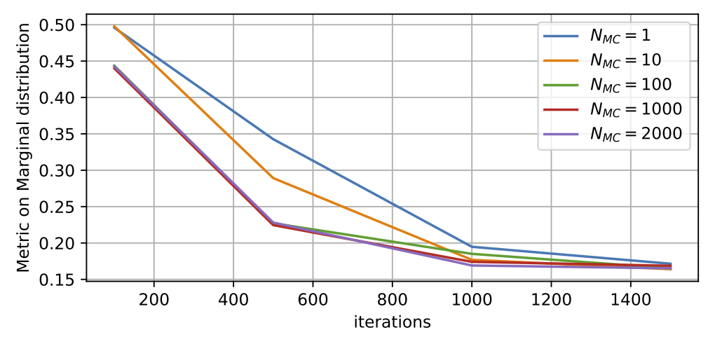
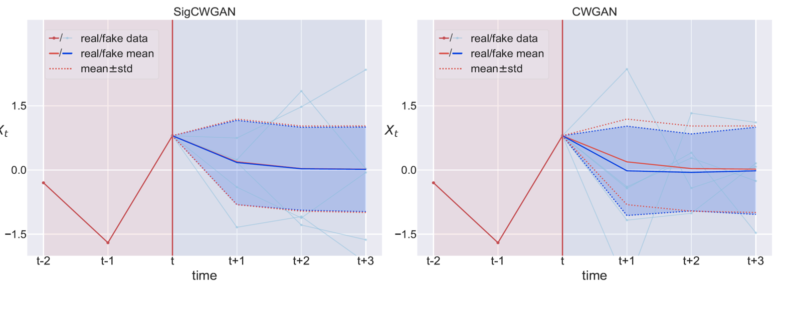
Figure 4: (Left) Comparison of the performance on CWGAN in terms of metric on the marginal distribution for varying $N_{\text{MC}}$. This experiment is conducted on a 3-dimensional VAR(1) dataset generated by Eqn.(17) with $\phi=\sigma=0.8$. We use the Monte-Carlo estimator of the conditional mean ($\mathbb{E}_{\mu(x_{\text{past}})}[f(\theta^{(d)})(X_{\text{future}})]$) generated by the ground truth model for the CWGAN training. The larger number $N_{\text{MC}}$ of Monte Carlo approximation, the better conditional mean under the true measure. (Right) Comparison of the performance of SigCWGAN and CWGAN in terms of fitting the conditional distribution of future time series given one past path sample on 1-dimensional VAR(1) dataset.

Metrics	marginal distribution	auto-correlation	$R^{2}(\%)$	Sig-$W_{1}$
SigCWGAN	0.0314	0.0085	0.0394	0.4286
CWGAN	0.0086	0.0110	0.0350	0.4384
TimeGAN	0.0243	0.0320	0.0229	0.4680
RCGAN	0.0095	0.0332	0.0214	0.4466
GMMN	0.0084	0.0298	0.0026	0.4499

Table 2: Numerical results of $\operatorname{VAR}(1)$ for $d=3$ with fixed training time of 2 minutes

We then proceed with the comparison of CSigWGN with the other state-of-the-art baseline models. Across all dimensions, we observe that the CSigWGAN has a comparable performance or outperforms the baseline models in terms of the metrics defined above. In particular, we find that as the dimension increases the performance of SigCWGANs exceeds baselines. We illustrate this finding in Figure 5 which shows the relative error of TSTR $R^{2}$ when varying the dimensionality of $\operatorname{VAR}(1)$. Observe that the SigCWGAN remains a very low relative error, but the performance of the other models deteriorates significantly, especially the GMMN.

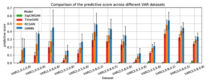
Figure 5: Comparison of predictive score across the VAR(1) datasets. The three numbers in the bracket indicate the hyperparameters $d,\phi,\sigma$ used to generate the corresponding VAR dataset. The predictive score was computed by taking the absolute difference of the $R^{2}$ obtained from TSTR and TRTR.

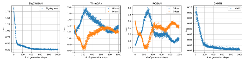
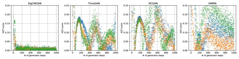
Figure 6: (Upper panel) Evolution of the training loss functions. (Lower panel) Evolution of the ACF scores. Each colour represents the ACF score of each feature dimension. Results are for the 3-dimensional $\operatorname{VAR}(1)$ model based on Eqn. (17) for $\phi=0.8$ and $\sigma=0.8$.

Moreover, we validate the training stability of different methods. Figure 6 shows the development of the loss function and ACF scores through the course of training for the 3-dimensional $\operatorname{VAR}(1)$ model. It indicates the stability of the SigCWGAN optimisation in terms of training iterations, in contrast to all the other algorithms, especially RCGAN and TimeGAN that involve a min-max optimisation, as identified in the 1st Challenge in Section 2. While the ACF scores of the baseline models oscillate heavily, the SigCWGAN ACF score and Sig-$W_{1}$ distance converge nicely towards zero. Also, although the MMD loss converges nicely towards zero, in contrast, the ACF scores do not converge. This highlights the stability and usefulness of the Sig-$W_{1}$ distance as a loss function.

To assess the efficiency of different algorithms, we train all the algorithms for the same amount of time (2 minutes) and compare the test metrics of each method. Table 2 show a higher efficiency of SigCWGAN, which yields the best performance in terms of all the metrics except for the metric on the marginal distribution.

Furthermore, the SigCWGAN has the advantage of generating the realistic long time series over the other models, which is reflected by that the marginal density function of a synthetic sampled path of 80,000 steps is much closer to that of real data than baselines in Figure 7.

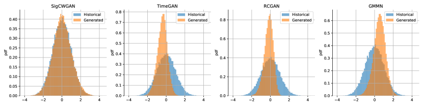
Figure 7: Comparison of the marginal distributions of one long sampled path (80,000 steps) with the real distribution.

6.2 SPX and DJI index dataset

The dataset of the S$\&$P 500 index (SPX) and Dow Jones index (DJI) consists time series of indices and their realized volatility, which is retrieved from the Oxford-Man Institute’s ”realised library”Heber et al. (2009). We aim to generate a time series of both the log return of the close prices and the log of median realised volatility of (a) the SPX only; (b) the SPX and DJI. Here we choose the length of past and future path to be $3$. By cross-validation, the optimal degree of signature ($M_{1}=M_{2}$) is 3 and 2 for the SPX dataset and SPX/DJI dataset, respectively.

Table 3 shows that SigCWGAN achieves the superior or comparable performance to the other baselines. The SigCWGAN generates the realistic synthetic data of the SPX and DJI data shown by the marginal distribution comparison with that of real data in Figure 8. For the SPX only data, GMMN performs slightly better than our model in terms of the fitting of lag-1 auto-correlation and marginal distribution ($\leq 0.0013$), but it suffers from the poor predictive performance and feature correlation in Table 3 and Figure 9. When the SigCWGAN is outperformed, the difference is negligible. Furthermore, the test metrics, i.e. the ACF loss and density metric, of our model are evolving much smoother than the test metrics of the other baseline models shown in Figure D.7. Moreover, the ACF plot shown in Figure 9 shows that SigCWGAN has the better fitting for the auto-correlation for various lag values, which indicates the superior performance in terms of capturing long temporal dependency.

It is worth noting that our SigCWGAN model outperforms GARCH, the classical and widely used time series model in econometrics, on both the SPX and SPX/DJI data, as shown in Table 3. The poor performance of the GARCH model could be attributed to its parametric nature and the potential issues of model mis-specification when applied to empirical data.

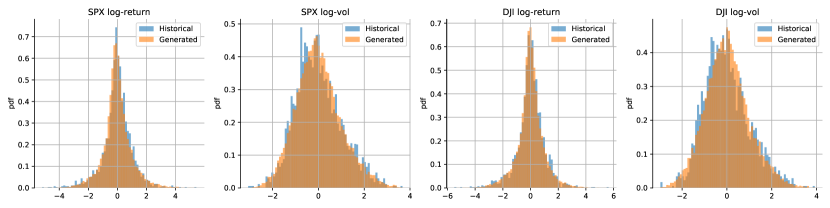
Figure 8: Comparison of the marginal distributions of the generated SigCWGAN paths and the SPX and DJI data.

Metrics	marginal distribution	auto-correlation	correlation	$R^{2}(\%)$	Sig-$W_{1}$
SigCWGAN	0.01730, 0.01674	0.01342, 0.01192	0.01079, 0.07435	2.996, 7.948	0.18448, 4.36744
TimeGAN	0.02155, 0.02127	0.05792, 0.03035	0.12363, 0.61488	5.955, 8.586	0.58541, 5.99482
RCGAN	0.02094, 0.01655	0.03362, 0.04075	0.04606, 0.15353	2.788, 7.190	0.47107, 5.43254
GMMN	0.01608, 0.02387	0,01283, 0.02676	0.04651, 0.22380	9.049, 7.384	0.59073, 6.23777
GARCH	0.01583,0.01670	0.13392, 0.11337	0.15791, 0.7290	12.1253, 12.5686	0.64825, 6.15344

Table 3: Numerical results of the stock datasets. In each cell, the left/right number are the result for the SPX data/ the SPX and DJI data respectively. We use the relative error of TSTR $R^{2}$ against TRTR $R^{2}$ as the $R^{2}$ metric.

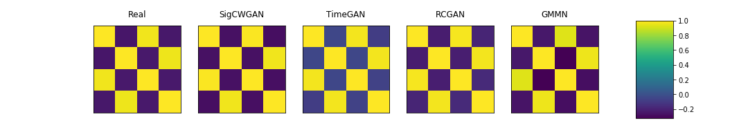
Figure 9: Comparison of real and synthetic cross-correlation matrices for SPX and DJI log-return and log-volatility data. On the far left the real cross-correlation matrix from SPX and DJI data is shown. $x$/$y$-axis represents the feature dimension while the color of the $(i,j)^{th}$ block represents the correlation of $X_{t}^{(i)}$ and $X_{t}^{(j)}$. The color bar on the far right indicates the range of values taken.

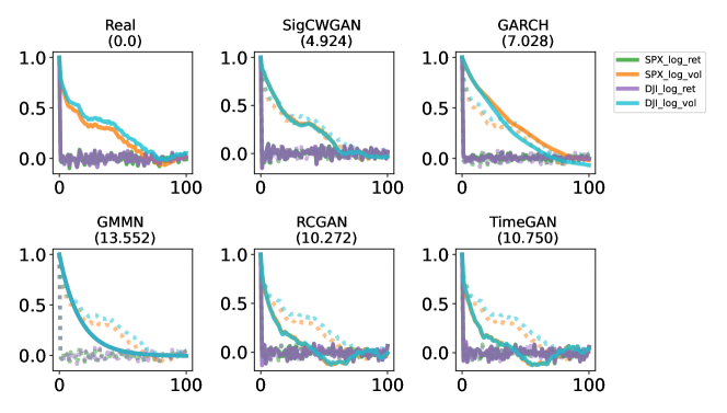
Figure 10: ACF plot for each channel on the SPX/DJI dataset. Here x-axis represents the lag value ( with maximum lag equal to 100) and y-axis represent the corresponding auto-correlation. The length of real/generated time series used to compute the ACF is 1000. The number in the bracket under each model is the sum of the absolute difference between the correlation coefficients computed from real (dashed line) and generated (solid line) samples.

6.3 Bitcoin-USD dataset

The Bitcoin-USD dataset contains hourly data of Bitcoin price in USD from 2021 to 2022. We use the data in 2021 (2022) for the training (testing), respectively, which are illustrated in Figure 11. We apply our method to learn the future log-return of the future 6 hours given the past 24 hours. We encode the future and past paths with their signatures of depth 4. Table 4 demonstrates that our proposed SigCWGAN outperforms the other baselines in terms of almost all the test metrics. The $R^{2}$ score of the RCGAN (0.3165) is slightly better than that of the SigCWGAN by 0.0155, whilst SigCWGAN achieves superior performance than the RCGAN in terms of other metrics, especially marginal distribution (2.0532 v.s. 2.803). The better performance of the SigCWGAN to capture the temporal dependency is also verified by the additional results of the autocorrelation metric and the $R^{2}$-metric for different lag values are provided in tables D.8 and D.9.

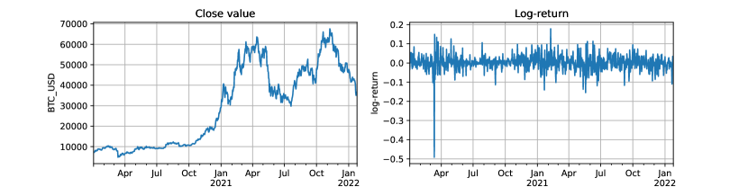
Figure 11: The evolution of the close value (Left) and log return of BTC-USD from January 2021 to January 2023.

Metrics	marginal distribution	auto-correlation	$R^{2}(\%)$	Sig-$W_{1}$
SigCWGAN	2.0532	0.091	0.3320	0.0829
TimeGAN	2.8037	0.1203	0.7582	0.1675
RCGAN	2.8603	0.0532	0.3165	0.0994
GMMN	2.8212	0.2093	0.3904	0.0846
GARCH	4.5063	0.0872	123.77	2.73

Table 4: Numerical results of BTC-USD data experiment. We use the relative error of TSTR $R^{2}$ against TRTR $R^{2}$ as the $R^{2}$ metric.

7 Conclusion

In this paper, we developed the conditional Sig-Wasserstein GAN for time series generation based on the explicit approximation of $W_{1}$ metric using the signature features space. This eliminates the problem of having to approximate a costly critic / discriminator and, as a consequence, dramatically simplifies training. Our method achieves state-of-the-art results on both synthetic and empirical dataset.

Our proposed conditional Sig-Wasserstein GAN is proved to be effective for generating time series of a moderate dimension. However, it may suffer the curse of dimensionality caused by high path dimension. It might be interesting to explore how to combine SigCWGAN with the implicit generative model to learn the low dimensional latent embedding and hence cope with the high dimensional path case. Moreover, on the theoretical level, it is worthy of investigating the conditions, under which the $W_{1}$ metric on the signature space coincides with the Sig-$W_{1}$ metric.

Acknowledgments

HN is supported by the EPSRC under the program grant EP/S026347/1. HN and LS are supported by the Alan Turing Institute under the EPSRC grant EP/N510129/1. All authors thank the anonymous referees for constructive feedback, which greatly improves the paper. Moreover, HN extends her gratitude to Siran Li, Terry Lyons, Chong Lou, Jiajie Tao, and Hang Lou for their helpful discussion.

Data Availability Statement

The data that support the findings of this study are openly available in Conditional-Sig-Wasserstein-GANs repository at https://github.com/SigCGANs/Conditional-Sig-Wasserstein-GANs. These empirical data were derived from the following resources available in the public domain: (1) the Oxford-Man Institute’s ”realised library” https://realized.oxford-man.ox.ac.uk/data;(2) https://github.com/David-Woroniuk/Historic_Crypto.

A PRELIMINARY

For the sake of precision, we start by introducing basic concepts around the signature of a path, which lays the foundation for our analysis on the signature approximation for Wasserstein-1 Distance. We complete this section by providing the proof of Lemma 13, which is essential for the derivation of the proposed Sig-W₁ metric.

A.1 Signature of a path

We introduce the $p$-variation as a measure of the roughness of the path. For ease of notation, let $J$ denote a compact time interval.

Definition 17 ($p$-Variation)

Let $p\geq 1$ be a real number. Let $X:J\rightarrow E$ be a continuous path. The $p$-variation of $X$ on the interval $J$ is defined by

$$||X||_{p,J}=\left[\sup_{\mathcal{D}\subset J}\sum_{j=0}^{r-1}\left|X_{t_{j+1}}-X_{t_{j}}\right|^{p}\right]^{\frac{1}{p}},$$ (18)

where the supremum is taken over any time partition of $J$, i.e. $\mathcal{D}=(t_{1},t_{2},\cdots,t_{r})$.

Let $\mathcal{C}^{p}(J,E)$ denote the set of all continuous paths mapping from $J$ to $E$ of finite $p$-variation. The larger the $p$-variation is, the rougher a path is. The compactness of the time interval $J$ cannot ensure the finite $1$-variation of a continuous path in general. For example, Brownian motion has $(2+\varepsilon)$-variation a.s $\forall\varepsilon>0$, but it has infinite $p$-variation a.s.$\forall p\in[1,2]$.

For each $p\geq 1$, the $p$-variation norm of a path $X\in\mathcal{C}_{p}(J,E)$ is denoted by $||X||_{p-var}$ and defined as follows:

$$||X||_{p-var}=||X||_{p,J}+\sup_{t\in J}||X_{t}||.$$

Recall that $\pi_{n}$ is the projection map from the tensor algebra element to its truncation up to level $n$. To differentiate with $\pi_{n}$, we also introduce another projection map $\Pi_{n}:T((E))\rightarrow E^{\otimes n}$, which maps any $\mathbf{a}=(a_{0},a_{1},\cdots,a_{n},\cdots)$ to its $n^{th}$ term $a_{n}$.

For concreteness, we state the decay rate of the signature for paths of finite $1$-variation. However, there is a similar statement of the factorial decay for the case of paths of finite $p$-variation Lyons et al. (2007).

Lemma 18 (Factorial Decay of the Signature)

Let $X\in\mathcal{C}_{1}(J,E)$. Then there exists a constant $C>0$, such that for all $m\geq 0$,

$$|\Pi_{m}(S(X))|\leq C\frac{|X|_{1-var}^{m}}{m!}.$$

Lemma 19

Let $\mathcal{K}$ denote a compact set of $\Omega_{0}([0,T],E)$. Then the range $S(\Omega_{0}([0,T],E))$ is a compact set on $T^{\mathrm{p}}(E)$ endowed with $l^{\mathrm{p}}$ topology.

Proof  The proof boils down to showing the continuity of the signature map $S$ from $\Omega_{0}([0,T],E)$ with $1-$variation norm to $\mathbf{T}^{\mathrm{p}}(E)$ with $l^{\mathrm{p}}$ topology. Let $X,Y\in\Omega_{0}([0,T],E)$, which are controlled by the control function $\omega$, e.g., $\omega(s,t):=\max(|X_{s,t}|_{1-var},|Y_{s,t}|_{1-var})$ for all $0<s<t<T$. Let $|X_{[s,t]}-Y_{[s,t]}|_{1-var}\leq\epsilon\omega(s,t)$ for some $\epsilon\in\mathbb{R}^{+}$. Then by the continuity of the signature map in Theorem 3.10, Lyons et al. (2007) and the admissible norm $l^{1}$, it holds that for an integer $n\geq 1$,

$$|\Pi_{m}(S(X))-\Pi_{m}(S(Y))|_{1}\leq\epsilon\frac{\omega(0,T)^{m}}{\beta n!},$$

where $\beta=2\left(1+\sum_{r=3}^{\infty}\left(\frac{2}{r-2}\right)^{2}\right)$. The direct calculation leads to that

$$||S(X)-S(Y)||_{\mathrm{p}}\leq||S(X)-S(Y)||_{\mathrm{1}}\leq\sum_{m=1}^{\infty}\left(\epsilon\frac{\omega(0,T)^{m}}{\beta m!}\right)=\frac{\epsilon}{\beta}\sum_{m=1}^{\infty}\left(\frac{\omega(0,T)^{m}}{m!}\right)<+\infty.$$

 

A.2 Expected Signature of stochastic processes

Definition 20

Let $X$ denote a stochastic process, whose signature is well defined almost surely. Assume that $\mathbb{E}[S(X)]$ is well defined and finite. We say that $\mathbb{E}[S(X)]$ has infinite radius of convergence, if and only if for every $\lambda\geq 0$,

$$\sum_{n\geq 0}\lambda^{n}|\Pi_{n}(\mathbb{E}[S(X)])|<\infty.$$

A.3 The Signature Wasserstein-1 metric (Sig-$W_{1}$)

In the following, we provide the proof of Lemma 13.

Proof  Let $\left(e_{I}=e_{i_{1}}\otimes\cdots e_{i_{n}}\right)_{I}$ be the canonical basis of $T((E))$. For any $a\in T((E))$, we write $a=(a_{I})$, i.e. $a=\sum_{I}a_{I}e_{I}$. Then $\left(e_{I}^{*}=e^{*}_{i_{1}}\otimes\cdots e^{*}_{i_{n}}\right)_{I=(i_{1},\cdots,i_{n})}$ is the basis of $T((E))^{*}$ and we can write $L=\sum_{I}l_{I}e^{*}_{I}$.

To prove Eq. (11), we solve the constraint optimization of maximising $\bm{L}a$ with the constraint $||a||_{p}=1$ by the Lagrange multiplier method. W.l.o.g, we only prove the case for $L\neq 0$ as it is trivial for $\bm{L}=0$, (when $L=0$, $La\equiv 0$, $||\bm{L}||_{q}=0$, and Eq. (11) holds). More specifically, we solve the unconstrained optimisation

$$\mathcal{L}(a,\lambda):=\sup_{a}|\bm{L}a|+\lambda\left(\sum_{I}|a_{I}|^{\mathrm{p}}-1\right),$$

where $\bm{L}\neq 0$.
The optimal $(a^{*},\lambda^{*})$ is a solution to the below equations:

$$\frac{\partial{\mathcal{L}}}{\partial a_{I}}=(\text{sign}(a_{I}l_{I})l_{I}+(\lambda(\mathrm{p}|a_{I}|^{\mathrm{p}-1}\text{sign}(a_{I}))))=0,\forall I$$

$$\frac{\partial{\mathcal{L}}}{\partial\lambda}=\sum_{I}|a_{I}|^{\mathrm{p}}-1=0.$$

Then we obtain that $a^{*}=(a_{I}^{*})_{I}$ with $a^{*}_{I}=\text{sign}(l_{I})\frac{|l_{I}|^{\frac{1}{\mathrm{p}-1}}}{(\sum_{I}|l_{I}|^{\mathrm{p}/(\mathrm{p}-1)})^{1/\mathrm{p}}}=\text{sign}(l_{I})\frac{|l_{I}|^{\frac{1}{\mathrm{p}-1}}}{(\sum_{I}|l_{I}|^{\mathrm{q}})^{1/\mathrm{p}}}$. Then it follows that

$$l_{I}a^{*}_{I}=|l_{I}|\cdot\frac{|l_{I}|^{\frac{1}{\mathrm{p}-1}}}{(\sum_{I}|l_{I}|^{\mathrm{q}})^{1/\mathrm{p}}}=\frac{|l_{I}|^{\mathrm{q}}}{(\sum_{I}|l_{I}|^{\mathrm{q}})^{1/\mathrm{p}}}\geq 0;$$

$$|La^{*}|=La^{*}=\sum_{I}l_{I}a^{*}_{I}=\frac{\sum_{I}|l_{I}|^{\mathrm{q}}}{\left(\sum_{I}|l_{I}|^{\mathrm{q}}\right)^{1/\mathrm{p}}}=(\sum_{I}|l_{I}|^{\mathrm{q}})^{1-1/\mathrm{p}}=(\sum_{I}|l_{I}|^{\mathrm{q}})^{1/\mathrm{q}}=||L||_{\mathrm{q}}.$$

By Hôlder’s inequality,

$$\sup_{||a||_{\mathrm{p}}=1}|\bm{L}a|\leq\sup_{||a||_{\mathrm{p}}=1}||a||_{\mathrm{\mathrm{p}}}||\bm{L}||_{\mathrm{q}}=||L||_{\mathrm{q}},$$

and the superum $||\bm{L}||_{\mathrm{q}}$ is obtained when $a=a^{*}$. We complete the proof of Eq. (11).

The proof of Eq. (12) is similar to the above. We only need to show the supremum taken over $||L||=1$ is the same as that $||L||\leq 1$. Again we only prove for $a\neq 0$ as the $a=0$ case is trivial. Similarly to the above, when $L^{*}(a):=(l_{I}^{*})$ with

$$l^{*}_{I}=\text{sign}(a_{I})\frac{|a_{l}|^{\frac{1}{\mathrm{p}-1}}}{(\sum_{I}|a_{I}|^{\mathrm{q}})^{1/\mathrm{p}}},$$ (19)

$L^{*}(a)$ attains the supremum $\sup_{||L||_{\mathrm{q}}=1}L(a)=||a||_{\mathrm{p}}$ and $||L^{*}||_{\mathrm{q}}=1$. By Hôlder’s inequality,

$$\sup_{||L||_{\mathrm{q}}\leq 1}|\bm{L}a|\leq\sup_{||\bm{L}||_{\mathrm{q}}\leq 1}||a||_{\mathrm{p}}||\bm{L}||_{\mathrm{q}}\leq||a||_{\mathrm{p}}.$$ (20)

As $\sup_{||\bm{L}||_{\mathrm{q}}\leq 1}La$ can not exceed $||a||_{\mathrm{p}}$ and $\bm{L}^{*}(a)=||a||_{\mathrm{p}}$, it follows

$$\sup_{||L||_{\mathrm{q}}\leq 1}|\bm{L}(a)|=||a||_{\mathrm{p}}.$$

 

B CONDITIONAL SIGNATURE WASSERSTEIN GANS

In this section, we provide the algorithmic details of the Conditional Signature Wasserstein GANs for practical applications.

B.1 Path transformations

The core idea of SigCWGAN is to lift the time series to the signature feature as a principled and more effective feature extraction. In practice, the signature feature may often be accompanied with several of the following path transformations:

• Time jointed transformation ( Definition 4.3, Levin et al. (2013) );

• Cumulative sum transformation: it is defined to map every $(X_{t})_{t=1}^{T}$ to $CS_{t}:=\sum_{i=1}^{t}X_{i},\forall t\in\{1,\cdots,T\}$ and $CS_{0}=\mathbf{0}$ ( Equation (2.20) in Chevyrev and Kormilitzin (2016) ).

• Lead-Lag transformation ( Equation (2.8) in Chevyrev and Kormilitzin (2016) ).

• Lag added transformation: The $m$-lag added transformation of $(X_{t})_{t=1}^{T}$ is defined as follows: $\text{Lag}_{m}(X)=(Y_{t})_{t=1}^{T-m}$, such that

  $$Y_{t}=(X_{t},\cdots,X_{t+m}).$$

Although in our analysis on the Sig-$W_{1}$ metric, we use the time augmented path to embed the discrete time series $X$ to a continuous path for the ease of the discussion. However, to use Sig-$W_{1}$ metric to differentiate two measures on the path space, the only requirement for the way of embeddings a discrete time series to a continuous path is that this embedding needs to ensure the bijection between the time series and its signature. Therefore, in practice we can choose other embedding to achieve that; for example, by applying the lead-lag transformation to time series, one can ensure the one-to-one correspondence between the time series and the signature.

B.2 AR-FNN Architecture

We give a detailed description of the AR-FNN architecture below. For this purpose let us begin by defining the employed transformations, namely the parametric rectifier linear unit and the residual layer.

Definition 21 (Parametric rectifier linear unit)

The parametrised function $\phi_{\alpha}\in C(\mathbb{R},\mathbb{R}),\alpha\geq 0$ defined as

$$\phi_{\alpha}(x)=\max(0,x)+\alpha\min(0,x)$$

is called parametric rectifier linear unit (PReLU).

Definition 22 (Residual layer)

Let $F:\mathbb{R}^{n}\to\mathbb{R}^{n}$ be an affine transformation and $\phi_{\alpha},\alpha\geq 0$ a PReLU. The function $R:\mathbb{R}^{n}\to\mathbb{R}^{n}$ defined as

$$R(x)=x+\phi_{\alpha}\circ F(x)$$

where $\phi_{\alpha}$ is applied component-wise, is called residual layer.

The AR-FNN is defined as a composition of PReLUs, residual layers and affine transformations. Its inputs are the past $p$-lags of the $d$-dimensional process we want to generate as well as the $d$-dimensional noise vector. A formal definition is given below.

Definition 23 (AR-FNN)

Let $d,\bar{p}\in\mathbb{N}$, $A_{1}:\mathbb{R}^{d(\bar{p}+1)}\to\mathbb{R}^{50}$, $A_{4}:\mathbb{R}^{50}\to\mathbb{R}^{d}$ be affine transformations, $\phi_{\alpha},\alpha\geq 0$ a PReLU and $R_{2},R_{3}:\mathbb{R}^{50}\to\mathbb{R}^{50}$ two residual layers. Then the function $\textrm{ArFNN}:\mathbb{R}^{d\bar{p}}\times\mathbb{R}^{d}\to\mathbb{R}^{d}$ defined as

$$\textrm{ArFNN}(x,z)=A_{4}\circ R_{3}\circ R_{2}\circ\phi_{\alpha}\circ A_{1}(xz)$$

where $xz$ denotes the concatenated vectors $x$ and $z$, is called autoregressive feedforward neural network (AR-FNN).

The pseudocode of generating the next $\bar{q}$-step forecast using $G^{\theta}$ is given in Algorithm 2.

Algorithm 2 Pseudocode of Generating the next $q$-step forecast using $G^{\theta}$

Input: $x_{t-\bar{p}+1:t},G_{\theta}$
      Output: $\hat{x}_{t+1:t+\bar{q}}$

1:$\hat{x}_{\text{future}}\leftarrow$ a matrix of zeros of dimension $d\times\bar{q}$.

2:$\hat{x}\leftarrow$the concatenation of $x_{t-\bar{p}+1:t}$ and $\hat{x}_{\text{future}}$.

3:for $i=1:\bar{q}$  do

4:     We sample $Z_{i}$ from the iid standard normal distribution.

5:     $\hat{x}_{t+i}=G(\hat{x}_{t+i-\bar{p}:t+i-1},Z_{i})$. return $\hat{x}_{t+1:t+\bar{q}}$.

C NUMERICAL IMPLEMENTATIONS

We use the following public codes for implementing the below three baselines:

• RCGAN: https://github.com/ratschlab/RGAN

• Time-GAN: https://github.com/jsyoon0823/TimeGAN

• GMMN: https://github.com/yujiali/gmmn

Additionally, we implement a Conditional Wasserstein GAN (CWGAN) in the VAR(1) example: we perform the min-max optimisation (2) where the discriminator is parametrised by the same neural network architecture as the generator, i.e. a 3-layer FNN. We ensure that the discriminator is 1-Lipschitz by adding a gradient penalty term introduced by Gulrajani et al. (2017).

For a fair comparison, we use the same neural network generator architecture, namely the 3-layer AR-FNN described in subsection B.2, for the SigCWGAN, TimeGAN, RCGAN and GMMN. The TimeGAN and RCGAN discriminators take as inputs the conditioning time series $X_{1:\bar{p}}$ concatenated with the synthetic time series $X_{\bar{p}+1:\bar{p}+\bar{q}}$. Both discriminators use the AR-FNN as the underlying architecture. However, the first affine layer is adjusted such that the AR-FNN is defined as a function of the concatenated time series, i.e. $\bar{p}+\bar{q}$ lags and not $\bar{p}$-lags as for the generator. Similarly, the MMD is computed by concatenating the conditioning and synthetic time series. In order to obtain the bandwidth parameter for computing the MMD of the GMMN we benchmarked the median heuristic against using a mixture of bandwidths spanning multiple ranges as proposed in Li et al. (2015) and found latter to work best. In our experiments we used three kernels with bandwidths $0.1,1,5$.

All algorithms were optimised for a total of 1,000 generator weight updates. The neural network weights were optimised by using the Adam optimiser Kingma and Ba (2014) and learning rates for the generators were set to 0.001. For the RCGAN and TimeGAN we applied two time-scale updates (TTUR) Heusel et al. (2017) and set the learning rate to 0.003. Furthermore, we updated the discriminator’s weights two times per generator weight update in order to improve convergence of the GAN.

In our numerical experiments, to compute the signature for the SigCWGAN method, we choose to apply the following path transformations on the time series before computing the signatures: (1) we combine the path $x_{\text{past}}$ with its cumulative sum transformed path, denoted by $y_{\text{past}}$, which is a $2d$-dimensional path; (2) we apply 1-lag added transformation on $y_{past}$; (3) it follows with the Lead-Lag transformation. The signature of such transformed path can well capture the marginal distributions, auto-correlations and other temporal characteristics of the time-series data.

In the following, we describe the calculation of the test metrics precisely. Let $(X_{t})_{t=1}^{T}$ denote a $d$-dimensional time series sampled from the real target distribution. We first extract the input-out pairs $(X_{t-\bar{p}+1:t},X_{t+1:t+\bar{q}})_{t\in\mathcal{T}}$, where $\mathcal{T}$ is the set of time indexes. Given the generator $G$, for each input sample $(X_{t-\bar{p}+1:t})$, we generate one sample of the $\bar{q}$-step forecast $\hat{X}^{(t)}_{t+1,t+\bar{q}}$ (if $G$ is not a conditional generator, we generate a sample of $\bar{q}$-step forecast $\hat{X}^{(t)}_{t+1,t+\bar{q}}$ without any conditioning variable.). The synthetic data generated by $G$ is given by $(\hat{X}^{(t)}_{t+1,t+\bar{q}})_{t}$, which we use to compute the test metrics.

Metric on marginal distribution

Following Wiese et al. (2019), we use $(X_{t+1:t+\bar{q}})_{t\in\mathcal{T}}$ and $(\hat{X}^{(t)}_{t+1:t+\bar{q}})_{t\in\mathcal{T}}$ as the samples of the marginal distribution of the real data and synthetic data per each time step. For each feature dimension $i\in\{1,\cdots,d\}$, we compute two empirical density functions based on the histograms of the real data and synthetic data resp. denoted by $\hat{df}_{r}^{i}$ and $\hat{df}_{G}^{i}$. Then the metric on marginal distribution of the true and synthetic data is given by

$$\frac{1}{d}\sum_{i=1}^{d}|\hat{df}_{r}^{i}-\hat{df}_{G}^{i}|_{1}.$$

Absolute difference of lag-1 auto-correlation

The auto-covariance of $i^{th}$ feature of the real data with lag value $k$ is computed by

$$\rho_{r}^{i}(k):=\frac{1}{T-k}\sum_{t=1}^{T-k}(X_{t}^{i}-\bar{X}^{i})(X_{t+k}^{i}-\bar{X}^{i}),$$ (21)

where $\bar{X}^{i}$ is the average of $(X_{t}^{i})_{t=1}^{T}$.
For the synthetic data, we estimate the auto-covariance of $i^{th}$ feature with lag value $k$ is computed by

$$\rho_{G}^{i}(k):=\frac{1}{|\mathcal{T}|}\sum_{t=1}^{|\mathcal{T}|}\hat{X}_{t+1}^{(t),i}\hat{X}_{t+k+1}^{(t),i}-\left(\frac{1}{|\mathcal{T}|}\sum_{t=1}^{|\mathcal{T}|}\hat{X}_{t+1}^{(t),i}\right)\left(\frac{1}{|\mathcal{T}|}\sum_{t=1}^{|\mathcal{T}|}\hat{X}_{t+k+1}^{(t),i}\right).$$ (22)

The estimator of the lag-1 auto-correlation of the real/synthetic data is given by $\frac{\rho_{r}^{i}(1)}{\rho_{r}^{i}(0)}$/ $\frac{\rho_{G}^{i}(1)}{\rho_{G}^{i}(0)}$. The ACF score is defined to be the absolute difference of lag-1 auto-correlation given as follows:

$$\frac{1}{d}\sum_{i=1}^{d}\left|\frac{\rho_{r}^{i}(1)}{\rho_{r}^{i}(0)}-\frac{\rho_{G}^{i}(1)}{\rho_{G}^{i}(0)}\right|.$$

Metric on the correlation

We estimate the covariance of the $i^{th}$ and $j^{th}$ feature of time series from the true data as follows:

$$\text{cov}^{i,j}_{r}=\frac{1}{T}\sum_{t=1}^{T}X^{i}_{t}X^{j}_{t}-\left(\frac{1}{T}\sum_{t=1}^{T}X^{i}_{t}\right)\left(\frac{1}{T}\sum_{t=1}^{T}X^{j}_{t}\right).$$ (23)

Similarly, we estimate the covariance of the $i^{th}$ and $j^{th}$ feature of time series from the synthetic data by

$$\text{cov}^{i,j}_{G}=\frac{1}{|\mathcal{T}|}\frac{1}{q}\sum_{t=1}^{|\mathcal{T}|}\sum_{s=1}^{q}\hat{X}^{(t),i}_{t+s}X^{(t),j}_{t+s}-\left(\frac{1}{|\mathcal{T}|}\sum_{t\in\mathcal{T}}\hat{X}^{(t),i}_{t+s}\right)\left(\frac{1}{|\mathcal{T}|}\sum_{t\in|\mathcal{T}|}X^{(t),j}_{t+s}\right).$$ (24)

Thus the estimator of the correlation of the $i^{th}$ and $j^{th}$ feature of time series from the real/synthetic data are given by $\tau_{r}^{i,j}:=\frac{\text{cov}^{i,j}_{r}}{\sqrt{\text{cov}^{i,i}_{r}\text{cov}^{j,j}_{r}}}$ and $\tau_{G}^{i,j}:=\frac{\text{cov}^{i,j}_{G}}{\sqrt{\text{cov}^{i,i}_{G}\text{cov}^{j,j}_{G}}}$. Then the metric on the correlation between the real data and synthetic data is given by $l_{1}$ norm of the difference of two correlation matrices $\left(\tau_{r}^{i,j}\right)_{i,j\in\{1,\cdots,d\}}$ and $\left(\tau_{G}^{i,j}\right)_{i,j\in\{1,\cdots,d\}}$.

TRTR/TSTR $R^{2}$

We split the input-output pairs $(X_{t-\bar{p}+1:t},X_{t+1})$ from the real data into the train set and test set. We apply the linear signature model on real training data $(X_{t-\bar{p}+1:t},X_{t+1})$, validate it and compute the corresponding $R^{2}$ on the on the real test data (TRTR $R^{2}$). Then we apply the same linear signature model on the synthetic data $(X_{t-\bar{p}+1:t},\hat{X}_{t+1})$, where $\hat{X}_{t+1}$ is simulated by the generator conditioning on the $X_{t-\bar{p}+1:t}$. We evaluate the trained model on the real test data and corresponding $R^{2}$ is called (TSTR $R^{2}$).

D SUPPLEMENTARY NUMERICAL RESULTS

D.1 VAR(1) dataset

We conduct the extensive experiments on VAR(1) with different hyper-parameter settings, i.e. $d\in\{1,2,3\}$, $\sigma,\phi\in\{0.2,0.5,0.8\}$.

Test metrics of different models

We apply SigCWGAN, CWGAN and the other above-mentioned methods on VAR(1) differentset with various hyper-parameter settings. The summary of the test metrics of all models on $d$ dimensional VAR(1) data for $d=1,2,3$ can be found in Table D.1, D.2 and D.3 respectively.

Table D.1: Numerical results of $\operatorname{VAR}(1)$ for $d=1$

	Temporal Correlations
Settings	$\phi=0.2$	$\phi=0.5$	$\phi=0.8$
Metric on marginal distribution
SigCWGAN	0.0124	0.0100	0.0069
CWGAN	0.0070	0.0085	0.0110
TimeGAN	0.0304	0.0307	0.0194
RCGAN	0.0187	0.0065	0.0054
GMMN	0.0096	0.0087	0.0073
Absolute difference of lag-1 autocorrelation
SigCWGAN	0.0124	0.0039	0.0044
CWGAN	0.0614	0.0179	0.0109
TimeGAN	0.0495	0.0787	0.0100
RCGAN	0.0429	0.0124	0.0029
GMMN	0.0219	0.0248	0.0118
$R^{2}$ obtained from TSTR. (TRTR first row.)
TRTR	0.0457	0.2568	0.6434
SigCWGAN	0.0451	0.2562	0.6431
CWGAN	0.0338	0.2406	0.6269
TimeGAN	0.0432	0.2506	0.6365
RCGAN	0.0437	0.2562	0.6429
GMMN	0.0452	0.2539	0.6317
Sig-$W_{1}$ distance
SigCWGAN	0.0524	0.0476	0.0393
CWGAN	0.0560	0.0584	0.0528
TimeGAN	0.0648	0.0641	0.0660
RCGAN	0.0546	0.0505	0.0437
GMMN	0.0540	0.0482	0.0378

Table D.2: Numerical results of $\operatorname{VAR}(1)$ for $d=2$

	Temporal Correlations (fixing $\sigma=0.8$)			Feature Correlations (fixing $\phi=0.8$)
Settings	$\phi=0.2$	$\phi=0.5$	$\phi=0.8$	$\sigma=0.2$	$\sigma=0.5$	$\sigma=0.8$
Metric on marginal distribution
SigCWGAN	0.0270	0.0122	0.0084	0.0089	0.0088	0.0084
CWGAN	0.0197	0.0134	0.0105	0.0154	0.0131	0.0105
TimeGAN	0.0270	0.0270	0.0173	0.0197	0.0164	0.0173
RCGAN	0.0120	0.0115	0.0091	0.0092	0.0104	0.0091
GMMN	0.0098	0.0110	0.0101	0.0104	0.0106	0.0101
Absolute difference of lag-1 autocorrelation
SigCWGAN	0.0069	0.0035	0.0054	0.0070	0.0062	0.0054
CWGAN	0.0523	0.0198	0.0415	0.1138	0.0219	0.0415
TimeGAN	0.0484	0.0589	0.0110	0.0300	0.0345	0.0110
RCGAN	0.0401	0.0057	0.0294	0.0308	0.0373	0.0294
GMMN	0.0318	0.0505	0.0537	0.0868	0.0679	0.0537
$L_{1}$-norm of real and generated cross correlation matrices
SigCWGAN	0.0060	0.0097	0.0122	0.0040	0.0054	0.0122
CWGAN	0.0820	0.1909	0.0048	0.0254	0.1592	0.0048
TimeGAN	0.0435	0.0243	0.0134	0.0401	0.0441	0.0134
RCGAN	0.0669	0.0286	0.0160	0.1614	0.1551	0.0160
GMMN	0.0066	0.0006	0.0014	0.0110	0.0103	0.0014
$R^{2}$ obtained from TSTR. (TRTR first row.)
TRTR	0.0420	0.2563	0.6467	0.6421	0.6444	0.6467
SigCWGAN	0.0406	0.2552	0.6458	0.6416	0.6438	0.6458
CWGAN	-0.0019	0.1573	0.5901	0.5850	0.6038	0.5901
TimeGAN	0.0337	0.2327	0.6298	0.6239	0.6344	0.6298
RCGAN	0.0295	0.2130	0.6166	0.5997	0.5984	0.6166
GMMN	0.0291	0.2296	0.6156	0.5823	0.5943	0.6156
Sig-$W_{1}$ distance
SigCWGAN	0.1913	0.1590	0.1190	0.2535	0.1235	0.1190
CWGAN	0.2684	0.2702	0.2244	0.3487	0.2158	0.2244
TimeGAN	0.2057	0.2036	0.1372	0.2719	0.1445	0.1372
RCGAN	0.2116	0.2165	0.1657	0.3292	0.2386	0.1657
GMMN	0.2118	0.1831	0.1508	0.2977	0.1761	0.1508

Table D.3: Numerical results of $\operatorname{VAR}(1)$ for $d=3$

	Temporal Correlations (fixing $\sigma=0.8$)			Feature Correlations (fixing $\phi=0.8$)
Settings	$\phi=0.2$	$\phi=0.5$	$\phi=0.8$	$\sigma=0.2$	$\sigma=0.5$	$\sigma=0.8$
Metric on marginal distribution
SigCWGAN	0.0254	0.0112	0.0077	0.0085	0.0076	0.0077
CWGAN	0.0142	0.0148	0.0194	0.0210	0.0113	0.0194
TimeGAN	0.0222	0.0218	0.0193	0.0188	0.0110	0.0193
RCGAN	0.0112	0.0157	0.0121	0.0156	0.0159	0.0121
GMMN	0.0098	0.0092	0.0101	0.0176	0.0162	0.0101
Absolute difference of lag-1 autocorrelation
SigCWGAN	0.0137	0.0066	0.0054	0.0045	0.0025	0.0054
CWGAN	0.0590	0.0242	0.1325	0.0864	0.0785	0.1325
TimeGAN	0.0554	0.0385	0.0374	0.1219	0.0879	0.0374
RCGAN	0.0864	0.0532	0.0217	0.1434	0.1303	0.0217
GMMN	0.0315	0.0584	0.0968	0.1183	0.1348	0.0968
$L_{1}$-norm of real and generated cross correlation matrices
SigCWGAN	0.0331	0.0498	0.0055	0.0532	0.0401	0.0055
CWGAN	0.0628	0.2067	0.2812	0.4365	0.2071	0.2812
TimeGAN	0.6549	0.3619	0.1542	0.2644	0.3153	0.1542
RCGAN	0.4552	0.3441	0.0500	0.1448	0.4355	0.0500
GMMN	0.0811	0.1225	0.2405	0.3018	0.3883	0.2405
$R^{2}$ obtained from TSTR. (TRTR first row.)
TRTR	0.0420	0.2532	0.6509	0.6459	0.6485	0.6509
SigCWGAN	0.0388	0.2490	0.6492	0.6446	0.6469	0.6492
CWGAN	-0.0150	0.1770	0.5928	0.5462	0.5676	0.5928
TimeGAN	-0.0088	0.2039	0.6045	0.5600	0.6026	0.6045
RCGAN	0.0092	0.1994	0.5921	0.5064	0.5456	0.5921
GMMN	-0.0115	0.1683	0.5388	0.4899	0.4920	0.5388
Sig-$W_{1}$ distance
SigCWGAN	0.4289	0.3817	0.2374	0.2648	0.3999	0.2374
CWGAN	0.4653	0.4173	0.3226	0.3875	0.4692	0.3226
TimeGAN	0.5030	0.4321	0.3087	0.3753	0.4415	0.3087
RCGAN	0.4751	0.4418	0.3034	0.4334	0.4859	0.3034
GMMN	0.4621	0.4159	0.3151	0.3946	0.4939	0.3151

Additionally apart from Figure 5 the $R^{2}$ comparison, we provide the bar charts to compare the performance of different methods on the VAR data in terms of other test metrics in Figure D.1 to $\sim$ D.4.

Training stability

Figures D.5 and D.6 demonstrate the stability of the SigCWGAN optimisation in terms of training iterations in contrast to other baselines, in particular two baselines involving the min-max game optimization.

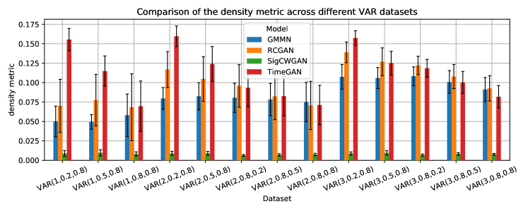
Figure D.1: Comparison of the performance on the density metric across all algorithms and benchmarks.

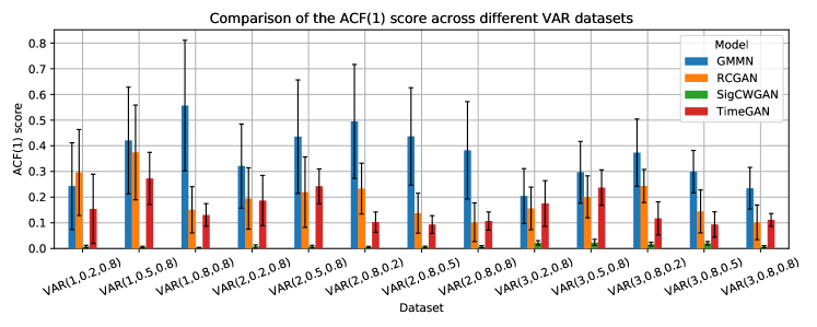
Figure D.2: Comparison of the performance on the absolute difference of lag-1 autocorrelation across all algorithms and benchmarks.

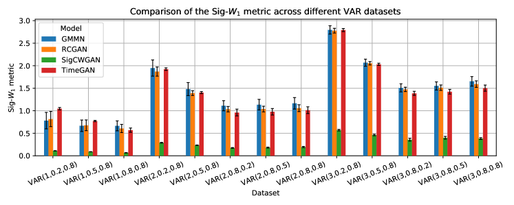
Figure D.3: Comparison of the performance on the Sig-$W_{1}$ metric across all algorithms and benchmarks.

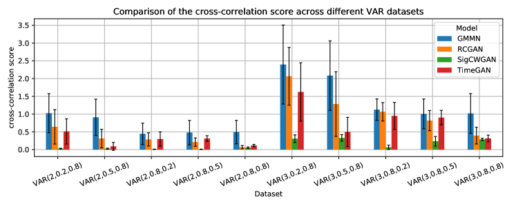
Figure D.4: Comparison of the performance on the cross-correlation metric across all algorithms and benchmarks.

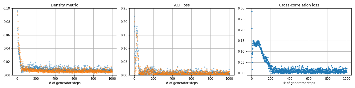
(a) SigCWGAN

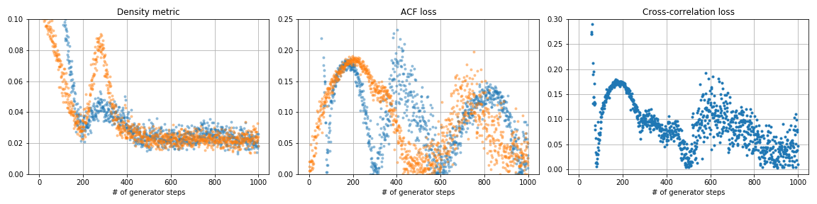
(b) TimeGAN

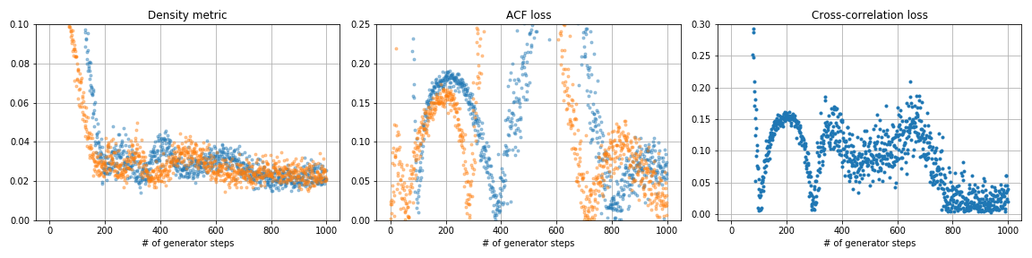
(c) RCGAN

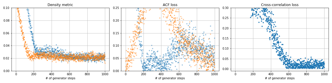
(d) GMMN

Figure D.5: Exemplary development of the considered distances and score functions during training for the $2$-dimensional $\operatorname{VAR}(1)$ model with autocorrelation coefficient $\phi=0.8$ and co-variance parameter $\sigma=0.8$. The colours blue and orange indicate the relevant distance / score for each dimension.

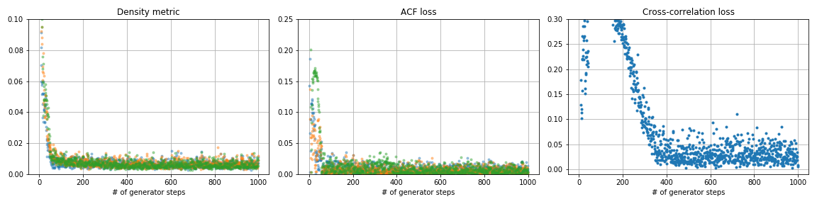
(a) SigCWGAN

(b) TimeGAN

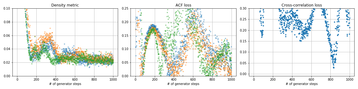
(c) RCGAN

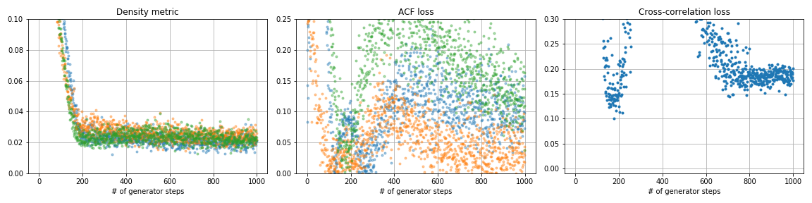
(d) GMMN

Figure D.6: Exemplary development of the considered distances and score functions during training for the $3$-dimensional $\operatorname{VAR}(1)$ model with autocorrelation coefficient $\phi=0.8$ and co-variance parameter $\sigma=0.8$. The colours blue, orange and green indicate the relevant distance / score for each dimension.

D.2 ARCH(p)

We implement extensive experiments on ARCH(p) with different $p-$lag values, i.e. $p\in\{2,3,4\}$. We choose the optimal degree of signature 3. The numerical results are summarized in Table D.4. The best results among all the models are highlighted in bold.

Table D.4: Numerical results of the ARCH(p) datasets.

Settings	$p=2$	$p=3$	$p=4$
Metric on marginal distribution
SigCWGAN	0,00918	0,00880	0.01142
TimeGAN	0,02569	0,02119	0.2191
RCGAN	0,01069	0,01612	0.01182
GMMN	0,00744	0,00783	0.01259
Absolute difference of lag-1 autocorrelation
SigCWGAN	0,00542	0,00852	0.01106
TimeGAN	0,01714	0,02401	0.03267
RCGAN	0,05372	0,01685	0.04879
GMMN	0,02056	0,00859	0.01441
$L_{1}$-norm of real and generated cross correlation matrices
SigCWGAN	0,00462	0,00546	0.00489
TimeGAN	0,00315	0,06551	0.04408
RCGAN	0,01604	0,08823	0.00235
GMMN	0,04326	0,03930	0.01603
$R^{2}$ obtained from TSTR. (TRTR first row.)
TRTR	0,32168	0,32615	0.33305
SigCWGAN	0,31623	0,31913	0.31642
TimeGAN	0,30835	0,30556	0.30240
RCGAN	0,31146	0,30727	0.30924
GMMN	0,27982	0,28072	0.30742
Sig-$W_{1}$ distance
SigCWGAN	0,12210	0,14682	0.14098
TimeGAN	0,20228	0,22761	0.23398
RCGAN	0,18781	0,20943	0.21876
GMMN	0,26797	0,26853	0.25811

D.3 SPX and DJI dataset

We provide the supplementary results on the SPX and DJI dataset. The summary of test metrics of different models is given by Table D.5. The test metrics over the training process of each method on (1) SPX dataset and (2) SPX and DJI dataset can be found in Figure D.7 and Figure D.8. The fitting of different models in terms of the cross-correlation matrix of the log-return and log-realized volatility of SPX are presented in Figure D.9.

Table D.5: Numerical results of the stocks datasets.

Data type	SPX	SPX + DJI
Metric on marginal distribution
SigCWGAN	0.0142	0.0093
CWGAN	0.0111	0.0151
TimeGAN	0.0089	0.0156
RCGAN	0.0088	0.0140
GMMN	0.0107	0.0181
Absolute difference of lag-1 autocorrelation
SigCWGAN	0.0302	0.0447
CWGAN	0.1617	0.0571
TimeGAN	0.0180	0.0232
RCGAN	0.0350	0.0515
GMMN	0.0273	0.0106
$L_{1}$-norm of real and generated cross correlation matrices
SigCWGAN	0.0503	0.0747
CWGAN	0.0131	0.3908
TimeGAN	0.0793	0.5401
RCGAN	0.0654	0.3959
GMMN	0.0409	0.2103
$R^{2}$ obtained from TSTR. (TRTR first row.)
TRTR	0.3689	0.3731
SigCWGAN	0.3576	0.3466
CWGAN	0.2744	0.2694
TimeGAN	0.3551	0.3602
RCGAN	0.3037	0.3532
GMMN	0.3375	0.3368
Sig-$W_{1}$ distance
SigCWGAN	0.0985	0.1307
CWGAN	0.1684	0.2881
TimeGAN	0.1265	0.2321
RCGAN	0.1462	0.2353
GMMN	0.1257	0.2448

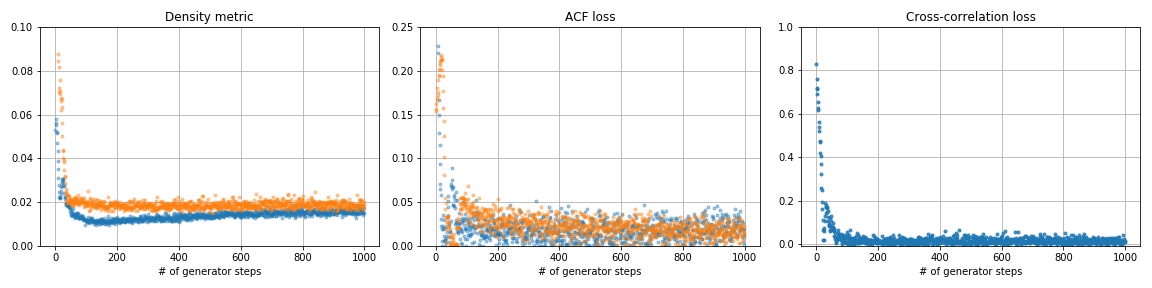
(a) SigCWGAN

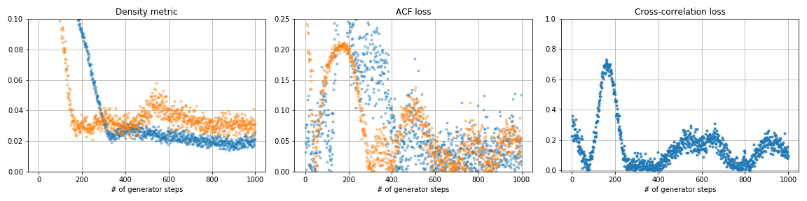
(b) TimeGAN

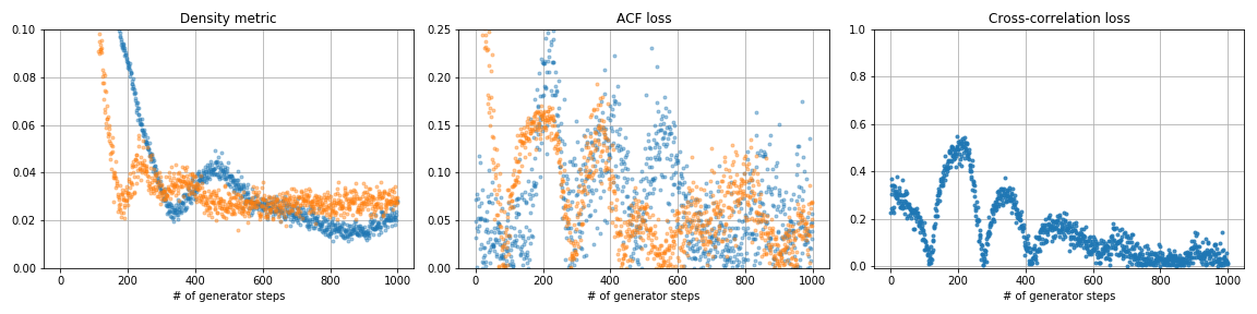
(c) RCGAN

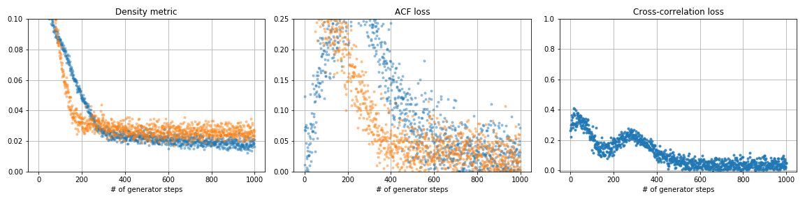
(d) GMMN

Figure D.7: Exemplary development of the considered distances and score functions during training for SPX data.

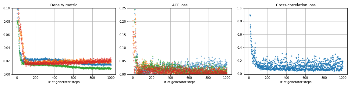
(a) SigCWGAN

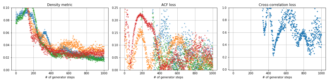
(b) TimeGAN

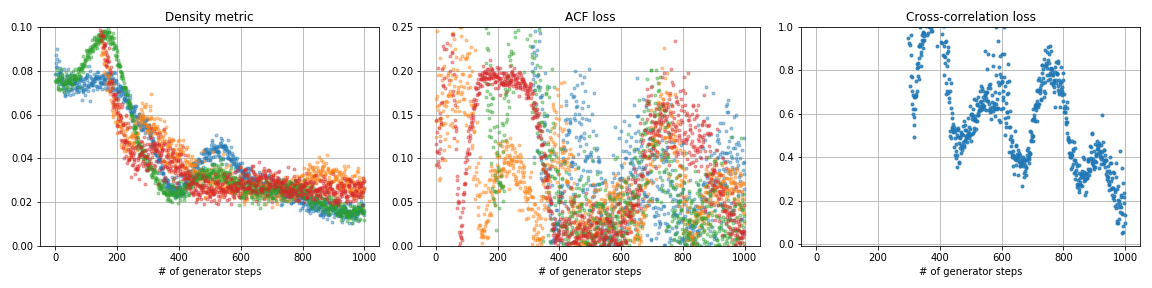
(c) RCGAN

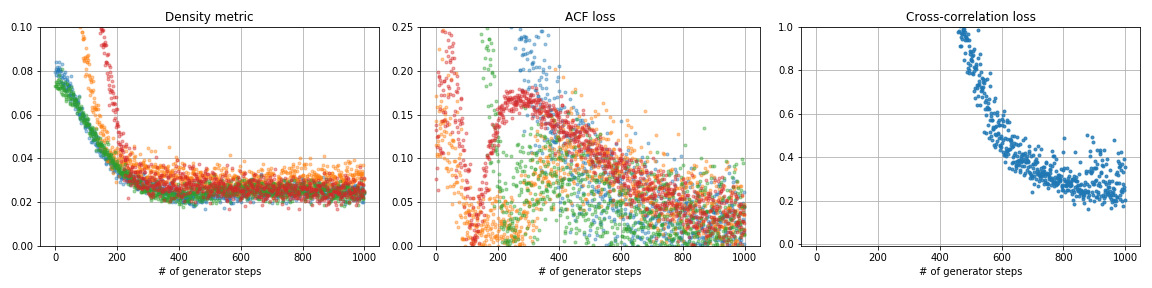
(d) GMMN

Figure D.8: ExemplARCHry development of the considered distances and score functions during training for SPX and DJI data.

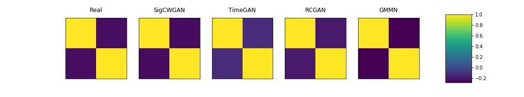
Figure D.9: Comparison of real and synthetic cross-correlation matrices for SPX data. On the far left the real cross-correlation matrix from SPX log-return and log-volatility data is shown. $x$/$y$-axis represents the feature dimension while the color of the $(i,j)^{th}$ block represents the correlation of $X_{t}^{(i)}$ and $X_{t}^{(j)}$. The colorbar on the far right indicates the range of values taken. Observe that the historical correlation between log-returns and log-volatility is negative, indicating the presence of leverage effects, i.e. when log-returns are negative, log-volatility is high.

	1	2	4	6	8
SigCWGAN	2.996, 7.948	3.510, 5.928	3.801, 7.439	3.944, 9.103	5.534, 10.742
TimeGAN	5.955, 8.586	8.470, 9.925	10.838, 14.816	13.163, 20.139	16.922, 22.870
RCGAN	2.788, 7.190	3.701, 5.425	5.090, 9.407	6.033, 12.424	9.380, 16.599
GMMN	9.049, 7.384	11.275, 9.150	19.302, 14.466	25.832, 21.690	28.269, 24.778
GARCH	104.776, 100.749	99.359, 109.313	103.137, 109.53	102.939, 107.669	102.527, 104.779

Table D.6: $R^{2}$ metric (%) of the stock datasets for different lag values. In each cell, the left/right number are the result for the SPX data/ the SPX and DJI data respectively.

	1	2	3	4	5
SigCWGAN	0.01342, 0.01192	0.02234, 0.02576	0.05744, 0.03592	0.07389, 0.08646	0.12571, 0.1057
TimeGAN	0.05792, 0.03035	0.06070, 0.03182	0.06823, 0.09887	0.05735, 0.10609	0.08387, 0.15083
RCGAN	0.03362, 0.04075	0.03134, 0.03977	0.06692, 0.08859	0.05641, 0.07687	0.09089, 0.11083
GMMN	0.01283, 0.02676	0.0177, 0.0253	0.04293, 0.06476	0.06740, 0.06952	0.09589, 0.09906
GARCH	0.4721, 0.4559	0.4661, 0.4741	0.6198,0.6282	0.7292,0.7312	0.8250,0.8212

Table D.7: Autocorrelation metric for the stock datasets for different lag values. In each cell, the left/right number are the result for the SPX data/ the SPX and DJI data respectively.

D.4 Bitcoin dataset

We provide the additional numerical results on the Bitcoin dataset as follows.

	1	2	3	4	5
SigCWGAN	0.0911	0.2814	0.3	0.3021	0.3028
TimeGAN	0.1203	0.2170	0.2312	0.2329	0.2568
RCGAN	0.0533	0.1486	0.15	0.1654	0.1751
GMMN	0.2093	0.3436	0.3448	0.3478	0.4333
GARCH	0.0872	0.1314	0.1378	0.1471	0.1501

Table D.8: Autocorrelation metric for the BTC dataset for different lag values

	1	2	4	6
SigCWGAN	0.3320	0.2681	0.3843	0.3128
TimeGAN	0.7582	0.5962	0.6394	0.6018
RCGAN	0.3165	0.2191	0.2898	0.2261
GMMN	0.3904	0.3436	0.2583	0.3426
GARCH	123.77	87.35	96.47	117.34

Table D.9: $R^{2}$ metric (%) of the BTC dataset for different lag values.

References

- Assefa et al. (2020) Samuel Assefa, Danial Dervovic, Mahmoud Mahfouz, Tucker Balch, Prashant Reddy, and Manuela Veloso. Generating synthetic data in finance: opportunities, challenges and pitfalls. 2020.
- Bellovin et al. (2019) Steven M Bellovin, Preetam K Dutta, and Nathan Reitinger. Privacy and synthetic datasets. Stan. Tech. L. Rev., 22:1, 2019.
- Boedihardjo and Geng (2014) Horatio Boedihardjo and Xi Geng. The uniqueness of signature problem in the non-markov setting. arXiv preprint arXiv:1401.6165, 2014.
- Boedihardjo et al. (2021) Horatio Boedihardjo, Joscha Diehl, Marc Mezzarobba, and Hao Ni. The expected signature of brownian motion stopped on the boundary of a circle has finite radius of convergence. Bulletin of the London Mathematical Society, 53(1):285–299, 2021.
- Buehler et al. (2020) Hans Buehler, Blanka Horvath, Terry Lyons, Imanol Perez Arribas, and Ben Wood. A data-driven market simulator for small data environments. Available at SSRN 3632431, 2020.
- Chevyrev and Kormilitzin (2016) Ilya Chevyrev and Andrey Kormilitzin. A primer on the signature method in machine learning. arXiv preprint arXiv:1603.03788, 2016.
- Chevyrev and Oberhauser (2022) Ilya Chevyrev and Harald Oberhauser. Signature moments to characterize laws of stochastic processes. The Journal of Machine Learning Research, 23(1):7928–7969, 2022.
- Chevyrev et al. (2016) Ilya Chevyrev, Terry Lyons, et al. Characteristic functions of measures on geometric rough paths. The Annals of Probability, 44(6):4049–4082, 2016.
- Cuchiero et al. (2020) Christa Cuchiero, Wahid Khosrawi, and Josef Teichmann. A generative adversarial network approach to calibration of local stochastic volatility models. Risks, 8(4):101, 2020.
- Daskalakis and Panageas (2018) Constantinos Daskalakis and Ioannis Panageas. The limit points of (optimistic) gradient descent in min-max optimization. arXiv preprint arXiv:1807.03907, 2018.
- Daskalakis et al. (2017) Constantinos Daskalakis, Andrew Ilyas, Vasilis Syrgkanis, and Haoyang Zeng. Training gans with optimism. arXiv preprint arXiv:1711.00141, 2017.
- Donahue et al. (2019) Chris Donahue, Julian J. McAuley, and Miller Puckette. Adversarial audio synthesis. In ICLR, 2019.
- Dudley (1989) Richard M Dudley. Real analysis and probability. wadsworth & brooks. Cole, Pacific Groves, California, 1989.
- Engel et al. (2019) Jesse Engel, Kumar Krishna Agrawal, Shuo Chen, Ishaan Gulrajani, Chris Donahue, and Adam Roberts. Gansynth: Adversarial neural audio synthesis. ArXiv, abs/1902.08710, 2019.
- Esteban et al. (2017) Cristóbal Esteban, Stephanie L. Hyland, and Gunnar Rätsch. Real-valued (medical) time series generation with recurrent conditional gans, 2017.
- Farnia and Ozdaglar (2020) Farzan Farnia and Asuman Ozdaglar. Gans may have no nash equilibria. arXiv preprint arXiv:2002.09124, 2020.
- Fawcett (2002) Thomas Fawcett. Problems in stochastic analysis: Connections between rough paths and non-commutative harmonic analysis. PhD thesis, University of Oxford, 2002.
- Fermanian (2022) Adeline Fermanian. Functional linear regression with truncated signatures. Journal of Multivariate Analysis, page 105031, 2022.
- Fu et al. (2019) Rao Fu, Jie Chen, Shutian Zeng, Yiping Zhuang, and Agus Sudjianto. Time series simulation by conditional generative adversarial net. arXiv preprint arXiv:1904.11419, 2019.
- Genevay et al. (2018) Aude Genevay, Lénaic Chizat, Francis Bach, Marco Cuturi, and Gabriel Peyré. Sample complexity of sinkhorn divergences. arXiv preprint arXiv:1810.02733, 2018.
- Gierjatowicz et al. (2020) Patryk Gierjatowicz, Marc Sabate-Vidales, David Siska, Lukasz Szpruch, and Zan Zuric. Robust pricing and hedging via neural sdes. Available at SSRN 3646241, 2020.
- Gulrajani et al. (2017) Ishaan Gulrajani, Faruk Ahmed, Martin Arjovsky, Vincent Dumoulin, and Aaron Courville. Improved training of wasserstein gans. arXiv preprint arXiv:1704.00028, 2017.
- Hambly and Lyons (2010) B.M. Hambly and Terry Lyons. Uniqueness for the signature of a path of bounded variation and the reduced path group. Annals of Mathematics,, 171(1):109–167, 2010.
- He et al. (2015) Kaiming He, Xiangyu Zhang, Shaoqing Ren, and Jian Sun. Delving deep into rectifiers: Surpassing human-level performance on imagenet classification. In Proceedings of the IEEE international conference on computer vision, pages 1026–1034, 2015.
- He et al. (2016) Kaiming He, Xiangyu Zhang, Shaoqing Ren, and Jian Sun. Deep residual learning for image recognition. In Proceedings of the IEEE conference on computer vision and pattern recognition, pages 770–778, 2016.
- Heber et al. (2009) Gerd Heber, Asger Lunde, Neil Shephard, and Kevin Sheppard. Oxford-man institute’s realized library, version 0.3, 2009.
- Heusel et al. (2017) Martin Heusel, Hubert Ramsauer, Thomas Unterthiner, Bernhard Nessler, and Sepp Hochreiter. Gans trained by a two time-scale update rule converge to a local nash equilibrium. In Advances in neural information processing systems, pages 6626–6637, 2017.
- Hyland et al. (2018) Stephanie Hyland, Cristóbal Esteban, and Gunnar Rätsch. Real-valued (medical) time series generation with recurrent conditional gans. 2018.
- Karatzas and Shreve (1998) Ioannis Karatzas and Steven E Shreve. Brownian motion. Springer, 1998.
- Kidger et al. (2019) Patrick Kidger, Patric Bonnier, Imanol Perez Arribas, Cristopher Salvi, and Terry Lyons. Deep signature transforms. In Advances in Neural Information Processing Systems, pages 3099–3109, 2019.
- Kingma and Ba (2014) Diederik P Kingma and Jimmy Ba. Adam: A method for stochastic optimization. arXiv preprint arXiv:1412.6980, 2014.
- Klüppelberg et al. (2004) Claudia Klüppelberg, Alexander Lindner, and Ross Maller. A continuous-time garch process driven by a lévy process: stationarity and second-order behaviour. Journal of Applied Probability, pages 601–622, 2004.
- Koochali et al. (2020) Alireza Koochali, Andreas Dengel, and Sheraz Ahmed. If you like it, gan it. probabilistic multivariate times series forecast with gan. arXiv preprint arXiv:2005.01181, 2020.
- Koshiyama et al. (2019) Adriano Koshiyama, Nick Firoozye, and Philip Treleaven. Generative adversarial networks for financial trading strategies fine-tuning and combination. arXiv preprint arXiv:1901.01751, 2019.
- Levin et al. (2013) Daniel Levin, Terry Lyons, and Hao Ni. Learning from the past, predicting the statistics for the future, learning an evolving system. arXiv preprint arXiv:1309.0260, 2013.
- Li and Ni (2022) Siran Li and Hao Ni. Expected signature of stopped Brownian motion on d-dimensional -domains has finite radius of convergence everywhere: . Journal of Functional Analysis, 282(12):109447, 2022.
- Li et al. (2015) Yujia Li, Kevin Swersky, and Rich Zemel. Generative moment matching networks. In International Conference on Machine Learning, pages 1718–1727, 2015.
- Lin et al. (2020) Tianyi Lin, Chi Jin, and Michael Jordan. On gradient descent ascent for nonconvex-concave minimax problems. In International Conference on Machine Learning, pages 6083–6093. PMLR, 2020.
- Liu et al. (2019) Xuanqing Liu, Tesi Xiao, Si Si, Qin Cao, Sanjiv Kumar, and Cho-Jui Hsieh. Neural sde: Stabilizing neural ode networks with stochastic noise. arXiv preprint arXiv:1906.02355, 2019.
- Lucic et al. (2017) Mario Lucic, Karol Kurach, Marcin Michalski, Sylvain Gelly, and Olivier Bousquet. Are gans created equal? a large-scale study. arXiv preprint arXiv:1711.10337, 2017.
- Lyons et al. (2015) Terry Lyons, Hao Ni, et al. Expected signature of brownian motion up to the first exit time from a bounded domain. The Annals of Probability, 43(5):2729–2762, 2015.
- Lyons et al. (2007) Terry J Lyons, Michael Caruana, and Thierry Lévy. Differential equations driven by rough paths. Springer, 2007.
- Mazumdar et al. (2019) Eric V Mazumdar, Michael I Jordan, and S Shankar Sastry. On finding local nash equilibria (and only local nash equilibria) in zero-sum games. arXiv preprint arXiv:1901.00838, 2019.
- Mertikopoulos et al. (2018) Panayotis Mertikopoulos, Christos Papadimitriou, and Georgios Piliouras. Cycles in adversarial regularized learning. In Proceedings of the Twenty-Ninth Annual ACM-SIAM Symposium on Discrete Algorithms, pages 2703–2717. SIAM, 2018.
- Mescheder et al. (2018) Lars Mescheder, Andreas Geiger, and Sebastian Nowozin. Which training methods for gans do actually converge? In International Conference on Machine learning (ICML), pages 3481–3490. PMLR, 2018.
- Ng and Jordan (2002) Andrew Y Ng and Michael I Jordan. On discriminative vs. generative classifiers: A comparison of logistic regression and naive bayes. In Advances in neural information processing systems, pages 841–848, 2002.
- Ni et al. (2021) Hao Ni, Lukasz Szpruch, Marc Sabate-Vidales, Baoren Xiao, Magnus Wiese, and Shujian Liao. Sig-wasserstein gans for time series generation. accepted by 2nd ACM International Conference on AI in Finance, 2021.
- Passeggeri (2020) Riccardo Passeggeri. On the signature and cubature of the fractional brownian motion for h¿12. Stochastic Processes and their Applications, 130(3):1226–1257, 2020. ISSN 0304-4149. doi: https://doi.org/10.1016/j.spa.2019.04.013. URL https://www.sciencedirect.com/science/article/pii/S0304414919302844.
- Ren et al. (2016) Yong Ren, Jun Zhu, Jialian Li, and Yucen Luo. Conditional generative moment-matching networks. In Advances in Neural Information Processing Systems, pages 2928–2936, 2016.
- Tsay (2005) Ruey S Tsay. Analysis of financial time series, volume 543. John wiley & sons, 2005.
- Tucker et al. (2020) Allan Tucker, Zhenchen Wang, Ylenia Rotalinti, and Puja Myles. Generating high-fidelity synthetic patient data for assessing machine learning healthcare software. NPJ digital medicine, 3(1):1–13, 2020.
- Wiese et al. (2019) Magnus Wiese, Lianjun Bai, Ben Wood, and Hans Buehler. Deep hedging: Learning to simulate equity option markets. SSRN Electronic Journal, 2019. ISSN 1556-5068. doi: 10.2139/ssrn.3470756. URL http://dx.doi.org/10.2139/ssrn.3470756.
- Wiese et al. (2020) Magnus Wiese, Robert Knobloch, Ralf Korn, and Peter Kretschmer. Quant gans: deep generation of financial time series. Quantitative Finance, pages 1–22, 2020.
- Xie et al. (2017) Zecheng Xie, Zenghui Sun, Lianwen Jin, Hao Ni, and Terry Lyons. Learning spatial-semantic context with fully convolutional recurrent network for online handwritten chinese text recognition. IEEE transactions on pattern analysis and machine intelligence, 40(8):1903–1917, 2017.
- Yang et al. (2017) Weixin Yang, Terry Lyons, Hao Ni, Cordelia Schmid, Lianwen Jin, and Jiawei Chang. Leveraging the path signature for skeleton-based human action recognition. arXiv preprint arXiv:1707.03993, 2017.
- Yoon et al. (2019) Jinsung Yoon, Daniel Jarrett, and Mihaela van der Schaar. Time-series generative adversarial networks. In Advances in Neural Information Processing Systems, pages 5509–5519, 2019.