Cost-effective Interactive Attention Learning with Neural Attention Process

Abstract

We propose a novel interactive learning framework which we refer to as Interactive Attention Learning (IAL), in which the human supervisors interactively manipulate the allocated attentions, to correct the model’s behavior by updating the attention-generating network. However, such a model is prone to overfitting due to scarcity of human annotations, and requires costly retraining. Moreover, it is almost infeasible for the human annotators to examine attentions on tons of instances and features. We tackle these challenges by proposing a sample-efficient attention mechanism and a cost-effective reranking algorithm for instances and features. First, we propose Neural Attention Process (NAP), which is an attention generator that can update its behavior by incorporating new attention-level supervisions without any retraining. Secondly, we propose an algorithm which prioritizes the instances and the features by their negative impacts, such that the model can yield large improvements with minimal human feedback. We validate IAL on various time-series datasets from multiple domains (healthcare, real-estate, and computer vision) on which it significantly outperforms baselines with conventional attention mechanisms, or without cost-effective reranking, with substantially less retraining and human-model interaction cost.

1 Introduction

Deep neural networks are arguably the most prevalent tools for predictive modeling tasks nowadays, thanks to their ability to learn complex functions with multiple layers of non-linear transformations. However, the complex nature of the model, at the same time, makes it difficult to interpret what they have learned, which has led to the recent surge of interest in interpretable models that are capable of providing interpretations of the model and the prediction in human-understandable forms (Gilpin et al., 2018).

Although recent works propose diverse solutions to interpretability (Choi et al., 2016; Ahmad et al., 2018; Lage et al., 2018), including attention mechanisms, activation visualization, and optimization for human-interpretability under human-in-the-loop, we face yet another challenge: not all machine-generated interpretations are correct or human understandable. This is mainly due to two reasons: 1) correctness and reliability of a learning model heavily depends on the quantity and quality of the training data. 2) neural networks tend to learn non-robust features that help with predictions but are not human-perceptible (Ilyas et al., 2019). Such unreliability of the interpretations is highly problematic for safety-critical applications such as clinical risk predictions (Ahmad et al., 2018; Sankar et al., 2019) or autonomous driving (Chi & Mu, 2017).

The main limitation of the existing models is that they mostly only consider passive roles for human supervisors, where they simply take the provided interpretations as is. Yet, a more effective way to use the interpretations is to use them as channels for human-model communications, such that the models learn by continuously interacting with the human supervisors, where they iteratively correct the model-generated interpretations. From a cognitive science perspective, human learning is done by internal reflection (back-propagation) and external explanation (human feedback) during social interactions (Clark et al., 2015).

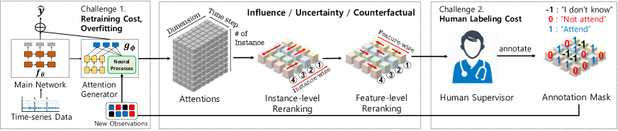
(A) Neural Attention Process

(B) Cost-Effective Re-ranking

(C) Human Annotation

Figure 1: Our Interactive Attention Learning (IAL) framework. IAL is an interactive learning framework which iteratively learns by interacting with the human supervisor, via the learned attentions. It allows efficient model update using (A) Neural Attention Process which does not require retraining, and cost-effective interaction via (B) Cost-effective reranking of the instances and features.

Based on this motivation, we propose an interactive learning framework, where the model learns by iteratively interacting with the human supervisors who manipulate the model by adjusting the provided interpretations, which is depicted in Figure 1. The specific interpretation mechanism we consider in this work is the attention mechanism (Bahdanau et al., 2014). While active learning asks for supervision at the instance level, in our interactive learning model, it asks for supervision at the attention level. However, this leads to multiple challenges regarding efficiency, which hinders their applications to practical scenarios:

• Model retraining cost and overfitting: To reflect human feedback, the model needs to be retrained, which is costly. Moreover, retraining the model with scarce human feedback may result in the model overfitting.

• Expensive human supervision cost: Obtaining human feedback on datasets with large numbers of training instances and features is extremely costly. Further, obtaining feedback on already correct interpretations is wasteful.

To tackle these practical challenges, we propose a novel interactive learning framework, which we refer to as Interactive Attention Learning (IAL), that allows both efficient model retraining and sample-efficient learning that minimizes human supervision cost. IAL consists of two main components: 1) Neural Attention Processes (NAP) and 2) Cost-Effective instance and feature Reranking (CER). Basically, our model minimizes retraining cost via NAP which allows the model to correct its attention-generating behaviour in a sample-efficient manner by incorporating new labeled instances without retraining. NAP also prevents overfitting, which is inevitable with scarce human feedbacks when using a conventional attention mechanism. Secondly, to address the expensive human labeling cost, CER reranks the instances, features, and timesteps (for time-series data) by their negative impacts. This enables the model to minimize human interaction cost, such that the human supervisors only correct the interpretations that are likely to be incorrect and influential to the prediction. The importance of each sample and feature is measured either by the uncertainty, influence function (Cook & Weisberg, 1980), or counterfactual estimation.

We validate our IAL framework on a variety of real world tasks with time-series data, including cerebral infarction risk prediction from electronic health records (EHR), New York City real-estate price forecast, and squat-posture prediction task. The experimental results show that our model outperforms baseline interactive learning schemes with significant margins, with considerably smaller interaction cost in terms of both model retraining and human annotation cost. Our contributions are as follows:

• We propose a novel interactive learning framework which iteratively updates the model by interacting with the human supervisor via the generated attentions.

• To minimize the retraining cost, we propose a novel probabilistic attention mechanism which sample-efficiently incorporates new attention-level supervisions on-the-fly without retraining and overfitting.

• To minimize human supervision cost, we propose an efficient instance and feature reranking algorithm, that prioritizes them based on their negative impacts on the prediction, measured either by uncertainty, influence function, or counterfactual estimation.

• We validate our model on five real-world datasets with binary, multi-label classification, and regression tasks, and show that our model obtains significant improvements over baselines with substantially less retraining and human feedback cost.

2 Related work

Interpretable machine learning

The literature on interpretable machine learning is vast, but we only discuss a few. A popular approach to obtain interpretable model is to build a simple proxy model that mimics the (local) behaviours of a complex model, using either simplified linear models (Ribeiro et al., 2016) or decision trees (Sato & Tsukimoto, 2001; Salzberg, 1994). Another approach, specific for neural networks, is analyzing their learned representations (Sharif Razavian et al., 2014; Yosinski et al., 2014) at each unit via visualization.  Bau et al. (2017) further consider interpretability of representations in light of their correspondence to semantic concepts, and utilize it for controlling the behaviours of generative adversarial networks (Bau et al., 2019). In this work, we propose a novel interactive learning framework that leverages the model’s interpretation to iteratively correct the model’s behaviour, while minimizing the interaction cost.

Attention Mechanism

Attention mechanism (Bahdanau et al., 2014) is an effective approach to adaptively select a subset of features in an input-dependent manner, such that the model dynamically focuses on more relevant features for prediction. This mechanism works by input-adaptively generating coefficients for input features to allocate more weights to more relevant features for prediction. Attention mechanisms have achieved success with various applications, including image translation (Xu et al., 2015), natural language understanding (Bahdanau et al., 2015; Vaswani et al., 2017), and visual question answering (Das et al., 2017). However, in the interactive learning setting, conventional attention mechanisms are either not trainable, or require retraining of the attention generator on the newly delivered attention-level annotations, which may lead to performance degeneration due to catastrophic forgetting. In this work, we incorporate benefits from the nonparametric and amortized inference of Neural Process (NPs) (Garnelo et al., 2018) into an attention mechanism such that it generalizes well with scarce human labels in a semi-supervised manner and can incorporate new labeled instances without retraining via an approximation of stochastic process.

Active learning

While there are vast literature on annotation methodology and active learning (Tong, 2001; Sener & Savarese, 2017), we here discuss a few relevant pre-existing works for learning from rationales, which is a popular annotation technique in natural language processing (Zaidan & Eisner, 2008) and vision (Donahue & Grauman, 2011), where a human highlights the important region of input. However, while these works directly zero out or modify input features, the attention generator in IAL provides its interpretation in the form of the attention, and the human supervisor corrects them. Furthermore, in conventional active learning settings, annotators’ roles are relatively passive, as they simply provide labels to each given instance such that they can’t see the effect of one’s annotation. However, the annotators in IAL actively interpret the generated attentions, directly modify the learning manifold of the model by masking them, and can immediately see the effect of the newly added annotation.

3 Interactive Attention Learning

Suppose we have a pre-trained neural network $\mathbf{F}_{{\bm{\Theta}}}$ with a parameter ${\bm{\Theta}}$ trained on a dataset $\mathcal{D}_{\text{train}}=\{(\mathbf{x}_{i}^{{\scriptscriptstyle{(1:T)}}},\mathbf{y}_{i})\}_{i=1}^{N}$. $\mathbf{x}_{i}^{{\scriptscriptstyle{(1:T)}}}=[\mathbf{x}_{i}^{{\scriptscriptstyle{(1)}}},\dots,\mathbf{x}_{i}^{{\scriptscriptstyle{(T)}}}]$ is a time-series instance with $\mathbf{x}_{i}^{{\scriptscriptstyle{(t)}}}\in^{D}$, and $\mathbf{y}_{i}\in^{L}$ is the corresponding label. We denote each labeled instance as $\mathbf{u}_{i}=(\mathbf{x}_{i}^{{\scriptscriptstyle{(1:T)}}},\mathbf{y}_{i})$. ${\bm{\Theta}}$ is trained to minimize the empirical risk, the expectation of individual loss $\mathcal{L}({\bm{\Theta}},\mathbf{u}_{i})$ over all training instances; we use mean-squared error for regressions or the categorical cross-entropy for classification problems. We further assume that ${\bm{\Theta}}$ consists of two sub-parameters $({\bm{\theta}},{\bm{\phi}})$, where ${\bm{\theta}}$ corresponds to the parameter of the main neural network $\mathbf{f}_{\bm{\theta}}$ and ${\bm{\phi}}$ corresponds to the parameter of the attention-generating network $\mathbf{g}_{\bm{\phi}}$. $\mathbf{g}_{\bm{\phi}}$ generates an attention ${\bm{\alpha}}^{{\scriptscriptstyle{(1:T)}}}_{i}$ for $\mathbf{x}_{i}^{{\scriptscriptstyle{(1:T)}}}$, where each ${\bm{\alpha}}^{{\scriptscriptstyle{(t)}}}_{i}$ is separated into an attention for time-axis $\beta^{{\scriptscriptstyle{(1:T)}}}_{i}$ and an attention for feature-axis ${\bm{\gamma}}^{{\scriptscriptstyle{(1:T)}}}_{i}$ (see (6) for detailed definition). The attentions are applied to the $D$ features along $T$ time-steps, and let the model focus on a specific features of the representations of inputs relevant to the prediction. Hence, the attention provides an interpretation of the model’s decision.

Our goal in this paper is to correct the behaviour of the attention-generating network $\mathbf{g}_{\bm{\phi}}$ with human supervision. This may be done by incrementally retraining $\mathbf{g}_{\bm{\phi}}$ over multiple rounds, where for each round human supervisors inspect the attentions generated by $\mathbf{g}_{\bm{\phi}}$ and update $\bm{\phi}$. We assume that a human supervisor provides an attention mask $\mathbf{m}^{{\scriptscriptstyle{(1:T)}}}_{i}$ for each sample $\mathbf{x}^{{\scriptscriptstyle{(1:T)}}}_{i}$ as ground-truth label, after manually examining the attention ${\bm{\alpha}}^{{\scriptscriptstyle{(1:T)}}}_{i}$ produced by $\mathbf{g}_{\bm{\phi}}$. An attention mask for a certain axis is defined to be a ternary value $\{-1,0,1\}$, where $-1$ indicates "I don’t know", $0$ indicates "Not attend", and $1$ indicates "Attend". Note that a naïve retraining of $\mathbf{g}_{\bm{\phi}}$ leads to the costly retraining of $\mathbf{f}_{\bm{\theta}}$ via gradient back-propagation. Instead, we choose to fix ${\bm{\theta}}$ and update $\bm{\phi}$ only to minimize the cost of retraining. We refer to this general framework that learns by interacting with the human supervisor via learned attention, as Interactive Attention Learning framework (IAL).

Algorithm 1 Interactive Attention Learning Framework

Input: $\mathcal{D}_{\text{train}}=\{\mathbf{x}_{i}^{{\scriptscriptstyle{(1:T)}}},\mathbf{y}_{i}\}_{i=1}^{N}$, $\bm{\Theta}=\{\bm{\theta},\bm{\phi}\}$, rounds $S$.
Output: $\bm{\Theta}$.

1:  Pretrain ${\bm{\Theta}}^{{\scriptscriptstyle{(0)}}}=\operatornamewithlimits{argmin}_{{\bm{\Theta}}}\mathcal{L}({\bm{\Theta}},\mathcal{D}_{\text{train}})+\Omega({\bm{\Theta}})$.

2:  for $s=1,...,S$ do

3:    $\mathcal{D}_{\text{selection}}^{{\scriptscriptstyle{(s)}}},\{{\bm{\alpha}}^{{\scriptscriptstyle{(1:T)}}}_{k}\}_{k=1}^{K}=\mathrm{CER}({\bm{\Theta}}^{{\scriptscriptstyle{(s-1)}}})$. $\quad\quad\triangleright$ Cost-Effective Re-ranking (CER)

4:    $\{\mathbf{m}^{{\scriptscriptstyle{(1:T)}}}_{k}\}^{K}_{k=1}=\mathrm{Evaluate}(\mathcal{D}_{\text{selection}}^{(s)},\{\bm{\alpha}^{{\scriptscriptstyle{(1:T)}}}_{k}\}_{k=1}^{K})$        $\triangleright$ Get attention masks for $\bm{\alpha}$

5:    ${\bm{\phi}}^{{\scriptscriptstyle{(s)}}}=\mathrm{NAP}(\mathcal{D}_{\text{selection}}^{(s)},\{\mathbf{m}^{{\scriptscriptstyle{(1:T)}}}_{k}\}^{K}_{k=1},\bm{\phi}^{{\scriptscriptstyle{(s-1)}}})$       $\triangleright$ Learn human feedback with quick forward        pass using Neural Attention Process (NAP).

6:    if $s=1$ then

7:       Retrain ${\bm{\Theta}}^{{\scriptscriptstyle{(1)}}}=\operatornamewithlimits{argmin}_{\bm{\Theta}}\mathcal{L}({\bm{\Theta}},\mathcal{D}_{\text{train}})+\Omega({\bm{\Theta}})$ with an adapted network containing NAP.

8:    end if

9:  end for

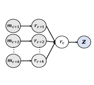
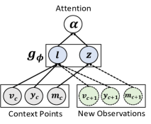
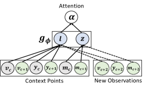
(a) Neural Attention Process (NAP)	(b) First Round ($s$=1)	(c) Further Rounds ($s$=2,3,..)

Figure 2: (a): NAP naturally reflects the information from the annotation summarization $\mathbf{z}$ via amortization. (b) For new observations (annotation mask $\mathbf{m}_{c+1}$), NAP accepts them as input and generates the mean and variance parameter for $\mathbf{z}$. (c) NAP doesn’t require retraining for further new observations, in that NAP automatically adapt to them at the cost of a forward pass through a network $\mathbf{g}_{\bm{\phi}}$.

Yet, as discussed in the introduction, there are still remaining challenges that need to be tackled. First, the retraining of $\mathbf{g}_{\bm{\phi}}$ will still incur a non-negligible cost and may also result in overfitting when human feedback is scarce. To tackle this, we propose a novel attention generator that can readily incorporate human annotations without retraining. Another challenge is reducing the human interaction cost. Ideally, a human annotator may have a look on the entire attentions generated by $\mathbf{g}_{\bm{\phi}}$. This involves examining all instances $(\mathbf{u}_{i},\dots,\mathbf{u}_{N})$, and within each instance, all features over all time-steps $(\mathbf{u}_{i,1}^{(1)},\dots,\mathbf{u}_{i,D}^{(T)})$. This is not feasible and wasteful since many attention values are already correct. To tackle this problem, we further propose a cost-effective reranking method which prioritizes the instances and features by their impacts on the model’s prediction, to maximize performance gains with minimal human effort.

Algorithm 1 describes the detailed algorithm for our IAL framework that leverages the proposed attention mechanism and re-ranking method. In the next two subsections, we describe the two components that minimize both the model retraining cost and human-model interaction cost.

3.1 Neural Attention Process

In this section, we describe Neural Attention Process (NAP), an novel attention generator based on NPs (Garnelo et al., 2018). NAP can effectively update the model without retraining by amortization using sparse human annotations.

Before describing our approach, we briefly explain how attention is applied for time-series prediction, using RETAIN (Choi et al., 2016) as our base model. Let $\mathbf{v}^{{\scriptscriptstyle{(1:T)}}}=\mathbf{W}_{\text{emb}}\mathbf{x}^{{\scriptscriptstyle{(1:T)}}}$ be a linear embedding of an input. We restrict $\mathbf{v}^{{\scriptscriptstyle{(1:T)}}}$ to have the same dimensionality $(D)$ as $\mathbf{x}^{{\scriptscriptstyle{(1:T)}}}$, so that we can directly compute the contribution of a certain feature to a prediction. The model computes attention coefficients for both time-steps and input-features as,

$$\mathbf{o}^{{\scriptscriptstyle{(1:T)}}}=\operatorname{RNN}_{\beta}(\mathbf{v}^{{\scriptscriptstyle{(1:T)}}}),$$ (1)

$$\mathbf{h}^{{\scriptscriptstyle{(1:T)}}}=\operatorname{RNN}_{\bm{\gamma}}(\mathbf{v}^{{\scriptscriptstyle{(1:T)}}}),$$ (2)

$$e^{{\scriptscriptstyle{(t)}}}=\mathbf{w}_{\beta}^{\top}\mathbf{o}^{{\scriptscriptstyle{(t)}}}+b_{\beta}\text{ for }t=1,\dots,T,$$ (3)

$$\mathbf{q}^{{\scriptscriptstyle{(t)}}}=\mathbf{W}_{\bm{\gamma}}\mathbf{h}^{{\scriptscriptstyle{(t)}}}+\mathbf{b}_{\bm{\gamma}}\text{ for }t=1,\dots,T,$$ (4)

$$\beta^{{\scriptscriptstyle{(1:T)}}}=\operatorname{Softmax}(e^{{\scriptscriptstyle{(1)}}},\dots,e^{{\scriptscriptstyle{(T)}}}),$$ (5)

$${\bm{\gamma}}^{{\scriptscriptstyle{(t)}}}=\tanh(\mathbf{q}^{{\scriptscriptstyle{(t)}}})\text{ for }t=1,\dots,T.$$ (6)

Here, $\beta^{{\scriptscriptstyle{(1:T)}}}$ are attention weights applied for time-steps and ${\bm{\gamma}}^{{\scriptscriptstyle{(1:T)}}}$ are attention weights for the input features. We may also consider the stochastic attention as in (Xu et al., 2015). Given $\bm{\alpha}^{{\scriptscriptstyle{(1:T)}}}=\{\beta^{{\scriptscriptstyle{(1:T)}}},{\bm{\gamma}}^{{\scriptscriptstyle{(1:T)}}}\}$, the model makes predictions as $\hat{\mathbf{y}}=\mathbf{h}(\sum_{t=1}^{T}\beta^{{\scriptscriptstyle{(t)}}}\cdot({\bm{\gamma}}^{{\scriptscriptstyle{(t)}}}\odot\mathbf{v}^{{\scriptscriptstyle{(t)}}}))$ where $\odot$ is the element-wise multiplication and $\mathbf{h}$ is an output layer.

Now we describe NAP, especially how it amortizes the procedure of updating the model given human annotations. Let $\{\mathbf{m}_{k}^{{\scriptscriptstyle{(1:T)}}}\}_{k=1}^{K}$ be a set of attention masks given by human annotators for a subset $\mathcal{D}_{\text{selection}}=\{(\mathbf{x}_{k}^{{\scriptscriptstyle{(1:T)}}},\mathbf{y}_{k})\}_{k=1}^{K}\subseteq\mathcal{D}_{\text{train}}$ with $K\ll N$. Instead of exhaustively retraining $\mathbf{g}_{\bm{\phi}}$, NAP learns to summarize $\mathcal{D}_{\text{selection}}$ to a latent vector, and give the summarization as an additional input to the attention generating network. This approach, when trained properly, can automatically adapt to new annotations without having to retrain the parameters. From below, we describe the components of NAP in more detail.

Embedding & summarizing the annotations

We first feed the input embedding $\mathbf{v}^{{\scriptscriptstyle{(1:T)}}}$ to LSTM (Hochreiter & Schmidhuber, 1997) ($\mathrm{RNN}_{\beta},\mathrm{RNN}_{\bm{\gamma}}$) to generate time-series representation $\mathbf{l}^{{\scriptscriptstyle{(1:T)}}}=[\mathbf{\mathbf{o}}^{{\scriptscriptstyle{(1:T)}}},\mathbf{h}^{{\scriptscriptstyle{(1:T)}}}]$. Given attention masks $\{\mathbf{m}_{k}^{{\scriptscriptstyle{(1:T)}}}\}_{k=1}^{K}$, we build an intermediate representation $\{\mathbf{r}^{{\scriptscriptstyle{(1:T)}}}_{k}\}_{k=1}^{K}$ via another LSTM. Then, for each time step, we build a summarized representation $\bar{\mathbf{r}}^{{\scriptscriptstyle{(t)}}}$ by a permutation-invariant operation (for instance, average),

$$\small\bar{\mathbf{r}}^{{\scriptscriptstyle{(t)}}}=\mathbf{r}^{{\scriptscriptstyle{(t)}}}_{1}\oplus\dots\oplus\mathbf{r}^{{\scriptscriptstyle{(t)}}}_{K}.$$ (7)

Having $\bar{\mathbf{r}}^{{\scriptscriptstyle{(1:T)}}}$, we define a distribution for the summary variable $\mathbf{z}$ as Gaussian:

$$\mathbf{z}^{{\scriptscriptstyle{(t)}}}\sim\mathcal{N}(\bm{\mu}(\bar{\mathbf{r}}^{{\scriptscriptstyle{(t)}}}),\bm{\sigma}^{2}(\bar{\mathbf{r}}^{{\scriptscriptstyle{(t)}}})),$$ (8)

$$\bm{\mu}(\bar{\mathbf{r}}^{{\scriptscriptstyle{(t)}}})=\mathbf{W}_{\bm{\mu}}\bar{\mathbf{r}}^{{\scriptscriptstyle{(t)}}}+\mathbf{b}_{\bm{\mu}},$$ (9)

$$\bm{\sigma}(\bar{\mathbf{r}}^{{\scriptscriptstyle{(t)}}})=\mathrm{softplus}(\mathbf{W}_{\bm{\sigma}}\bar{\mathbf{r}}^{{\scriptscriptstyle{(t)}}}+\mathbf{b}_{\bm{\sigma}}).$$ (10)

Generating attentions $\&$ Training NAP

Now we generate the attention by a similar procedure to (6), but instead of feeding only $\mathbf{l}^{{\scriptscriptstyle{(1:T)}}}=(\mathbf{o}^{{\scriptscriptstyle{(1:T)}}},\mathbf{h}^{{\scriptscriptstyle{(1:T)}}})$, we feed both $\mathbf{l}^{{\scriptscriptstyle{(1:T)}}}$ and the annotation summarization vector $\mathbf{z}^{{\scriptscriptstyle{(1:T)}}}$ by concatenation. This allows the network to naturally reflect the information obtained from $\mathbf{z}^{{\scriptscriptstyle{(1:T)}}}$ without having to retrain the whole attention network parameter $\bm{\phi}$. The original NP is meta-trained using many training examples. Likewise, NAP requires a meta-training for adapting the attention generating network $\mathbf{g}_{\bm{\phi}}$ to take $\mathbf{z}^{{\scriptscriptstyle{(1:T)}}}$ as an additional input (Figure 2, (b)). We found that this adaptation requires significantly fewer training examples than the typical NP training, possibly because the network is pretrained using $\mathcal{D}_{\text{train}}$ in advance. For such adaptation training, given a set of annotated examples, we randomly subsample annotations for each training step to comprise a random task to meta-train the model. The subsampling prevents NAP from completely being over-fitted to the entire annotation set, leading to effective generalization to newly delivered annotations across rounds. We also regularize $\mathbf{z}^{{\scriptscriptstyle{(1:T)}}}$ by positing a standard Gaussian prior distribution as in Garnelo et al. (2018). We train the parameters of NAP via stochastic gradient variational inference.

3.2 Cost-Effective instance and feature Reranking

As we discussed earlier, letting human annotators inspect attentions for all instances and features is inefficient even for a small dataset. We may reduce this cost by randomly subsampling from all attention values, but it may result in selecting instances or features that are already correct or have little impact to the model’s prediction. Thus, we want to prioritize the attentions by their negative impact on the model’s prediction, such that each feedback given by the human supervisor results in large performance improvements. In this section, we propose a general framework, depicted in Figure 3, to select important instances and features. For instance-level selection, we use the influence score and uncertainty score. For feature-level, we use the influence score, uncertainty score, and counterfactual score.

3.2.1 Instance-level reranking

Influence score

We use the influence function (Koh & Liang, 2017) to approximate the impact of individual training points on the model prediction. The idea behind this is simple; given a validation point $\mathbf{u}^{\text{val}}$, how would the validation loss change if a certain training instance $\mathbf{u}$ is excluded from training procedure? Formally, let $\hat{\bm{\Theta}}$ be the minimizer of empirical risk for the original training set, $\frac{1}{N}\sum_{i=1}^{N}\mathcal{L}({\bm{\Theta}},\mathbf{u}_{i})$, and $\hat{\bm{\Theta}}_{-\mathbf{u}}$ be simply the one computed from empirical risk without $\mathbf{u}$, $\frac{1}{N-1}\sum_{\mathbf{u}_{i}\neq\mathbf{u}}\mathcal{L}({\bm{\Theta}},\mathbf{u}_{i})$. The effect of removing $\mathbf{u}$ is then measured as $\mathcal{L}(\hat{\bm{\Theta}}_{-\mathbf{u}},\mathbf{u}^{\text{val}})-\mathcal{L}(\hat{\bm{\Theta}}_{\mathbf{u}},\mathbf{u}^{\text{val}})$. Since exactly computing this involves $N$ retraining procedures and quite expensive, Koh & Liang (2017) propose to use the influence function $\mathcal{I}(\mathbf{u},\mathbf{u}^{\text{val}})$ to approximate it as follows:

$$\mathcal{L}(\hat{\bm{\Theta}}_{-\mathbf{u}},\mathbf{u}^{\text{val}})-\mathcal{L}(\hat{\bm{\Theta}},\mathbf{u}^{\text{val}})\approx-\frac{1}{N}\mathcal{I}(\mathbf{u},\mathbf{u}^{\text{val}}),$$ (11)

$$\mathcal{I}(\mathbf{u},\mathbf{u}^{\text{val}})\stackrel{{\scriptstyle\mathrm{def}}}{{=}}-\nabla_{\bm{\Theta}}\mathcal{L}(\mathbf{u}^{\text{val}},\hat{\bm{\Theta}})H^{-1}_{\hat{\bm{\Theta}}}\nabla_{{\bm{\Theta}}}\mathcal{L}(\mathbf{u},\hat{\bm{\Theta}}),$$ (12)

where $H_{\bm{\Theta}}=\frac{1}{N}\sum_{i=1}^{N}\nabla^{2}_{\bm{\Theta}}\mathcal{L}(\hat{\bm{\Theta}},\mathbf{u}_{i})$ is the Hessian. To summarize, the influence function $\mathcal{I}(\mathbf{u},\mathbf{u}^{\text{val}})$ approximates the change in the validation loss (up to a constant) without having to retrain the model.

During training, we are given a set of validation instances $\mathcal{D}_{\text{valid}}=\{\mathbf{u}^{\text{val}}_{j}\}_{j=1}^{M}$. Then, we first select $P$ instances that have the highest validation loss $\mathcal{L}(\hat{\bm{\Theta}},\mathbf{u}^{\text{val}}_{j})$ to comprise $\mathcal{D}^{\prime}_{\text{valid}}=\{\mathbf{u}^{\text{val}}_{p}\}_{p=1}^{P}$. The intuition behind is that we want to select the training instances having large impact on the validation instances that are mis-predicted by the current model. In the supplementary file, we empirically show that this indeed improves the performance. Having $\mathcal{D}^{\prime}_{\text{valid}}$, the influence score of a training instance $\mathbf{u}_{i}$ is computed as $\mathcal{I}(\mathbf{u}_{i})=\sum_{p=1}^{P}\mathcal{I}(\mathbf{u}_{i},\mathbf{u}^{\text{val}}_{p})$.

Uncertainty score

While influence scores provide direct measures of the negative impact of an instance, it is expensive because of the Hessian computation. An alternative, and less expensive approach to measure the negative impacts is using the uncertainty. We assume that instances having high-predictive uncertainties are potential candidate to be corrected. This is a common approach in active learning or Bayesian optimization literature, where the points with high-uncertainties are explored. Instance-level predictive uncertainty can simply be obtained by Monte-Carlo (MC) sampling (Gal & Ghahramani, 2016). We denote the instance-level uncertainty score as $\mathrm{Var}(\mathbf{u}_{i})$.

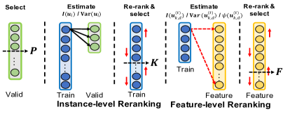
Figure 3: Cost-Effective Re-ranking Procedure (CER).

3.2.2 Feature-level reranking

Influence score

We can also estimate the feature-level influence score by a similar idea; if certain feature value is modified, how would the validation loss change? Let $\mathbf{u}=(\mathbf{x}^{{\scriptscriptstyle{(1:T)}}},\mathbf{y})$ be a training instance, and suppose we want to compute the influence of $\mathbf{u}_{i,d}^{(t)}$, which is the $d$-th input feature for timestep $t$, $x^{{\scriptscriptstyle{(t)}}}_{d}\in$. Define a perturbed data point $\mathbf{u}_{\delta}\stackrel{{\scriptstyle\mathrm{def}}}{{=}}(\mathbf{x}^{{\scriptscriptstyle{(1:T)}}}+\delta\mathbf{e}_{t,d},\mathbf{y})$ where $\mathbf{e}_{t,d}$ is an one-hot vector having $d$-th feature of $t$-th time step as one. Let $\hat{\bm{\Theta}}_{\mathbf{u}_{\delta},-\mathbf{u}}$ be the empirical risk minimizer with $\mathbf{u}$ replaced by $\mathbf{u}_{\delta}$. Then, as before, we have

$$\mathcal{L}(\hat{\bm{\Theta}}_{\mathbf{u}_{\delta},-\mathbf{u}},\mathbf{u}^{\text{val}})-\mathcal{L}(\hat{\bm{\Theta}},\mathbf{u}^{\text{val}})$$

$$\approx-\frac{1}{N}(\mathcal{I}(\mathbf{u}_{\delta},\mathbf{u}^{\text{val}})-\mathcal{I}(\mathbf{u},\mathbf{u}^{\text{val}})).$$ (13)

Based on this approximation, we sampled $\delta$ from mean $\pm$ 2$\cdot$std of features, and computed the average influence score over multiple perturbations to rank features. As for the instance-level influence score, we add up the influence scores for all selected validation samples. We denote $\mathcal{I}(\mathbf{u}_{i,d}^{{\scriptscriptstyle{(t)}}})$ the influence score obtained by perturbing $\mathbf{u}_{i,d}^{(t)}$.

Uncertainty score

NAP induces stochasticity to the attentions applied to the individual features, and this naturally leads to feature-level uncertainty scores. As for the instance-level uncertainty score, we computed variances of attentions applied for each feature by MC sampling. We denote the feature-level uncertainty score of $\mathbf{u}_{i,d}^{(t)}$ as $\mathrm{Var}(\mathbf{u}_{i,d}^{(t)})$.

Algorithm 2 Cost-Effective Re-ranking

Input: $\mathcal{D}_{\text{train}}=\{\mathbf{u}_{i}\}_{i=1}^{N}$, $\mathcal{D}_{\text{valid}}=\{\mathbf{u}^{\text{val}}_{j}\}_{j=1}^{M}$, $P$, $K$, $F$, $\bm{\Theta}^{{\scriptscriptstyle{(s-1)}}}$.
Output: $\mathcal{D}_{\text{selection}}^{{\scriptscriptstyle{(s)}}}=\{\mathbf{u}_{k}\}_{k=1}^{K}$, $\{{\bm{\alpha}}^{{\scriptscriptstyle{(1:T)}}}_{k}\}_{k=1}^{K}$.

1:  Evaluate the loss for $\mathcal{D}_{\text{valid}}$.

2:  Sort $\{\mathbf{u}^{\text{val}}_{j}\}_{j=1}^{M}$ in the descending order of $\mathcal{L}({\bm{\Theta}}^{{\scriptscriptstyle{(s-1)}}},\mathbf{u}^{\text{val}}_{j})$ and select top-$P$ valid points $\mathcal{D}^{\prime}_{\text{valid}}$.

3:  $\triangleright$ Instance-level re-ranking

4:  for $i=1,...,N$ do

5:    Compute the influence $\mathcal{I}(\mathbf{u}_{i})$ or uncertainty score $\mathrm{Var}(\mathbf{u}_{i})$.

6:    Select the top $K$-training points $\mathcal{D}_{\text{selection}}$ w.r.t the score.

7:  end for

8:  $\triangleright$ Feature-level re-ranking

9:  for $k=1,\dots,K$ do

10:    for $(t,d)=(1,1),\dots,(T,D)$ do

11:       Compute influence $\mathcal{I}(\mathbf{u}_{k,d}^{{\scriptscriptstyle{(t)}}})$ or uncertainty $\mathrm{Var}(\mathbf{u}_{k,d}^{{\scriptscriptstyle{(t)}}})$ or counterfactual $\psi(\mathbf{u}_{k,d}^{{\scriptscriptstyle{(t)}}})$ score.

12:       Select top-$F$ features.

13:    end for

14:  end for

Figure 4: Attention annotation interface (risk prediction for Cardiovascular Disease (CVD)) with counterfactual estimation tool.

Conterfactual score

The last score, which we call as counterfactual score, is the most direct measure of the negative impact of a feature. It answers the following question: how would the prediction change if we ignore a certain feature by manually turning off the corresponding attention value? This does not require retraining since we can simply set its attention value to zero, yet still effective because our goal is to rank the features w.r.t. their importance in attention feedback. Recall that given an attention $(\beta^{{\scriptscriptstyle{(1:T)}}},{\bm{\gamma}}^{{\scriptscriptstyle{(1:T)}}})$ generated from $\mathbf{g}_{\bm{\phi}}$, a prediction is given as

$$\small\hat{\mathbf{y}}_{i}=\mathbf{h}\bigg{(}\sum_{t=1}^{T}\beta_{i}^{{\scriptscriptstyle{(t)}}}{\bm{\gamma}}_{i}^{{\scriptscriptstyle{(t)}}}\odot\mathbf{v}^{{\scriptscriptstyle{(t)}}}_{i}\bigg{)},$$ (14)

where $\mathbf{v}_{i}^{{\scriptscriptstyle{(1:T)}}}$ is the linear embedding of $\mathbf{x}^{{\scriptscriptstyle{(1:T)}}}$. The effect of perturbing $\mathbf{u}_{i,d}^{(t)}$ can be then computed as follows:

$$\small\hat{\mathbf{y}}_{i,-(t,d)} =\mathbf{h}\bigg{(}\sum_{t^{\prime}\neq t}\beta_{i}^{{\scriptscriptstyle{(t^{\prime})}}}\gamma_{i}^{{\scriptscriptstyle{(t^{\prime})}}}\odot\mathbf{v}_{i}^{{\scriptscriptstyle{(t)}}}+\beta_{i}^{{\scriptscriptstyle{(t)}}}{\bm{\gamma}}_{i,-d}^{{\scriptscriptstyle{(t)}}}\odot\mathbf{v}_{i}^{{\scriptscriptstyle{(t)}}}\bigg{)}$$

$$\psi(\mathbf{u}_{i,d}^{{\scriptscriptstyle{(t)}}}) =\hat{\mathbf{y}}_{i}-\hat{\mathbf{y}}_{i,-(t,d)},\vspace{-0.01in}$$ (15)

where ${\bm{\gamma}}_{i,-d}^{{\scriptscriptstyle{(t)}}}$ is the attention where ${\bm{\gamma}}_{i,d}^{(t)}$ = 0. We empirically found that the counterfactual score is the most effective measure for feature-level reranking (See Table 2).

3.3 Human Annotation

Finally, given a subset selected using CER whose instances and features also sorted by their negative impacts, we visualize and present the attentions to human annotators, using an online interactive user interface. We provide an example of this interface in Figure 4 for the clinical risk prediction task. On the interface, the annotators set the attention mask for each feature to one of the following values: $\mathbf{m}_{k}=\{-1:\textit{I don't know},0:\textit{Not attend},1:\textit{Attend}\}$. The interface visually emphasizes the features with high attentions using either a bar plot (for tabular data) or an attention map (for image data) depending on the given task. Then, the annotators examine attention weights to check whether they are incorrectly allocated, and correct them when necessary.

		EHR			Fitness	Real Estate
		Heart Failure	Cerebral Infarction	CVD	Squat	Forecasting
One-time Training	RETAIN	0.6069 $\pm$ 0.01	0.6394 $\pm$ 0.02	0.6018 $\pm$ 0.02	0.8425 $\pm$ 0.03	0.2136 $\pm$ 0.01
	Random-RETAIN	0.5952 $\pm$ 0.02	0.6256 $\pm$ 0.02	0.5885 $\pm$ 0.01	0.8221 $\pm$ 0.05	0.2140 $\pm$ 0.01
	IF-RETAIN	0.6134 $\pm$ 0.03	0.6422 $\pm$ 0.02	0.5882 $\pm$ 0.02	0.8363 $\pm$ 0.03	0.2049 $\pm$ 0.01
Random Re-ranking	Random-UA	0.6231 $\pm$ 0.03	0.6491 $\pm$ 0.01	0.6112 $\pm$ 0.02	0.8521 $\pm$ 0.02	0.2222 $\pm$ 0.02
	Random-NAP	0.6414 $\pm$ 0.01	0.6674 $\pm$ 0.02	0.6284 $\pm$ 0.01	0.8525 $\pm$ 0.01	0.2061 $\pm$ 0.01
IAL (Cost-effective)	AILA	0.6363 $\pm$ 0.03	0.6602 $\pm$ 0.03	0.6193 $\pm$ 0.02	0.8425 $\pm$ 0.01	0.2119 $\pm$ 0.01
	IAL-NAP	0.6612 $\pm$ 0.02	0.6892 $\pm$ 0.03	0.6371 $\pm$ 0.02	0.8689 $\pm$ 0.01	0.1835 $\pm$ 0.01

Table 1: The binary $\&$ multi-class classification performance on the three electronic health records datasets and one fitness dataset. The reported numbers are mean-AUROC for EHR and mean-Accuracy for squat. In the real estate forecasting task, the number indicates mean-percentage error, meaning a lower error indicates better performance.

IAL-NAP Variants		EHR			Fitness	Real Estate
Instance-level	Feature-level	Heart Failure	Cerebral Infarction	CVD	Squat	Forecasting
Influence Function	Uncertainty	0.6563 $\pm$ 0.01	0.6821 $\pm$ 0.02	0.6308 $\pm$ 0.02	0.8712 $\pm$ 0.01	0.1921 $\pm$ 0.01
Influence Function	Influence Function	0.6514 $\pm$ 0.02	0.6825 $\pm$ 0.01	0.6329 $\pm$ 0.03	0.8632 $\pm$ 0.01	0.1865 $\pm$ 0.02
Influence Function	Counterfactual	0.6592 $\pm$ 0.02	0.6921 $\pm$ 0.03	0.6379 $\pm$ 0.02	0.8682 $\pm$ 0.01	0.1863 $\pm$ 0.02
Uncertainty	Counterfactual	0.6612 $\pm$ 0.01	0.6892 $\pm$ 0.03	0.6371 $\pm$ 0.02	0.8689 $\pm$ 0.02	0.1835 $\pm$ 0.02

Table 2: Results of Ablation study with proposed IAL-NAP combinations for instance- and feature-level reranking on all tasks.

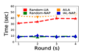
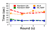
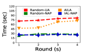
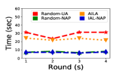
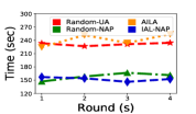
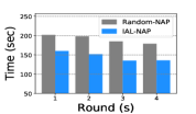
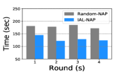
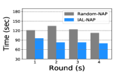
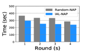
(a) Heart Failure	(b) Cerebral Infarction	(c) CVD	(d) Squat	(e) Real Estate

Figure 5: (top) Retraining Time to retrain examples of human annotation on all task for Random-UA, AILA, Random-NAP, and IAL-NAP. (bottom) mean Response Time (mean-RT) of human labeling on three risk prediction task, one squat posture classification task, and one realestate forecasting task (IAL-NAP with features ranked by uncertainty vs Random-NAP with features ranked randomly).

	Age	Smoking	SysBP	HDL	LDL
2009	31	Yes	139	54	97
2010	32	Yes	134	55	97
Current State	33 yrs	Yes	141 mmHg	55 mg/dL	102 mg/dL

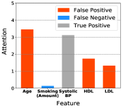
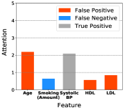
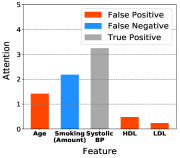
(a) Pretrained	(b) $s$=1	(c) $s$=2

Figure 6: Visualization of attention for a selected patient on Cardiovascular Disease (CVD) prediction task. Contribution indicates the extent to which each individual feature affects the onset of CVD in 1 year. Age - Age, Smoking - Whether currently smokes a cigarette, SysBP - Systolic blood pressure, HDL - High-density lipoproteins cholesterol, LDL - Low-density lipoprotein cholesterol. Bars correspond to attentions.

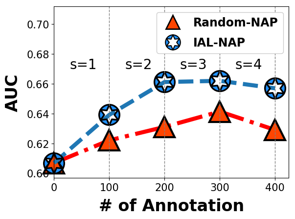
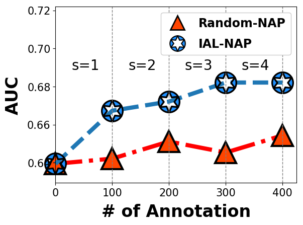
(a) Heart Failure	(b) Cerebral Infarction

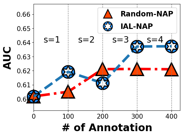
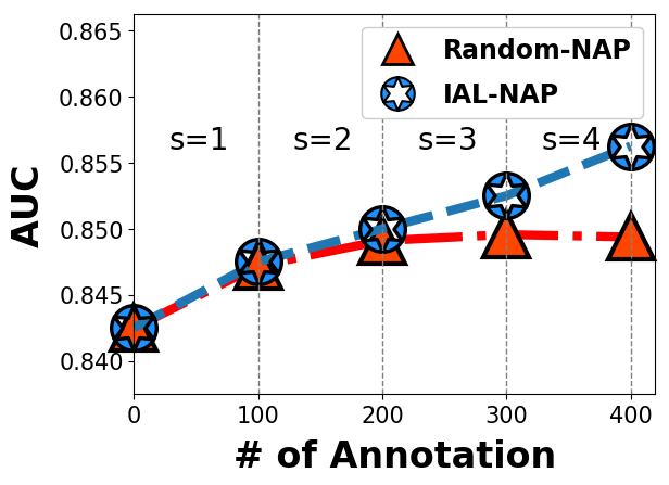
(c) CVD	(d) Squat

Figure 7: Change of accuracy with 100 annotations across four rounds ($S$) between IAL-NAP (blue) vs Random-NAP (red).

4 Experiments

4.1 Datasets and Baselines

1) Medical Check-ups

These datasets are subsets of the electronic health records (EHR) database of a major hospital, which consists of medical check-ups from $2009$ to $2012$ (4 timesteps) for patients over the age of 15 in out-patient units. We extracted $245,000$ patient records from the total of $1.5$ million records, each of which contains $34$ variables including general information (e.g., sex and height), vital signs (e.g., hemoglobin level), and risk-inducing behaviors (e.g., alcohol consumption). The task is to predict the onset of the following disease in the next year: 1) Heart Failure, 2) Cerebral Infarction, 3) Cardiovascular Disease (CVD).

2) Fitness - Squat Pose Correction

This dataset contains $4,000$ video frames of human subject performing squats, where the task is to predict whether the person is performing the squat with the correct posture or with one of ten different types of incorrect postures (e.g., 0: Correct posture, 1: Exaggerated knees-forward movement, 2: Sitting on the thighs). Thus this is a multi-label classification task. We extract 14 pairs of key points from joints (e.g., left shoulder or right ankle) over all frames, to clearly visualize which body joints an attention generator attends to for each instance.

3) Real Estate Sales Transactions

This datasets is a subset of public rolling sales transaction database (Zhu & Sobolevsky, 2018) from New York City Department of Finance that is publicly available, which consists of $70,700$ house records with $27,000$ sales transaction records over 10 years from 2010 to 2019 (10 time-steps). The subset used for experiments includes $3,100$ housing transactions, each of which includes 47 variables that describes the property (e.g. number of rooms), neighborhood (e.g. minimum distance to a supermarket), and macro-economy indicators (e.g., mortgage rate). The task is to make an one-year forecast for the price of a given residential property.

Baselines and our models
1) RETAIN: This is the attentional recurrent neural network model (RETAIN) proposed in (Choi et al., 2016).
2) Random-RETAIN: RETAIN, which is newly trained from a training set without $K$ randomly selected samples.
3) IF-RETAIN: RETAIN that is newly trained from the training set without the top $K$-negative points, which are obtained using the influence function (Koh & Liang, 2017).
4) Random-UA: This is the Uncertainty-Aware attentional network (UA) (Heo et al., 2018) which is trained using IAL with random instance and feature selection.
5) Random-NAP: Our IAL framework with Neural Attention Process model (NAP), which is trained using random instance and feature selection.
6) Cost-effective AILA: This is a modified version of the interactive attention learning model proposed by (Choi et al., 2019) which retrains the attention generator by using a binary cross entropy loss function between the attention vector $\bm{\alpha}_{k}$ and the attention annotation $\mathbf{m}_{k}$. We train the model with CER to verify the effectiveness of the NAP.
7) IAL-NAP Our IAL framework with Neural Attention Process (NAP) and cost-effective instance and feature Reranking (CER), which uses uncertainty for instance-wise reranking and counterfactual score for feature reranking.

Experimental setup For all datasets, we generate train/valid/test splits with the ratio of 70$\%$:10$\%$:20$\%$. For Random-UA and AILA model, we use $\ell_{2}$-regularization $\|\phi^{(s)}-\phi^{(s-1)}\|_{2}^{2}$ to prevent overfitting. Please see supplementary file for more details of the datasets, network configurations, and hyperparameters. We will also publicly release the codes and all datasets used in the experiments.

4.2 Experimental results

We first examine the prediction performance of the baselines and our models. Table 1 shows the results, where the performance is measured with Area Under the ROC curve (AUROC) on the risk prediction tasks, accuracy on squat posture task with multi-labels, and mean percentage error on real estate price forecasts. Note that IF-RETAIN, which uses influence functions to remove instances with negative influence scores, performs relatively better on most tasks than other RETAIN baselines, but fails to improve on CVD and squat posture task. We observe that Random-UA, which is retrained with human attention-level supervision on randomly selected samples, performs worse than Random-NAP on all tasks. This is due to overfitting to few supervised labels, while NAP does not suffer from overfitting. IAL-NAP significantly outperforms Random-NAP on all tasks, which shows that the effect of attention annotation cannot have much effect on the model when the instances are randomly selected. AILA with cost-effective reranking also performs worse than IAL-NAP, due to severe overfitting even with regularizations to prevent it. We further perform an ablation study of cost-effective reranking with different scoring measures in table 2. The results show that for instance-level scoring, influence and uncertainty scores work similarly, while the counterfactual score was the most effective for feature-wise reranking. However, considering the computation cost, the combination of uncertainty-counterfactual is the most cost-effective solution since it avoids expensive computation of the Hessians.

Effect of Neural Attention Process

Line plots in Figure 5 (top) shows averaged time to retrain examples over the rounds of interactions with Random-UA, AILA, Random-NAP, and IAL-NAP on the five tasks. IAL-NAP and Random-NAP shows shorter retraining time, while Random-UA and AILA which fine-tune the attention-generating network take a longer time to retrain. This shows another benefit of our neural attention process, which is its ability to perform amortized inference. A more responsive system can also improve the quality of the interaction, in the interactive learning setting.

Effect of Cost-Effective Re-ranking We further measure the average response time of the annotators with and without cost-effective reranking. Figure 5 (bottom) shows that annotators spend less time with annotation if variables are prioritized by their negative impacts measured using uncertainty (blue bars) compared to presenting them in the original order (grey bars), on all tasks. Figure 7 shows the change in model accuracy over training rounds with and without cost-effective reranking, where the negative impacts are measured by the influence score. On the risk prediction and squat posture tasks, the accuracy of IAL-NAP increases over the 4 rounds of interaction, while Random-NAP achieves only marginal increases. Especially, on the heart failure task (a), the line plot shows that IAL-NAP uses a smaller number of annotated examples (100 examples) than Random-NAP (400 examples) to improve the model with comparable accuracy (auc: 0.6414), which shows that IAL-NAP improves the model with fewer examples.

Qualitative analysis

We further analyze the contribution of each feature for a CVD patient (label=1) whose records showed significant changes in attention with the help of physicians in Figure 7. The table (top in Figure 7) shows the patient’s medical records at the previous (2009, 2010) and the current time-step (2011), yearly registered records. The three graphs shows the values of the allocated attentions across three rounds. Our model, IAL-NAP failed to predict the label at pretrained round (a), but makes a correct prediction at $s$=2 (c). We visualized five variables that have clinically meaningful changes. Across the change of attentions from (a) to (c), the physicians consider that attentions on age, HDL, and LDL in (a) are false positive (red bars) and smoking as false negative (blue bars), except SysBP as true positive (grey bars). Noting that the patient’s age (30) is younger than the median age (50 years-old) of female CVD patient (Garcia et al., 2016), initial IAL-NAP (a) allocated too much weights on age, which led to an overconfident attention model and in turn resulted in the incorrect prediction. However, our model gradually allocated less weights on age over rounds, as it started to learn what to attend to from interactive attention learning. Note that attention on smoking highly increased at $s$=2 (c), which is also clinically guided by a physician for the reason that CVD risk increases by 25$\%$ for women who smoke cigarettes (Huxley & Woodward, 2011). Previous incorrect attentions on HDL and LDL (a) decrease over rounds, since the HDL level (55 mg/dL) is in the normal range (40-60) and the level of LDL (102 mg/dL) is still lower than borderline high (130-159).

5 Conclusion

We proposed an interactive learning framework which iteratively learns by interacting with the human supervisors via the generated attentions. The framework utilizes a novel stochastic attention mechanism based on neural process that can correct the model’s interpretation from scarce human feedback without retraining or overfitting. Further, it uses cost-effective reranking of the instances and features by their negative impacts to maximize the effect of each human-machine interaction. We validated our model on five real-world tasks from the healthcare, real estate, and fitness domains, on which our model significantly outperforms baselines with smaller retraining and human annotation cost. Qualitative analysis of our model shows that it generates more human-interpretable attentions that is crucial for its reliability on safety-critical tasks.

Acknowledgements
This work was supported by Institute for Information $\&$ communications Technology Planning $\&$ Evaluation (IITP) grant funded by the Korea government (MSIT) (No.2017-0-01779, A machine learning and statistical inference framework for explainable artificial intelligence).

References

- Ahmad et al. (2018) Ahmad, M. A., Eckert, C., and Teredesai, A. Interpretable machine learning in healthcare. In Proceedings of the 2018 ACM International Conference on Bioinformatics, Computational Biology, and Health Informatics, pp. 559–560. ACM, 2018.
- Bahdanau et al. (2014) Bahdanau, D., Cho, K., and Bengio, Y. Neural machine translation by jointly learning to align and translate. arXiv preprint arXiv:1409.0473, 2014.
- Bahdanau et al. (2015) Bahdanau, D., Cho, K., and Bengio, Y. Neural machine translation by jointly learning to align and translate. ICLR, 2015.
- Bau et al. (2017) Bau, D., Zhou, B., Khosla, A., Oliva, A., and Torralba, A. Network dissection: Quantifying interpretability of deep visual representations. In Proceedings of the IEEE Conference on Computer Vision and Pattern Recognition, pp. 6541–6549, 2017.
- Bau et al. (2019) Bau, D., Zhu, J.-Y., Strobelt, H., Zhou, B., Tenenbaum, J. B., Freeman, W. T., and Torralba, A. Visualizing and understanding generative adversarial networks. arXiv preprint arXiv:1901.09887, 2019.
- Chi & Mu (2017) Chi, L. and Mu, Y. Deep steering: Learning end-to-end driving model from spatial and temporal visual cues. arXiv preprint arXiv:1708.03798, 2017.
- Choi et al. (2016) Choi, E., Bahadori, M. T., Sun, J., Kulas, J., Schuetz, A., and Stewart, W. Retain: An interpretable predictive model for healthcare using reverse time attention mechanism. In Advances in Neural Information Processing Systems, pp. 3504–3512, 2016.
- Choi et al. (2019) Choi, M., Park, C., Yang, S., Kim, Y., Choo, J., and Hong, S. R. Aila: Attentive interactive labeling assistant for document classification through attention-based deep neural networks. In Proceedings of the 2019 CHI Conference on Human Factors in Computing Systems, pp. 230. ACM, 2019.
- Clark et al. (2015) Clark, Ian, and Dumas, G. Toward a neural basis for peer-interaction: what makes peer-learning tick? Frontiers in psychology, 2015.
- Cook & Weisberg (1980) Cook, R. D. and Weisberg, S. Characterizations of an empirical influence function for detecting influential cases in regression. Technometrics, 22(4):495–508, 1980.
- Das et al. (2017) Das, A., Agrawal, H., Zitnick, L., Parikh, D., and Batra, D. Human attention in visual question answering: Do humans and deep networks look at the same regions? Computer Vision and Image Understanding, 163:90–100, 2017.
- Donahue & Grauman (2011) Donahue, J. and Grauman, K. Annotator rationales for visual recognition. In 2011 International Conference on Computer Vision, pp. 1395–1402. IEEE, 2011.
- Gal & Ghahramani (2016) Gal, Y. and Ghahramani, Z. Dropout as a bayesian approximation: Representing model uncertainty in deep learning. In ICML, 2016.
- Garcia et al. (2016) Garcia, M., Mulvagh, S. L., Bairey Merz, C. N., Buring, J. E., and Manson, J. E. Cardiovascular disease in women: clinical perspectives. Circulation research, 118(8):1273–1293, 2016.
- Garnelo et al. (2018) Garnelo, M., Schwarz, J., Rosenbaum, D., Viola, F., Rezende, D. J., Eslami, S. M. A., and Teh, Y. W. Neural processes. CoRR, abs/1807.01622, 2018. URL http://arxiv.org/abs/1807.01622.
- Gilpin et al. (2018) Gilpin, L. H., Bau, D., Yuan, B. Z., Bajwa, A., Specter, M., and Kagal, L. Explaining explanations: An overview of interpretability of machine learning. In 2018 IEEE 5th International Conference on Data Science and Advanced Analytics (DSAA), pp. 80–89. IEEE, 2018.
- Heo et al. (2018) Heo, J., Lee, H. B., Kim, S., Lee, J., Kim, K. J., Yang, E., and Hwang, S. J. Uncertainty-aware attention for reliable interpretation and prediction. In Advances in Neural Information Processing Systems, pp. 909–918, 2018.
- Hochreiter & Schmidhuber (1997) Hochreiter, S. and Schmidhuber, J. Long short term memory. Neural Computation, 9:1735–1780, 1997.
- Huxley & Woodward (2011) Huxley, R. R. and Woodward, M. Cigarette smoking as a risk factor for coronary heart disease in women compared with men: a systematic review and meta-analysis of prospective cohort studies. The Lancet, 378(9799):1297–1305, 2011.
- Ilyas et al. (2019) Ilyas, A., Santurkar, S., Tsipras, D., Engstrom, L., Tran, B., and Madry, A. Adversarial examples are not bugs, they are features. arXiv preprint arXiv:1905.02175, 2019.
- Koh & Liang (2017) Koh, P. W. and Liang, P. Understanding black-box predictions via influence functions. In Proceedings of the 34th International Conference on Machine Learning-Volume 70, pp. 1885–1894. JMLR. org, 2017.
- Lage et al. (2018) Lage, I., Ross, A., Gershman, S. J., Kim, B., and Doshi-Velez, F. Human-in-the-loop interpretability prior. In Advances in Neural Information Processing Systems, pp. 10159–10168, 2018.
- Ribeiro et al. (2016) Ribeiro, M. T., Singh, S., and Guestrin, C. "why should i trust you?": Explaining the predictions of any classifier. In Proceedings of the 22Nd ACM SIGKDD International Conference on Knowledge Discovery and Data Mining, KDD ’16, pp. 1135–1144, New York, NY, USA, 2016. ACM. ISBN 978-1-4503-4232-2. doi: 10.1145/2939672.2939778. URL http://doi.acm.org/10.1145/2939672.2939778.
- Salzberg (1994) Salzberg, S. L. C4. 5: Programs for machine learning by j. ross quinlan. morgan kaufmann publishers, inc., 1993. Machine Learning, 16(3):235–240, 1994.
- Sankar et al. (2019) Sankar, V., Kumar, D., Clausi, D. A., Taylor, G. W., and Wong, A. Sisc: End-to-end interpretable discovery radiomics-driven lung cancer prediction via stacked interpretable sequencing cells. arXiv preprint arXiv:1901.04641, 2019.
- Sato & Tsukimoto (2001) Sato, M. and Tsukimoto, H. Rule extraction from neural networks via decision tree induction. In IJCNN’01. International Joint Conference on Neural Networks. Proceedings (Cat. No. 01CH37222), volume 3, pp. 1870–1875. IEEE, 2001.
- Sener & Savarese (2017) Sener, O. and Savarese, S. Active learning for convolutional neural networks: A core-set approach. arXiv preprint arXiv:1708.00489, 2017.
- Sharif Razavian et al. (2014) Sharif Razavian, A., Azizpour, H., Sullivan, J., and Carlsson, S. Cnn features off-the-shelf: an astounding baseline for recognition. In Proceedings of the IEEE conference on computer vision and pattern recognition workshops, pp. 806–813, 2014.
- Tong (2001) Tong, S. Active learning: theory and applications, volume 1. Stanford University USA, 2001.
- Vaswani et al. (2017) Vaswani, A., Shazeer, N., Parmar, N., Uszkoreit, J., Jones, L., Gomez, A. N., Kaiser, Ł., and Polosukhin, I. Attention is all you need. In Advances in neural information processing systems, pp. 5998–6008, 2017.
- Xu et al. (2015) Xu, K., Ba, J. L., Kiros, R., Cho, K., Courville, A., Salakhutdinov, R., Zemel, R. S., and Bengio, Y. Show, attend and tell: Neural image caption generation with visual attention. In ICML, 2015.
- Yosinski et al. (2014) Yosinski, J., Clune, J., Bengio, Y., and Lipson, H. How transferable are features in deep neural networks? In Advances in neural information processing systems, pp. 3320–3328, 2014.
- Zaidan & Eisner (2008) Zaidan, O. and Eisner, J. Modeling annotators: A generative approach to learning from annotator rationales. In Proceedings of the 2008 conference on Empirical methods in natural language processing, pp. 31–40, 2008.
- Zhu & Sobolevsky (2018) Zhu, E. and Sobolevsky, S. House price modeling with digital census. arXiv preprint arXiv:1809.03834, 2018. URL https://www1.nyc.gov/site/finance/taxes/property-rolling-sales-data.page.