Secondary Electron Emission by
Plasmon Induced Symmetry Breaking in
Highly Oriented Pyrolitic Graphite (HOPG)

Abstract

Two-particle spectroscopy with correlated electron pairs is used to establish the causal link between the secondary electron spectrum, the $(\pi+\sigma)-$plasmon peak and the unoccupied band structure of highly oriented pyrolitic graphite. The plasmon spectrum is resolved with respect to the involved interband transitions and clearly exhibits final state effects, in particular due to the energy gap between the interlayer resonances along the $\Gamma$A-direction. The corresponding final state effects can also be identified in the secondary electron spectrum. Interpretation of the results is performed on the basis of density functional theory and tight binding calculations. Excitation of the plasmon perturbs the symmetry of the system and leads to hybridisation of the interlayer resonances with atom-like $\sigma^{*}$ bands along the $\Gamma A$-direction. These hybrid states have a high density of states as well as sufficient mobility along the graphite $c$-axis leading to the sharp $\sim$3 eV resonance in the spectrum of emitted secondary electrons reported throughout the literature.
PACS numbers: 68.49.Jk, 79.20.-m, 79.60.-i

Van der Waals materials have recently been attracting interest in materials science since they exhibit outstanding fundamental and technological properties and are building blocks for multilayered quasi 2D materials as well as 3D materials and heterostructures Geim and Grigorieva (2013); Novoselov and Castro Neto (2012). Graphite, being a model system for this class of materials has been most extensively studied with respect to its electronic structure, both experimentally Taft and Philip (1965); Willis et al. (1974); Klucker et al. (1974); Møller and Mohamed (1982); Papagno and Caputi (1983); Diebold et al. (1987); Maeda et al. (1988); Hoffman et al. (1990a); Strocov et al. (2000); Barrett et al. (2004a, b); Werner et al. (2015) and theoretically Wallace (1947); Slonczewski and Weiss (1958); Painter and Ellis (1970); Holzwarth* et al. (1982); Tatar and Rabii (1982); Marinopoulos et al. (2002).

When two or more graphene layers are put on top of each other, so-called interlayer resonances form in the electronic structure which are highly dispersive along the $c$-axis and reflect the three dimensional structure of the crystal Fauster et al. (1983). Distinct oscillations in the electron reflectivity are observed when measuring the reflected intensity as a function of the electron kinetic energy Hibino et al. (2008); Feenstra et al. (2013); Jobst et al. (2015), their number being equal to the number of graphene layers minus one. Interlayer states are highly transmissive for electrons coming from vacuum and have a large local density of states in between individual graphene layers. For graphite they appear as a broad band of states which strongly couple to vacuum Bellissimo et al. (2019). The character of such electronic multi-quantum well states can be qualitatively understood using the analogy to a Fabry-Pérot interferometer in light optics Geelen et al. (2019). The signal employed in the above techniques, such as elastic peak electron spectroscopy Geelen et al. (2019) and total current spectroscopy Strocov et al. (2000) exclusively stems from impinging electrons which are eventually detected without having suffered any energy loss, or are absorbed in their entirety, such as in inverse photoemission spectroscopy (IPES) experiments Fauster et al. (1983).

Compared to the works cited above, the present paper concerns the reverse process where electrons are leaving the surface after being liberated inside the solid. This phenomenon of secondary electron emission (SEE) is of great fundamental as well as technological importance Bellissimo et al. (2019). In the past, SEE has also extensively been employed to study the unoccupied electronic structure of graphite Willis et al. (1974); Klucker et al. (1974); Møller and Mohamed (1982); Papagno and Caputi (1983); Maeda et al. (1988); Hoffman et al. (1990a, b). Obviously, for secondary electron emission, energy losses, in particular excitation and decay of plasmons Eberlein et al. (2008); Shung (1986); Lin et al. (1997); Papageorgiou et al. (2000); Calliari et al. (2008, 2007); Guzzo et al. (2014) play an essential role. A striking difference between electronic structure data from SEE and the elastic techniques mentioned in the previous paragraph is that the dispersion of the interlayer resonances is not at all observed in SEE data. Instead, a strong resonance is found in secondary electron spectra which always appears at an energy of about 3 eV above vacuum (i.e. within the energy range of the first interlayer state above vacuum). The position of this resonance shows no dispersion whatsoever in SEE data and is found to be independent of the experimental kinematics in a substantial number of works by different authors Taft and Philip (1965); Willis et al. (1974); Klucker et al. (1974); Møller and Mohamed (1982); Papagno and Caputi (1983); Maeda et al. (1988); Hoffman et al. (1990a); Strocov et al. (2000).

We use time-correlated two-electron spectroscopy to establish a causal relationship between energy losses and secondary electron emission Voreades (1976); Scheinfein et al. (1993); Müllejans et al. (1993); Pijper and Kruit (1991); Werner et al. (2013) on a sample of highly oriented pyrolitic graphite (HOPG). In particular, secondary electron-electron energy loss coincidence spectroscopy (SE2ELCS) is employed (see supplemental information Werner et al. (2020)) to investigate the relationship between energy losses suffered by exciting a plasmon and the concomitant emission of a secondary electron. Note that for a given energy loss of the primary electron to be feasible, corresponding initial and final states need to exist in order to satisfy energy conservation. The electronic transitions taking place in resonance with the plasmon are explicitly identified experimentally. The experimental results highlight the influence of the complex band structure of HOPG on the plasmon spectrum and the ejection of a secondary electron in the course of the associated interband transition and are interpreted with the aid of density functional theory (DFT) and tight binding (TB) calculations Werner et al. (2020). In particular, when the symmetry of the system is broken in our tight binding model, the resulting hybridisation of the interlayer states with the atom-like $\sigma_{2}^{*}$-band leads to the $\sim$3 eV resonance in the SE spectrum.

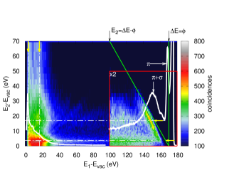
Figure 1: (color online) Double differential spectrum of true coincidences for HOPG for an incident energy of 173 eV above vacuum (energy resolution $\delta E_{1}=5$ eV). The white curve is the singles loss- and secondary electron spectrum. Indices ”1” and ”2” are used to indicate respectively fast and slow electrons arriving at detector 1, the hemispherical mirror analyser (HMA), and 2, the time of flight analyser (TOF) Werner et al. (2020). The green line labeled ”$E_{2}=\Delta E-\phi$” indicates the minimum energy loss needed for the slow liberated electron (”2”) to reach the vacuum level from the Fermi-level for a given energy loss $\Delta E$ where $\phi=4.6\ eV$ is the work function of HOPG. Here and below the yellow arrows correspond to final state energies of $E_{f}-E_{vac}=3.7$ eV and 17 eV, respectively.

Our experimental results are summarized in Figs. 1–3(a) showing different portions of the electron coincidence spectrum taken in specular reflection geometry at the Bragg maximum for a primary energy of $E_{0}-E_{vac}=173$ eV (see Ref Werner et al. (2020) for details). The white curve in Figs. 1 and 2(a) represents the singles electron spectrum, exhibiting the elastic peak, the $\pi-$ and $(\pi+\sigma)-$plasmon losses corresponding to minima in the real part of the dielectric function at $\hbar\omega_{\pi}\sim 6$ eV and $\hbar\omega_{\pi+\sigma}\sim 23$ eV Taft and Philip (1965). For higher energy losses plural plasmon excitation sets in. The secondary electron spectrum is characterized by a very sharp peak at 3.7 eV, which has been reported earlier by many authorsLaw et al. (1986); Caputi et al. (1986); Schafer et al. (1987); Willis et al. (1974); Møller and Mohamed (1982); Papagno and Caputi (1983); Maeda et al. (1988); Hoffman et al. (1990a, b); Strocov et al. (2000); Bellissimo et al. (2019) and a broad shoulder at $\sim$17 eV.

The coincidence spectrum shown in Fig. 1 represents the number of correlated electron pairs emitted for a given combination of energies ($E_{1},E_{2}$). When recording the spectrum of correlated electrons in a Bragg maximum, those processes dominate in which the primary electron is first deflected along the outgoing Bragg beam followed by the inelastic process. In the deflection-loss (DL) model, one thus assumes an initial momentum of the primary electron determined by the Bragg condition Diebold et al. (1987); Ruocco et al. (1999); Liscio et al. (2008a); Kheifets et al. (1998). As a consequence, all initial and final states of the inelastic process are fixed by momentum and energy conservation Werner et al. (2020); Liscio et al. (2008b). In other words, the coincidence experiment makes it possible to pinpoint the electronic transition of the bound electron involved in the (e,2e)-process by measuring time correlated electron pair intensities. In the present case this mainly concerns emission of a secondary electron after excitation and decay of a plasmon by the primary electron.

Three distinctly different parts can be identified in the coincidence spectrum: (1) a region of high intensity near the green line labeled $E_{2}=\Delta E-\phi$. Comparison with the singles spectrum allows one to conclude that this feature corresponds to the excitation of a single plasmon, which is shown separately in Fig. 2(a); (2) horizontal stripes along the $E_{1}$-scale at energies $E_{2}=$3.7 and 17 eV, indicated by the yellow arrows, which seem to have a counterpart along the $E_{2}$ scale (vertical dashed lines marked by yellow arrows). This energy region will be referred to as the plural scattering region in the following; and (3) a strong and structured peak for energies $E_{1},E_{2}\leq 20$ eV, corresponding to the cascade of secondary electrons. A distinct peak of what appears to be correlated electron emission is seen around the point ($E_{1},E_{2})=(17,17)$ eV.

Fig. 2(b) shows the region in phase-space corresponding to the plasmon loss in Fig. 2(a), obtained by applying energy and momentum conservation (See Eqns. 1-3 of Werner et al. (2020)) to the data within the red parallelogram in Fig. 2(a). The colored arrows in Fig. 2(b) indicate the interband transitions corresponding to the energies of the fast and slow electrons marked by colored dots in Fig. 2(a).

Finally, in Fig. 3 the total electron yield (TEY) measured in absolute units (green curve, Bellissimo et al. (2019)) is compared with the coincidence data in Fig. 1 summed over $E_{1}$ (blue curve) and the singles SE spectrum (black curve). The lower panel compares the band structure along the $\Gamma$A-direction with the DFT-results for the symmetry conserved (purple) and symmetry broken (red) case.

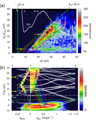
Figure 2: (color online) (a). Coincidence spectrum of the plasmon loss in HOPG (measured with an energy resolution $\delta E_{1}=1.25$ eV.) The white curve is the singles loss spectrum. (b) The data in the plasmon feature in (a) within the red parallelogram represented in $k$-space and projected on the pertinent band structure Riccardi (2019) along the $\Gamma A$- and $\Gamma K$-direction (see supplemental material). The colored arrows in the panels labeled $\Gamma$A and $\Gamma$K are projections of the initial and final states on these crystallographic directions corresponding to the colored dots in (a).

A striking feature of the single scattering plasmon feature is the complete absence of the $\pi$-plasmon in the coincidence data, in particular also at low energies: finite count rates appear only for $\Delta>$12 eV. This can be understood on the basis of the $k$-space representation of the data in Fig. 2(b): for the characteristic energy loss of the $\pi$-plasmon and the kinematics of the experiment, no favorable combination of initial and final states above vacuum is available which would allow a transition to take place Bellissimo et al. (2019). Note that our experiment mainly samples around $q_{\parallel}\sim 0.5\rm{\AA}^{-1}$, exhibiting an energy gap between valence and conduction band.

The coincidence data also convey the fact that plural inelastic scattering proceeds via a Markov-type process Werner et al. (2011); Bellissimo et al. (2019), i.e. no memory of the previous collision plays a role in subsequent processes. If this were not the case, i.e. if coherent plural plasmon creation took place in which the full energy loss is transferred to a single electron, intensity due to plasmon replicas should appear just below the green diagonal line at energies $(E_{1},E_{2})=(E_{0}-n\times\hbar\omega_{\pi+\sigma},n\times\hbar\omega_{\pi+\sigma}-\phi+E_{b})$. Here $n$ is an integer and $E_{b}$ is the (negative) binding energy of the initial state. Likewise, no plasmon replicas are seen for ejected electron energies corresponding to a single plasmon loss, i.e. at energies near $(E_{1},E_{2})=(E_{0}-n\times\hbar\omega_{\pi+\sigma},\hbar\omega_{\pi+\sigma}-\phi+E_{b})$. Instead, stripes of intensity at energies (marked by the yellow arrows) of 3.7 and 17 eV, respectively are observed. The fact that the ejected electron energy in the plural scattering region is completely independent of $\Delta E$ cannot be understood within the DL-model. The explanation is that when more than one inelastic process occurs, any combination of scattering angles and energy losses in individual scattering events can lead to the net energy and momentum transfer observed for the ejected electron. In other words, the initial state for the process leading to ejection of the second electron is no longer determined as in the single scattering feature (see Fig. 2(a)). This implies that the DL-model is only valid in the single scattering regime. The final state in the plural scattering regime, however, is determined by the detection geometry and energy of the slow electron. Indeed, the energies at which these stripes appear seem to correspond to the position of the atom-like $\sigma_{2}^{*}$-bands, as well as the flat $\sigma^{*}$-bands 22 eV above Fermi, along the $\Gamma A$-direction (see Fig. 3). Note that the $\Gamma A$-direction coincides with the symmetry axis of the TOF analyser, which measures the final state of the slow electron.

For any energy loss $\Delta E$ in the single scattering plasmon feature the probability for generating a secondary electron has a strong peak at energies $E_{2}$ within the plasmon feature. This observation highlights the fact that the final state of the scattering process corresponds to the ejection of a single bound electron. Any conceivable process in which the energy is transferred to more than one electron in the final state would lead to intensity below the single scattering plasmon feature for any reasonable energy sharing model. Furthermore, the intensity in the single scattering feature is seen to occur for a range of slightly different binding energies (energetic distance from the green diagonal) when going from top to bottom, following the dispersion of the initial state. This is indeed confirmed by the representation of the single scattering data in $k$-space, Fig. 2(b). A faint minimum is seen in the plasmon loss feature in Fig. (1) near $(E_{1},E_{2})=(154,10)$ eV, corresponding to the energy gap in between the strongly dispersing interlayer bands along $\Gamma A$ indicated by the yellow arrows in Fig. 2(b). Indeed, a minimum in the final state intensity is also observed in the plasmon spectrum in Fig. 2(b) at $E-E_{F}\sim$15 eV.

These findings show that for a material with a complex band structure, such as graphite, the excitation of a plasmon and the associated interband transitions are both essential parts of the same coherent process, a plasmon-assisted interband transition Kouzakov and Berakdar (2012) leading to ejection of the bound electron into an excited state. This picture supports the momentum-exciton model for the plasmon Ferrell and J. (1958); Bellissimo et al. (2019) as a coherent excitation of a (rather small) number of electron hole pairs behaving as a quasi-particle with a well-defined energy and momentum. Note that the typical number of electrons participating in a plasmon is about five Ferrell and J. (1958); Egri (1983) and that the range of possible energies above vacuum occupied by the ejected electron is limited by the plasmon energy. This implies that the width of the secondary electron peak is essentially governed by the density of the solid state electrons.

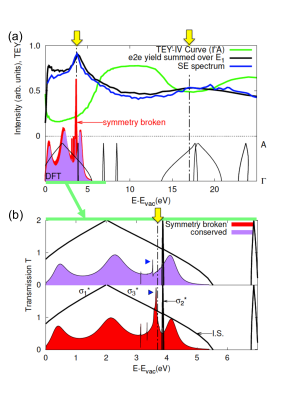
Figure 3: (color online) (a) Green curve: total electron yield (TEY) measured in absolute units Bellissimo et al. (2019); Blue curve: coincidence data in Fig. 1 summed over $E_{1}$; black curve: singles SE spectrum (white curve in Fig. 1). The lower panel compares the band structure along $\Gamma$A with the DFT-results for the symmetry conserved (purple) and symmetry broken (red) case. (b) Theoretical total transmission of graphite surface as a function of initial energy for symmetry-conserved (upper panel) and symmetry-broken (lower panel) slab. Blue triangles mark the transmission peak caused by the $\sigma_{2}^{*}$ band. In the symmetry-conserved slab, this resonance is very sharp, containing few electrons, while it becomes much more pronounced in the symmetry-broken slab due to hybridisation (see text).

Finally, the energies of the secondary electrons emitted along the graphite $c$-axis (stripes in the plural scattering region marked with yellow arrows) and the sharp peak in the SE spectrum at 3.7 eV exhibiting a surprising lack of dispersion Law et al. (1986); Caputi et al. (1986); Schafer et al. (1987); Willis et al. (1974); Møller and Mohamed (1982); Papagno and Caputi (1983); Maeda et al. (1988); Hoffman et al. (1990a, b); Strocov et al. (2000); Bellissimo et al. (2019) deserve to be discussed. These features appear energetically very close to the flat $\sigma_{2}^{*}$- bands within the interlayer resonances along $\Gamma A$ (Fig.2(b)). To understand their origin we use DFT calculations for bulk graphite as well as a surface slab to parameterize a tight binding model Linhart et al. (2019). We can then simulate the transmission of the secondary electron from a Bloch state inside the solid, i.e. the final state of the inelastic scattering process with the incoming electron to a free vacuum state (as given by Eq. (6) in the supplemental material). Given an unperturbed graphite slab, we find, as expected by the flat nature of the $\sigma_{2}^{*}$ bands, a very sharp resonance (see blue triangle in upper panel of Fig. 3(b)) that does not contribute significantly to the overall signal, as its area is vanishingly small. We next aim to model the symmetry breaking induced by the incidence of the primary electron and the emerging plasmon in the simplest way possible: we induce a symmetry-breaking at the surface of the slab by a local potential $V_{\delta\mathrm{sp^{2}}}\approx 0.3eV$ added to a single of the three equivalent $\mathrm{sp}^{2}$ orbitals of each carbon atom of the surface layer. Such a term breaks the $D_{6h}$ symmetry of graphite, essentially locally eliminating the three-fold symmetry. The induced hybridisation between the $\sigma_{2}^{*}$ bands and $\sigma_{1,3}^{*}$-interlayer bands substantially enhances and broadens the resonance. The resulting hybrid state exhibits the high density of states of the flat band, implying that it is a favorable state for an initially bound electron to reach a final state above the vacuum level. The hybrid state also has the high mobility of the interlayer state which efficiently couples to vacuum, allowing it to escape from the surface. We have verified numerically that a similar symmetry breaking in bulk HOPG leads to transmission from $\sigma_{2}^{*}$ to $\sigma_{1,3}^{*}$ modes (and vice versa) in bulk transport perpendicular to the layers.

Since the parametrization of our tight-binding model only extends to about 18 eV, the origin of the second stripe in the coincidence data at $E-E_{F}\sim$17 eV could not be verified. It is conjectured however, that a similar hybridisation mechanism plays a role in that case as for the lower lying interlayer band around 3.7 eV. The peak of apparent correlated emission at $(E_{1},E_{2})=(17,17)$ eV then is a direct consequence of the hybridisation in that also the unoccupied flat band at around 17 eV (above vacuum) is a favorable final state and by virtue of the high mobility of the hybridized state also leads to a strong peak in the secondary electron cascade. For the primary energy $E_{0}=$173 eV employed here, plural inelastic processes can lead to (incoherent) creation of several secondary electrons. A part of these SEs may actually escape and give rise to multi-electron detection events with prefered energies of 17 eV. As discussed above, this proceeds via a Markov sequence of events leading to a strong preference of final states with these energies in the course of (incoherent) plural inelastic scattering and generation of secondary electrons. Therefore, while the peak at $(E_{1},E_{2})=(17,17)$ eV appears to be due to correlated electron emission, it rather is an incoherent increase in the electron pair intensity due to the aforementioned process. A similar peak is also expected at $(E_{1},E_{2})=(3.7,3.7)$ but could not be observed since the lowest energy along the $E_{1}$-scale that can be reached in the coincidence experiment is $\sim$10 eV.

In summary, the $(\pi+\sigma)$-plasmon in graphite has been resolved with respect to the involved electronic transitions. Formation of a hybrid state as a consequence of plasmon induced symmetry breaking provides an explanation for the strong resonance observed in SE-spectra in the literature (at 3.7 eV in the present work). Most importantly, it explains the difference in band structure measurements using elastic processes and techniques which involve creation of plasmon. To fully appreciate this point the reader is referred to Fig. 4 in Ref. Maeda et al. (1988) which shows a direct comparison of IPES and SEE data, the dispersion of the interlayer state completely lacking in the latter. The results therefore indicate that the inverse-LEED (Low Energy Electron Diffraction) formalism which is often employed to interpret secondary electron spectra Lüth (2010) should be complemented to account for many body processes, since the phenomenon of secondary electron emission cannot be fully described on the basis of the one-electron band structure.

Acknowledgments
The authors express their gratitude to P. Riccardi and E. Krasovskii for fruitful discussions and P. Riccardi for providing detailed band structure data of graphite. Financial support by the FP7 People: Marie-Curie Actions Initial Training Network (ITN) SIMDALEE2 (Grant No. PITN 606988) is gratefully acknowledged. FL and LL acknowledge support by FWF program I 3827-N36. The computational results presented have been achieved using the Vienna Scientific Cluster (VSC).

.

Supplemental Material for ”Secondary Electron Emission by
Plasmon Induced Symmetry Breaking in
Highly Oriented Pyrolitic Graphite (HOPG)”
Wolfgang S.M. Werner, Vytautas Astašauskas,

Philipp Ziegler, Alessandra Bellissimo,
Giovanni Stefani, Lukas Linhart
and Florian Libisch.

I Experimental

The sample was a HOPG crystal of ZYB quality with a nominal mosaic spread of $(0.8\pm 0.2)^{\circ}$, mechanically exfoliated in air and annealed for several hours at 500^∘C in the UHV system with a base pressure of 2$\times 10^{-10}$ mbar housing the spectrometer. During the measurement, the pressure rises to 5$\times 10^{-10}$ mbar.

The employed coincidence spectrometer is schematically shown in Fig. 4. Arrival-time differences of electron pairs are recorded for a hemispherical mirror analyser (HMA, measuring the fast scattered electron, subscript ’1’), and a time of flight analyser (TOF, measuring the slow ejected electron, subscript ’2’). While the HMA has a constant energy resolution $\delta E_{1}$ (equal to 5 eV and 1.25 eV for the data presented in Fig. 1 and Fig. 2 respectively), the energy resolution of the TOF-analyser is about $\delta E_{2}=1$ eV at an energy of 20 eV, while it is several tens of an eV at an energy of 200 eV. The white curve in Fig. 1 representing the singles energy loss and SE spectrum was measured with the HMA with a pass energy of 5 eV corresponding to an energy resolution of $\delta E_{1}=0.25$ eV. The lowest energy which can be recorded by the HMA depends on the employed pass energy and is equal to 10 eV for the coincidence data in Fig. 1, while it is 0.5 eV for the singles spectrum (white curve). Coincidence spectra were measured at a primary energy $E_{0}-E_{vac}=173$ eV, corresponding to a Bragg maximum for this geometry, after carefully aligning the sample in the specular reflection geometry, by directing the Bragg beam into the central angle of the HMA.

The coincidence spectra are obtained with a continuous electron beam in order to increase the effective coincidence rate. Flight times for each energy measured by the hemispherical analyser are measured before the coincidence measurement using a pulsed electron beam. In this way, the flight time of an electron in a correlated pair reaching the time of flight detector during the coincidence measurement is calibrated. Coincident flight time spectra for each energy measured with the HMA are superimposed on a flat background of false coincidences which is subtracted, leading to the spectra of true coincidences as shown in Fig. 1 and Fig. 2. The current incident on the sample during the coincidence measurement amounted to 70 fA, obtained by comparing elastic peak intensities with picoamperemeter results down to the nA range. In this way, the spectrometer transmission and other experimental factors are calibrated giving absolute values at any lower current using the elastic peak intensity. The acquisition time for the coincidence data shown in Fig. 1 as well as for the coincidence data in Fig. 2 amounted to approximately 14 days.

Note that both analysers are located in the scattering plane. The opening angles of the analysers amount to $\Delta\Omega_{HMA}=10^{\circ}$ and $\Delta\Omega_{TOF}=12^{\circ}$. Owing to the employed experimental geometry (see Fig. 4), the axis of the TOF analyser is aligned with the $\Gamma A$ crystallographic direction (i.e. the $c$-axis in graphite), while the HMA intensity consists of components along the $\Gamma A$ as well as the $\Gamma K$ and $\Gamma M$-crystallographic direction. Due to the wide opening angle of the hemispherical analyser the momenta sampled in the occupied band structure extend to about 1$\rm{\AA}^{-1}$. Since the $\Gamma M$ and $\Gamma K$ band structure are similar to each other near the $\Gamma$-point and cannot be distinguished within our experimental energy and angular resolution we only present and discuss the $\Gamma K$-portion in the text for clarity. While for the occupied states, the $q_{\parallel},q_{\perp}$-region sampled in phase space is mainly governed by the angular acceptance of the HMA, the acceptance of the TOF governs the portion of final state phase space, which becomes particularly narrow for the $\Gamma A$-direction owing to the increase of $k_{\perp}$ inside the solid (see below).

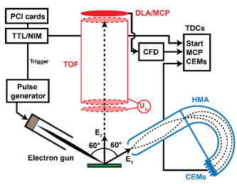
Figure 4: (color online) Schematic illustration of the experimental setup. (see text).

II Data interpretation

In the specular reflection geometry, diffraction of the incoming beam by the graphene planes gives rise to a Bragg beam oriented exactly along the specular direction inside the solid, which then can induce an inelastic process. In the UV-energy range an energy loss is predominantly accompanied by an electronic transition, which leads to liberation of a second electron inside the solid. For sufficiently large losses, this electron may overcome the surface potential barrier and is ejected from the surface. This deflection-loss (DL) model Diebold et al. (1987); Ruocco et al. (1999); Liscio et al. (2008a); Kheifets et al. (1998) implies that the scattering kinematics of the inelastic collision are fully determined. In other words, under such conditions, the final state of the correlated electron pair in an (e,2e) experiment is fixed by the energy and direction of detection and together with the known state of the primary electron, the initial state of the ejected solid state electron is fully determined. Here we designate the scattered and ejected electron by the indices ”s” and ”e”, while in the main text we merely distinguish between events where electrons are detected in analyser 1 and 2 and label the energy scales accordingly. This is strictly speaking correct and necessary because of the indistinguishability of electrons but generally identifying electron 1 with the scattered (fast) electron and electron 2 with the ejected (slow) electron will be correct in many cases. The binding energy $E_{b}(\vec{q})$ of the bound electron is found by requiring that the energy loss of the primary electron $\Delta E=E_{0}-E_{s}$ –where the index ”0” indicates the primary electron– is used to liberate the bound electron from the solid, by overcoming the work function $\Phi$, and that it is ultimately ejected from the solid with an energy $E_{e}$:

$$\Delta E=E_{0}-E_{s}=E_{e}+\Phi-E_{b}(\vec{q}),$$ (1)

where the binding energy is counted from the Fermi level and is negative. Momentum conservation yields for the momentum of the bound electron:

$$\vec{q}=\vec{k}_{e}-(\vec{k}_{0}-\vec{k}_{s})+\vec{G}=\vec{k}_{e}-\Delta\vec{K}+\vec{G},$$ (2)

where $\vec{G}$ is a reciprocal lattice vector and $\Delta\vec{K}$ is the momentum transfer. The above equation holds inside the solid. To convert the momenta inside the solid to the momenta measured in vacuum (or vice versa), the increase of the energy by the inner potential $U_{i}$ when the electron crosses the surface potential barrier needs to be accounted for. Using atomic units ($\hbar=m_{e}=e=1$) the relationship between the perpendicular component of momentum inside and outside the solid can be expressed as follows:

$$\frac{k^{2}_{\perp,in}}{2}=\frac{k^{2}_{\perp,out}}{2}+U_{i},$$ (3)

while the parallel momentum is conserved as the electron penetrates the barrier.

The inner potential $U_{i}$ has been determined by measuring the elastic peak intensity as a function of the vacuum energy $E_{v}$ and identifying the $n$-th order Bragg maximum $E_{Bragg}(n)$. Using the Equation Ruocco et al. (1999):

$$E_{Bragg}(n)=\Big{\{}\frac{n^{2}\pi^{2}}{2d^{2}}-U_{i}\Big{\}}\frac{1}{\cos^{2}\alpha},$$ (4)

which is written here in atomic units with $d$ the interlayer distance and $\alpha$ the vacuum polar angle of incidence and emission, we have plotted the Bragg energies in vacuum against $n^{2}$ and determined the inner potential from the axis offset after fitting the data to a straight line. The value of $U_{i}=16.1~{}eV$ obtained in this way is in good agreement with values found in the literature (see Ref. Ruocco et al. (1999) and references therein).

Using Eqns. 1–3, values of the initial and final state energies and momenta are determined for each pixel in the data of Fig. 2(a). The corresponding intensity in each pixel is added to a histogram in $k$-space, eventually leading to the results shown in Fig. 2(b). The portion of phase space along the $\Gamma$A-direction becomes very narrow due to the significant increase of the perpendicular momentum component when the electron feels the inner potential of $U_{i}=16.1$ eV.

III Theory

Given the complexity of the inelastic scattering processes inside HOPG, we do not model this process beyond the energy and momentum conservation considerations outlined above. Instead, we aim to elucidate the ejection process of the ejected electron by considering its scattering from an initial state inside the HOPG target (the final state of the inelastic scattering process) to a final propagating state outside of the solid (resulting in a signal at the detector). We first model bulk graphite and a graphite surface slab using density functional theory (DFT) employing the VASP software package Kresse and Furthmüller (1996). We then use a Wannier localization procedureMarzari and Vanderbilt (1997); Souza et al. (2001) to obtain local tight-binding parameters for the bulk and the surface slab following Linhart et al. (2019). We verify that our tight binding model reproduces the full DFT single-particle band structure. Since we are interested in electron emission at higher energies, we take great care in obtaining a converged band structure at energies up to 20 eV in VASP using appropriate convergence thresholds. Given the strong entanglement of higher-lying virtual bands, our tight binding model only correctly reproduces bands up to 18 eV.

Using our Wannier representation, we compose a tight-binding Hamiltonian $H$ containing a large number of bulk layers, four surface layers from the slab and free electron states outside the slab. We obtain a scattering problem by introducing open boundary conditions at both sides by infinite waveguides representing graphite Bloch states (incoming lead) and free particle states (outgoing lead). The Green’s function of this system is given by

$$G(E)=\left[H-E-\Sigma_{Gr}(E)-\Sigma_{V}(E)\right]^{-1},$$ (5)

where the self-energies $\Sigma_{Gr}$ ($\Sigma_{V}$) represent the open boundary conditions of bulk graphite (vacuum). We solve the scattering problem using our modular recursive Green’s function approach Libisch et al. (2012) to determine the probability $T(\mathbf{k}_{B})$ of an electron in an initial Bloch state $\mathbf{k}_{B}$ with energy $\varepsilon_{\mathbf{k}_{B}}$ inside the solid transfering to a propagating vacuum state,

$$T(\mathbf{k}_{B})=\int_{D}d\mathbf{k}_{v}\left|\left<\phi_{\mathbf{k}_{B}}\right|G(\varepsilon_{\mathbf{k}_{B}})\left|\mathbf{k}_{v}\right>\right|^{2}\delta(\varepsilon_{\mathbf{k}_{B}}-\mathbf{k}_{v}^{2}/2m)$$ (6)

where the integral over the vacuum wave vector $\mathbf{k}_{v}$ goes over those final states that can reach the detector in the experimental setup, and the delta function ensures energy conservation.

References

- Geim and Grigorieva (2013) A. K. Geim and I. V. Grigorieva, Nature 499, 419 (2013), ISSN 00280836, eprint 1307.6718, URL http://dx.doi.org/10.1038/nature12385.
- Novoselov and Castro Neto (2012) K. S. Novoselov and A. H. Castro Neto, Physica Scripta T146 (2012), ISSN 00318949.
- Taft and Philip (1965) E. A. Taft and H. R. Philip, Phys. Rev. 138 (1965).
- Willis et al. (1974) R. F. Willis, B. Fitton, and G. S. Painter, Physical Review B 9, 1926 (1974), ISSN 01631829.
- Klucker et al. (1974) R. Klucker, M. Skibowski, and W. Steinmann, Phys stat sol (b) 65, 703 (1974).
- Møller and Mohamed (1982) P. J. Møller and M. H. Mohamed, JPC 15, 6457 (1982).
- Papagno and Caputi (1983) L. Papagno and L. S. Caputi, Surface Science 125, 530 (1983), ISSN 00396028.
- Diebold et al. (1987) U. Diebold, A.Preisinger, P.Schattschneider, and P.Varga, SS 197, 430 (1987).
- Maeda et al. (1988) F. Maeda, T. Takahashi, H. Ohsawa, S. Suzuki, and H. Suematsu, Physical Review B - Condensed Matter and Materials Physics 37, 4482 (1988).
- Hoffman et al. (1990a) A. Hoffman, G. L. Nyberg, and S. Prawer, Journal of Physics: Condensed Matter 2, 8099 (1990a), ISSN 09538984.
- Strocov et al. (2000) V. Strocov, P. Blaha, H. Starnberg, M. Rohlfing, R. Claessen, J.-M. Debever, and J.-M. Themlin, Phys. Rev. B 61, 4994 (2000).
- Barrett et al. (2004a) N. Barrett, E. E. Krasovskii, J. M. Themlin, and V. N. Strocov, Surface Science 566-568, 532 (2004a), ISSN 00396028.
- Barrett et al. (2004b) N. Barrett, E. E. Krasovskii, J. M. Themlin, and V. N. Strocov, Surface Science 566-568, 532 (2004b), ISSN 00396028.
- Werner et al. (2015) W. S. M. Werner, A. Bellissimo, R. Leber, A. Ashraf, and S. Segui, Surface Science 635, L1 (2015).
- Wallace (1947) P. Wallace, Phys. Rev. 71, 622 (1947).
- Slonczewski and Weiss (1958) J. C. Slonczewski and P. R. Weiss, Physical Review 169, 272 (1958).
- Painter and Ellis (1970) G. S. Painter and D. E. Ellis, Physical Review B 1, 4747 (1970), ISSN 01631829.
- Holzwarth* et al. (1982) N. A. W. Holzwarth*, S. G. Louie, and S. Rabii, Phys. Rev. B 5382 (1982).
- Tatar and Rabii (1982) R. C. Tatar and S. Rabii, Phys. Rev. B 25, 4126 (1982), URL https://link.aps.org/doi/10.1103/PhysRevB.25.4126.
- Marinopoulos et al. (2002) A. G. Marinopoulos, L. Reining, V. Olevano, A. Rubio, T. Pichler, X. Liu, M. Knupfer, and J. Fink, Physical Review Letters 89, 1 (2002), ISSN 10797114.
- Fauster et al. (1983) T. Fauster, F. J. Himpsel, J. E. Fischer, and E. W. Plummer, Physical Review Letters 51, 430 (1983), ISSN 00319007.
- Hibino et al. (2008) H. Hibino, H. Kageshima, F. Maeda, M. Nagase, Y. Kobayashi, and H. Yamaguchi, Physical Review B - Condensed Matter and Materials Physics 77, 1 (2008), ISSN 10980121, eprint 0710.0469.
- Feenstra et al. (2013) R. M. Feenstra, N. Srivastava, Q. Gao, M. Widom, B. Diaconescu, T. Ohta, G. L. Kellogg, J. T. Robinson, and I. V. Vlassiouk, Physical Review B - Condensed Matter and Materials Physics 87, 1 (2013), ISSN 10980121, eprint 1211.6676.
- Jobst et al. (2015) J. Jobst, J. Kautz, D. Geelen, R. M. Tromp, and S. J. Van Der Molen, Nature Communications 6, 1 (2015), ISSN 20411723.
- Bellissimo et al. (2019) A. Bellissimo, P. Gian-Marco, A. Ruocco, G. Stefani, O. Ridzel, V. Astašauskas, M. Taborelli, and W. S. Werner (2019).
- Geelen et al. (2019) D. Geelen, J. Jobst, E. E. Krasovskii, S. J. van der Molen, and R. M. Tromp, Physical Review Letters 123, 86802 (2019), ISSN 1079-7114, eprint 1904.13152, URL http://arxiv.org/abs/1904.13152.
- Hoffman et al. (1990b) A. Hoffman, G. L. Nyberg, and S. Prawer, Journal of Physics: Condensed Matter 2, 8099 (1990b), ISSN 09538984.
- Eberlein et al. (2008) T. Eberlein, U. Bangert, R. R. Nair, R. Jones, M. Gass, A. L. Bleloch, K. S. Novoselov, A. Geim, and P. R. Briddon, Physical Review B - Condensed Matter and Materials Physics 77, 1 (2008), ISSN 10980121.
- Shung (1986) K. W. Shung, Phys. Rev. B34, 979 (1986).
- Lin et al. (1997) M. Lin, C. Huang, and D. Chuu, Physical Review B - Condensed Matter and Materials Physics 55, 13961 (1997), ISSN 1550235X.
- Papageorgiou et al. (2000) N. Papageorgiou, M. Portail, and J. M. Layet, Surface Science 454, 462 (2000), ISSN 00396028.
- Calliari et al. (2008) L. Calliari, S. Fanchenko, and M. Filippi, Surface and Interface Analysis 40, 814 (2008), ISSN 01422421.
- Calliari et al. (2007) L. Calliari, S. Fanchenko, and M. Filippi, Carbon 45, 1410 (2007), ISSN 00086223.
- Guzzo et al. (2014) M. Guzzo, J. J. Kas, L. Sponza, C. Giorgetti, F. Sottile, D. Pierucci, M. G. Silly, F. Sirotti, J. J. Rehr, and L. Reining, Physical Review B - Condensed Matter and Materials Physics 89, 1 (2014), ISSN 10980121.
- Voreades (1976) D. Voreades, Surf. Sci. 60, 325 (1976).
- Scheinfein et al. (1993) M. R. Scheinfein, J. Drucker, J. Liu, and J. K. Weiss, Phys. Rev. B47, 4069 (1993).
- Müllejans et al. (1993) H. Müllejans, A. L. Bleloch, A. Howie, and M. Tomita, Ultramicroscopy 52, 360 (1993).
- Pijper and Kruit (1991) F. J. Pijper and P. Kruit, Phys. Rev. 44, 9192 (1991).
- Werner et al. (2013) W. S. M. Werner, F. Salvat-Pujol, A. Bellissimo, R. Khalid, W. Smekal, M. Novak, A. Ruocco, and G. Stefani, Phys. Rev. B88, 201407 (2013).
- Werner et al. (2020) W. S. M. Werner, V. Astašauskas, P. Ziegler, A. Bellissimo, L. Linhart, and F. Libisch, Phys. Rev. Lett. pp. This work, supplemental material (2020).
- Law et al. (1986) A. R. Law, M. T. Johnson, and H. P. Hughes, Physical Review B 34, 4289 (1986), ISSN 01631829.
- Caputi et al. (1986) L. S. Caputi, G. Chiarello, A. Santaniello, E. Colavita, and L. Papagno, Phys Rev B 34, 6080 (1986).
- Schafer et al. (1987) I. Schafer, M. Schlüter, and M. Skibowski, Phys Rev B 35 (1987).
- Ruocco et al. (1999) A. Ruocco, M. Milani, S. Nannarone, and G. Stefani, Phys. Rev. B 59, 13359 (1999).
- Liscio et al. (2008a) A. Liscio, A. Ruocco, G. Stefani, and S. Iacobucci, Phys. Rev. B 77, 085116 (2008a).
- Kheifets et al. (1998) A. S. Kheifets, S. Iacobucci, A. Ruocco, R. Camilloni, and G. Stefani, Phys. Rev. B 57 (1998).
- Liscio et al. (2008b) A. Liscio, A. Ruocco, G. Stefani, and S. Iacobucci, Phys. Rev. B 77 (2008b).
- Riccardi (2019) P. Riccardi, priv.comm. (2019).
- Werner et al. (2011) W. S. M. Werner, F. Salvat-Pujol, W. Smekal, R. Khalid, F. Aumayr, H. Störi, A. Ruocco, F. Offi, G. Stefani, and S. Iacobucci, Appl. Phys. Lett. 99, 184102 (2011).
- Kouzakov and Berakdar (2012) K. A. Kouzakov and J. Berakdar, Phys. Rev. A85, 022901 (2012).
- Ferrell and J. (1958) R. A. Ferrell and Q. J. J., Physical Review 109, 653 (1958), ISSN 0031899X.
- Egri (1983) I. Egri, Z. Phys. B53, 183 (1983).
- Linhart et al. (2019) L. Linhart, M. Paur, V. Smejkal, J. Burgdörfer, T. Mueller, and F. Libisch, Phys. Rev. Lett. 123, 146401 (2019), URL https://link.aps.org/doi/10.1103/PhysRevLett.123.146401.
- Lüth (2010) H. Lüth, Solid Surfaces, Interfaces and Thin Films (2010), sixth ed., ISBN 978–3–319–10756–1.
- Kresse and Furthmüller (1996) G. Kresse and J. Furthmüller, Computational Materials Science 6, 15 (1996), URL https://doi.org/10.1016/0927-0256(96)00008-0.
- Marzari and Vanderbilt (1997) N. Marzari and D. Vanderbilt, Physical Review B 56, 12847 (1997), URL https://doi.org/10.1103/physrevb.56.12847.
- Souza et al. (2001) I. Souza, N. Marzari, and D. Vanderbilt, Physical Review B 65 (2001), URL https://doi.org/10.1103/physrevb.65.035109.
- Libisch et al. (2012) F. Libisch, S. Rotter, and J. Burgd rfer, New Journal of Physics 14, 123006 (2012), URL https://doi.org/10.1088%2F1367-2630%2F14%2F12%2F123006.
.