Fundamental stellar parameters of benchmark stars
from CHARA interferometry

Abstract

Context. Benchmark stars are crucial as validating standards for current as well as future large stellar surveys of the Milky Way. However, the number of suitable metal-poor benchmark stars is currently limited, owing to the difficulty in determining reliable effective temperatures ($T_{\mathrm{eff}}$) in this regime.

Aims. We aim to construct a new set of metal-poor benchmark stars, based on reliable interferometric effective temperature determinations and a homogeneous analysis. The aim is to reach a precision of 1% in $T_{\mathrm{eff}}$, as is crucial for sufficiently accurate determinations of the full set of fundamental parameters and abundances for the survey sources.

Methods. We observed ten late type metal-poor dwarf and giants: HD 2665, HD 6755, HD 6833, HD 103095, HD 122563, HD 127243, HD 140283, HD 175305, HD 221170 and HD 224930. Only three of the ten stars (HD 103095, HD 122563 and HD 140283) have previously been used as benchmark stars. For the observations, we used the high angular resolution optical interferometric instrument PAVO at the CHARA array. We modelled angular diameters using 3D limb darkening models and determined effective temperatures directly from the Stefan-Boltzmann relation, with an iterative procedure to interpolate over tables of bolometric corrections. Surface gravities ($\log(g)$) were estimated from comparisons to Dartmouth stellar evolution model tracks. We collected spectroscopic observations from the ELODIE and FIES spectrographs and estimated metallicities ($\mathrm{[Fe/H]}$) from a 1D non-LTE abundance analysis of unblended lines of neutral and singly ionized iron.

Results. We inferred $T_{\mathrm{eff}}$ to better than 1% for five of the stars (HD 103095, HD 122563, HD 127243, HD 140283 and HD 224930). The effective temperatures of the other five stars are reliable to between 2-3%; the higher uncertainty on the $T_{\mathrm{eff}}$ for those stars is mainly due to their having a larger uncertainty in the bolometric fluxes. We also determined $\log(g)$ and $\mathrm{[Fe/H]}$ with median uncertainties of 0.03 dex and 0.09 dex, respectively.

Conclusions. This study presents reliable and homogeneous fundamental stellar parameters for ten metal-poor stars that can be adopted as a new set of benchmarks. The parameters are based on our consistent approach of combining interferometric observations, 3D limb darkening modelling and spectroscopic observations. The next paper in this series will extend this approach to dwarfs and giants in the metal-rich regime.

1 Introduction

In the era of large stellar surveys, it is it essential to establish a method which reliably determine fundamental stellar parameters of the observed sources. Surveys as Gaia (Perryman et al., 2001), APOGEE (Allende Prieto et al., 2008), Gaia-ESO Survey (Gilmore et al., 2012; Randich et al., 2013), 4MOST (de Jong et al., 2012), WEAVE (Dalton et al., 2012), GALAH (De Silva et al., 2015) and many others are collecting extraordinary observational data. The surveys are covering millions of stars over the entire sky, allowing us to better understand stellar and Galactic structure and evolution. However, placing stars in a detailed evolutionary context is dependent on the accurate determination of fundamental stellar parameters of the stars such as: effective temperature ($T_{\mathrm{eff}}$), surface gravity ($\log(g)$), metallicity $[\mathrm{Fe/H}]$, and stellar radius.

Each star observed by the survey must be analyzed by using reliable stellar models which are tested and refined against a sample of reference stars, so called benchmark stars (Jofré et al., 2014; Heiter et al., 2015). Those are stars with very well defined fundamental stellar parameters that are determined independently of the survey. It is clear that it is crucial to establish such a set of benchmarks because robust stellar models allow the parameters of the rest of the stars in the survey to be mapped to the benchmark standard scale.

Ideally, the fundamental parameters of benchmark stars would be determined homogeneously, with both high accuracy and high precision, independently of each other, and directly (i.e. in a model-independent way). For the fundamental stellar parameter of $T_{\mathrm{eff}}$, the closest realization of this ideal is with optical interferometry. Optical interferometry is a great technique fulfilling all these requirements because it allows an almost independent and rigorous estimate of $T_{\mathrm{eff}}$. It accurately and precisely measures the angular diameter, $\theta$, and in combination with the bolometric flux, $F_{\mathrm{bol}}$, which is weakly model-dependent via the adopted bolometric correction, the $T_{\mathrm{eff}}$ can be determined directly by the Stefan-Boltzmann relation:

$$T_{\mathrm{eff}}=\left(\frac{4F_{\mathrm{bol}}}{\sigma\theta^{2}}\right)^{1/4}.$$ (1)

Unfortunately, direct and accurate as well as precise measurement of $\theta$ using optical interferometry is limited to a relatively small number of bright stars ($V<8$ mag) with $\theta\gtrsim 0.3$ mas. Therefore, the establishment of a consistent, homogeneous sample of benchmark stars is challenging. In an ideal case, stars in such a sample would cover a wide range of stellar parameters and abundances. Unfortunately such a set of benchmarks is currently missing. The stars used in the Gaia-ESO survey as benchmarks (34 Gaia FGK benchmark stars in Jofré et al. 2014 and Heiter et al. 2015) are collected from unrelated individual, inconsistent observations reported in the literature. Although their effective temperatures were established directly (Mozurkewich et al., 2003; Thévenin et al., 2005; Wittkowski et al., 2006), the values were obtained using different interferometric instruments and methods (Mark III, CHARA, VINCI, etc.) and final results were obtained by applying inconsistent limb-darkening corrections from various model atmosphere grids, resulting in an inhomogeneous data set.

For metal-poor stars, it is particularly challenging to obtain a large set of reliable benchmark stars. This is due to the fact the stars with low metallicities are rare and there are only a few of them that can be observed using the state-of-the-art interferometric instrument at the CHARA array. Moreover, the few observable stars with low metallicities are also rather dim and their reliable observability is at the current brightness limit of the technique. Therefore, there are currently a very few metal-poor stars which have had their angular diameters reliably measured, and thus their effective temperatures reliably inferred. To derive $T_{\mathrm{eff}}$ of metal-poor stars is, nevertheless, especially crucial, as metal-poor stars hold the information about the very early Universe and are of a special importance for Galactic archaeology (Frebel & Norris, 2015; Silva Aguirre et al., 2018). Moreover, the demand for high accuracy, high precision stellar parameters of these stars is reflected in the need for metallicity dependent surface brightness calibration for standard candles (Mould et al., 2019; Onozato et al., 2019), and in the need for reliable calibration of metallicity-dependent parameters for asteroseismology (Huber et al., 2012; Epstein et al., 2014).

Three very metal-poor stars HD 103095, HD 122563 and HD 140283 were previously interferomerically studied (Karovicova et al., 2018) using the same methods described in this paper. These metal-poor stars are Gaia FGK benchmarks, however, two of them HD 103095 and HD 140283 were not recommended as benchmarks and suggested to be removed from the sample due to $T_{\mathrm{eff}}$ discrepancies (see Heiter et al., 2015, and references therein for a detailed discussion). We resolved previously reported differences between $T_{\mathrm{eff}}$ derived by spectroscopy, photometry and interferometry and this allowed the inclusion of these metal-poor stars again in the benchmark stars sample. This thus demonstrated the robustness of our approach using the most interesting and challenging candidates.

Our overall goal is to determine fundamental stellar parameters of new and updated set of benchmark stars measured with the highest possible accuracy and precision and determined by the best available stellar models. This paper is the first from the series of papers aiming to build a new robust sample of benchmark stars collected and analysed with a consistent approach. Here, a special consideration is given to the part of our sample covering stars with low metallicities, as they are underrepresented in benchmarks stars currently in use by large stellar surveys. In this study we present ten metal-poor stars that will be part of a larger sample of benchmarks. The consistent sample, both in observations and deriving the stellar parameters of the stars presented in this paper, will serve as validating standards for current as well as future large stellar surveys.

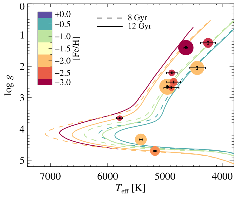
Figure 1: Stellar parameters of our ten metal-poor stars, colour-coded by metallicity, compared to theoretical Dartmouth isochrones of different ages (linestyles) and metallicities (colours). Formal $1\sigma$ uncertainties are shown by the error bars. The symbol size is proportional to the angular diameter of the star.

2 Observations

2.1 Science targets

The ten metal-poor stars considered in this work have metallicities between $[\mathrm{Fe/H}]$ = $-$0.7 and $-$2.6. The stars are HD 2665, HD 6755, HD 6833, HD 103095, HD 122563, HD 127243, HD 140283, HD 175305, HD 221170 and HD 224930. These stars are candidates for benchmarks used for validating large stellar surveys. The sample spans the entire evolutionary range of solar mass metal poor stars as seen in Fig. 1, and we list their astrometric parameters in Table 1.

We selected the ten stars in consultation with the Gaia-ESO spectroscopic team. The stars have sizes and brightness such that their angular diameters can be measured reliably using the chosen interferometric instrument, and thus the $T_{\mathrm{eff}}$ can be inferred reliably.

Three of the stars, HD 103095, HD122563, and HD 140283, are currently used as Gaia FGK benchmark stars (Heiter et al., 2015). In the previous paper (Karovicova et al., 2018) the reliability of the approach was demonstrated on these three stars. They are again included here because the data reduction have been updated, and in order to present a homogeneous set of stellar parameters for all ten stars.

The other seven stars have not previously been used as benchmark stars. HD 175303 was discussed in an update to the Gaia FGK benchmarks (Hawkins et al., 2016). Four stars (HD 2665, HD 6755, HD 6833, HD 221170) were suggested in the conclusion of Heiter et al. (2015), on the basis of their inclusion in the catalogue of hydrogen line profiles from Huang et al. (2012). We moreover added two targets (HD 127243 and HD 224930) with slightly higher metallicities (-0.7 dex), which according to the PASTEL catalogue (Soubiran et al., 2010a), are thought to be typical stars and serve to complete the sample.

Table 1: Astrometric parameters

Star	Right ascension	Declination	mV	mR	$E(B-V)$	$\pi$ a
			(mag)	(mag)		(mas)
HD 2665	00 30 45.447	$+$57 03 53.627	7.72	7.74	0.049 $\pm$ 0.02	3.714 $\pm$ 0.036
HD 6755	01 09 43.060	$+$61 32 50.293	7.68	7.30	0.010 $\pm$ 0.01	5.969 $\pm$ 0.049
HD 6833	01 09 52.265	$+$54 44 20.273	6.74	6.77	0.047 $\pm$ 0.02	4.711 $\pm$ 0.048
HD 103095	11 52 58.768	$+$37 43 07.240	6.45	5.80	0 $\pm$ 0	108.955 $\pm$ 0.049
HD 122563	14 02 31.846	$+$09 41 09.943	6.19	5.37	0.003 $\pm$ 0.01	3.440 $\pm$ 0.063
HD 127243	14 28 37.813	$+$49 50 41.461	5.59	5.10	0 $\pm$ 0	10.390 $\pm$ 0.069
HD 140283	15 43 03.097	$-$10 56 00.596	7.12	6.63	0 $\pm$ 0	16.144 $\pm$ 0.072
HD 175305	18 47 06.442	$+$74 43 31.448	7.18	6.52	0.010 $\pm$ 0.01	6.349 $\pm$ 0.025
HD 221170	23 29 28.809	$+$30 25 57.847	7.66	7.69	0.061 $\pm$ 0.02	1.837 $\pm$ 0.059
HD 224930	00 02 10.341	$+$27 04 54.477	5.75	5.16	0 $\pm$ 0	79.070 $\pm$ 0.560

Table 2: Interferometric observations - metal-poor stars

Science target	UT date	Telescope	B (m) )	# of obs.	Calibrator stars
HD 2665	2016 Aug 11	E1W1	313.57	3	HD 584, HD 3519
	2016 Aug 13	E1W2	221.85	2	HD 584, HD 3519
	2016 Aug 17	E2W1	251.34	1	HD 584, HD 3519
	2016 Oct 7	E2W1	251.34	5	HD 584, HD 3519
HD 6755	2016 Aug 11	E1W1	313.57	2	HD 3519, HD 9878
	2016 Aug 17	E2W1	251.34	3	HD 3519, HD 9878
	2016 Oct 7	E2W1	251.34	6	HD 3519, HD 9878
HD 6833	2009 Jul 17	W1W2	107.93	2	HD 6028
	2009 Jul 21	S2W2	177.45	2	HD 6676
	2015 Sep 25	E2W2	156.26	3	HD 3519, HD 3802, HD 7804
HD 103095a	2015 May 2	E2W2	156.26	3	HD 99002, HD 103288
	2017 Mar 3	E2W2	156.26	3	HD 99002, HD 107053
		E2W1	251.34	2	HD 99002, HD 107053
	2017 Mar 4	E1W2	221.85	3	HD 99002, HD 103288, HD 107053
HD 122563a	2017 Mar 3	E2W2	156.26	3	HD 120448, HD 122365, HD 128481
	2017 June 9	E2W2	156.26	2	HD 121996, HD 128481
	2017 June 10	E2W2	156.26	2	HD 120934
HD 127243	2015 Apr 5	W1W2	107.93	3	HD 122866, HD 125349, HD 128184
	2015 Jul 27	E2W2	156.26	2	HD 10 128998, HD 133962, HD 140728
HD 140283a	2014 Apr 8	E1W1	313.57	4	HD 139909, HD 143259, HD 146214
	2015 Apr 4	S1W1	278.50	2	HD 139909, HD 143259
	2017 June 16	E1W1	313.57	4	HD 128481, HD 143259
HD 175305	2015 Jul 28	E2W2	156.26	3	HD 157774, HD 169027
	2015 Sep 21	E1W2	221.85	4	HD 146929, HD 157774, HD 169027
	2015 Sep 23	E1W2	221.85	2	HD 146929, HD 169027
	2015 Sep 24	E2W2	156.26	4	HD 169027, HD 178738, HD 197637
HD 221170	2009 Jul 20	S2W2	177.45	3	HD 221491
	2015 Sep 8	E1W2	221.85	1	HD 220599
	2016 Aug 10	E2W2	156.26	3	HD 220599, HD 221491
	2016 Aug 13	E1W2	221.85	3	HD 220599, HD 221491
	2016 Oct 7	E2W1	251.34	2	HD 220599, HD 221491
HD 224930	2015 Aug 6	S2W2	177.45	3	HD 1439
	2015 Aug 7	E2W2	156.26	3	HD 1439, HD 1606

2.2 Interferometric observations and data reduction

We observed the stars using the interferometric instrument PAVO (Ireland et al., 2008). The instrument is located at the CHARA array at Mt. Wilson Observatory, California (ten Brummelaar et al., 2005). The PAVO instrument is operating in optical wavelengths between $\sim$ 600–900 nm and it is a pupil-plane beam combiner. The PAVO instrument is limited to observations of targets with magnitudes of m_R $\sim$ 7.5. In the case of ideal weather conditions, it is possible to observe targets down to m_R=8, with recent improvements due to adaptive optics (Che et al., 2014). The CHARA array offers the longest available baselines in the optical wavelengths worldwide. The stars were observed using baselines between 107.9 m and 313.6 m. We collected the observations between 2009 Jul 17 and 2016 Oct 7. Table 2 summarizes our dates of observations, telescope configuration and the projected baselines B.

The data were reduced with the PAVO reduction software. The PAVO data reduction software has been well-tested and used in multiple studies (Bazot et al., 2011; Derekas et al., 2011; Huber et al., 2012; Maestro et al., 2013). In order to monitor the interferometric transfer function, a set of calibrating stars were observed. These calibrating stars were selected from a catalogue of CHARA calibrators and from the Hipparcos catalogue (ESA, 1997). According to the location and sizes of an observed target we selected unresolved or closely unresolved sources, located close on the sky to the science target. The calibrating stars were observed immediately before as well as after the science target. We determined the angular diameters of the calibrators using the $V-K$ relation of Boyajian et al. (2014) and corrected for limb-darkening to determine the uniform disc diameter in $R$ band. The $V$-band magnitudes were selected from the Tycho-2 catalogue (Høg et al., 2000) and converted into the Johnson system using the calibration by Bessell (2000). The $K$-band magnitudes were selected from the Two Micron All Sky Survey (2MASS; Skrutskie et al., 2006). The reddening was estimated from the dust map of Green et al. (2015) and the reddening law of O’Donnell (1994) was applied. We set the relative uncertainty on calibrator diameters to 5% (Boyajian et al., 2014). The uncertainty is set in a way that it covers the uncertainty on the calibrator diameters as well as the uncertainty on the reddening. We also set the absolute uncertainty on the wavelength scale to 5 nm. We checked the literature for each calibrator to ensure they were not known binaries. According to Gaia DR2, both the proper motion anomaly (Kervella et al., 2019) and the $\rm{\tt phot\_bp\_rp\_excess\_factor}$ (Evans et al., 2018) suggest that none of our calibrators has a companion that is large enough to affect our interferometric measurements or estimated calibrator sizes. We note that for the smallest science targets, such as HD 2665 and HD 6755, we have endeavored to choose the smallest calibrators that were practical, which in these cases were $<$ 0.15 mas. For all the calibrating stars, their spectral type, magnitude in the $V$ and $R$ band, their expected angular diameter and the corresponding science targets are summarized in Table 3.

Table 3: Calibrator stars used for interferometric observations - metal-poor stars

Calibrator	Spectral	mV	mK	$E(B-V)$	UD
	type			(mag)	(mas)
HD 584	B8III	6.72	6.97	0.113	0.126
HD 1439	A0IV	5.88	5.86	0.042	0.221
HD 1606	B7V	5.87	6.23	0.050	0.177
HD 3519	A0	6.72	6.74	0.093	0.145
HD 3802	A0	6.73	6.57	0.008	0.164
HD 6028	A3V	6.47	6.01	0.023	0.221
HD 6676	B8V	5.77	5.75	0.049	0.233
HD 7804	A1V	5.14	4.92	0.008	0.353
HD 9878	B7V	6.71	6.70	0.185	0.145
HD 99002	F0	6.93	6.28	0.008	0.201
HD 103288	F0	7.00	6.22	0.006	0.211
HD 103928	A9V	6.42	5.60	0.002	0.282
HD 107053	A5V	6.68	6.02	0.004	0.226
HD 120448	A0	6.78	6.52	0.017	0.169
HD 120934	A1V	6.10	5.96	0.007	0.216
HD 121996	A0Vs	5.76	5.70	0.029	0.238
HD 122365	A2V	5.98	5.70	0.007	0.248
HD 122866	A2V	6.15	6.11	0.005	0.199
HD 125349	A2IV	6.20	5.98	0.002	0.217
HD 128184	A0	6.51	6.29	0.009	0.188
HD 128481	A0	6.98	6.79	0.007	0.149
HD 128998	A1V	5.82	5.76	0.009	0.235
HD 133962	A0V	5.58	5.61	0.003	0.249
HD 139909	B9.5V	6.86	6.54	0.110	0.165
HD 140728	A0V	5.48	5.56	0.008	0.253
HD 143259	B9V	6.64	6.28	0.107	0.187
HD 146214	A1V	7.49	7.10	0.012	0.132
HD 146926	B8V	5.48	5.70	0.014	0.233
HD 157774	A0	7.13	7.01	0.011	0.133
HD 169027	A0	6.79	6.95	0.011	0.132
HD 178738	A0	6.89	6.85	0.036	0.141
HD 197637	B3	6.94	7.35	0.107	0.104
HD 220599	B9III	5.55	5.72	0.010	0.232
HD 221491	B8V	6.64	6.75	0.034	0.145

Table 4: Angular diameters and linear limb-darkening coefficients.

Star	$\theta_{\mathrm{UD}}$ (mas)	Linear limb darkeninga
		$u$	$\theta_{\mathrm{LD}}$ (mas)
HD 2665	0.377 $\pm$ 0.004	0.561 $\pm$ 0.009	0.397 $\pm$ 0.003
HD 6755	0.354 $\pm$ 0.004	0.575 $\pm$ 0.014	0.375 $\pm$ 0.004
HD 6833	0.804 $\pm$ 0.009	0.674 $\pm$ 0.011	0.862 $\pm$ 0.009
HD 103095	0.565 $\pm$ 0.004	0.565 $\pm$ 0.016	0.597 $\pm$ 0.005
HD 122563	0.861 $\pm$ 0.010	0.568 $\pm$ 0.009	0.907 $\pm$ 0.011
HD 127243	0.922 $\pm$ 0.006	0.621 $\pm$ 0.013	0.983 $\pm$ 0.008
HD 140283	0.311 $\pm$ 0.005	0.510 $\pm$ 0.003	0.326 $\pm$ 0.006
HD 175305	0.461 $\pm$ 0.006	0.590 $\pm$ 0.014	0.487 $\pm$ 0.006
HD 221170	0.563 $\pm$ 0.005	0.632 $\pm$ 0.014	0.599 $\pm$ 0.006
HD 224930	0.680 $\pm$ 0.007	0.566 $\pm$ 0.014	0.720 $\pm$ 0.007

Table 5: Observed ($\varTheta_{LD}$) and derived ($F_{\mathrm{bol}}$, $M$, $L$, $R$) stellar parameters

Star	$F_{\mathrm{bol}}$	$\varTheta_{LD}$	Mass (M⊙)	$L$ (L⊙)	$R$ (R⊙)
	(erg s-1cm-210-8)	(mas)
HD 2665	2.95 $\pm$ 0.22	0.395 $\pm$ 0.004	0.77 $\pm$ 0.05	66.4 $\pm$ 5.2	11.43 $\pm$ 0.16
HD 6755	2.59 $\pm$ 0.27	0.369 $\pm$ 0.004	0.78 $\pm$ 0.05	22.7 $\pm$ 2.4	6.648 $\pm$ 0.090
HD 6833	9.4 $\pm$ 1.2	0.852 $\pm$ 0.008	1.00 $\pm$ 0.15	152.6 $\pm$ 5.8	19.45 $\pm$ 0.27
HD 103095	8.41 $\pm$ 0.18	0.593 $\pm$ 0.004	0.63 $\pm$ 0.02	0.221 $\pm$ 0.005	0.586 $\pm$ 0.004
HD 122563	13.14 $\pm$ 0.22	0.925 $\pm$ 0.011	0.77 $\pm$ 0.05	339 $\pm$ 13	28.86 $\pm$ 0.63
HD 127243	18.99 $\pm$ 0.18	0.971 $\pm$ 0.007	1.46 $\pm$ 0.15	54.97 $\pm$ 0.90	10.045 $\pm$ 0.098
HD 140283	3.955 $\pm$ 0.029	0.325 $\pm$ 0.006	0.77 $\pm$ 0.03	4.766 $\pm$ 0.055	2.167 $\pm$ 0.041
HD 175305	4.33 $\pm$ 0.41	0.484 $\pm$ 0.006	0.78 $\pm$ 0.05	33.5 $\pm$ 3.2	8.20 $\pm$ 0.11
HD 221170	3.85 $\pm$ 0.46	0.596 $\pm$ 0.005	0.79 $\pm$ 0.05	3567 $\pm$ 48	34.86 $\pm$ 1.16
HD 224930	14.76 $\pm$ 0.10	0.716 $\pm$ 0.007	0.75 $\pm$ 0.01	0.741 $\pm$ 0.012	0.973 $\pm$ 0.012

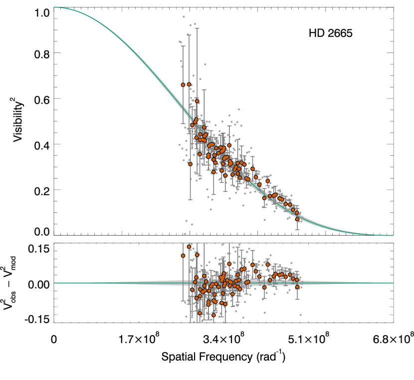
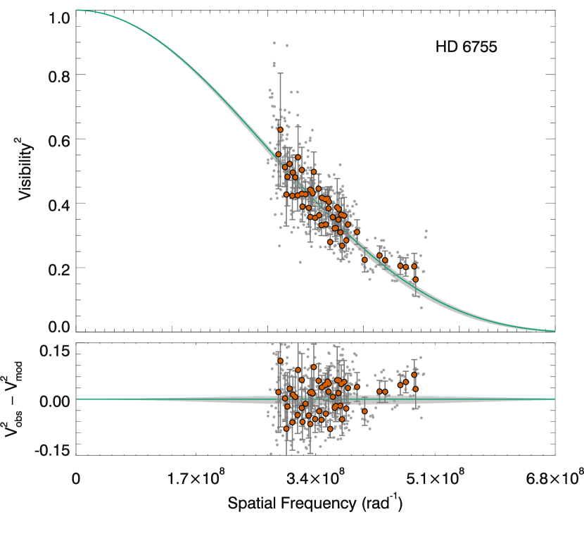
Figure 2: Squared visibility versus spatial frequency for HD 2665 and HD 6755. The HD number is noted in the right upper corner in the each plot. The error bars have been scaled to the reduced $\chi^{2}$. For HD 2665 the reduced $\chi^{2}$ = 1.6 and for HD 6755 $\chi^{2}$ = 1.7. The grey dots are the individual PAVO measurements in each wavelength channel. For clarity, we show weighted averages of the PAVO measurements as red circles. The green line shows the fitted limb-darkened model to the PAVO data, with the light grey-shaded region indicating the 1-$\sigma$ uncertainties. The lower panel shows the residuals from the fit.

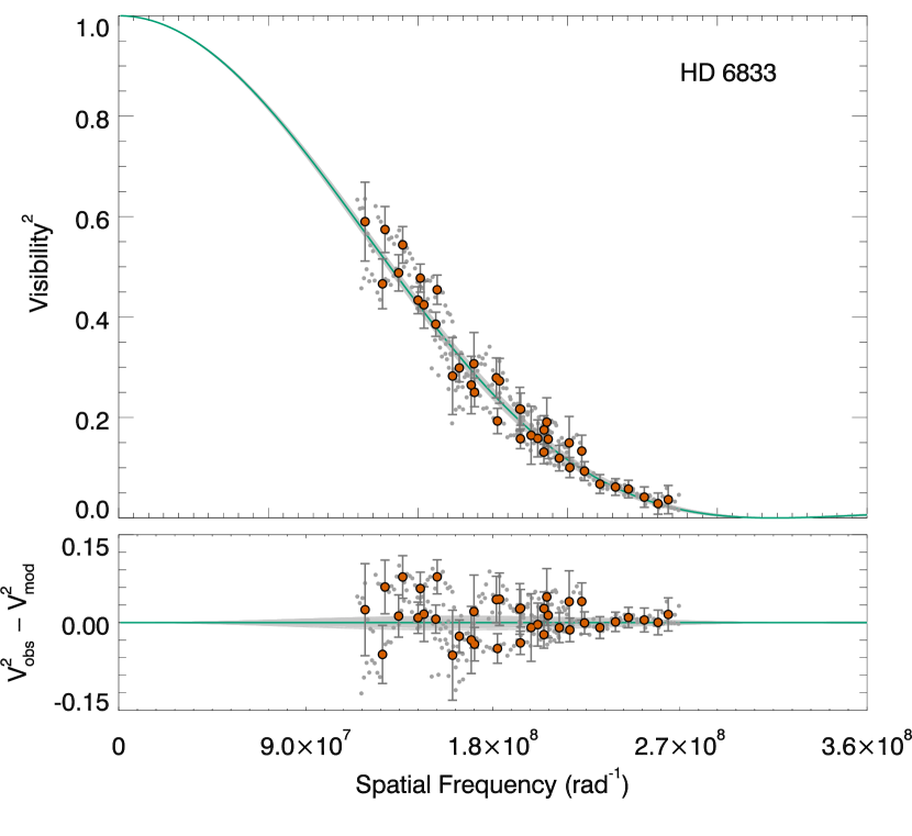
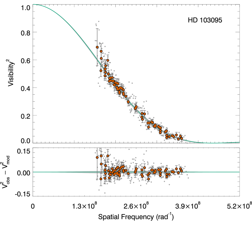
Figure 3: Squared visibility versus spatial frequency for HD 6833 and HD 103095. The lower panel shows the residuals from the fit. The error bars have been scaled to the reduced $\chi^{2}$. For HD 6833 the reduced $\chi^{2}$ = 7.0 and for HD 103095 $\chi^{2}$ = 1.1. All lines and symbols are the same as for Fig.2.

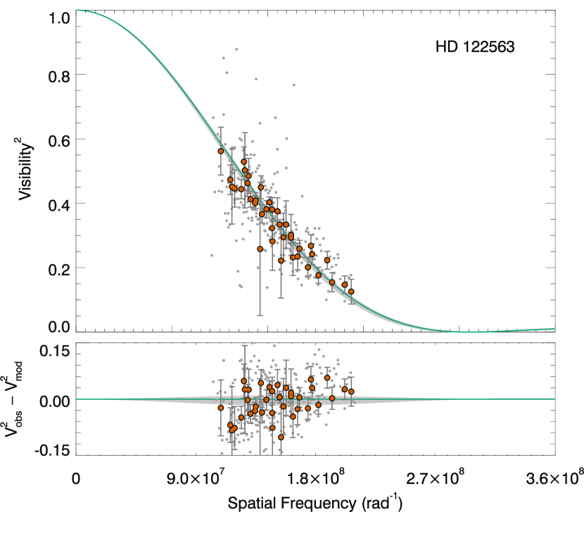
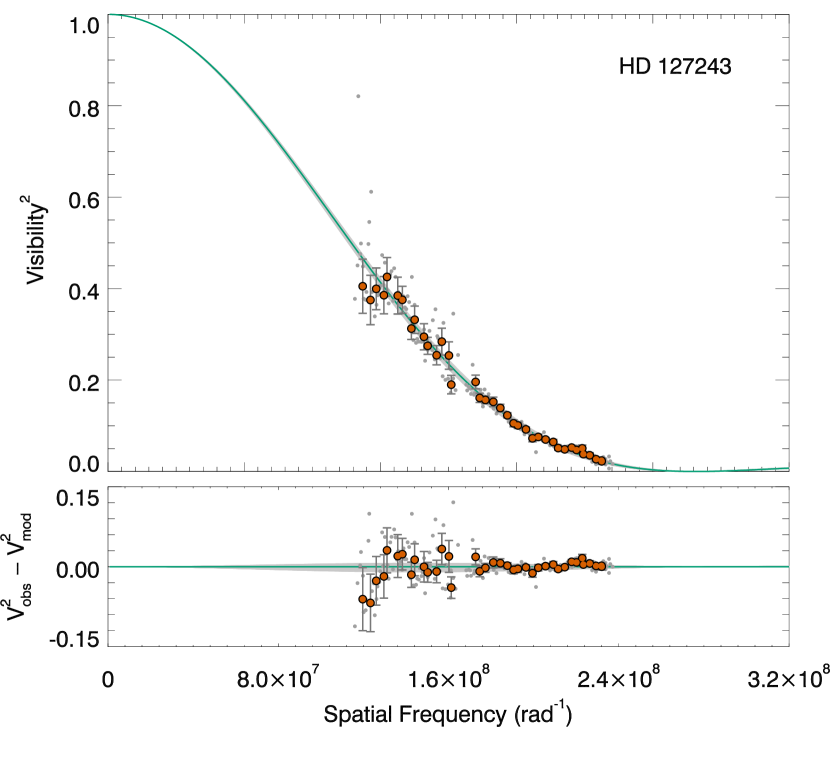
Figure 4: Squared visibility versus spatial frequency for HD 122563 and HD 127243. The lower panel shows the residuals from the fit. The error bars have been scaled to the reduced $\chi^{2}$. For HD 122563 the reduced $\chi^{2}$ = 3.0 and for HD 127243 $\chi^{2}$ = 1.6. All lines and symbols are the same as for Fig.2.

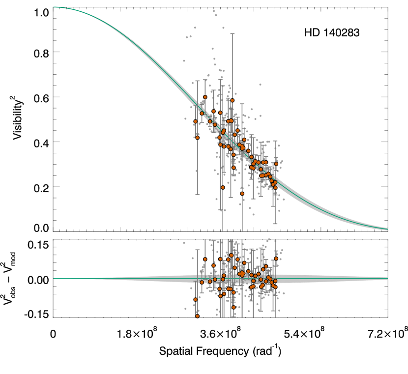
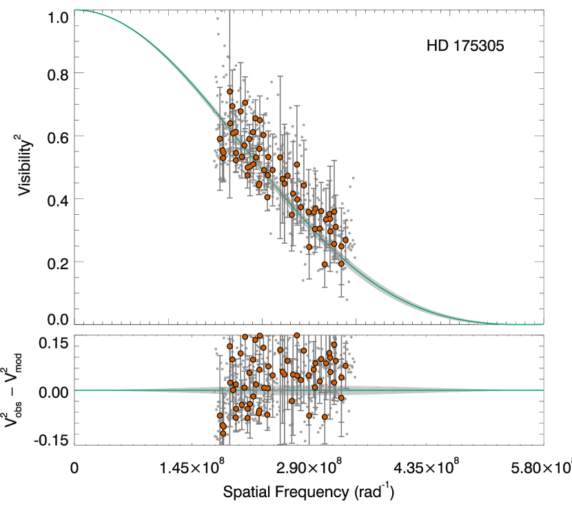
Figure 5: Squared visibility versus spatial frequency for HD 140283 and HD 175305. The lower panel shows the residuals from the fit. The error bars have been scaled to the reduced $\chi^{2}$. For HD 140283 the reduced $\chi^{2}$ = 1.4 and for HD 175305 $\chi^{2}$ = 3.7. All lines and symbols are the same as for Fig.2.

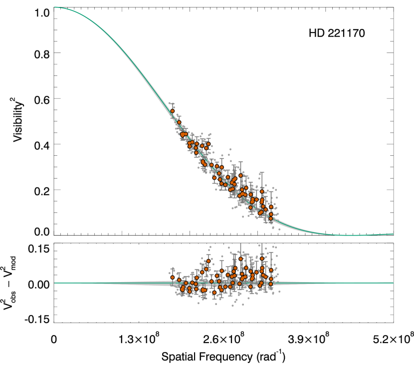
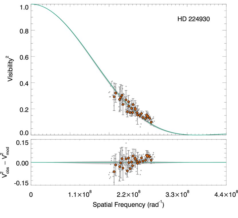
Figure 6: Squared visibility versus spatial frequency for HD 221170 and HD 224930. The lower panel shows the residuals from the fit. The error bars have been scaled to the reduced $\chi^{2}$. For HD 221170 the reduced $\chi^{2}$ = 2.1 and for HD 224930 $\chi^{2}$ = 8.4. All lines and symbols are the same as for Fig.2.

3 Methods and analysis

In the following section we describe the method delivering the stellar parameters, showing the connection between the interferometric, photometric and spectroscopic analysis. To obtain the angular diameter (see below), and hence the $T_{\mathrm{eff}}$, from the interferometric data requires a limb-darkening parameter. This depends on $T_{\mathrm{eff}}$, $\log(g)$ and $[\mathrm{Fe/H}]$. The process of estimating the $T_{\mathrm{eff}}$ is thus initiated by entering a first guess for the stellar parameters (from the literature), and linearly interpolating the limb-darkening coefficients from the STAGGER-grid (Magic et al., 2015).

The first limb-darkened angular diameter together with the bolometric flux allows to directly compute the $T_{\mathrm{eff}}$ (equation 1). The $\log(g)$ and $[\mathrm{Fe/H}]$ were then refined by isochrone fitting and spectroscopic analysis: $\log(g)$ is sensitive to $T_{\mathrm{eff}}$ and metallicity, and $[\mathrm{Fe/H}]$ is sensitive to $T_{\mathrm{eff}}$ and log(g), therefore, these values are slightly refined with each iteration. The final values of fundamental stellar parameters of the benchmark stars were iterated between interferometric, photometric, and spectroscopic modelling, until convergence was reached.

We did not encounter any major convergence problems. Changing the initial guess parameters by 500 K in $T_{\mathrm{eff}}$, 0.2 dex in log(g), or 0.2 dex in [Fe/H] did not change the final converged angular diameter result (to within the $1\sigma$ errors).

3.1 Modelling of limb-darkened angular diameters

The determination of accurate angular diameters requires an estimate of an appropriate amount of limb-darkening derived from stellar model atmospheres. As a first step, we fitted to the visibility curves an undarkened uniform disc. For all our fits, both with and without limb-darkening, we used a least-squares fitting routine in IDL (MPFIT, Markwardt, 2009), with uncertainties being determined by Monte Carlo simulations that took into account the uncertainty in the visibility measurements, as well as the wavelength calibration (5 nm), calibrator sizes (5%) and, for the limb-darkened fits, the limb-darkening coefficients.

Our fitted uniform disk diameters are listed in Table 3. We also fitted the commonly used linear limb-darkening law from Claret & Bloemen (2011); these are grids of coefficients calculated for various model atmospheres and different photometric filters. For reference, we also present the resulting limb-darkened angular diameters in Table 3. However, we stress that our final $T_{\mathrm{eff}}$ estimates are based on high-order limb-darkening coefficients from the STAGGER-grid. The 3D hydrodynamical models have been shown to better reproduce the solar limb darkening than both theoretical and semi-empirical 1D hydrostatic models (Pereira et al., 2013). For this reason, they are expected to give better overall results and are adopted in the present analysis. The final results based on the STAGGER-grid are presented in Table 5, and discussed below.

For robust estimates and accurate angular diameter we employed higher-order limb-darkening laws. The method used in this study generally follows the same procedure described in Section 2.2 in the previous study of the same topic in Karovicova et al. (2018). In short, we employed the four-parameter limb-darkening coefficients of Magic et al. (2015), that were calculated from 3D synthetic spectra from Chiavassa et al. (2018) for the STAGGER-grid of ab initio 3D hydrodynamic stellar atmosphere simulations (Magic et al., 2013). These coefficients are tabulated as functions of $T_{\mathrm{eff}}$, $\log(g)$ and $[\mathrm{Fe/H}]$; we interpolated them based on our initial guesses, and refined them using our measurements of $T_{\mathrm{eff}}$ based on the bolometric flux (Section 3.2), $\log(g)$ based on stellar evolution models (Section 3.3), and $[\mathrm{Fe/H}]$ based on spectroscopy (Section 3.4). We note that for one of our stars, HD 221170, its $\log(g)$ value places it outside the STAGGER-grid. For this star we therefore linearly extrapolated its coefficients from the STAGGER-grid, and confirmed that these provided reasonable values by comparing them with coefficients from the tables of Claret & Bloemen (2011). Using 3D models instead of 1D models generally has a very small effect on the determined limb darkened angular diameters, compared to the error bars, indicating that the measurements are usually only mildly dependent on the model assumptions. However, in the worst case (HD 122563) the differences are 2%, that translates into 1% in $T_{\mathrm{eff}}$ which is the targeted precision. We present the limb darkening coefficients from the STAGGER-grid (in all 38 channels) in Tables 9-18 available at the CDS.

3.2 Bolometric flux

Many of the stars in the sample have saturated or unreliable 2MASS photometry, which prevents us from using the InfraRed Flux Method to derive bolometric fluxes (Casagrande et al., 2010). Hence, for all targets we use bolometric corrections from Casagrande & VandenBerg (2014); Casagrande & VandenBerg (2018b). We use Hipparcos $H_{p}$ and Tycho2 $B_{T}V_{T}$ magnitudes for all stars, and 2MASS $JHK_{S}$ only if with quality flag ‘A’. We assumed no reddening for all stars closer than 100 pc; for stars further away we estimated $E(B-V)$ using interstellar Na I D lines when possible, or the Green et al. (2015) map otherwise.

Tables of bolometric corrections were interpolated at the adopted reddening, and spectroscopic $[\mathrm{Fe/H}]$ and $\log(g)$. Spectroscopic $T_{\mathrm{eff}}$ were used only as a starting point to interpolate bolometric corrections. The adopted bolometric corrections are listed in Table 5. An iterative procedure was adopted, where the bolometric corrections were used together with the angular diameter to derive an updated $T_{\mathrm{eff}}$ until convergence was reached to within a few K.

The bolometric flux was obtained using a weighted average of the bolometric flux from the bolometric correction in each band. Weights were given by the inverse of the estimated variance of the bolometric flux derived from each band. These were obtained for each photometric band by computing the mean square deviation using a Monte Carlo integration over four independent parameters ($T_{\mathrm{eff}}$, $\log(g)$, $[\mathrm{Fe/H}]$ and $E(B-V)$) and the photometric magnitude for that band. All five input parameters errors were modelled as independent normally distributed random variables. The uncertainties quoted for the bolometric flux are the square root of the weighted sample variance, plus a 0.3% systematic to account for the uncertainty in the adopted reference solar luminosity. The systematic uncertainties and inaccuracies stemming from the use of model fluxes are harder to quantify, but extensive comparison with absolute spectrophotometry in Casagrande & VandenBerg (2018a) indicates that bolometric fluxes are typically recovered at the percent level for FG stars. Our sample comprises cooler stars, for which the performances of our bolometric corrections are much less tested. Reassuringly, the comparison of our bolometric corrections with absolute spectrophotometry from White et al. (2018) also indicates good agreement for stars in the $T_{\mathrm{eff}}$ range covered by the present work.

Table 6: Bolometric corrections

Star	BC${}_{H_{p}}$	BC${}_{B_{T}}$	BC${}_{V_{T}}$	BCJ	BCH	BCK	$B_{T}$	e$B_{T}$	$V_{T}$	e$V_{T}$	$H_{p}$	e$H_{p}$	$J$	e$J$	$H$	e$H$	$K$	e$K$
HD 2665	-0.622	-1.494	-0.592	1.306	1.827	1.949	8.649	0.016	7.813	0.010	7.8637	0.0009	6.026	0.024	5.603	0.033	5.474	0.016
HD 6755	-0.489	-1.324	-0.453	1.334	1.842	1.955	8.586	0.016	7.808	0.010	7.8620	0.0015	6.197	0.024	5.759	0.020	5.662	0.017
HD 6833	-0.828	-2.135	-0.814	1.455	2.107	2.256	8.245	0.015	6.892	0.009	6.9110	0.0007	-	-	-	-	-	-
HD 103095	-0.357	-1.105	-0.318	1.258	1.682	1.786	7.353	0.015	6.509	0.010	6.5641	0.0009	-	-	-	-	4.373	0.027
HD 122563	-0.603	-1.597	-0.578	1.438	2.008	2.116	7.275	0.015	6.304	0.009	6.3275	0.0007	-	-	-	-	-	-
HD 127243	-0.415	-1.314	-0.369	1.345	1.824	1.931	6.655	0.014	5.681	0.009	5.7362	0.0005	-	-	-	-	-	-
HD 140283	-0.278	-0.739	-0.244	1.017	1.345	1.421	7.771	0.016	7.269	0.011	7.3000	0.0013	6.014	0.019	5.696	0.036	5.588	0.017
HD 175305	-0.501	-1.372	-0.465	1.350	1.871	1.983	8.109	0.015	7.275	0.010	7.3211	0.0006	5.613	0.023	5.167	0.024	5.057	0.020
HD 221170	-1.050	-2.501	-1.062	1.495	2.204	2.368	8.990	0.018	7.797	0.011	7.8373	0.0009	5.532	0.018	4.987	0.044	4.836	0.016
HD 224930	-0.281	-0.967	-0.234	1.186	1.560	1.648	6.555	0.014	5.834	0.009	5.8735	0.0009	-	-	-	-	-	-

3.3 Stellar evolution models

We used the ELLI package (Lin et al., 2018) to estimate stellar masses based on comparisons to Dartmouth stellar evolution tracks (Dotter et al., 2008), computed with alpha enhancement. The comparison uses a Bayesian framework to estimate the stellar mass and age from $T_{\mathrm{eff}}$, $\log L/L_{\odot}$ and $[{\rm Fe}/{\rm H}]$, taking into account their related (assumed independent) errors. An initial guess is produced from a maximum likelihood estimate at our estimated metallicity, between the fundamental stellar parameters and those estimated on the isochrone. A Markov chain Monte Carlo (MCMC) method is then used to sample the posterior distribution, and we take the mean and dispersion on this distribution as our estimate for the mass and its uncertainty. Finally, we compute the surface gravity from its fundamental relation, rewritten to a form that directly utilises the measurements,

$$\log g=\log\frac{GM}{R^{2}}=\log\frac{4GM\varpi^{2}}{\theta^{2}},$$ (2)

where $G$ is the gravitational constant and $\varpi$ the parallax.

As shown in Fig 1, there are systematic offsets between the theoretical stellar isochrones and the parameters of metal-poor stars on the red giant branch. Our Bayesian sampling approach therefore does a poor job of predicting the properties of these stars. Instead, we adopted the turnoff-mass at the relevant metallicity and assuming an age $>10$ Gyr. Since we did not use the Bayesian approach for these stars, we use instead a conservative uncertainty estimate on the stellar mass of 0.05 $M_{\odot}$.

3.4 Spectroscopic analysis

High-resolution spectra for the stars were extracted from the ELODIE ($R\approx 42\,000$, Moultaka et al., 2004) and FIES ($R\approx 65\,000$, Telting et al., 2014) archives. We determined the stellar iron abundances using a custom pipeline based on the spectrum synthesis code SME (Piskunov & Valenti, 2017) using MARCS model atmospheres (Gustafsson et al., 2008) and pre-computed non-LTE departure coefficients for Fe (Amarsi et al., 2016).

We selected unblended lines of Fe i and Fe ii between 4400 and 6800 Å with accurately known oscillator strengths from laboratory measurements. For saturated lines, we ensured that collisional broadening parameters were available from ABO theory (Barklem et al., 2000; Barklem & Aspelund-Johansson, 2005). To obtain a differential $[\mathrm{Fe/H}]$, solar abundances were also measured from solar spectra recorded with the same spectrographs as our target stars, based on observations of light reflected off the Moon (ELODIE) and Vesta (FIES). We thereby produce solar-differential abundances, which mostly cancels uncertainties in oscillator strengths as well as potential systematic differences between the spectrographs. We estimated the iron abundance of each star from the outlier-resistant mean of the entire set of Fe I and Fe II lines, with $3\sigma$ clipping. We also computed the difference in abundance between lines of Fe i and Fe ii, as an estimate of how closely our fundamental stellar parameters fulfill the ionization equilibrium. Finally, we compute a systematic uncertainty on the metallicity, that we derive by perturbing the input parameters one at a time according to their formal errors, and add these differences in quadrature.

Table 7: Derived stellar parameters ($T_{\mathrm{eff}}$ , $[\mathrm{Fe/H}]$, $\log(g)$)

Star	$T_{\mathrm{eff}}$	$\log(g)$	$[\mathrm{Fe/H}]$
	(K)	(dex)	(dex)
HD 2665	4883 $\pm$ 95	2.209 $\pm$ 0.032	$-$2.10 $\pm$ 0.09 $\pm$ 0.10
HD 6755	4888 $\pm$ 131	2.685 $\pm$ 0.031	$-$1.71 $\pm$ 0.10 $\pm$ 0.14
HD 6833	4438 $\pm$ 141	1.860 $\pm$ 0.072	$-$0.80 $\pm$ 0.07 $\pm$ 0.04
HD 103095	5174 $\pm$ 32	4.702 $\pm$ 0.015	$-$1.26 $\pm$ 0.07 $\pm$ 0.02
HD 122563	4635 $\pm$ 34	1.404 $\pm$ 0.035	$-$2.75 $\pm$ 0.12 $\pm$ 0.04
HD 127243	4959 $\pm$ 21	2.599 $\pm$ 0.047	$-$0.71 $\pm$ 0.06 $\pm$ 0.02
HD 140283	5792 $\pm$ 55	3.653 $\pm$ 0.024	$-$2.29 $\pm$ 0.10 $\pm$ 0.04
HD 175305	4850 $\pm$ 118	2.502 $\pm$ 0.031	$-$1.52 $\pm$ 0.08 $\pm$ 0.12
HD 221170	4248 $\pm$ 128	1.251 $\pm$ 0.042	$-$2.40 $\pm$ 0.13 $\pm$ 0.17
HD 224930	5422 $\pm$ 28	4.337 $\pm$ 0.012	$-$0.81 $\pm$ 0.05 $\pm$ 0.02

Table 8: Uncertainties in $T_{\mathrm{eff}}$ and how they propagate from the underlying measurements

Star	$T_{\mathrm{eff}}$	e$T_{\mathrm{eff}}$	e$F_{\mathrm{bol}}$ a	e$\varTheta_{LD}$ b
	(K)	(K)	(K)	(K)
HD 2665	4883	95	92	25
HD 6755	4888	131	128	26
HD 6833	4438	141	139	21
HD 103095	5174	32	27	17
HD 122563	4635	34	19	28
HD 127243	4959	21	12	18
HD 140283	5792	55	11	54
HD 175305	4850	118	114	30
HD 221170	4248	128	126	18
HD 224930	5422	28	9	27

4 Results and discussion

4.1 Recommended stellar parameters

We presented fundamental stellar parameters and angular diameters for a set of benchmark stars. Four of the ten stars are Gaia FGK benchmark stars (HD 12256, HD 103095, HD 140283, HD 175305). Six of the stars (HD 2665, HD 6755, HD 6833, HD 221170, HD 127243, HD 224930) were added and suggested as new benchmark stars. For all stars we estimated $T_{\mathrm{eff}}$, log$g$, $[\mathrm{Fe/H}]$ and $\theta$_LD. All the values along with mass, luminosity and radii are summarized in Table 5.

4.2 Uncertainties

The final $T_{\mathrm{eff}}$ uncertainties consist of uncertainties in the bolometric flux and the uncertainties in the angular diameter. Table 8 shows the contribution of each part. The third column shows the final $T_{\mathrm{eff}}$ uncertainties, the fourth column the uncertainties raising from the bolometric flux if the $\varTheta_{LD}$ uncertainties are set to 0. The fifth column shows the $F_{\mathrm{bol}}$ uncertainties set to 0, with the uncertainties raising entirely from the angular diameter.

The statistical measurement uncertainties in $\log(g)$ and $\mathrm{[Fe/H]}$ from the isochrone fitting and spectroscopic analysis were folded into the uncertainties of the angular diameters and thus are included in the final $T_{\mathrm{eff}}$ error estimates. The median uncertainties in $\log(g)$ and $\mathrm{[Fe/H]}$ across our sample of stars are 0.03 dex and 0.09 dex, respectively (Table 7).

For five of the stars, the final $T_{\mathrm{eff}}$ uncertainties are less than around 50 K, or 1%. For these stars, the errors coming from the bolometric flux are less than or similar to those coming from the limb-darkened angular diameter. The final $T_{\mathrm{eff}}$ uncertainties for the other five stars are somewhat larger: 100–150 K. This is driven by larger errors in the bolometric flux, rather than in the angular diameter. As mentioned above, the precision that is desired by the spectroscopic teams of surveys like Gaia-ESO or GALAH is around 1% (or around 40-60 K); we achieve this for half of our sample, and could achieve it for the full sample if more precise bolometric fluxes are available.

4.3 Comparison with literature values

Three of our ten targets (HD 103095, HD 122563 and HD 140283) were previously interferometrically studied by Creevey et al. (2012, 2015) and they are also a part of the previous interferometric study (Karovicova et al., 2018). These stars were used as Gaia FGK benchmark stars in the Gaia-ESO spectroscopic survey. However, the stars HD 103095, and HD 140283 had to be reconsidered as their $T_{\mathrm{eff}}$ did not reconcile with spectroscopic studies. Therefore, the stars were not recommended as temperature standards until discrepancies are resolved (see Heiter et al., 2015). The issues were resolved in Karovicova et al. (2018) and the stars can be now again used as benchmarks.

HD 103095 This star was interferometrically observed by Creevey et al. (2012), who reported $T_{\mathrm{eff}}$=4818$\pm$54 K. This value is lower than a value estimated in the previous study (Karovicova et al., 2018) where $T_{\mathrm{eff}}$=5140$\pm$49 K was determined. Here with our improved reduction method we obtain $T_{\mathrm{eff}}$=5174$\pm$32, log$g$=4.702$\pm$0.015 dex and $[\mathrm{Fe/H}]$=$-$1.26$\pm$0.07 dex; note all the differences with the previous study are within the stipulated uncertainties.

HD 122563 This metal-poor star is well studied spectroscopically. It was included in the Gaia FGK benchmark sample with $T_{\mathrm{eff}}$=4587$\pm$60 K and log$g$=1.61$\pm$0.07 dex (Heiter et al., 2015). The star was also a part of the interferometric study by Creevey et al. (2012). The reported $T_{\mathrm{eff}}$=4598$\pm$41 K by Creevey et al. (2012) agrees within the uncertainties with our estimated value. The $T_{\mathrm{eff}}$ value from Karovicova et al. (2018) is $T_{\mathrm{eff}}$=4636$\pm$37 K, the updated value is $T_{\mathrm{eff}}$=4635$\pm$34 together with log$g$=1.404$\pm$0.035 dex and $[\mathrm{Fe/H}]$=$-$2.75$\pm$0.12 dex. The $T_{\mathrm{eff}}$ is in agreement with expected photometric and spectroscopic value.

HD 140283 This very metal-poor star was interferometrically measured by Creevey et al. (2015). There were two $T_{\mathrm{eff}}$ reported based on two different reddening and $T_{\mathrm{eff}}$ is thus between $T_{\mathrm{eff}}$=5534$\pm$103 K and 5647$\pm$105 K. These values were in disagreement with spectroscopy and photometry. The $T_{\mathrm{eff}}$=5787$\pm$48 K determined in Karovicova et al. (2018) was in comparison to Creevey et al. (2015) 253 K and 140 K higher, respectively, bringing the interferometric values also into disagreement. The issues were resolved and put the spectroscopic, photometric and interferometric values into better agreement. The new $T_{\mathrm{eff}}$=5792$\pm$55 and other stellar parameters are: log$g$=3.653$\pm$0.024 dex and $[\mathrm{Fe/H}]$=$-$2.29$\pm$0.10 dex. The differences between the interferometrically determined $T_{\mathrm{eff}}$ of Creevey et al. (2012, 2015) and Karovicova et al. (2018) are result of differences in measured angular diameters of the stars. This points to systematic errors arising from the known difficult calibration of interferometric observations, especially of the smaller targets.

The rest of the stars were previously not interferometrically studied, however, for comparison we list various spectroscopic parameters as published in the PASTEL catalogue (Soubiran et al., 2010b). Our values of $T_{\mathrm{eff}}$, log$g$ and $[\mathrm{Fe/H}]$ are listed in Table 7. We compare our values with spectroscopical studies executed after 2000 when high resolution spectroscopic instruments were available. For details on uncertainties of our values please look Table 7 and  8 as well as section 4.2.

HD 175305 Hawkins et al. (2016) suggested this star as a benchmark. They derived stellar parameters for it by averaging different values from the PASTEL catalogue, and arrived at $T_{\mathrm{eff}}$=5085$\pm$58 K, log$g$=2.49$\pm$0.25 dex and $[\mathrm{Fe/H}]$=-1.43$\pm$0.07 dex (see Hawkins et al., 2016). The stellar parameters were compiled using the PASTEL database (Soubiran et al., 2010a). We report $T_{\mathrm{eff}}$=4850$\pm$118 K, log$g$=2.502$\pm$0.031 dex and $[\mathrm{Fe/H}]$=$-$1.52$\pm$0.08 dex. Our values point to a much cooler star.

HD 2665 According to the PASTEL catalogue the $T_{\mathrm{eff}}$ measurements range between 5000-5123 K, with log$g$ between 2.20-2.35 and metallicity of -1.9. Our $T_{\mathrm{eff}}$ of 4883$\pm$95 K is significantly lower. The log$g$ within the range and with lower metallicity of -2.1$\pm$0.09 dex.

HD 6755 In the PASTEL catalogue the $T_{\mathrm{eff}}$ measurements range between 5011-5169 K, with only two values for each log$g$ 2.7 and 2.8 dex and for $[\mathrm{Fe/H}]$ -1.47 and -1.58 dex. Our value for $T_{\mathrm{eff}}$ is again systematically much lower, 4888$\pm$131 K, however with a rather large uncertainty of 131 K arising from the bolometric flux estimate. We also determine a slightly lower metallicity of -1.7$\pm$0.10 dex in comparison to the literature values.

HD 6833 The PASTEL catalogue shows only two values for this star $T_{\mathrm{eff}}$ of 4400 and 4450 K, log$g$ of 1 and 1.4 dex and $[\mathrm{Fe/H}]$ of -0.89 and -1.04 dex. Our values agree, $T_{\mathrm{eff}}$=4438$\pm$141 K and $[\mathrm{Fe/H}]$=-0.8$\pm$0.07 dex. However, we present higher log$g$=1.860 dex$\pm$0.072.

HD 127243 According to the PASTEL catalogue, this subgiant has been studied spectroscopically 4 times, with $T_{\mathrm{eff}}$ measurements ranging between 5000 and 5350 K, surface gravity between 2.2 and 3.5 and metallicity between -0.6 and -0.7. Our estimate of the $T_{\mathrm{eff}}$ shows a value close to the lower range (4959$\pm$21 K), while other stellar values are within the range.

HD 221170 The literature values from the PASTEL catalogue show a slightly warmer star with higher metallicity than our estimated values. $T_{\mathrm{eff}}$ between 4425-4648 K, log$g$ between 0.9-1.05 dex and $[\mathrm{Fe/H}]$ between -2 and -2.190 dex. Our temperature is significantly lower, with $T_{\mathrm{eff}}$ of 4248$\pm$128 K. We present log$g$ of 1.251$\pm$0.042 dex and our results also show the star to be more metal poor with $[\mathrm{Fe/H}]$ of -2.4$\pm$0.13 dex.

HD 224930 According to the PASTEL catalogue, this star has been studied spectroscopically several times and the reported $T_{\mathrm{eff}}$ is widely spread between 5169 K and 5680 K, log$g$ between 4.1 and 4.5 dex and $[\mathrm{Fe/H}]$ between -0.52 and -1. Our values lie in the middle of the spread with $T_{\mathrm{eff}}$ of 5422$\pm$28 K, log$g$ of 4.337$\pm$0.012 dex and $[\mathrm{Fe/H}]$ of -0.81$\pm$0.05 dex.

4.4 Fe ionization balance

The relative populations of different ionization stages is a sensitive measure of atmospheric properties. The so-called ionization balance involves matching the overall Fe elemental abundance as derived from Fe i and Fe ii in order to determine a star’s surface gravity (Tsantaki et al., 2019). Conversely, when the surface gravity is already known the ionization balance can instead be used to infer an effective temperature (see, e.g., Bergemann et al., 2012), or to verify the consistency of the two.

We find that our iron abundance determinations generally yield acceptable agreement for lines of neutral and ionized iron. We illustrate in Fig. 7 these abundance differences as a function of the measured angular diameters and stellar parameters. The abundance differences are small for the dwarf stars in the sample, consistent with their statistical uncertainties. Among the giant stars however, we find a strong trend with $T_{\mathrm{eff}}$ such that the coolest stars deviate strongly from ionization equilibrium by upwards of 0.5 dex. However, we find that these discrepancies do not correlate with angular diameters, indicating that they are not driven by instrumental artefacts but rather by shortcomings in the spectroscopic analysis. We do however identify a trend between the abundance differences and the effective temperature, where the coolest stars in our sample show increasingly large deviations from ionization balance exceeding 0.4 dex for HD 6833 (4438 K) and 0.6 dex for HD 221170 (4248 K).

Importantly, this indicates that a non-differential spectroscopic derivation of stellar parameters for cool, very metal-poor stars cannot accurately recover their surface gravity. 3D non-LTE models could help to resolve this discrepancy (e.g. Amarsi et al., 2016, 2019).

The measurement of iron abundances from lines of the neutral species is sensitive to the adopted effective temperature, where a change of $\pm 100$ K will on average affect the measured abundance by $\pm 0.07$ dex. The corresponding effect on lines of ionized iron is of the order $\pm 0.02$ and $\pm 0.05$ dex for stars warmer and cooler than 5500 K, respectively. Conversely, a change in $\log(g)$ of $\pm 0.1$ dex will affect the abundance from lines of neutral iron by less than 0.01 dex. For ionized lines, the corresponding effect on the abundance difference is $\pm 0.05$ dex. An error in $T_{\mathrm{eff}}$ of $\pm 100$ K will therefore typically affect the difference in abundances from lines of neutral iron relative to ionized, by of the order $\pm 0.1$ dex, and an error in $\log(g)$ of $\pm 0.1$ dex would have a corresponding effect of $\pm 0.05$ dex. Errors in [Fe/H] from Fe I and from Fe II could thereby partially cancel.

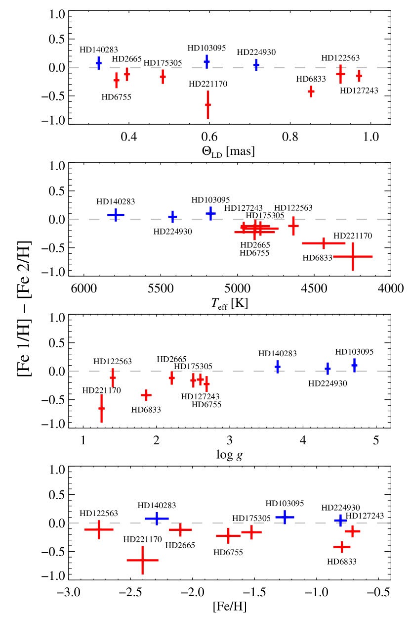
Figure 7: Deviations from ionization balance, i.e. the difference between the abundances determined from lines of neutral and ionized iron, as a function of the measured stellar parameters. Vertical and horizontal lines represent the combined uncertainties from the two measurements. Each star is labelled, and colour-coded as red for red giants or blue for main-sequence and subgiants.

5 Conclusions

This project delivered fundamental stellar parameters for ten metal-poor stars. Stars with low metallicity are poorly represented in benchmark sample used so far. Reliable angular diameters for metal poor stars have been difficult to measure so far because these stars are faint for suitable interferometric instruments. We took this into consideration, observed the stars over various nights, baseline configurations and tried to resolve the targets close to the first null of the visibility curve. We observed the stars using the high angular resolution instrument PAVO and the CHARA array and we measured accurate angular diameters of the stars.

In order to estimate the limb darkening diameters, we used the 3D radiation-hydrodynamical model atmospheres in the STAGGER-grid. The $T_{\mathrm{eff}}$ were directly computed from the Stefan-Boltzmann relation using the measured angular diameters and bolometric flux. Bolometric fluxes were computed from multi-band photometry interpolating iteratively on a grid of synthetic stellar fluxes, to ensure consistency with the final adopted stellar parameters. High resolution spectroscopy allowed us to determine $[\mathrm{Fe/H}]$, isochrone fitting to derive mass, and parallax measurements to constrain the absolute luminosity. After iterative refinement we derived the final fundamental parameters of $T_{\mathrm{eff}}$, $\log(g)$, $[\mathrm{Fe/H}]$.

This allowed us to reach the desired precision of better than 1% in the $T_{\mathrm{eff}}$ for 5 stars in our sample HD 103095, HD 122563, HD 127243, HD 140283 and HD 224930. A precision of 1% in $T_{\mathrm{eff}}$ is essential for the correct determination of the atmospheric parameters of the survey sources. For the remaining stars, for which the uncertainties in the $T_{\mathrm{eff}}$ are higher than 1%, the uncertainty in the bolometric flux significantly contributes to the final uncertainty in the effective temperature ($\sim$2-3%). For all stars in our sample we determined $\log(g)$ and $\mathrm{[Fe/H]}$, with median uncertainties of 0.03 dex and 0.09 dex, respectively.

We presented the first from the series of papers that are aiming to build a new robust sample of benchmark stars. The reliable interferometric stellar parameters presented here should be useful for testing and validating stellar analysis pipelines (Jofré et al., 2019), that typically rely on photometric and spectroscopic methods. Our consistent measurements and analysis will also help to cross-calibrate different large stellar surveys such as Gaia (Gaia Collaboration, 2018), APOGEE (Allende Prieto et al., 2008), Gaia-ESO Survey (Gilmore et al., 2012; Randich et al., 2013), 4MOST (de Jong et al., 2012), WEAVE (Dalton et al., 2012), GALAH (De Silva et al., 2015). In turn, achieving these goals will help us to more robustly understand the physics of stars, and uncover the structure and evolution of our Galaxy.