SALD: Sign Agnostic Learning with
Derivatives
Abstract
Learning 3D geometry directly from raw data, such as point clouds, triangle soups, or unoriented meshes is still a challenging task that feeds many downstream computer vision and graphics applications.
In this paper, we introduce SALD: a method for learning implicit neural representations of shapes directly from raw data. We generalize sign agnostic learning (SAL) to include derivatives: given an unsigned distance function to the input raw data, we advocate a novel sign agnostic regression loss, incorporating both pointwise values and gradients of the unsigned distance function. Optimizing this loss leads to a signed implicit function solution, the zero level set of which is a high quality and valid manifold approximation to the input 3D data. The motivation behind SALD is that incorporating derivatives in a regression loss leads to a lower sample complexity, and consequently better fitting. In addition, we prove that SAL enjoys a minimal length property in 2D, favoring minimal length solutions. More importantly, we are able to show that this property still holds for SALD, i.e., with derivatives included.
We demonstrate the efficacy of SALD for shape space learning on two challenging datasets: ShapeNet (Chang et al., 2015) that contains inconsistent orientation and non-manifold meshes, and D-Faust (Bogo et al., 2017) that contains raw 3D scans (triangle soups). On both these datasets, we present state-of-the-art results.
1 Introduction
Recently, neural networks (NN) have been used for representing and reconstructing 3D surfaces. Current NN-based 3D learning approaches differ in two aspects: the choice of surface representation, and the supervision method. Common representations of surfaces include using NN as parameteric charts of surfaces (Groueix et al., 2018b; Williams et al., 2019); volumetric implicit function representation defined over regular grids (Wu et al., 2016; Tatarchenko et al., 2017; Jiang et al., 2020); and NN used directly as volumetric implicit functions (Park et al., 2019; Mescheder et al., 2019; Atzmon et al., 2019; Chen & Zhang, 2019), referred henceforth as implicit neural representations. Supervision methods include regression of known or approximated volumetric implicit representations (Park et al., 2019; Mescheder et al., 2019; Chen & Zhang, 2019), regression directly with raw 3D data (Atzmon & Lipman, 2020; Gropp et al., 2020; Atzmon & Lipman, 2020), and differentiable rendering using 2D data (i.e., images) supervision (Niemeyer et al., 2020; Liu et al., 2019; Saito et al., 2019; Yariv et al., 2020).
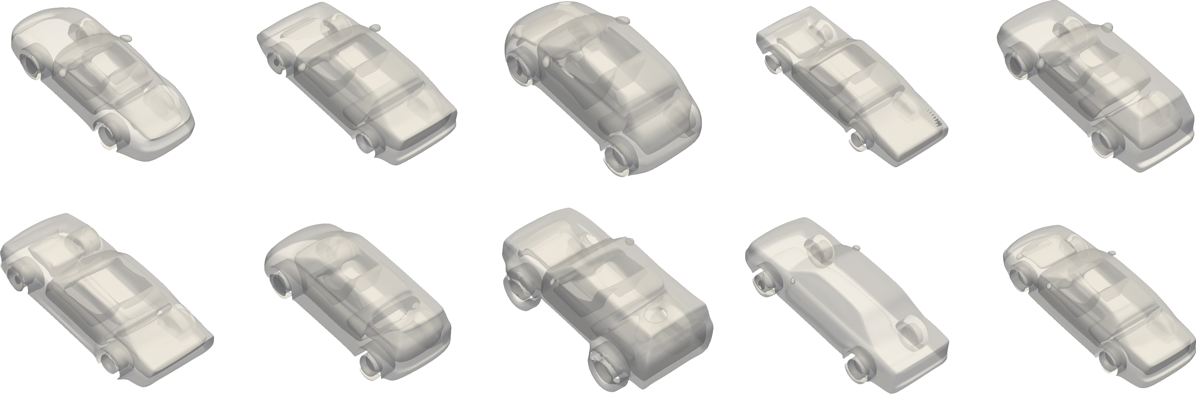
The goal of this paper is to introduce SALD, a method for learning implicit neural representations of surfaces directly from raw 3D data. The benefit in learning directly from raw data, e.g., non-oriented point clouds or triangle soups (e.g., Chang et al. (2015)) and raw scans (e.g., Bogo et al. (2017)), is avoiding the need for a ground truth signed distance representation of all train surfaces for supervision. This allows working with complex models with inconsistent normals and/or missing parts. In Figure 1 we show reconstructions of zero level sets of SALD learned implicit neural representations of car models from the ShapeNet dataset (Chang et al., 2015) with variational auto-encoder; notice the high detail level and the interior, which would not have been possible with, e.g., previous data pre-processing techniques using renderings of visible parts (Park et al., 2019).
Our approach improves upon the recent Sign Agnostic Learning (SAL) method (Atzmon & Lipman, 2020) and shows that incorporating derivatives in a sign agnostic manner provides a significant improvement in surface approximation and detail. SAL is based on the observation that given an unsigned distance function to some raw 3D data , a sign agnostic regression to will introduce new local minima that are signed versions of ; in turn, these signed distance functions can be used as implicit representations of the underlying surface. In this paper we show how the sign agnostic regression loss can be extended to compare both function values and derivatives , up to a sign.
The main motivation for performing NN regression with derivatives is that it reduces the sample complexity of the problem (Czarnecki et al., 2017), leading to better accuracy and generalization. For example, consider a one hidden layer NN of the form . Prescribing two function samples at are not sufficient for uniquely determining , while adding derivative information at these points determines uniquely.
Analyzing theoretical aspects of SAL and SALD, we observe that both possess the favorable minimal surface property, that is, in areas of missing parts and holes they will prefer zero level sets with minimal area. We justify this property by proving that, in 2D, when restricted to the zero level-set (a curve in this case), the SAL and SALD losses would encourage a straight line solution connecting neighboring data points.
We have tested SALD on the dataset of man-made models, ShapeNet (Chang et al., 2015), and human raw scan dataset, D-Faust (Bogo et al., 2017), and compared to state-of-the-art methods. In all cases we have used the raw input data as is and considered the unsigned distance function to , i.e., , in the SALD loss to produce an approximate signed distance function in the form of a neural network. Comparing to state-of-the-art methods we find that SALD achieves superior results on this dataset.
On the D-Faust dataset, when comparing to ground truth reconstructions we report state-of-the-art results, striking a balance between approximating details of the scans and avoiding overfitting noise and ghost geometry.
Summarizing the contributions of this paper:
-
Introducing sign agnostic learning with derivatives.
-
Identifying and providing a theoretical justification for the minimal surface property of sign agnostic learning.
-
Training directly on raw data (end-to-end) including unoriented or not consistently oriented triangle soups and raw 3D scans.
2 Previous work
Learning 3D shapes with neural networks and 3D supervision has shown great progress recently. We review related works, where we categorize the existing methods based on their choice of 3D surface representation.
Parametric representations. The most fundamental surface representation is an atlas, that is a collection of parametric charts with certain coverage and transition properties (Do Carmo, 2016). Groueix et al. (2018b) adapted this idea using neural network to represent a surface as union of such charts; Williams et al. (2019) improved this construction by introducing better transitions between charts; Sinha et al. (2016) use geometry images (Gu et al., 2002) to represent an entire shape using a single chart; Maron et al. (2017) use global conformal parameterization for learning surface data; Ben-Hamu et al. (2018) use a collection of overlapping global conformal charts for human-shape generative model. The benefit in parametric representations is in the ease of sampling the learned surface (i.e., forward pass) and work directly with raw data (e.g., Chamfer loss); their main struggle is in producing charts that are collectively consistent, of low distortion, and covering the shape.
Implicit representations. Another approach for representing surfaces is as zero level sets of a function, called an implicit function. There are two popular methods to model implicit volumetric functions with neural networks: i) Convolutional neural network predicting scalar values over a predefined fixed volumetric structure (e.g., grid or octree) in space (Tatarchenko et al., 2017; Wu et al., 2016); and ii) Multilayer Perceptron of the form defining a continuous volumetric function (Park et al., 2019; Mescheder et al., 2019; Chen & Zhang, 2019). Currently, neural networks are trained to be implicit function representations with two types of supervision: (i) regression of samples taken from a known or pre-computed implicit function representation such as occupancy function (Mescheder et al., 2019; Chen & Zhang, 2019) or a signed distance function (Park et al., 2019); and (ii) working with raw 3D supervision, by particle methods relating points on the level sets to the model parameters (Atzmon et al., 2019), using sign agnostic losses (Atzmon & Lipman, 2020), or supervision with PDEs defining signed distance functions (Gropp et al., 2020).
Primitives. Another type of representation is to learn shapes as composition or unions of a family of primitives. Li et al. (2019) represent a shape using a parametric collection of primitives. Genova et al. (2019; 2020) use a collection of Gaussians and learn consistent shape decompositions. Chen et al. (2020) suggest a differentiable Binary Space Partitioning tree (BSP-tree) for representing shapes. Deprelle et al. (2019) combine points and charts representations to learn basic shape structures. Deng et al. (2020) represent a shape as a union of convex sets. Williams et al. (2020) learn cites of Voronoi cells for implicit shape representation.
Template fitting. Lastly, several methods learn 3D shapes of a certain class (e.g., humans) by learning the deformation from a template model. Classical methods use matching techniques and geometric loss minimization for non-rigid template matching (Allen et al., 2002; 2003; Anguelov et al., 2005). Groueix et al. (2018a) use an auto-encoder architecture and Chamfer distance to match target shapes. Litany et al. (2018) use graph convolutional autoencoder to learn deformable template for shape completion.
3 Method
Given raw geometric input data , e.g., a triangle soup, our goal is to find a multilayer perceptron (MLP) whose zero level-set,
| (1) |
is a manifold surface that approximates .
Sign agnostic learning. Similarly to SAL, our approach is to consider the (readily available) unsigned distance function to the raw input geometry,
| (2) |
and perform sign agnostic regression to get a signed version of . SAL uses a loss of the form
| (3) |
where is some probability distribution, and is an unsigned similarity. That is, is measuring the difference between scalars up-to a sign. For example
| (4) |
is an example that is used in Atzmon & Lipman (2020). The key property of the sign agnostic loss in equation 3 is that, with proper weights initialization , it finds a new signed local minimum which in absolute value is similar to . In turn, the zero level set of is a valid manifold describing the data .
Sign agnostic learning with derivatives. Our goal is to generalize the SAL loss (equation 3) to include derivative data of and show that optimizing this loss provides implicit neural representations, , that enjoy better approximation properties with respect to the underlying geometry .
Generalizing equation 3 requires designing an unsigned similarity measure for vector valued functions. The key observation is that equation 4 can be written as , , and can be generalized to vectors by
| (5) |
We define the SALD loss:
| (6) |
where is a parameter, is a probability distribution, and are the gradients (resp.) with respect to their input .
 |
 |
 |
| unsigned distance | SALD | SAL |
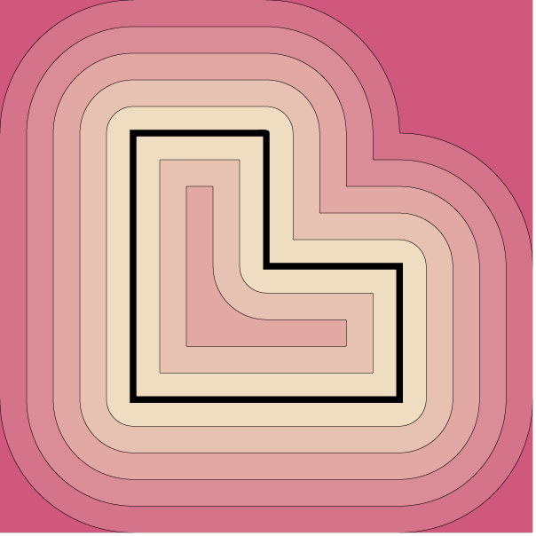
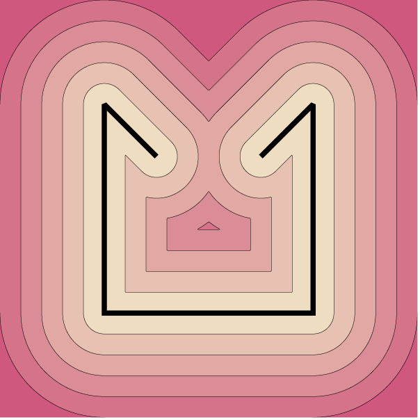
In Figure 2 we show the unsigned distance to an L-shaped curve (left), and the level sets of the MLPs optimized with the SALD loss (middle) and the SAL loss (right); note that SALD loss reconstructed the sharp features (i.e., corners) of the shape and the level sets of , while SAL loss smoothed them out; the implementation details of this experiment can be found in Appendix A.4.
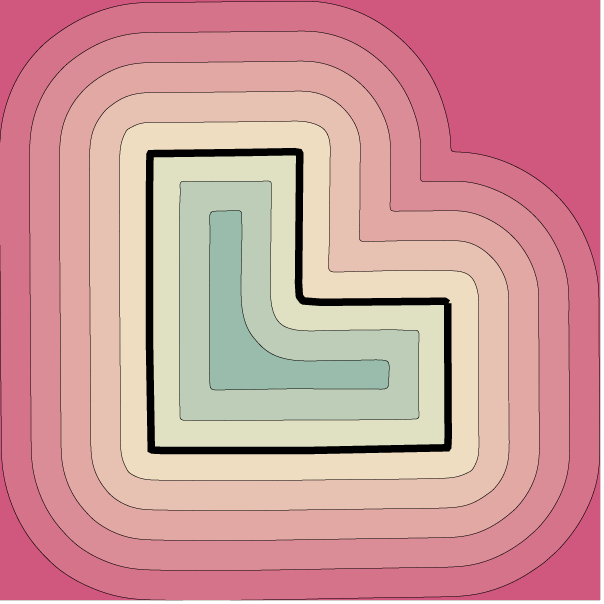
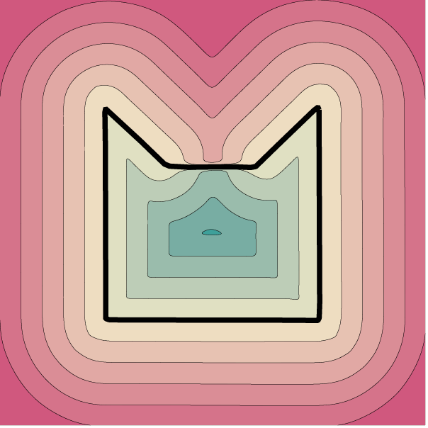
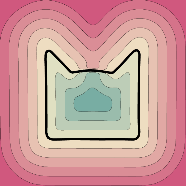
Minimal surface property. We show that the SAL and SALD losses possess a minimal surface property (Zhao et al., 2001), that is, they strives to minimize surface area of missing parts. For example, Figure 4 shows the unsigned distance to a curve with a missing segment (left), and the zero level sets of MLPs optimized with SALD loss (middle), and SAL loss (right). Note that in both cases the zero level set in the missing part area is the minimal length curve (i.e., a line) connecting the end points of that missing part. SALD also preserves sharp features of the rest of the shape.
We will provide a theoretical justification to this property in the 2D case. We consider a geometry defined by two points in the plane, and possible solutions where the zero level set curve is connecting and . We prove that among a class of curves connecting and , the straight line minimizes the losses in equation 3 and equation 6 restricted to , when assuming uniform distributions .
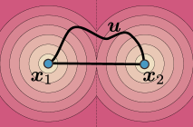
We assume (without losing generality) that , and consider curves defined by , where , and is some differentiable function such that , see Figure 3.
For the SALD loss we prove the claim for a slightly simplified agnostic loss motivated by the following lemma proved in Appendix A.1:
Lemma 1.
For any pair of unit vectors : .
We consider for the derivative part of the loss in equation 6, which is also sign agnostic.
Theorem 1.
Proof.
The unsigned distance function is
From symmetry it is enough to consider only the first half of the curve, i.e., . Then, the SAL loss, equation 3, restricted to the curve (i.e., where vanishes) takes the form
where is the length element on the curve , and , since over the curve . Plugging in we see that the curve , namely the straight line curve from to is a strict global minimizer of . Similar argument on prove the claim for the SAL case.
 |
 |
 |
| unsigned distance | SALD | SAL |
For the SALD case, we want to calculate restricted to the curve ; let and . First, . Second, is normal to the curve , therefore it is proportional to . Next, note that
where the last equality can be checked by differentiating w.r.t. . Therefore,
This bound is achieved for the curve , which is also a minimizer of the SAL loss. The straight line also minimizes this version of the SALD loss since ∎
4 Experiments
We tested SALD on the task of shape space learning from raw 3D data. We experimented with two different datasets: i) ShapeNet dataset (Chang et al., 2015), containing synthetic 3D Meshes; and ii) D-Faust dataset (Bogo et al., 2017) containing raw 3D scans.
Shape space learning architecture. Our method can be easily incorporated into existing shape space learning architectures: i) Auto-Decoder (AD) suggested in Park et al. (2019); and the ii) Modified Variational Auto-Encoder (VAE) used in Atzmon & Lipman (2020). For VAE, the encoder is taken to be PointNet (Qi et al., 2017). For both options, the decoder is the implicit representation in equation 1, where is taken to be an 8-layer MLP with 512 hidden units in each layer and Softplus activation. In addition, to enable sign agnostic learning we initialize the decoder weights, , using the geometric initialization from Atzmon & Lipman (2020). See Appendix A.2.3 for more details regarding the architecture.
Baselines. The baseline methods selected for comparison cover both existing supervision methodologies: DeepSDF (Park et al., 2019) is chosen as a representative out of the methods that require pre-computed implicit representation for training. For methods that train directly on raw 3D data, we compare versus SAL (Atzmon & Lipman, 2020) and IGR (Gropp et al., 2020). See Appendix A.5 for a detailed description of the quantitative metrics used for evaluation.
| Category | Sofas | Chairs | Tables | Planes | Lamps | |||||
|---|---|---|---|---|---|---|---|---|---|---|
| Mean | Median | Mean | Median | Mean | Median | Mean | Median | Mean | Median | |
| DeepSDF | 0.329 | 0.230 | 0.341 | 0.133 | 0.839 | 0.149 | 0.177 | 0.076 | 0.909 | 0.344 |
| SAL | 0.704 | 0.523 | 0.494 | 0.259 | 0.543 | 0.231 | 0.429 | 0.146 | 4.913 | 1.515 |
| SALD(VAE) | 0.391 | 0.244 | 0.415 | 0.255 | 0.679 | 0.279 | 0.197 | 0.062 | 1.808 | 1.172 |
| SALD(AD) | 0.207 | 0.147 | 0.281 | 0.157 | 0.408 | 0.25 | 0.098 | 0.032 | 0.506 | 0.327 |
4.1 ShapeNet
In this experiment we tested SALD ability to learn a shape space by training on a challenging 3D data such as non-manifold/non-orientable meshes. We tested SALD with both AD and VAE architectures. In both settings, we set for the SALD loss. We follow the evaluation protocol as in Park et al. (2019): using the same train/test splits, we train and evaluate our method on different categories. Note that comparison versus IGR is omitted as IGR requires consistently oriented normals for shape space learning, which is not available for ShapeNet, where many models have non-consistent triangles’ orientation.
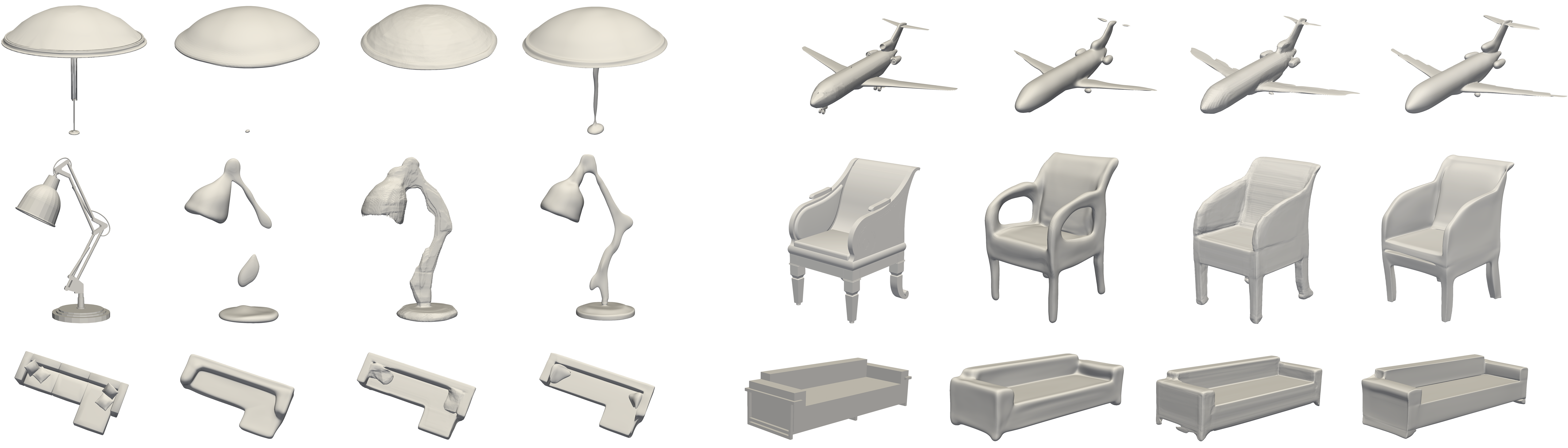
Results. Table 1 and Figure 5 show quantitative and qualitative results (resp.) for the held-out test set, comparing SAL, DeepSDF and SALD. As can be read from the table and inspected in the figure, our method, when used with the same auto-decoder as in DeepSDF, compares favorably to DeepSDF’s reconstruction performance on this data.
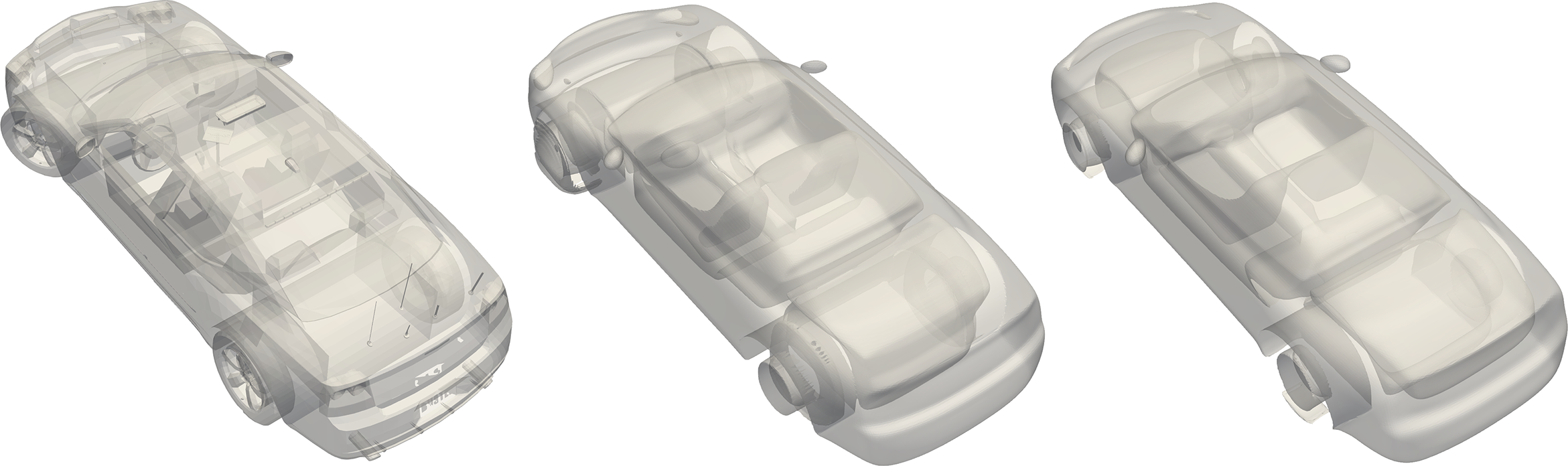
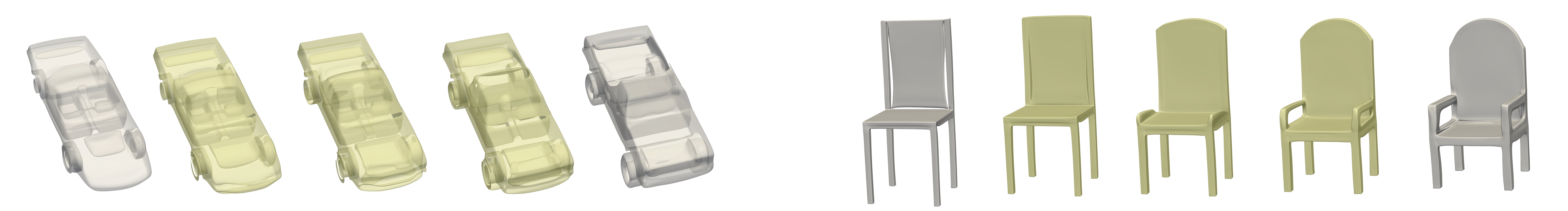
Qualitatively the surfaces produces by SALD are smoother, mostly with more accurate sharp features, than SAL and DeepSDF generated surfaces. Figure 1 shows typical train and test results from the Cars class with VAE. Figure 6 shows a comparison between SALD shape space learning with VAE and AD in reconstruction of a test car model (left). Note that the AD (middle) seems to produce more details of the test model than the VAE (right), e.g., steering wheel and headlights. Figure 7 show SALD (AD) generated shapes via latent space interpolation between two test models.
4.2 D-Faust
The D-Faust dataset (Bogo et al., 2017) contains raw scans (triangle soups) of 10 humans in multiple poses. There are approximately 41k scans in the dataset. Due to the low variety between adjacent scans, we sample each pose scans at a ratio of . The leftmost column in Figure 8 shows examples of raw scans used for training. For evaluation we use the registrations provided with the data set. Note that the registrations where not used for training. We tested SALD using the VAE architecture, with set for the SALD loss. We followed the evaluation protocol as in Atzmon & Lipman (2020), using the same train/test split. Note that Atzmon & Lipman (2020) already conducted a comprehensive comparison of SAL versus DeepSDF, establishing SAL as a state-of-the-art method for this dataset. Thus, we focus on comparison versus SAL and IGR.
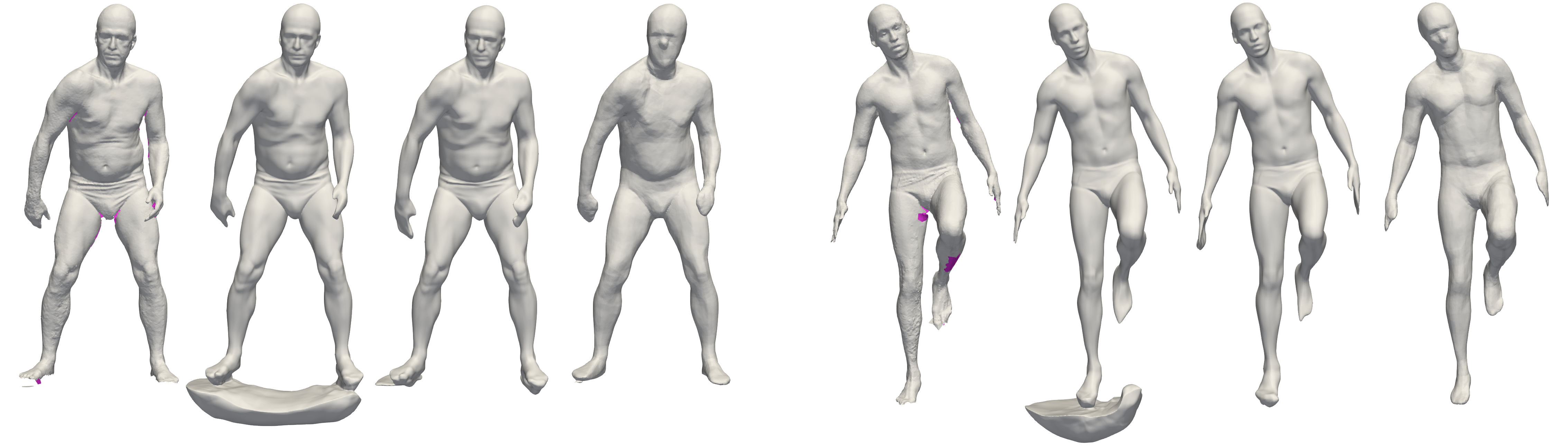
Results. Table 2 and Figure 8 show quantitative and qualitative results (resp.); although SALD does not produces the best test quantitative results, it is roughly comparable in every measure to the best among the two baselines. That is, it produces details comparable to IGR while maintaining the minimal surface property as SAL and not adding undesired surface sheets as IGR; see the figure for visual illustrations of these properties: the high level of details of SALD and IGR compared to SAL, and the extraneous parts added by IGR, avoided by SALD. These phenomena can also be seen quantitatively, e.g., the reconstruction-to-registration loss of IGR. Figure 9 show SALD generated shapes via latent space interpolation between two test scans. Notice the ability of SALD to generate novel mixed faces and body parts.
| Mean | Median | Mean | Median | Mean | Median | Mean | Median | Mean | Median | Mean | Median | |
|---|---|---|---|---|---|---|---|---|---|---|---|---|
| SAL | 0.418 | 0.328 | 13.21 | 12.459 | 0.344 | 0.256 | 11.354 | 10.522 | 0.429 | 0.246 | 10.096 | 9.096 |
| IGR | 0.276 | 0.187 | 10.328 | 9.822 | 3.806 | 3.627 | 17.124 | 17.902 | 0.241 | 0.11 | 5.829 | 5.295 |
| SALD | 0.428 | 0.346 | 11.67 | 11.07 | 0.489 | 0.362 | 11.035 | 10.371 | 0.397 | 0.279 | 7.884 | 7.227 |
4.3 Limitations
Figure 10 shows typical failure cases of our method from the ShapeNet experiment described above.
We mainly suffer from two types of failures: First, since inside and outside information is not known (and often not even well defined in ShapeNet models) SALD can add surface sheets closing what should be open areas (e.g., the bottom side of the lamp, or holes in the chair). Second, thin structures can be missed (e.g., the electric cord of the lamp on the left).
5 Conclusions
We introduced SALD, a method for learning implicit neural representations from raw data. The method is based on a generalization of the sign agnostic learning idea to include derivative data. We demonstrated that the addition of a sign agnostic derivative term to the loss improves the approximation power of the resulting signed implicit neural network. In particular, showing improvement in the level of details and sharp features of the reconstructions. Furthermore, we identify the favorable minimal surface property of the SAL and SALD losses and provide a theoretical justification in 2D. Generalizing this analysis to 3D is marked as interesting future work.
We see two more possible venues for future work: First, it is clear that there is room for further improvement in approximation properties of implicit neural representations. Although the results in D-Faust are already close to the input quality, in ShapeNet we still see a gap between input models and their implicit neural representations; this challenge already exists in overfitting a large collection of diverse shapes in the training stage. Improvement can come from adding expressive power to the neural networks, or further improving the training losses; adding derivatives as done in this paper is one step in that direction but does not solves the problem completely. Combining sign agnostic learning with the recent positional encoding method (Tancik et al., 2020) could also be an interesting future research venue. Second, it is interesting to think of applications or settings in which SALD can improve the current state-of-the-art. Generative 3D modeling is one concrete option, learning geometry with 2D supervision is another.
References
- Allen et al. (2002) Brett Allen, Brian Curless, and Zoran Popović. Articulated body deformation from range scan data. ACM Transactions on Graphics (TOG), 21(3):612–619, 2002.
- Allen et al. (2003) Brett Allen, Brian Curless, and Zoran Popović. The space of human body shapes: reconstruction and parameterization from range scans. ACM transactions on graphics (TOG), 22(3):587–594, 2003.
- Anguelov et al. (2005) Dragomir Anguelov, Praveen Srinivasan, Daphne Koller, Sebastian Thrun, Jim Rodgers, and James Davis. Scape: shape completion and animation of people. In ACM SIGGRAPH 2005 Papers, pp. 408–416. 2005.
- Atzmon & Lipman (2020) Matan Atzmon and Yaron Lipman. Sal: Sign agnostic learning of shapes from raw data. In IEEE/CVF Conference on Computer Vision and Pattern Recognition (CVPR), June 2020.
- Atzmon et al. (2019) Matan Atzmon, Niv Haim, Lior Yariv, Ofer Israelov, Haggai Maron, and Yaron Lipman. Controlling neural level sets. In Advances in Neural Information Processing Systems, pp. 2032–2041, 2019.
- Baydin et al. (2017) Atılım Günes Baydin, Barak A Pearlmutter, Alexey Andreyevich Radul, and Jeffrey Mark Siskind. Automatic differentiation in machine learning: a survey. The Journal of Machine Learning Research, 18(1):5595–5637, 2017.
- Ben-Hamu et al. (2018) Heli Ben-Hamu, Haggai Maron, Itay Kezurer, Gal Avineri, and Yaron Lipman. Multi-chart generative surface modeling. ACM Transactions on Graphics (TOG), 37(6):1–15, 2018.
- Bogo et al. (2017) Federica Bogo, Javier Romero, Gerard Pons-Moll, and Michael J Black. Dynamic faust: Registering human bodies in motion. In Proceedings of the IEEE conference on computer vision and pattern recognition, pp. 6233–6242, 2017.
- Chang et al. (2015) Angel X Chang, Thomas Funkhouser, Leonidas Guibas, Pat Hanrahan, Qixing Huang, Zimo Li, Silvio Savarese, Manolis Savva, Shuran Song, Hao Su, et al. Shapenet: An information-rich 3d model repository. arXiv preprint arXiv:1512.03012, 2015.
- Chen & Zhang (2019) Zhiqin Chen and Hao Zhang. Learning implicit fields for generative shape modeling. In Proceedings of the IEEE Conference on Computer Vision and Pattern Recognition, pp. 5939–5948, 2019.
- Chen et al. (2020) Zhiqin Chen, Andrea Tagliasacchi, and Hao Zhang. Bsp-net: Generating compact meshes via binary space partitioning. Proceedings of IEEE Conference on Computer Vision and Pattern Recognition (CVPR), 2020.
- Czarnecki et al. (2017) Wojciech M Czarnecki, Simon Osindero, Max Jaderberg, Grzegorz Swirszcz, and Razvan Pascanu. Sobolev training for neural networks. In Advances in Neural Information Processing Systems, pp. 4278–4287, 2017.
- Deng et al. (2020) Boyang Deng, Kyle Genova, Soroosh Yazdani, Sofien Bouaziz, Geoffrey Hinton, and Andrea Tagliasacchi. Cvxnet: Learnable convex decomposition. June 2020.
- Deprelle et al. (2019) Theo Deprelle, Thibault Groueix, Matthew Fisher, Vladimir Kim, Bryan Russell, and Mathieu Aubry. Learning elementary structures for 3d shape generation and matching. In Advances in Neural Information Processing Systems, pp. 7433–7443, 2019.
- Do Carmo (2016) Manfredo P Do Carmo. Differential Geometry of Curves and Surfaces: Revised and Updated Second Edition. Courier Dover Publications, 2016.
- Genova et al. (2019) Kyle Genova, Forrester Cole, Daniel Vlasic, Aaron Sarna, William T Freeman, and Thomas Funkhouser. Learning shape templates with structured implicit functions. In Proceedings of the IEEE International Conference on Computer Vision, pp. 7154–7164, 2019.
- Genova et al. (2020) Kyle Genova, Forrester Cole, Avneesh Sud, Aaron Sarna, and Thomas Funkhouser. Local deep implicit functions for 3d shape. In Proceedings of the IEEE/CVF Conference on Computer Vision and Pattern Recognition, pp. 4857–4866, 2020.
- Gropp et al. (2020) Amos Gropp, Lior Yariv, Niv Haim, Matan Atzmon, and Yaron Lipman. Implicit geometric regularization for learning shapes. In Proceedings of Machine Learning and Systems 2020, 2020.
- Groueix et al. (2018a) Thibault Groueix, Matthew Fisher, Vladimir G Kim, Bryan C Russell, and Mathieu Aubry. 3d-coded: 3d correspondences by deep deformation. In Proceedings of the European Conference on Computer Vision (ECCV), pp. 230–246, 2018a.
- Groueix et al. (2018b) Thibault Groueix, Matthew Fisher, Vladimir G Kim, Bryan C Russell, and Mathieu Aubry. A papier-mâché approach to learning 3d surface generation. In Proceedings of the IEEE conference on computer vision and pattern recognition, pp. 216–224, 2018b.
- Gu et al. (2002) Xianfeng Gu, Steven J Gortler, and Hugues Hoppe. Geometry images. In Proceedings of the 29th annual conference on Computer graphics and interactive techniques, pp. 355–361, 2002.
- Jiang et al. (2020) Yue Jiang, Dantong Ji, Zhizhong Han, and Matthias Zwicker. Sdfdiff: Differentiable rendering of signed distance fields for 3d shape optimization. In Proceedings of the IEEE/CVF Conference on Computer Vision and Pattern Recognition, pp. 1251–1261, 2020.
- Kingma & Ba (2014) Diederik P Kingma and Jimmy Ba. Adam: A method for stochastic optimization. arXiv preprint arXiv:1412.6980, 2014.
- Li et al. (2019) Lingxiao Li, Minhyuk Sung, Anastasia Dubrovina, Li Yi, and Leonidas J Guibas. Supervised fitting of geometric primitives to 3d point clouds. In Proceedings of the IEEE Conference on Computer Vision and Pattern Recognition, pp. 2652–2660, 2019.
- Litany et al. (2018) Or Litany, Alex Bronstein, Michael Bronstein, and Ameesh Makadia. Deformable shape completion with graph convolutional autoencoders. In Proceedings of the IEEE conference on computer vision and pattern recognition, pp. 1886–1895, 2018.
- Liu et al. (2019) Shichen Liu, Shunsuke Saito, Weikai Chen, and Hao Li. Learning to infer implicit surfaces without 3d supervision. In Advances in Neural Information Processing Systems, pp. 8293–8304, 2019.
- Lorensen & Cline (1987) William E Lorensen and Harvey E Cline. Marching cubes: A high resolution 3d surface construction algorithm. In ACM siggraph computer graphics, volume 21, pp. 163–169. ACM, 1987.
- Maron et al. (2017) Haggai Maron, Meirav Galun, Noam Aigerman, Miri Trope, Nadav Dym, Ersin Yumer, Vladimir G Kim, and Yaron Lipman. Convolutional neural networks on surfaces via seamless toric covers. ACM Trans. Graph., 36(4):71–1, 2017.
- Mescheder et al. (2019) Lars Mescheder, Michael Oechsle, Michael Niemeyer, Sebastian Nowozin, and Andreas Geiger. Occupancy networks: Learning 3d reconstruction in function space. In Proceedings of the IEEE Conference on Computer Vision and Pattern Recognition, pp. 4460–4470, 2019.
- Niemeyer et al. (2020) Michael Niemeyer, Lars Mescheder, Michael Oechsle, and Andreas Geiger. Differentiable volumetric rendering: Learning implicit 3d representations without 3d supervision. In Proceedings of the IEEE/CVF Conference on Computer Vision and Pattern Recognition, pp. 3504–3515, 2020.
- Park et al. (2019) Jeong Joon Park, Peter Florence, Julian Straub, Richard Newcombe, and Steven Lovegrove. Deepsdf: Learning continuous signed distance functions for shape representation. In The IEEE Conference on Computer Vision and Pattern Recognition (CVPR), June 2019.
- Paszke et al. (2017) Adam Paszke, Sam Gross, Soumith Chintala, Gregory Chanan, Edward Yang, Zachary DeVito, Zeming Lin, Alban Desmaison, Luca Antiga, and Adam Lerer. Automatic differentiation in pytorch. 2017.
- Qi et al. (2017) Charles R Qi, Hao Su, Kaichun Mo, and Leonidas J Guibas. Pointnet: Deep learning on point sets for 3d classification and segmentation. In Proceedings of the IEEE Conference on Computer Vision and Pattern Recognition, pp. 652–660, 2017.
- Saito et al. (2019) Shunsuke Saito, Zeng Huang, Ryota Natsume, Shigeo Morishima, Angjoo Kanazawa, and Hao Li. Pifu: Pixel-aligned implicit function for high-resolution clothed human digitization. In Proceedings of the IEEE International Conference on Computer Vision, pp. 2304–2314, 2019.
- Sinha et al. (2016) Ayan Sinha, Jing Bai, and Karthik Ramani. Deep learning 3d shape surfaces using geometry images. In European Conference on Computer Vision, pp. 223–240. Springer, 2016.
- Tancik et al. (2020) Matthew Tancik, Pratul P. Srinivasan, Ben Mildenhall, Sara Fridovich-Keil, Nithin Raghavan, Utkarsh Singhal, Ravi Ramamoorthi, Jonathan T. Barron, and Ren Ng. Fourier features let networks learn high frequency functions in low dimensional domains. NeurIPS, 2020.
- Tatarchenko et al. (2017) Maxim Tatarchenko, Alexey Dosovitskiy, and Thomas Brox. Octree generating networks: Efficient convolutional architectures for high-resolution 3d outputs. In Proceedings of the IEEE International Conference on Computer Vision, pp. 2088–2096, 2017.
- The CGAL Project (2020) The CGAL Project. CGAL User and Reference Manual. CGAL Editorial Board, 5.0.2 edition, 2020. URL https://doc.cgal.org/5.0.2/Manual/packages.html.
- Williams et al. (2019) Francis Williams, Teseo Schneider, Claudio Silva, Denis Zorin, Joan Bruna, and Daniele Panozzo. Deep geometric prior for surface reconstruction. In Proceedings of the IEEE Conference on Computer Vision and Pattern Recognition, pp. 10130–10139, 2019.
- Williams et al. (2020) Francis Williams, Jerome Parent-Levesque, Derek Nowrouzezahrai, Daniele Panozzo, Kwang Moo Yi, and Andrea Tagliasacchi. Voronoinet: General functional approximators with local support. In Proceedings of the IEEE/CVF Conference on Computer Vision and Pattern Recognition Workshops, pp. 264–265, 2020.
- Wu et al. (2016) Jiajun Wu, Chengkai Zhang, Tianfan Xue, Bill Freeman, and Josh Tenenbaum. Learning a probabilistic latent space of object shapes via 3d generative-adversarial modeling. In Advances in neural information processing systems, pp. 82–90, 2016.
- Yariv et al. (2020) Lior Yariv, Yoni Kasten, Dror Moran, Meirav Galun, Matan Atzmon, Ronen Basri, and Yaron Lipman. Multiview neural surface reconstruction with implicit lighting and material. arXiv preprint arXiv:2003.09852, 2020.
- Zaheer et al. (2017) Manzil Zaheer, Satwik Kottur, Siamak Ravanbakhsh, Barnabas Poczos, Ruslan R Salakhutdinov, and Alexander J Smola. Deep sets. In Advances in neural information processing systems, pp. 3391–3401, 2017.
- Zhao et al. (2001) Hong-Kai Zhao, Stanley Osher, and Ronald Fedkiw. Fast surface reconstruction using the level set method. In Proceedings IEEE Workshop on Variational and Level Set Methods in Computer Vision, pp. 194–201. IEEE, 2001.
Appendix A Appendix
A.1 Proof of Lemma 1
Lemma 1.
For any pair of unit vectors : .
Proof.
Let be arbitrary unit norm vectors. Then,
Where the last inequality can be proved by considering two cases: and , where we denote . In the first case , and in this case . The inequality is proved by considering
for . For the case we have . This case is proved by considering
for ∎
A.2 Implementation Details
A.2.1 Data Preparation
Given some raw 3D data , SALD loss (See equation 6) is computed on points and corresponding unsigned distance derivatives, and (resp.) sampled from some distributions and . In this paper, we set , where is chosen by uniform sampling points from and placing two isotropic Gaussians, and for each . The distribution parameter depends on each point , set to be as the distance of the \nth50 closest point to , whereas is set to fixed. is chosen by projecting to . The distribution is set to uniform on ; note that on , is a sub-differential which is the convex hull of the two possible normal vectors () at ; as the sign-agnostic loss does not differ between the two normal choices, we arbitrarily use one of them in the loss. Computing the unsigned distance to is done using the CGAL library (The CGAL Project, 2020). To speed up training, we precomputed for each shape in the dataset, 500K samples of the form and .
A.2.2 Gradient computation
The SALD loss requires incorporating the term in a differentiable manner. Our computation of is based on Automatic Differentiation (Baydin et al., 2017) forward mode. Similarly to Gropp et al. (2020), is constructed as a network consists of layers of the form
where denotes the output of the layer in and are the learnable parameters.
A.2.3 Architecture Details
VAE Architecture
Our VAE architecture is based on the one used in Atzmon & Lipman (2020). The encoder , where is the input point cloud, is composed of DeepSets (Zaheer et al., 2017) and PointNet (Qi et al., 2017) layers. Each layer consists of
where is the concat operation, and are the layer weights and bias and is the pointwise non-linear ReLU activation function. Our encoder architecture is:
where denotes a fully connected layer. The final two fully connected layers outputs vectors and used for parametrization of a multiviariate Gaussian used for sampling a latent vector . Our encoder architecture is similar to the one used in Mescheder et al. (2019).
Our decoder is a composition of layers where the first layer is , middle layers are and the final layer is . Notice that the input for the decoder is where and is the latent vector. In addition, we add a skip connection between the input to the middle fourth layer. We chose the Softplus with for the non linear activation in the layers. For regulrization of the latent , we add the following term to training loss
similarly to Atzmon & Lipman (2020).
Auto-Decoder Architecture
We use an auto-decoder architecture, similar to the one suggested in Park et al. (2019). We defined the latent vector . The decoder architecture is the same as the one described above for the VAE. For regulrization of the latent , we add the following term to the loss
similarly to Park et al. (2019).
A.3 Training details
We trained our networks using the Adam (Kingma & Ba, 2014) optimizer, setting the batch size to . On each training step the SALD loss is evaluated on a random draw of points out of the precomputed 500K samples. For the VAE, we set a fixed learning rate of , whereas for the AD we scheduled the learning rate to start from and decrease by a factor of every epochs. All models were trained for epochs. Training was done on Nvidia V-100 GPUs, using pytorch deep learning framework (Paszke et al., 2017).
A.4 Figures 2 and 4
For the two dimensional experiments in figures 2 and 4 we have used the same decoder as in the VAE architecture with the only difference that the first layer is (no concatenation of a latent vector to the 2D input). We optimized using the Adam (Kingma & Ba, 2014) optimizer, for epochs. The parameter in the SALD loss was set to .
A.5 Evaluation
Evaluation metrics.
We use the following Chamfer distance metrics to measure similarity between shapes:
| (7) |
where
| (8) |
and the sets are either point clouds or triangle soups. In addition, to measure similarity of the normals of triangle soups , we define:
| (9) |
where
| (10) |
where is the positive angle between vectors , denotes the face normal of a point in triangle soup , and is the projection of on .
Tables 1 and 2 in the main paper report quantitative evaluation of our method, compared to other baselines. The meshing of the learned implicit representation was done using the Marching Cubes algorithm (Lorensen & Cline, 1987) on a uniform cubical grid of size . Computing the evaluation metrics and is done on a uniform sample of K points from the meshed surface.