A $t$-distribution based operator for enhancing
out of distribution robustness of neural network classifiers

Abstract

Neural Network (NN) classifiers can assign extreme probabilities to samples that have not appeared during training (out-of-distribution samples) resulting in erroneous and unreliable predictions. One of the causes for this unwanted behaviour lies in the use of the standard softmax operator which pushes the posterior probabilities to be either zero or unity hence failing to model uncertainty. The statistical derivation of the softmax operator relies on the assumption that the distributions of the latent variables for a given class are Gaussian with known variance. However, it is possible to use different assumptions in the same derivation and attain from other families of distributions as well. This allows derivation of novel operators with more favourable properties. Here, a novel operator is proposed that is derived using $t$-distributions which are capable of providing a better description of uncertainty. It is shown that classifiers that adopt this novel operator can be more robust to out of distribution samples, often outperforming NNs that use the standard softmax operator. These enhancements can be reached with minimal changes to the NN architecture.

I Introduction

Numerous scientific fields have found in deep learning efficient tools for classification. When enough labelled data is available a neural network (NN) is nowadays the most popular choice and often represents the state-of-the-art. Many signal processing tasks have recently adopted NN classifiers as well, for example in computer vision [1], audio processing [2, 3, 4] and speech recognition [5, 6]. Despite their popularity, NN classifiers can sometimes completely fail in their predictions, assigning high confidence to out-of-distribution (OOD) samples [7]. This problematic behaviour has been addressed in a number of recent studies where different solutions have been proposed.

A direct solution to this issue is train classifiers augmenting the training set with OOD samples. It has been shown that this exposure generalizes well to unmodeled distributions [8, 9]. These OOD datasets can also be obtained by synthesising adversarial samples [9, 10]. However, there can never be the certainty that these OOD datasets are representative of all the possible OOD samples that might be present in real case scenarios. Moreover, these procedures can substantially increase the training time and often require additional tuning of hyperparameters. Obtaining reliable classifiers without the need of employing OOD datasets is therefore attractive. This can be achieved by developing robust confidence measures that can indicate whether the classifier is wrong. The simplest confidence measure that can be obtained without any modification of the NN architecture consists of the softmax output [11], although we argue that this can often be unsatisfactory. More trustworthy confidence measures can be produced through Monte Carlo methods for example by employing dropout during the forward pass [12]. Alternatively, confidence measures can be obtained by combining the outputs of an ensemble of classifiers [13]. However, these approaches are rather computationally demanding. More recently OOD identification has been achieved by a temperature scaling of the softmax operator combined with a perturbation of the input sample [14]. This perturbation is obtained through differentiation and can also be considered costly for certain applications. Other techniques rely on learning confidence measures using particular cost functions and appending to NNs architecture an additional output branch that provides a score of reliability [15, 16].

In this paper a novel method that produces reliable confidence measures is proposed. This does not require the need of any OOD distribution dataset, avoids any substantial increase of the computational complexity and works with standard training procedures. The key idea is to replace the softmax operator of NNs with a different operator that inherently promotes low confidence for OOD samples. This operator is obtained by a modification of the statistical derivation of the softmax operator that amounts to using $t$-distributions instead of Gaussians to model the probability of latent variables for a given class. For this reason the proposed operator is named $t$-softmax. This idea can be traced back at least to [17] where it is shown that posterior probabilities obtained using $t$-distributions instead of Gaussian distributions can avoid high confidence predictions in regions where data is not available. Variations of the softmax operator have already appeared but for other purposes such as enhanced embeddings clustering [18, 19] and for reinforcement learning [20].

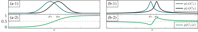
Figure 1: Sigmoid function (a-2) and $t$-sigmoid function (b-2) can be derived as posterior probabilities $p(C_{i}|x)$. The conditional distributions used to model the distribution for the latent variable $x$ are either Gaussian distributions (a-1) or $t$-distributions with $\nu=1$ (b-1).

II Statistical derivation of the softmax operator

The statistical derivation of the softmax operator can be found in [21] and is summarized in this section. Bayes’s theorem can be used to express the probability of a sample $\mathbf{x}\in\mathds{R}^{N}$ from a random latent variable belonging to the class $i$ as:

$$P(C_{i}|\mathbf{x})=\frac{p(\mathbf{x}|C_{i})P(C_{i})}{\sum_{i=1}^{N_{c}}p(\mathbf{x}|C_{i})P(C_{i})},$$ (1)

where $N_{c}$ is the number of classes and $C_{i}$ and $\mathbf{x}$ refer to the events that $C=i$ and the sample takes value $\mathbf{x}$, respectively. It is assumed that $p(\mathbf{x}|C_{i})$ is a Gaussian distribution with mean $\boldsymbol{\mu}_{i}\in\mathds{R}^{N}$ and covariance matrix $\boldsymbol{\Sigma}_{i}\in\mathds{R}^{N\times N}$:

$$p(\mathbf{x}|C_{i})=\tfrac{1}{\sqrt{(2\pi)^{N}|\boldsymbol{\Sigma}_{i}|}}\exp\left(-\tfrac{1}{2}(\mathbf{x}+\boldsymbol{\mu}_{i})^{\intercal}\boldsymbol{\Sigma}^{-1}_{i}(\mathbf{x}+\boldsymbol{\mu}_{i})\right),$$ (2)

for $i=1,\dots,N_{c}$. Furthermore, it is assumed that the prior probabilities are all equal ifnextchar,i.e.i.e.,  $P(C_{1})=P(C_{2})=\dots=P(C_{N_{c}})$ and that all Gaussian distributions share the same covariance matrix ifnextchar,i.e.i.e., $\boldsymbol{\Sigma}_{1}=\dots=\boldsymbol{\Sigma}_{N_{c}}=\boldsymbol{\Sigma}$. Under these assumptions, substituting (2) into (1) the softmax operator can be obtained:

$$P(C_{i}|\mathbf{x})=\frac{\exp\left(-\tfrac{1}{2}\left(a+\mathbf{w}_{i}^{\intercal}\mathbf{x}+b_{i}\right)\right)}{\sum_{k=1}^{N_{c}}\exp\left(-\tfrac{1}{2}\left(a+\mathbf{w}_{k}^{\intercal}\mathbf{x}+b_{k}\right)\right)}$$ (3)

where:

$$a=\mathbf{x}^{\intercal}\boldsymbol{\Sigma}^{-1}\mathbf{x},$$ (4)

is a constant that vanishes and

$$\mathbf{w}_{i}=2\boldsymbol{\Sigma}^{-1}\boldsymbol{\mu}_{i},$$ (5)

can be interpreted as the weights and

$$b_{i}=\boldsymbol{\mu}_{i}^{\intercal}\boldsymbol{\Sigma}^{-1}\boldsymbol{\mu}_{i},$$ (6)

as the biases of a fully connected layer $\mathbf{W}\mathbf{x}+\mathbf{b}$ with $\mathbf{W}=[\mathbf{w}_{1};\dots;\mathbf{w}_{N_{c}}]\in\mathds{R}^{N_{c}\times N}$ and $\mathbf{b}=[b_{1}\dots b_{N_{c}}]^{\intercal}$. Modern NNs utilize fully connected layers that do not require the quadratic constraints 5 and 6 to be satisfied implying that this statistical interpretation is usually not valid. During training, $\mathbf{W}$ and $\mathbf{b}$ implicitly learn $\boldsymbol{\Sigma}$. therefore here it can be assumed that $\boldsymbol{\Sigma}=\mathbf{I}$ where $\mathbf{I}$ is the identity matrix.

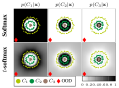
Figure 2: Toy example of a 3 class NN classifier. Color visualizes the output probability $p(C_{i}|\mathbf{x})$ on a fine grid. Top figures and bottom figures show the output of classifiers that use either softmax or $t$-softmax respectively.

Figure 1(a) visualizes this derivation for the one-dimensional binary case. Here, the softmax operator reduces to the so called sigmoid function. The graph shows how the sigmoid function tends to make mostly high confidence predictions ifnextchar,i.e.i.e.,  with $p(C_{i}|x)$ approaching either 0 or 1 for the largest part of its domain. This behaviour is certainly positive for in-distribution (IND) samples, however it persists also when $x$ is far from the means $\mu_{1}$ and $\mu_{2}$. Consequently, the sigmoid function may lead to erroneous predictions assigning high scores to OOD samples. This characteristic is also present in the multi-dimensional case and complex NN classifiers that employ the softmax operator as their output. The top scatter plots of Figure 2 show a toy example of a classifier that separates two-dimensional features into three classes. Here, the NN classifier consists of three fully connected layers with ReLU nonlinearities. This is trained using stochastic gradient descent using simulated data. As the top plots of Figure 2 show, the three classes are correctly identified. However when an OOD sample is fed to the NN, totally erroneous predictions can be given. For example in Figure 2, on the bottom left corner an OOD sample is depicted using a diamond marker. The classifier wrongly assigns this sample to the first class with a probability that equals to 1.

III The $t$-softmax operator

The bottom plots of Figure 2 show a more trustworthy classifier that does not assign high probability to OOD samples. Here, the diamond marker OOD sample is given a probability of 0.5 for the first class and 0.25 for the second and third classes. This means the uncertainty regarding this OOD sample can be directly assessed from the outputs of the classifier which can then be considered reliable confidence measures. Such a classifier is obtained by replacing the softmax operator layer with a different operator that can better model uncertainty. The key idea is to employ $t$-distributions instead of Gaussian distributions for $p(\mathbf{x}|C_{i})$:

$$p(\mathbf{x}|C_{i})=\tfrac{1}{\sqrt{\nu}B\left(\tfrac{1}{2},\tfrac{\nu}{2}\right)}\left(1+\tfrac{1}{\nu}(\mathbf{x}+\boldsymbol{\mu}_{i})^{\intercal}(\mathbf{x}+\boldsymbol{\mu}_{i})\right)^{-\tfrac{\nu+1}{2}},$$ (7)

where $B$ is the Beta function and $\nu$ is a positive real number. The choice of $t$-distribution is not arbitrary; it arises as a Gaussian distribution [22, Sec.3.2] where the variance is assumed unknown but distributed as inverse $\chi^{2}$ (parametrized by $\nu$). The $t$-distribution can be seen as a generalization of the Gaussian distributions, with (7) approaching (2) as $\nu$ increases. Indeed, the parameter $\nu$ controls how fast $t$-distribution’s tails decay. While the tails of Gaussian distribution decay exponentially those of $t$-distribution’s ones decay polynomially, hence more slowly. Such difference can be seen on the top plots of Figure 1. As a result, the $t$-distribution models uncertainty more effectively than Gaussian distributions and this can also be seen in the resulting operator named $t$-softmax, obtained substituting (7) into (1):

$$P(C_{i}|\mathbf{x})=\frac{\left(1+\tfrac{1}{\nu}\left(a+\mathbf{w}_{i}^{\intercal}\mathbf{x}+b_{i}\right)\right)^{-\tfrac{\nu+1}{2}}}{\sum_{k=1}^{N_{c}}\left(1+\tfrac{1}{\nu}\left(a+\mathbf{w}_{k}^{\intercal}\mathbf{x}+b_{k}\right)\right)^{-\tfrac{\nu+1}{2}}}.$$ (8)

In contrast to the softmax operator, in (8) $a$ does not vanish and the quadratic constraints 4, 5 and 6 are required in order to avoid complex or negative outputs. Unlike in the Gaussian case where choosing $\boldsymbol{\Sigma}=\mathbf{I}$ in 4, 5 and 6 preserves rotational invariance, here this is no longer the case. However, as the results will show this does not appear to decrease the NN classifiers accuracy. It is possible to impose 4, 5 and 6 by construction. If $\mathbf{X}\in\mathds{R}^{N\times N_{b}}$ is an input consisting of $N_{b}$ batches then the dot products inside the parenthesis of (7) and expanded as $a+\mathbf{w}_{i}^{\intercal}\mathbf{x}+b_{i}$ in (8) can be collected as:

$$\mathbf{Y}=\left(\mathbf{A}+\mathbf{W}\mathbf{X}+\mathbf{B}\right)\in\mathds{R}^{N_{c}\times N_{b}}.$$ (9)

The $(i,j)$-th elements of $\mathbf{A}$ and $\mathbf{B}$ are given by $a_{i,j}=\mathbf{x}_{j}^{\intercal}\mathbf{x}_{j}$ $b_{i,j}=1/4{\mathbf{w}}_{i}^{\intercal}{\mathbf{w}}_{i}=\boldsymbol{\mu}_{i}^{\intercal}\boldsymbol{\mu}_{i}$ for $i=1,\dots,N_{c}$ and $j=1,\dots,N_{b}$ with $\mathbf{x}_{j}$ being the $j$-th column of $\mathbf{X}$ and ${\mathbf{w}}_{i}$ being the $i$-th row of $\mathbf{W}$. Since all of the rows and columns of $\mathbf{A}$ and $\mathbf{B}$ are identical, respectively, only $N_{c}+N_{b}$ dot products are needed to construct these matrices whose full storage is not needed. Therefore, the layer defined in (9), named here as quadratic layer, does not require a substantial increase of computational resources when compared to a fully connected layer.

Figure 1(b-2) shows the resulting function for the two-dimensional binary case. Unlike the sigmoid, this function approaches 0.5 when far from $\mu_{1}$ and $\mu_{2}$ therefore promoting uncertainty on the OODs. Looking back at Figure 2 it is clear that such behaviour is reflected in the NN classifier that employs the $t$-softmax operator. Wide areas surrounding the INDs consistently give low confidence predictions. Remarkably, even though the nonlinearity of this operator is stronger with respect to the softmax operator, standard stochastic optimization methods can be employed using well known cost functions.

IV Evaluation

In this section a number of experiments is presented to support the hypothesis that $t$-softmax can lead to classifiers that are more robust to OOD samples. Additionally, it is hypothesized that $\nu=1$ should increase OOD robustness in most of the scenarios. In a more thorough formulation, $\nu$ would be related to the dimension and to the prior on the variance of the latent variables; this is a matter for future research.

IV-A Baseline and state-of-the-art

The proposed method is compared with a baseline and a state-of-the-art method. The baseline was proposed in [11] and simply consists in using the maximum of the softmax output as a confidence measure. Here, only standard fully connected layers are employed. This means that the equivalence between the softmax and the $t$-softmax operators for large $\nu$ is not reached since 5 and 6 are not satisfied. A more recent state-of-the-art method has been proposed in [14] and is known as out-of-distribution detector for neural networks (ODIN). This method consists of adding the following perturbation to the input sample $\tilde{\mathbf{x}}=\mathbf{x}-\epsilon\text{sign}\left(-\nabla_{\mathbf{x}}\log\sigma(\mathbf{x}/\gamma)\right)$ where $\sigma$ is the softmax operator, $\epsilon$ is a small constant and $\gamma$ is a scaling factor. A confidence measure is then obtained by feeding $\tilde{\mathbf{x}}$ to the classifier and taking the maximum score of the scaled softmax output. However, this technique is computationally demanding since it requires the gradient. Specifically, a forward-backward pass and an additional forward pass are needed. This means ODIN is at least three times more expensive than the baseline and the proposed method. We verified this using the NN described in Section IV-C. The average time per sample using $t$-softmax operator and ODIN is 0.44 ms and 2.58 ms respectively, meaning that with the current implementation ODIN is approximatively six times slower than the proposed method.

IV-B Evaluation metrics

Following [14] these figures of merit are used for evaluation. FPR at 95% TPR gives a measure of the possibility of OOD sample being interpreted as an IND, ifnextchar,i.e.i.e.,  the false positive rate (FPR), when the true positive rate (TPR) is 95%. Detection error (DE) is the misclassification probability when TPR is 95% and is given by $\text{DE}=0.5(1-\text{TPR})+0.5\text{FPR}$. It assumes IND and OOD samples are equal in number. AUROC is the Area Under the Receiver Operating Characteristic curve (AUROC). The ROC curve [23] is the plot between TPR and FPR at different operating points of the classifier. Larger area under this curve implies more robust classifiers. AUPR is the Area Under the Precision-Recall curve (AUPR). Similarly, the PR curve [24] is the plot between precision ($\text{TP}/(\text{TP+FP})$) and recall ($\text{TP}/(\text{TP}+\text{FN})$) at different operating points.

IV-C Result on FMNIST and KMNIST

The proposed method is evaluated on two image classification tasks using Fashion-MNIST (FMNIST) [25] and Kuzushiji-MNIST (KMNIST) [26] datasets. These are datasets of images of clothes and cursive Japanese Hiragana characters respectively and are both intended as a more challenging replacement of the well-known MNIST dataset [27]. For these experiments a standard convolutional neural network (CNN) [28] is used. Its architecture consists of two two-dimensional convolutional layers with 20 and 50 channels respectively having two-dimensional max pooling and ReLU nonlinearities. The convolutional layers are followed by three fully connected layers that successively reduce the latent variable dimensions from $800$ to $500$, $100$ and $10$. ReLU nonlinearities are also employed between these layers. When $t$-softmax is used the last fully connected layer is replaced by the quadratic layer described in Section III. Classifiers are trained using PyTorch [29] in a reproducible manner [30]. Specifically, stochastic gradient descent is used with Nesterov acceleration, weight decay of $5\cdot 10^{-4}$, momentum of $0.5$, batches of 128 samples, a learning rate of $0.1$ for $20$ epochs using cross entropy as loss function.

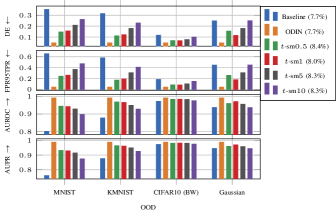
Figure 3: Results for a FMNIST classifier. Arrows on the y-axis labels indicate if the figure of merit should be either positive or negative for the classifier to be more robust. In the legend, $t$-sm stands for $t$-softmax and the number next to the abbreviation is value of $\nu$. Percentages between parenthesis in the legend indicate the test error.

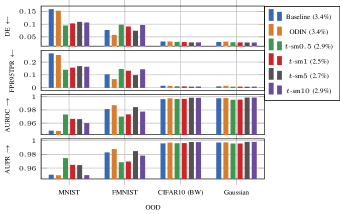
Figure 4: Results for a KMNIST classifier.

Figure 3 shows plots of the different figures of merit for the FMNIST classifier. The classifiers that utilize $t$-softmax have been trained using different values of $\nu$ to check the effect of this parameter. Looking at the percentages in the legend that indicate the test error of the classifiers, similar performances are reached with slightly worse test errors for the classifiers with $t$-softmax. The confidence measures are obtained from the IND test dataset and different OOD datasets such as MNIST, KMNIST, gray scale CIFAR10 [31] and Gaussian noise. An equal number of IND and OOD samples is used. These confidence measures are then used to evaluate the robustness of the classifiers using the figures of merit described in Section IV-B. The performance of ODIN is superior, however $t$-softmax sometimes evens ODIN for example when CIFAR10 is used as OOD. Similar results can be seen in Figure 4 that shows the same figures of merit for the KMNIST classifiers. Here FMNIST is also used as an OOD dataset. It can be seen that in this case slightly better test error are achieved by the $t$-softmax classifiers. However, the baseline is not surpassed by all $t$-softmax classifier configurations. Specifically, when FMNIST is the OOD dataset $t$-softmax has inferior figures of merit with respect to the baseline, but not in the case $\nu=5$ where it reaches slightly better results. Overall, ODIN reaches results that are very close to the ones of the $t$-softmax classifiers. ODIN is superior only when FMNIST is the OOD dataset but is inferior with MNIST. In conclusion, it can be seen that all $t$-softmax classifiers consistently outperform the baseline, with $\nu=1$ giving the overall best performances, confirming the hypothesis that this setting can be used in practice.

IV-D Result on CIFAR10

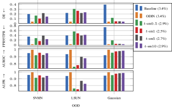
Figure 5: Results for a CIFAR10 classifier using Densenet.

A more advanced state-of-the-art NN known as Densenet [32] with a depth of 100 is trained on CIFAR10 [31], a dataset consisting of coloured $32\times 32$ pixel images of objects belonging to 10 different classes. A similar training procedure as the one described in Section IV-C is used, with 300 epochs, batch size of 64 and a weight decay of $10^{-5}$. Learning rate is decreased by a factor of 10 at the $150$th and $225$th epoch. Here different OOD datasets are used: SVHN [33] and resized images of the LSUN test set [34]. Figure 5 shows the evaluation results. The results are less convincing when compared to the previous experiments. In particular, when the OOD dataset is the LSUN dataset $t$-softmax reaches performance that are below the baseline. However, the same conclusions of Section IV-C are supported by the Gaussian OOD experiment where significant improvements are seen.

V Conclusion

In this paper a novel operator named $t$-softmax is proposed. It is shown that its statistical derivation is analogous to the one used for the softmax operator with the only difference that $t$-distribution are used to better model uncertainty. Results on image classification tasks show that classifiers trained using $t$-softmax can be robust to OOD samples. The proposed method is sometimes comparable to a state-of-the-art method named ODIN which is at least three times more computationally expensive. It is envisaged that in the cases where $t$-softmax fails to outperform the baseline, further modifications of the NN architectures and better understanding of the effect of the parameter $\nu$ could lead to more positive results.

References

- [1] J. Han, D. Zhang, G. Cheng, N. Liu, and D. Xu, “Advanced deep-learning techniques for salient and category-specific object detection: a survey,” IEEE Signal Process. Magazine, vol. 35, no. 1, pp. 84–100, 2018.
- [2] A. Mesaros, T. Heittola, E. Benetos, P. Foster, M. Lagrange, T. Virtanen, and M. D. Plumbley, “Detection and classification of acoustic scenes and events: Outcome of the dcase 2016 challenge,” IEEE/ACM Trans. Audio, Speech Lang. Process., vol. 26, no. 2, pp. 379–393, 2017.
- [3] H. Purwins, B. Li, T. Virtanen, J. Schlüter, S. Y. Chang, and T. Sainath, “Deep learning for audio signal processing,” IEEE J. Selected Topics in Signal Process., vol. 13, no. 2, pp. 206–219, 2019.
- [4] M. J. Bianco, P. Gerstoft, J. Traer, E. Ozanich, M. A. Roch, S. Gannot, and C.-A. Deledalle, “Machine learning in acoustics: Theory and applications,” J. Acoustical Soc. America, vol. 146, no. 5, pp. 3590–3628, 2019.
- [5] G. Hinton, L. Deng, D. Yu, G. E. Dahl, A. R. Mohamed, N. Jaitly, A. Senior, V. Vanhoucke, P. Nguyen, T. N. Sainath et al., “Deep neural networks for acoustic modeling in speech recognition: The shared views of four research groups,” IEEE Signal Process. Magazine, vol. 29, no. 6, pp. 82–97, 2012.
- [6] W. Xiong, J. Droppo, X. Huang, F. Seide, M. L. Seltzer, A. Stolcke, D. Yu, and G. Zweig, “Toward human parity in conversational speech recognition,” IEEE/ACM Trans. Audio, Speech Lang. Process., vol. 25, no. 12, pp. 2410–2423, 2017.
- [7] A. Nguyen, J. Yosinski, and J. Clune, “Deep neural networks are easily fooled: High confidence predictions for unrecognizable images,” in Proc. Conf. Computer Vision Pattern Recognition (CVPR), 2015.
- [8] D. Hendrycks, M. Mazeika, and T. G. Dietterich, “Deep anomaly detection with outlier exposure,” in Proc. Int. Conf. Learning Representations (ICLR), 2019.
- [9] K. Lee, H. Lee, K. Lee, and J. Shin, “Training confidence-calibrated classifiers for detecting out-of-distribution samples,” in Proc. Int. Conf. Learning Representations (ICLR), 2018.
- [10] M. Hein, M. Andriushchenko, and J. Bitterwolf, “Why ReLU networks yield high-confidence predictions far away from the training data and how to mitigate the problem,” in Proc. Conf. Computer Vision Pattern Recognition (CVPR), 2019.
- [11] D. Hendrycks and K. Gimpel, “A Baseline for Detecting Misclassified and Out-of-Distribution Examples in Neural Networks,” in Proc. Int. Conf. Learning Representations (ICLR), 2017.
- [12] Y. Gal and Z. Ghahramani, “Dropout as a Bayesian Approximation: Representing Model Uncertainty in Deep Learning,” in Proc. Int. Conf. Machine Learning (ICML), 2016.
- [13] A. Vyas, N. Jammalamadaka, X. Zhu, D. Das, B. Kaul, and T. L. Willke, “Out-of-distribution detection using an ensemble of self supervised leave-out classifiers,” in Proc. European Conf. Computer Vision (ECCV), 2018.
- [14] S. Liang, Y. Li, and R. Srikant, “Enhancing the reliability of out-of-distribution image detection in neural networks,” in Proc. Int. Conf. Learning Representations (ICLR), 2018.
- [15] A. Kendall and Y. Gal, “What uncertainties do we need in Bayesian deep learning for computer vision?” in Conf. Neural Inf. Process. Syst. (NIPS), 2017.
- [16] T. DeVries and G. W. Taylor, “Learning confidence for out-of-distribution detection in neural networks,” arXiv preprint arXiv:1802.04865, 2018.
- [17] M. D. Bedworth and A. J. Heading, “The importance of models in Bayesian data fusion,” in Proc. IEEE Conf. Control Applications, 1992, pp. 13–16.
- [18] W. Liu, Y. Wen, Z. Yu, M. Li, B. Raj, and L. Song, “Sphereface: Deep hypersphere embedding for face recognition,” in Proc. Conf. Computer Vision Pattern Recognition (CVPR), 2017.
- [19] F. Wang, J. Cheng, W. Liu, and H. Liu, “Additive margin softmax for face verification,” IEEE Signal Process. Letters, vol. 25, no. 7, pp. 926–930, 2018.
- [20] K. Asadi and M. L. Littman, “An alternative softmax operator for reinforcement learning,” in Proc. Int. Conf. Machine Learning (ICML), 2017.
- [21] J. S. Bridle, “Probabilistic interpretation of feedforward classification network outputs, with relationships to statistical pattern recognition,” in Neurocomputing. Springer, 1990, pp. 227–236.
- [22] A. Gelman, J. B. Carlin, H. S. Stern, D. B. Dunson, A. Vehtari, and D. B. Rubin, Bayesian data analysis, 3rd ed. CRC Press, 2014.
- [23] T. Fawcett, “An introduction to ROC analysis,” Pattern Recognition Letters, vol. 27, no. 8, pp. 861–874, 2006.
- [24] T. Saito and M. Rehmsmeier, “The precision-recall plot is more informative than the ROC plot when evaluating binary classifiers on imbalanced datasets,” PloS one, vol. 10, no. 3, 2015.
- [25] H. Xiao, K. Rasul, and R. Vollgraf, “Fashion-MNIST: a Novel Image Dataset for Benchmarking Machine Learning Algorithms,” arXiv preprint arXiv:1708.07747, 2017.
- [26] T. Clanuwat, M. Bober-Irizar, A. Kitamoto, A. Lamb, K. Yamamoto, and D. Ha, “Deep learning for classical japanese literature,” arXiv preprint arXiv:1812.01718, 2018.
- [27] Y. LeCun, L. Bottou, Y. Bengio, and P. Haffner, “Gradient-based learning applied to document recognition,” in Proc. of the IEEE, vol. 86, no. 11, 1998, pp. 2278–2324.
- [28] Y. LeCun, B. Boser, J. S. Denker, D. Henderson, R. E. Howard, W. Hubbard, and L. D. Jackel, “Backpropagation applied to handwritten zip code recognition,” Neural computation, vol. 1, no. 4, pp. 541–551, 1989.
- [29] A. Paszke, S. Gross, S. Chintala, G. Chanan, E. Yang, Z. DeVito, Z. Lin, A. Desmaison, L. Antiga, and A. Lerer, “Automatic differentiation in PyTorch,” in Proc. Conf. Neural Inf. Process. Syst. (NIPS), 2017.
- [30] N. Antonello. (2020) Implementation of -softmax operator using PyTorch. [Online]. Available: https://github.com/idiap/tsoftmax
- [31] A. Krizhevsky, “Learning multiple layers of features from tiny images,” Technical report, University of Toronto, 2009.
- [32] G. Huang, Z. Liu, L. Van Der Maaten, and K. Q. Weinberger, “Densely connected convolutional networks,” in Proc. Conf. Computer Vision Pattern Recognition (CVPR), 2017.
- [33] Y. Netzer, T. Wang, A. Coates, A. Bissacco, B. Wu, and A. Y. Ng, “Reading digits in natural images with unsupervised feature learning,” in Proc. Conf. Neural Inf. Process. Syst. (NIPS), 2011.
- [34] F. Yu, A. Seff, Y. Zhang, S. Song, T. Funkhouser, and J. Xiao, “LSUN: Construction of a large-scale image dataset using deep learning with humans in the loop,” arXiv preprint arXiv:1506.03365, 2015.