Jordan Jalving
jalving@wisc.edu
Sungho Shin
sungho.shin@wisc.edu
Victor M. Zavala
victor.zavala@wisc.edu
22institutetext: Department of Chemical and Biological Engineering
University of Wisconsin-Madison, 1415 Engineering Dr, Madison, WI 53706, USA
A Graph-Based Modeling Abstraction for Optimization:
Concepts and Implementation in Plasmo.jl
Abstract
We present a general graph-based modeling abstraction for optimization that we call an OptiGraph. Under this abstraction, any optimization problem is treated as a hierarchical hypergraph in which nodes represent optimization subproblems and edges represent connectivity between such subproblems. The abstraction enables the modular construction of highly complex models in an intuitive manner, facilitates the use of graph analysis tools (to perform partitioning, aggregation, and visualization tasks), and facilitates communication of structures to decomposition algorithms. We provide an open-source implementation of the abstraction in the Julia-based package Plasmo.jl. We provide tutorial examples and large application case studies to illustrate the capabilities.
Keywords: graph theory, optimization, modeling, structure, decomposition
1 Motivation and Background
Advances in decomposition algorithms and computing architectures are continuously expanding the complexity and scale of optimization models that can be tackled Kang2014 . Application examples include financial planning Gondzio2006 , supply chain scheduling Maravelias2012 , enterprise-wide management Grossmann2012 , infrastructure optimization kang2015 , and network control rawlings2009 . Decomposition algorithms seek to address computational bottlenecks (in terms of memory, robustness, and speed) by exploiting structures present in a model Scattolini2009 ; Zavala2016 ; Brunaud2017 ; Conejo2006 ; Cao2019 . Well-known algorithms to exploit structures at the problem level include Lagrangian decomposition Fisher1985 , Benders decomposition Sahinidis1991 , Dantzig-Wolfe decomposition Bergner2015 , progressive hedging Watson2012 , Gauss-Seidel shin2018multi , and the alternating direction method of multipliers Boyd2011 . Fundamentally, these algorithms seek to solve the original problem by solving subproblems defined over subproblem partitions and by coordinating subproblem solutions via communication of primal-dual information. Well-known paradigms to exploit structures at the linear-algebra level (inside optimization solvers) include block elimination and preconditioning (e.g., Schur and Riccati) Gondzio2003 ; Kang2014 ; Rodriguez2020 ; rao1998application . In these schemes, the original problem is solved by using a general algorithm (e.g., interior-point, sequential quadratic programming, or augmented Lagrangian) and decomposition occurs during the computation of the search step.
The efficient use of decomposition algorithms (and of computing architectures under which they are executed) relies on the ability to communicate model structures in a flexible manner. Surprisingly, the development of modeling environments that support the development of decomposition algorithms has remained rather limited. As a result, decomposition algorithms have been mostly used to tackle models that have rather obvious structures such as stochastic optimization Linderoth2003 ; Kim2016 ; Steinbach2003 ; Lubin2012 ; Hubner2020 , network optimization Shin2019 , dynamic optimization biel2019efficient , and hierarchical optimization grossman2013 . Some examples of environments that support structured modeling include the structure-conveying modeling language (SML) Colombo2009 , which is an extension of AMPL ampl that conveys structures in the form of variable and constraint blocks. SML was one of the earliest attempts to automate structure identification and exploitation in modeling environments and was motivated by the availability of structure-exploiting interior point solvers. Pyomo hart2017pyomo is a Python-based modeling package that enables the expression of structures in the form of variable and constraint blocks. Pyomo also provides a structured modeling template called PySP Watson2012 that greatly facilitates the expression of multi-stage stochastic programs and their solution using progressive hedging and Benders decomposition. StuctJuMP Huchette2014 and StochasticPrograms.jl biel2019efficient are extensions of the Julia-based package JuMP.jl DunningHuchetteLubin2017 to express stochastic optimization structures.
1.1 Graph-Based Model Representations
It is important to recall that, at a fundamental level, an optimization model is a collection of algebraic functions (constraints and objectives) that are connected via variables. Connectivity between functions and variables can be represented as graphs. This concept is by no means new; graph representations of optimization models are routinely used in modeling environments to perform automatic differentiation and model processing tasks ampl . The underlying graph structure of the model is also implicitly communicated to solvers in the form of sparsity patterns of constraint, objective, and derivative matrices. However, these graph representations operate at a level of granularity that might not be particularly useful for decomposition. Specifically, the benefits of decomposition tend to become apparent when operating over blocks of functions and variables. An issue that arises here is that identifying blocks that are suitable for a decomposition algorithm and computing architecture is not an easy task. For instance, we might want to identify blocks that have sparse external connectivity (to reduce the amount of inter-block coupling) Rodriguez2020 . Moreover, if decomposition is to be executed on a parallel computer, one might want to ensure that the blocks are of similar size (to avoid load imbalance issues) kim2019asynchronous . Another issue that arises here is that blocks might be degenerate (e.g., they might have more constraints than variables). Existing modeling environments do not provide capabilities to handle such issues.
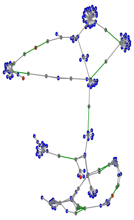
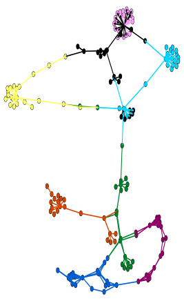
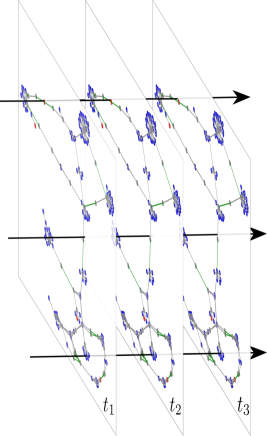
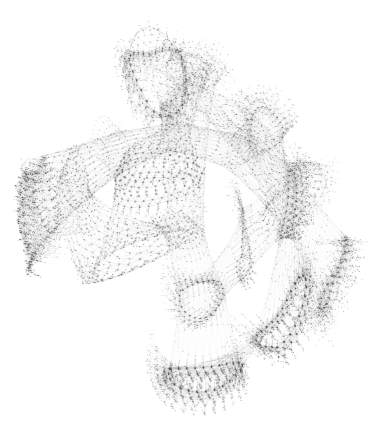
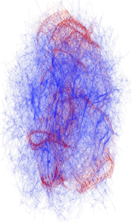
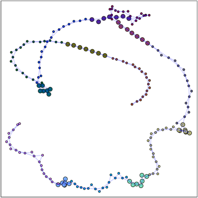
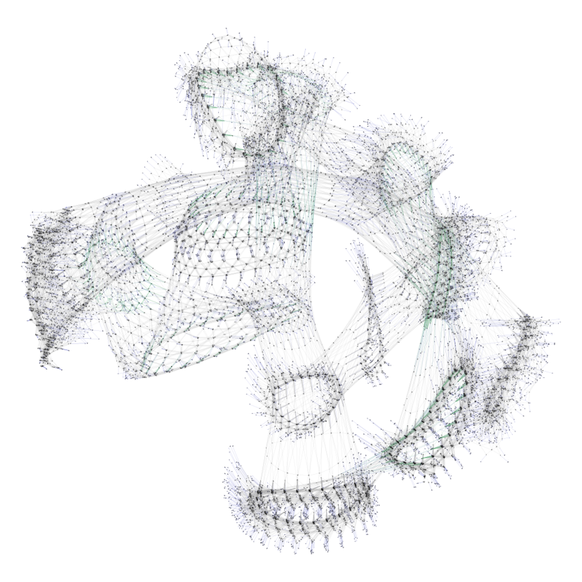
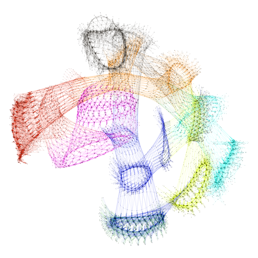
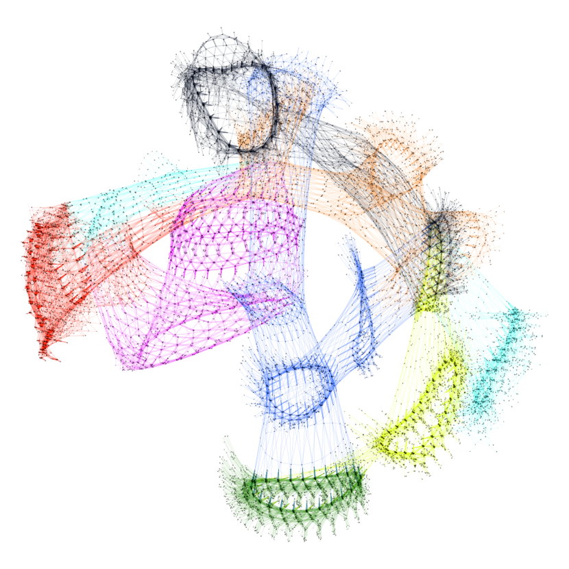
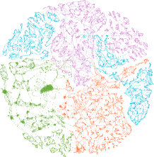
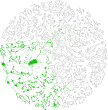
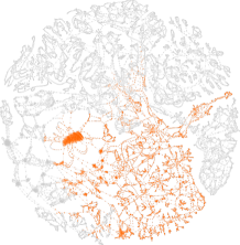
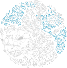
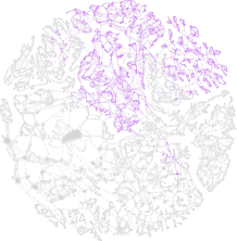
To highlight some of the challenges that arise in the modeling structured problems, consider the natural gas network depicted in the left panel of Figure 1(a). This is a regional gas transmission system that contains 215 pipelines, 16 compressors, 172 junction points Chiang2016 . The problem has an obvious structure induced by the network topology. This representation naturally conveys connectivity between components (pipelines, compressors, and junctions). Hidden in this representation, however, is the internal connectivity present in such components; this inner connectivity is usually complex and induced by variables and constraints that capture physical coupling (e.g., conservation of mass, energy, and momentum). The issue here is that there is a severe imbalance in the complexity of the components (e.g, pipelines might contain partial differential equations to capture flow while compressors contain much simpler algebraic equations). Moreover, hidden in the representation is the connectivity of the components across time, which gives rise to complex space-time coupling. Intuitively, one could seek to decompose the model spatially by exploiting the network topology, as shown in the middle panel of Figure 1(b). Unfortunately, this approach does not account for inner component complexity and results in partitions with a disparate number of variables and constraints. This will give rise to load balancing issues and limit the benefits of parallel computation. To deal with this issue, one could seek to decompose the problem temporally, as shown in the right panel of Figure 1(c). This approach leads to well-balanced partitions (every partition is a copy of the network), but leads to significantly more coupling between partitions. A high degree of coupling will also limit the scalability of algorithms (increased coupling tends to increase communication and slow down convergence). One would intuitively expect that there exist partitions that can balance coupling and load balancing (by traversing space-time and exploiting inner block complexity). Identifying such partitions, however, requires unfolding of the model structure. Figure 2(a) provides a visual rendering of the spatial representation of the natural gas system that unfolds inner component connectivity. Here, the size of the clusters gives us an initial indication of component complexity. Figure 2(b) is a visual rendering of the space-time representation that further unfolds temporal connectivity between components and this clearly reveals interesting (but complex) structures. Determining effective partitions from such structures requires advanced graph partitioning techniques.
So the question is: If an optimization model is a graph after all, why is it that we do not use graph concepts to build optimization models? Most optimization modelers follow an algebraic modeling paradigm in which the model is assembled by adding functions and variables (e.g., using packages such as GAMS, AMPL, Pyomo). There is, however, another modeling paradigm known as object-oriented modeling, in which the model is assembled by adding blocks of functions and variables. This paradigm is widely used in engineering communities to perform simulation (e.g., using packages such as Modelica, AspenPlus, and gProms mattsson1998physical ; dowling2015framework ). An important observation is that object-oriented modeling more naturally lends itself to the expression and exploitation of problem structures because the underlying graph is progressively built by the user. For instance, packages such as AspenPlus use the underlying graph structure induced by blocks to partition the model and communicate it to a decomposition algorithm. One could thus think of object-oriented modeling as a form of graph-based modeling. The purely object-oriented paradigm however, may suffer from imblance of component complexity or from a high degree of coupling when performing decomposition.
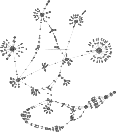
Recently, we proposed a graph-based abstraction to build optimization models Jalving2017 ; Jalving2019 . In this abstraction, any optimization model is treated as a hierarchical graph. At a given level, a graph comprises a set of nodes and edges; each node contains an optimization model (with variables, objectives, constraints, and data) and each edge captures connectivity between node models. Importantly, the optimization model in each node can be expressed algebraically (as in a standard algebraic modeling language) or as a graph (thus enabling inheritance and creation of hierarchical graphs). This provides flexibility to capture both algebraic and object-oriented modeling paradigms under the same framework. The abstraction naturally exposes problem structure to algorithms and provides a modular approach to construct models. Modularization enables collaborative model building, independent processing of model components (e.g., automatic differentiation), and data management. The abstraction naturally captures a wide range of problem classes such as stochastic optimization (graph is a tree), dynamic optimization (graph is a line), network (graph is the network itself), PDE optimization (graph is a mesh), and multiscale optimization (graph is a meshed tree). Moreover, graphs can be naturally built by combining graphs from different classes (e.g., stochastic PDE optimization). This approach is thus more general than other graph-based abstractions proposed for specific problem classes such as network optimization and control Heo2014 ; Jogwar2015 ; Moharir2017 ; Tang2018 ; Hallac2015 . This modeling abstraction also generalizes those used in simulation packages such as Modelica, AspenPlus, gProms, which are tailored to specific physical systems. The hierarchical graph structure can be communicated to decomposition solvers or it can be collapsed into an optimization model that can be solved with off-the-shelf solvers (e.g., Gurobi or Ipopt). To illustrate the types of capabilities enabled by hierarchical graph modeling, we take the natural-gas network in Figure 1(a) and couple it to an electrical network, as shown in Figure 3(a). Here, the natural gas graph and the electrical power graph can be built independently and then coupled to construct a higher level graph. The graph structure can be communicated to a graph visualization tool and this allows us to analyze the graph using different representations. In the left panel we see a traditional representation of infrastructure coupling (that hides temporal and component coupling), while in the middle and right panels we unfold spatial and spatio-temporal coupling. The space-time graph contains over 100,000 nodes and 300,000 edges and reveals that there exist a large number of non-obvious structures that might be beneficial from a computational standpoint.
Graph-based model representations can take advantage of powerful graph analysis tools. For instance, graph partitioning tools such as Metis Karypis1998 and Scotch pellegrini provide efficient algorithms to automatically analyze problem structure and to identify suitable partitions to be exploited by decomposition algorithms. Graph partitioning seeks to decompose a domain described by a graph such that communication between subdomains is minimized subject to load balancing (i.e., the domains are about the same size). The most ubiquitous graph partitioning applications target parallelizing scientific simulations schloegel2003 , performing sparse-matrix operations Gupta1997 , and preconditioning systems of PDEs Schulz15coursenotes . Hypergraph partitioning generalizes graph partitioning concepts to effectively decompose non-symmetric domains Devine2006 and has been applied to physical network design and sparse-matrix-vector multiplication Papa2007 . Popular hypergraph partitioning tools include hMetis KarypishMetis and PaToH Çatalyürek2011 . Community detection approaches have also been used to find partitions that maximize modularity Newman2006 ; Allman2018 . Graph partitioning approaches have been used to decompose optimization problems in various contexts. Graph approaches have been used to partition network optimization problems using graph coloring techniques Zenios1988 and block partitioning schemes Zenios1992 . Bipartite graph representations have been used to permute linear programs Ferris1998 into block diagonal form to enable parallel solution. Hypergraph partitioning has been used to decompose mixed-integer programs to formulate Dantzig-Wolfe decompositions Wang2013 ; Bergner2015 using hMetis and PaToH. Community detection approaches have been used to automate structure identification in general optimization problems and with this enable higher efficiency of decomposition algorithms Tang2017 ; Allman2018 . We highlight that these approaches start with a given algebraic optimization model that is then transformed into a graph representation; consequently, these are not graph modeling abstractions per se.
Graph-based representations have been adopted in modeling environments for specific problem classes. SnapVX Hallac2015 uses a graph topology abstraction to formulate network optimization problems that are solved using ADMM Boyd2011 . GRAVITY Hijazi2018 is an algebraic modeling framework that incorporates graph-aware modeling syntax but this is not the paradigm driving the environment. DISROPT is a Python-based environment for distributed network optimization Farina . DeCODe decode is a package written in Matlab and Python that automatically creates a bipartite representation of optimization models created with Pyomo and uses community detection to determine partitions for use with Benders or Lagrangian decomposition. In recent work we have provided a Julia-based implementation of our hierarchical graph abstraction, that we called Plasmo.jl Jalving2017 ; Jalving2019 . This package provides modeling syntax to systematically create hierarchical graph models, to integrate algebraic JuMP.jl DunningHuchetteLubin2017 models within nodes, and to facilitate the expression of connectivity between node models. The first version of Plasmo.jl used an abstraction that was targeted to handle coupled infrastructure networks. This abstraction sought to generalize the network modeling capabilities of DMNetwork abhyankar2018petsc (used for simulation) to handle optimization problems Jalving2017 . Subsequent development provided data management capabilities to facilitate model reduction and re-use (for real-time optimization applications) Jalving2018 and provided an interface to communicate graph structures to the parallel interior-point solver PIPS-NLP cao2017scalable . The abstraction was later used to create a computational graph abstraction wherein nodes are computational tasks and edges communicate data between tasks. This abstraction enables hierarchical modeling of cyber-physical systems, workflows, and algorithms Jalving2019 .
1.2 Contributions of This Work
In this work, we present a new and general graph modeling abstraction for optimization that we call an OptiGraph. As in our previously proposed abstraction, we represent any optimization model as a hierarchical graph wherein nodes contain optimization models with corresponding objectives, variables, constraints, and data. The novel feature of our abstraction lies on how edge connectivity between models is represented. Specifically, we express connectivity in the form of hyperedges (edges that can connect multiple nodes), thus generalizing the concept of an edge (which connects two edges). This hypergraph representation enables a more intuitive expression of structures at the modeling level and enables the use of efficient hypergraph analysis tools. The hypergraph representation can also be transformed into a standard graph representation (via lifting) and to other graph representations (e.g., bipartite) and this enables the use of different graph analysis techniques and tools and enables flexible expression of structures for decomposition. We provide an efficient implementation of the OptiGraph abstraction in Plasmo.jl that can handle hundreds of thousands to millions of nodes and edges. We implement an interface to LightGraphs.jl and Gephi to demonstrate that the implementation facilitates interfacing to graph analysis and visualization tools Bromberger17 ; gephi . We illustrate how to use these tools and topological information obtained from the OptiGraph to automatically obtain partitions that trade-off coupling and load balancing and to compute useful descriptors of the graph (e.g., neighborhoods, degree distribution, minimum spanning tree, modularity). Moreover, we show how to manipulate the graph to perform aggregation functions (merge nodes). These features provide flexibility to visualize, decompose, and solve large models using different techniques. We implement an interface to the parallel solver PIPS-NLP to analyze computational efficiency obtained with different partitioning strategies. We also demonstrate that the abstraction facilitates the implementation of decomposition algorithms; to do so, we implement an overlapping Schwarz scheme that is tailored to graph-structured problems Shin2020 .
1.3 Paper Structure
The rest of the paper is organized as follows: Section 2 describes the OptiGraph abstraction and its implementation in Plasmo.jl. In Section 3 we show how the OptiGraph structure can be exploited by different optimization algorithms. Section 4 provides case studies that demonstrate capabilities on a large natural gas network problem and on a direct current optimal power flow (DC OPF) problem. Section 5 concludes the manuscript and discusses future directions for Plasmo.jl.
2 Hierarchical Graph Abstraction and Implementation
This section introduces the OptiGraph abstraction alongside its implementation in Plasmo.jl. In a nutshell, Plasmo.jl is a graph-structured modeling language that offers concise syntax and access to graph tools that enable model analysis and manipulation (e.g., partitioning, aggregation, visualization). Plasmo.jl is an official Julia package hosted at https://github.com/zavalab/Plasmo.jl. All example scripts in this section can be found at https://github.com/zavalab/JuliaBox/tree/master/PlasmoExamples.
2.1 Graph Abstraction
The OptiGraph abstraction proposed is composed of a set of OptiNodes (each embedding an optimization model with its local variables, constraints, objective function, and data) and a set of OptiEdges (each embedding a set of linking constraints) that capture coupling between OptiNodes. The OptiGraph is denoted as and contains the optimization model of interest. The OptiEdges are hyperedges that connect two or more OptiNodes. The OptiGraph is an undirected hypergraph. Whenever clear from context, we simply refer to the OptiGraph as graph, to the OptiNodes as nodes, and to OptiEdges as edges. We denote the set of nodes that belong to as and the set of edges as . The topology of the hypergraph is encoded in the incidence matrix ; here, the notation denotes cardinality of set . The neighborhood of node is denoted as and this is the set of nodes connected to . The set of nodes that support an edge are denoted as and the set of edges that are incident to node are denoted as .
The optimization model associated with an OptiGraph can be represented mathematically as:
| (2.1a) | |||||
| s.t. | (2.1b) | ||||
| (2.1c) | |||||
Here, is the collection of decision variables over the entire set of nodes and is the set of variables on node . Function (2.1a) is the graph objective function which is given by the sum of objective functions , (2.1b) represents the collection of constraints over all nodes , and (2.1c) is the collection of linking constraints over all edges . Here, the constraints of a node are represented by the set while the linking constraints induced by an edge are represented by the vector function (an edge can contain multiple linking constrains). The optimization problem representation captures sufficient features to facilitate the discussion but differs from the actual implementation. For example, here we assume that the graph objective is obtained via a linear combination of the node objectives but other combinations are possible (e.g., to handle conflict resolution formulations wherein nodes represent different stakeholders). In addition, we assume that coupling between nodes arises in the form of complicating constraints but definition of complicating variables is also possible (coupling variables can always be represented as coupling constraints via lifting).
2.2 Syntax and Usage
We now introduce the Plasmo.jl implementation of the OptiGraph and show how to use its syntax to create, analyze, and solve an optimization model. Plasmo.jl implements the graph model described by (2.1) and illustrated in Figure 4. In our implementation, an OptiNode encapsulates a Model object from the JuMP.jl modeling language. This harnesses the algebraic modeling syntax and processing functionality of JuMP.jl. An OptiEdge object encapsulates the linking constraints that define coupling between the nodes.
.
2.2.1 Example 1 : Creating an OptiGraph
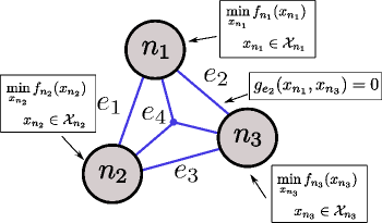
We start with the simple example given by (2.2) to demonstrate OptiGraph syntax:
| (Objective) | (2.2a) | ||||
| s.t. | (Node 1 Constraints) | (2.2b) | |||
| (Node 2 Constraints) | (2.2c) | ||||
| (Node 3 Constraints) | (2.2d) | ||||
| (Link Constraint) | (2.2e) | ||||
In this model, equations (2.2b), (2.2c), and (2.2d) represent individual node constraints and (2.2e) is a linking constraint that couples the three nodes. We formulate and solve this optimization model as shown in Snippet 1. We import Plasmo.jl into a Julia session on Line 1 as well as the off-the-shelf linear programming solver GLPK glpk to solve the problem. We define graph1 (an OptiGraph) on Line 5 and then create three OptiNodes on Lines 8-24 using the @optinode macro. We also use the @variable, @constraint, and @objective macros (extended from JuMP.jl) to define node model attributes. Next, we use the @linkconstraint macro on Line 27 to create a linking constraint between the three nodes. Importantly, this automatically creates an OptiEdge. This feature is key, as the user does not need to express the topology of the graph (this is automatically created behind the scenes as linking constraints are added). In other words, the user does not need to provide an adjacency matrix (which can be highly complex). We solve the problem using the GLPK optimizer on Line 30. Since GLPK does not exploit graph structure, Plasmo.jl automatically transforms the graph into a standard LP format. We query the solution for each variable using the value function on Line 33 which accepts the corresponding node and variable we wish to query. Another important feature is that the solution data retains the structure of the OptiGraph, and this facilitates query and analysis. We also highlight that the syntax is similar to that of JuMP.jl but operates at a higher level of abstraction.
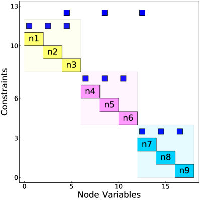
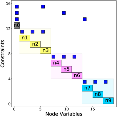
We have implemented capabilities to visualize the structure of OptiGraphs by extending plotting functions available in Plots.jl. We layout the OptiGraph topology on Line 39 using the plot function and we plot the underlying adjacency matrix structure on Line 44 using the spy function. Both of these functions can accept keyword arguments to customize their layout or appearance. The matrix visualization also encodes information on the number of variables and constraints in each node and edge. The results are depicted in Figure 5; the left figure shows a standard graph visualization where we draw an edge between each pair of nodes if they share an edge, and the right figure shows the matrix representation where labeled blocks correspond to nodes and blue marks represent linking constraints that connect their variables. The node layout helps visualize the overall connectivity of the graph while the matrix layout helps visualize the size of nodes and edges.
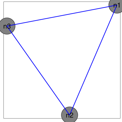
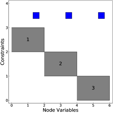
function (left) and graph matrix representation obtained with spy function (right).
2.3 Hierarchical Graphs
A key novelty of the OptiGraph abstraction is that it can cleanly represent hierarchical structures. This feature enables expression of models with multiple embedded structures and
enables modular model building (e.g., by merging existing models).
To illustrate this, consider you have the Optigraphs each with its own local nodes and edges. We assemble these low-level OptiGraphs (subgraphs) to
build a high-level OptiGraph
. We use the notation to indicate that the high-level
graph has nodes and edges
. Here,
are global edges in (connect nodes across low-level graphs but are not elements of such subgraphs) and are global
nodes in (can be connected to nodes in low-level graphs but that are not elements of such subgraphs).
For every global edge , we have that , , and where
.
In other words, the edges only connect nodes across low-level graphs and or between global
nodes in and low-level graphs. Consequently, if we treat the elements of a node set as a graph (i.e., we combine subgraphs into a single OptiNode),
we can represent as . This nesting procedure can be carried over multiple levels to form a hierarchical graph.
The formulation given by (2.1) can be extended to describe a hierarchical graph with an arbitrary number of subgraphs. This is shown in (2.3); here, represents the collection of variables over the entire set of nodes in the graph. Equation (2.3c) are the linking constraints over the edges for each subgraph. Here, we use the notation to indicate that the subgraph elements are part of the recursive set of subgraphs in (i.e., set contains all subgraphs in the graph). Specifically, we define the mapping } where is the total number of subgraphs in .
| (2.3a) | |||||
| s.t. | (2.3b) | ||||
| (2.3c) | |||||
| (2.3d) | |||||
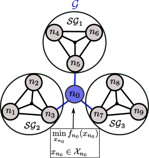
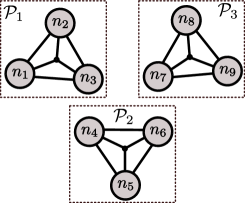
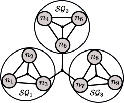
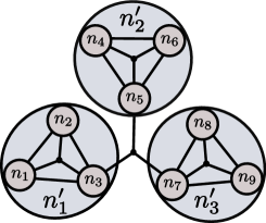
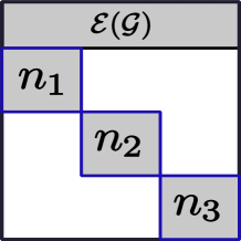
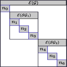
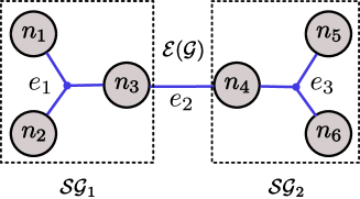
Figures 6 and 7 depict examples of graphs with subgraph nodes. In Figure 6 we have a graph that contains three subgraphs with a total of nine nodes (three in each subgraph). The graph contains a global hyperedge that connects to local nodes in the subgraphs. Figure 7 shows a hierarchical graph with three subgraphs and nine total nodes. The graph contains a global node that is connected to nodes in the subgraphs. This type of structure arises when there is a parent (master) optimization problem that is connected to children subproblems.
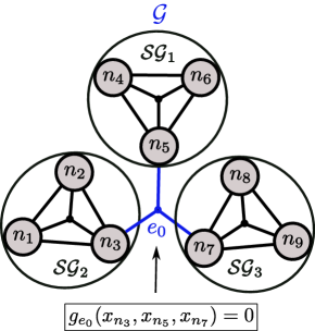
2.3.1 Example 2: Hierarchical Graph with Global Edge
An OptiGraph object manages its own nodes and edge in a self-contained manner (without requiring references to other higher-level graphs). Consequently, we can define subgraphs independently (in a modular manner) and these can be coupled together by using global edges or nodes defined on a high-level graph. This feature is key because each node can have its own syntax (syntax does not need to be consistent or non-redundant over the entire model). This is a fundamental difference with algebraic modeling languages (syntax has to be consistent and non-redundant over the entire model). The formulation in (2.4) illustrates how to express hierarchical connectivity using a global edge. Equation (2.4a) is the summation of every node objective function in the graph; (2.4b), (2.4c) and (2.4d) describe node constraints; (2.4e), (2.4f), and (2.4g) represent link constraints within each subgraph; and (2.4h) defines a link constraint at the higher level graph (that links nodes from each individual subgraph). Formulation (2.4) can be expressed as a hierarchical OptiGraph using the add_subgraph! function. This functionality is shown in Code Snippet 2, where we extend graph1 from Code Snippet 1. We create a new graph called graph2 on Line 2 and setup nodes and link them together on Lines 4 through 17. We also construct graph3 in the same fashion on Lines 20 through 35. Next, we create graph0 on Line 38 and add graphs graph1, graph2, and graph3 as subgraphs to graph0 on Lines 41 through 43. We add a linking constraint to graph0 that couples nodes on each subgraph on Line 46 and solve the graph on Line 49. We present the graph visualization in Figure 8. Here we can see the hierarchical structure of the OptiGraph and the local and global coupling constraints. This structure is compatible with that shown in Figure 6.
| (Node Objectives) | (2.4a) | ||||
| s.t. | (Subgraph 1 Constraints) | (2.4b) | |||
| (Subgraph 2 Constraints) | (2.4c) | ||||
| (Subgraph 3 Constraints) | (2.4d) | ||||
| (Subgraph 1 Link Constraint) | (2.4e) | ||||
| (Subgraph 2 Link Constraint) | (2.4f) | ||||
| (Subgraph 3 Link Constraint) | (2.4g) | ||||
| (Global Link Constraint) | (2.4h) | ||||
with three subgraphs.
2.3.2 Example 3: Hierarchical Graph with Global Node
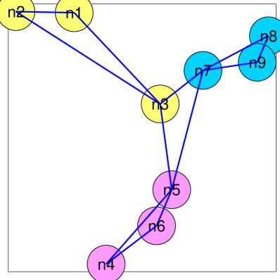
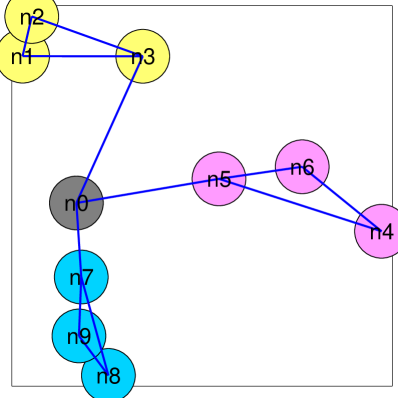
We can express hierarchical connectivity within a OptiGraph by defining a global node that is connected with subgraph nodes. Formulation (2.5) illustrates this idea; this is analogous to (2.4) where we have removed the high level linking constraint (2.4h) and have replaced it with a high level node (2.5h) and three linking constraints that couple the graph to its subgraphs (2.5i). The implementation of the formulation in (2.5) is shown in Code Snippet 3. Here, we assume that we already have graph1, graph2, and graph3 defined from Snippets 1 and 2. We recreate graph0 and setup the node n0 on Lines 2 through 7. We add subgraphs graph1, graph2, and graph3 on Lines 10 through 12 like in the previous snippet, and add linking constraints that connect node n0 to nodes in each subgraph on Lines 15 through 17. We solve the newly created graph0 on Line 20 and present the visualization in Figure 9. This structure is compatible with that shown in Figure 7.
| (Objective) | (2.5a) | ||||
| s.t. | (Subgraph 1 Constraints) | (2.5b) | |||
| (Subgraph 2 Constraints) | (2.5c) | ||||
| (Subgraph 3 Constraints) | (2.5d) | ||||
| (Subgraph 1 Link Constraint) | (2.5e) | ||||
| (Subgraph 2 Link Constraint) | (2.5f) | ||||
| (Subgraph 3 Link Constraint) | (2.5g) | ||||
| (Graph Constraint) | (2.5h) | ||||
| (Global Link Constraints) | (2.5i) | ||||
with three subgraphs.
2.4 Processing and Manipulating OptiGraphs
In addition to the graph construction functions presented in the previous examples (@optinode, @linkconstraint, add_subgraph!), it is also possible to query an OptiGraph object to retrieve its attributes. Table 1 summarizes the main Plasmo.jl functions used to create and inspect an OptiGraph. We inspect the nodes, edges, linking constraints, and subgraphs using getoptinodes, getoptiedges, getlinkconstraints, and getsubgraphs functions, and we can collect all of the corresponding graph attributes using recursive versions of these functions (all_nodes, all_edges, all_linkconstraints and all_subgraphs).
| Function | Description |
|---|---|
| OptiGraph() | Create a new OptiGraph object. |
| @optinode(graph::OptiGraph,expr::Expr) | Create OptiNodes using Julia expression |
| @linkconstraint(graph::OptiGraph,expr::Expr) | Create linking constraint between nodes in graph using expr |
| add_subgraph!(graph::OptiGraph,sg::OptiGraph) | Add subgraph sg to graph |
| getoptinodes(graph::OptiGraph) | Retrieve local OptiNodes in graph |
| getoptiedges(graph::OptiGraph) | Retrieve local OptiEdges in graph |
| getlinkconstraints(graph::OptiGraph) | Retrieve linking constraints in graph |
| getsubgraphs(graph::OptiGraph) | Retrieve subgraphs in graph |
| all_optinodes(graph::OptiGraph) | Retrieve all OptiNodes in graph (including subgraphs) |
| all_optiedges(graph::OptiGraph) | Retrieve OptiEdges in graph (including subgraphs) |
| all_linkconstraints(graph::OptiGraph) | Retrieve all linking constraints in graph (including subgraphs) |
| all_subgraphs(graph::OptiGraph) | Retrieve all subgraphs in graph (including subgraphs) |
Thus far we have discussed how to enable model construction using a bottom-up approach. Specifically, we showed how to construct an OptiGraph by adding subgraphs. We now show how to create an OptiGraph using a top-down approach. Specifically, we show how to partition an OptiGraph, construct subgraphs from the partitions, and use these to derive an alternative representation of the OptiGraph. As part of this, we will discuss how Plasmo.jl interfaces to standard graph partitioning tools.
2.4.1 Hypergraph Partitioning
The OptiGraph is, by default, a hypergraph; as such, we can naturally exploit hypergraph partitioning capabilities. Here, we focus on hypergraph partitioning concepts but we note that our discussion also applies to standard graph partitioning frameworks (a hypergraph can be projected to various standard graph representations). Hypergraph partitioning has received significant interest in the last few years because it naturally represents complex non-pairwise relationships and more accurately captures coupling in such structures compared to traditional graphs. Popular hypergraph partitioning tools include the well-known hMetis and PaToH packages, as well as the comprehensive Zoltan Devine2006 software suite which provides hypergraph partitioning algorithms for C, C++, and Fortran applications. More recent frameworks have made advances to create large-scale hypergraphs Jiang2018 , perform fast hypergraph partitioning Mayer2018HYPEMH , and create high-quality hypergraph partitions shhmss2016alenex .
To provide an overview of hypergraph partitioning techniques, we use notation that is similar to that of an OptiGraph. A hypergraph contains a set of hypernodes and hyperedges where we denote the hypergraph containing hypernodes and hyperedges as . In hypergraph partitioning, one seeks to partition the set of nodes into a collection of at most disjoint subsets such that while minimizing an objective function over the edges such as (2.6a) or (2.6b) subject to a balance constraint (2.6c) (such that partitions are roughly the same size).
| (2.6a) | |||
| (2.6b) | |||
| (2.6c) | |||
Here, and are the most prominent hypergraph partitioning objectives (called the minimum edge-cut and minimum connectivity), where is the set of cut edges of the partitions in (i.e., all edges that cross partitions defined by ). The formulation in (2.6) introduces edge weights for each edge and node sizes for each node which can be used to express specific attributes to the partitioner. For instance, large edge weights typically express tight coupling or high communication volume and nodes sizes often represent computational load. The objective (2.6b) includes the connectivity value which denotes the number of partitions connected by a hyperedge . We also define the parameter in (2.6c) which specifies the maximum imbalance tolerance of the partitions. Lower values of enforce equal-sized partitions and higher values allow for solutions with disparate partition sizes. The lower bound constraint in (2.6c) is not always included in partitioning algorithm implementations.
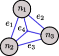
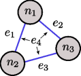
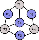
The hypergraph is an intuitive representation for an OptiGraph but other representations are also possible. The hypergraph in Figure 10(a) can be projected to a standard graph representation (shown in Figure 10(b)) or to a bipartite representation (shown in Figure 10(c)). Standard graph representations of optimization problems can utilize mature partitioning tools such as Metis or community detection strategies. This provides flexibility to experiment with different techniques. In the remainder of the discussion we utilize the hypergraph representation for partitioning but we highlight that a broader range of partitioning strategies can be captured in the proposed framework.
2.4.2 OptiGraph Partitioning in Plasmo.jl
Here we discuss partitioning capabilities implemented in Plasmo.jl. Figure 11 depicts the basic aspects of the partitioning framework. We show how to create OptiGraph partitions (with a Partition object), how to formulate subgraphs (with the make_subgraphs! function), and how to combine (aggregate) subgraphs into stand-alone OptiNodes (with the aggregate function). For example, Figure 11(a) contains three partitions ,, and , Figure 11(b) shows the corresponding subgraphs ,, and created from the partitions, and Figure 11(c) depicts the resulting OptiNodes ,, and which represent optimization subproblems. To perform hypergraph partitioning we use the KaHyPar shhmss2016alenex hypergraph partitioner through the KaHyPar.jl interface. KaHyPar targets the creation of high quality partitions and offers a straightforward C library interface which facilitates its connection with Plasmo.jl. Throughout our examples we use the default KaHyPar configuration which uses a direct multilevel k-way algorithm with community detection initialization.
The OptiGraph object offers topology manipulation functionality that can be used, for instance, to modify subgraph structures and formulate subproblems for algorithms. Figure 12 depicts core topology functions we commonly use in the framework. We can query the incident OptiEdges (Figure 12(a)) to a set of OptiNodes (or a subgraph) to inspect coupling (i.e. inspect incident linking constraints). We can also obtain the neighborhood (Figure 12(b)) around a set of OptiNodes to inspect an expanded problem domain, and we can expand (Figure 12(c)) a subgraph into a larger domain and generate the corresponding subproblem.
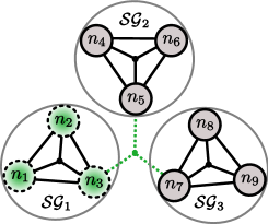
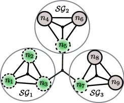
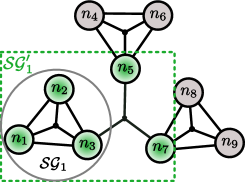
Table 2 summarizes the core graph partitioning and manipulation functions in Plasmo.jl. The gethypergraph function returns a hypergraph object (extends a LightGraphs.jl object) and a reference_map which maps the hypergraph elements back to the OptiGraph (i.e. hypergraph node indices are mapped back to OptiNodes). We also introduce a Partition object that describes how to formulate subgraphs within a graph. As we will show, the Partition object is an intermediate interface to formulate subgraphs in a general way.
| Functions and Descriptions |
|---|
| Create a hypergraph representation of graph. |
| hypergraph,ref = gethypergraph(graph::OptiGraph) |
| Create a Partition given an OptiGraph, a vector of integers and a mapping ref_map. |
| partition = Partition(graph::OptiGraph,vector::Vector{Int},mapping::Dict{Int,OptiNode}) |
| Reform graph into subgraphs using partition. |
| make_subgraphs!(graph::OptiGraph,partition::Partition) |
| Combine subgraphs in graph such that n_levels of subgraphs remain. |
| aggregate(graph::OptiGraph,n_levels::Int) |
| Retrieve incident OptiEdges of OptiNodes in graph. |
| incident_optiedges(graph::OptiGraph,nodes::Vector{OptiNode}) |
| Retrieve neighborhood within distance of nodes. |
| neighborhood(graph::OptiGraph,nodes::Vector{OptiNode},distance::Int) |
| Retrieve a subgraph from graph including neighborhood nodes within distance of sg. |
| expand(graph::OptiGraph,sg::OptiGraph,distance::Int) |
2.4.3 Example 4: Partitioning a Dynamic Optimization Problem
To demonstrate partitioning and manipulation capabilities, we use the simple dynamic optimization problem Shin2018 :
| (2.7a) | ||||
| s.t. | (2.7b) | |||
| (2.7c) | ||||
| (2.7d) | ||||
| (2.7e) | ||||
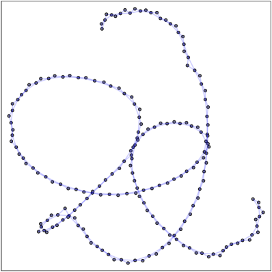
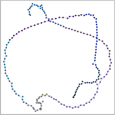
Here, is a vector of states and is a vector of control actions which are both indexed over the set of time indices . Equation (2.7a) minimizes the state trajectory with minimal control effort (energy), (2.7b) describes the state dynamics, and (2.7c) is the initial condition. This problem can be formulated using an OptiGraph as shown in Code Snippet 4 in much the same way as the examples in Section 2.3. We define the number of time periods and create a disturbance vector d (data) on Lines 1 through 6. In our implementation we create separate sets of nodes for the states and controls on Lines 12 and 13, but it is also possible to define nodes for each individual time interval and add state and control variables to the resulting nodes. Having control over this granularity is convenient for expressing what can be partitioned (i.e. features defined in an OptiNode will remain in the same partition). Next we setup the state and control OptiNodes on Lines 16 through 31, we use a linking constraint to capture dynamic coupling on Line 34 and we show how to solve the problem with Ipopt Wachter2006 on Line 39. We visualize the graph topology and matrix in Figure 13. The layouts depict a linear graph but we note that the matrix has no obvious structure.
optimization problem.
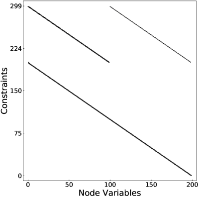
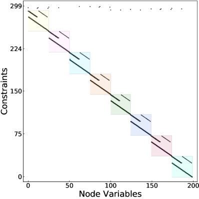
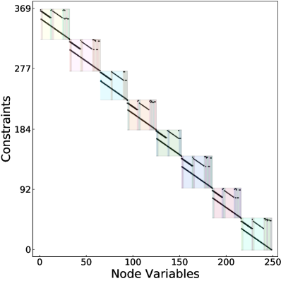
We partition the graph using KaHyPar, as shown in Code Snippet 5; here, Line 2 imports the KaHyPar interface and Line 5 creates the hypergraph representation corresponding to the OptiGraph using gethypergraph. We also return a reference_map which maps the hypergraph elements back to the OptiGraph. Line 8 performs hypergraph partitioning using KaHyPar with a maximum imbalance () of 10% and Line 11 creates a Partition object using the resulting partition vector and the reference_map. Line 14 creates subgraphs in the graph graph using the Partition object and the make_subgraphs! function. We visualize the topology and matrix of the partitioned problem on Lines 16 and 19 and these are shown in Figure 14. This reveals eight distinct partitions and their corresponding coupling. We note that the partitions are well-balanced and note that the matrix is now rearranged into a banded structure that is typical of dynamic optimization problems (partitioning automatically induces reordering). Plasmo.jl can use other graph representations to perform partitioning. For instance, we can create a traditional graph representation, as shown in Code Snippet 6, and partition it with Metis. We then use the reference_map to obtain the original OptiGraph elements to create a graph Partition. We could also partition less intuitive representations (e.g., bipartite) in this way; we only require a mapping from the partition back to the OptiGraph elements. The partitioning procedure shown here can also be repeated to create an arbitrary number of subgraph levels.
optimization problem.
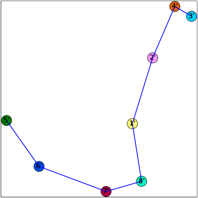
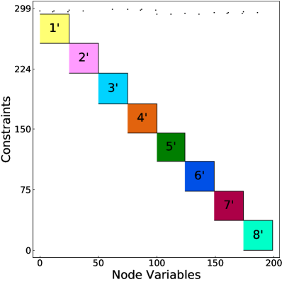
The OptiNodes in a graph can be aggregated to form larger nodes, as shown in Figure 11(c). This aggregation functionality is key to communicate subproblems to decomposition algorithms that operate at different levels of granularity. Aggregation can also be performed to collapse an entire graph into a single node, producing a standard optimization problem that can be solved with off-the-shelf solvers. Code Snippet 7 shows how to aggregate the graph of the dynamic optimization problem into a new aggregated graph with eight nodes. We create the new (aggregated_graph) on Line 2 by using aggregate on the graph from Snippet 5. We provide the integer 0 to the function to specify that we want zero subgraph levels which converts the eight subgraphs into nodes. For hierarchical graphs with many levels, we can define how many subgraph levels we wish to retain. We plot the graph and matrix layouts for the aggregated OptiGraph on Lines 5 and 8 and these are shown in Figure 15.
optimization problem.
2.4.4 Example 5: Using Graph Topology Functions
We now show how to use graph topology functions by computing overlapping partitions for the dynamic optimization example. This is shown in Code Snippet 8; here, Line 2 obtains subgraphs from the OptiGraph graph created in Snippet 5, Line 8 determines and returns the OptiEdges incident to the OptiNodes in the first subgraph sg1, and Line 12 returns the complete neighborhood around the same OptiNodes within a distance of two. On Line 16, we broadcast the expand function (using dot syntax expand.() and Ref as typical in Julia) to create a new set of subgraphs, each expanded by a distance of two. Line 19 plots the layout of graph with the expanded subgraphs as is shown in Figure 16. Here, we see eight distinct partitions (each with a unique color) where the larger markers represent nodes that are part of multiple subgraphs (they are also the average color of their containing subgraphs). Figure 16 shows the corresponding matrix layout where highlighted columns indicate that the node also appears in other subgraph blocks. Overlapping partitions are useful in certain algorithms such as Schwarz decomposition.
3 Algorithms
The OptiGraph provides a flexible abstraction that facilitates communication of problem structure to a wide range of decomposition strategies. The structure can be exploited at a problem level, in which the decomposition strategy treats OptiNodes as optimization subproblems whose solutions are coordinated to find a solution of the entire OptiGraph. This strategy is used, for example, in Benders, Lagrangian dual, and ADMM decomposition. The structure can also be exploited at the linear algebra level, in which a decomposition strategy is used within a general algorithm to compute a search step. Here, the strategy treats OptiNodes as linear systems that result from the optimality conditions of the associated subproblems and coordinates their solutions to find a solution of the linear system associated with the optimality conditions of the entire OptiGraph. In this section we show how to use the proposed abstraction and Plasmo.jl functionality to explain structures at the linear algebra and problem level.
3.1 Linear Algebra Decomposition
It is well-known that block structures can be exploited by linear algebra operations within interior-point algorithms. For instance, continuous problems with the partially-separable structure described by (2.1) induce structured linear algebra kernels that can be solved using tailored techniques such as Schur decomposition. We express the continuous variant of the graph formulation (2.1) with feasible sets of the form which gives rise to the Karush-Kuhn-Tucker (KKT) system given by:
| (3.8a) | |||
| (3.8b) | |||
| (3.8c) | |||
Here, we recall that denotes the nodes that support edge . The terms associated with barrier functions exist in (3.8) in the presence of inequality constraints. Upon linearization of (3.8), the system of algebraic equations gives rise to the block-bordered KKT system given by:
| (3.24) |
Here, is the primal-dual step for the variables and constraints on node and is a vector of steps corresponding to the dual variables on the OptiEdges in OptiGraph , where . We also define
as the block matrix corresponding to OptiNode where is the Hessian of the Lagrange function of (2.1) and is the constraint Jacobian. We define coupling blocks as
where . If all of the linking constraints in the graph are linear, reduces to where is the matrix of coefficients corresponding to the OptiEdges incident to node .
3.1.1 Schur Decomposition
The block-bordered structure described in (3.8) can be exploited using Schur decomposition or block preconditioning strategies. The typical Schur decomposition algorithm is described by (3.25) in terms of the OptiGraph abstraction, where is the Schur complement matrix.
| (3.25a) | |||
| (3.25b) | |||
| (3.25c) | |||
Step (3.25a) requires factorizing the linear system associated to each OptiNode () and computes the Schur complement contribution on each node (possibly in parallel). After each contribution is computed (each requires performing a sparse factorization), the total Schur complement matrix is created and factorized to solve the linear system (3.25b) (in serial) and take a step in the OptiEdge dual variables (). Step (3.25c) solves for the OptiNode primal-dual step given the OptiEdge dual step (also possibly in parallel).
The general Schur decomposition exhibits a couple of major computational bottlenecks. Forming the contributions is expensive when there are many columns in (the number of columns corresponds to the number linking constraints incident to node ). Moreover, if the node blocks have different sizes, the factorization of the blocks can create load imbalance and memory issues. Second, factorizing the Schur matrix is challenging when there are many linking constraints because this matrix is dense or is composed of dense sub-blocks. Consequently, one needs to control the amount of coupling between the blocks. The OptiGraph topology directly corresponds with the size of the block matrices that appear in the Schur decomposition and thus can be manipulated to facilitate computational efficiency. Specifically, we wish to manipulate the partitioning of an OptiGraph to accelerate Schur decomposition. We use the capabilities of Plasmo.jl to experiment with different partitioning strategies and with this analyze trade-offs between coupling, imbalance, and memory use. Section 4.1 details these performance trade-offs with a large example.
3.1.2 PIPS-NLP Interface
Plasmo.jl includes an interface to the structure-exploiting interior-point solver PIPS-NLP that we call
PipsSolver.jl.
PIPS-NLP provides a general Schur decomposition strategy that performs parallel computations via MPI. PIPS-NLP was developed to solve large-scale stochastic programming problems
that adhere to a two-level tree structure (i.e. a single first stage problem coupled to second stage subproblems).
The OptiGraph interface to PIPS-NLP converts general graph structures into this format (e.g., via aggregation and partitioning). For instance, using
our example problem (2.7), we can communicate the problem structure to PIPS-NLP
and solve the problem in parallel. This is shown in Snippet 9.
Snippet 9 presents a standard template for setting up distributed computing environments to use PipsSolver.jl which is worth discussing. Line 1 imports the Distributed module, which is a Julia package for performing distributed computing. On Line 2 we import the MPIClusterManagers package which allows us to interface MPI ranks (used by PIPS-NLP) with Julia worker CPUs. We create a manager object and specify that we want to use 2 workers on Line 5 and add the Julia workers on Line 7. Next we setup the model and solver environments for the added workers on Lines 10 and 11 and create a reference to the julia workers by querying the manager on Line 14. We distribute the graph among the workers in Line 18 using the function provided by PipsSolver. This function sets up the relevant graph nodes on each worker and creates the graph named pips_graph on each worker (internally this function inspects the OptiGraph and allocates OptiNodes to worker CPUs). Finally, we use the mpi_do function from MPIClusterManagers to execute MPI on each worker and solve the graph. Each worker executes the pipnlp_solve function and communicates using MPI routines within PIPS-NLP.
3.2 Problem Level Decomposition
Overlapping Schwarz is a flexible graph-based decomposition strategy that can be used at the linear algebra or problem level Fromeer2002 ; Shin2020 . This approach has been used to solve dynamic optimization Shin2019 and network optimization problems Shin2020b . At the problem level, the Schwarz algorithm decomposes the problem graph over overlapping partitions. The algorithm solves subproblems over the overlapping partitions and coordinates solutions by exchanging primal-dual information over the overlapping regions. The presence of overlap is key to promote convergence; in particular, it has been proven that the convergence rate improves exponentially with the size of the overlap Shin2020 . The Schwarz scheme is also flexible in that the overlap can be adjusted to trade-off subproblem complexity (time and memory) with convergence speed. When the overlap is the entire graph, the algorithm solves the entire graph once (converges in one iteration). When the overlap is zero, the algorithm operates as a standard Gauss-Seidel scheme and will exhibit slow convergence (or no convergence at all). We thus have that Schwarz has fully centralized and fully decentralized schemes as extremes. Schwarz algorithms can also be implemented under synchronous and asynchronous settings to handle load imbalance issues Shin2020 .
3.2.1 Development of Schwarz Algorithm
The Schwarz algorithm iteratively solves subproblems associated with overlapping subgraphs. In particular, one first constructs expanded subgraphs from the subgraphs obtained from OptiGraph partitioning. This procedure can be performed by expanding the subgraphs and adding OptiNodes within a prescribed distance . The optimization subproblems for the expanded subgraph can be formulated as:
| (3.26a) | ||||
| s.t. | (3.26b) | |||
| (3.26c) | ||||
| (3.26d) | ||||
Here, the dual variables for (3.26c) and (3.26d) are denoted by , is the set of nodes in subgraph , and the superscript denotes the itertion counter. For representation we denote and as two separate sets of incident edges where . More specifically, is the set of edges incident to (i.e. edges that contain a node in another subgraph) and and denote how the incident linking constraints are formulated within the subproblem using either primal or dual coupling.
In our formulation, (3.26a) is the subproblem objective which is the sum of node objective functions contained in the expanded subgraph where we have added the dual penalties from the incident dual linking constraints on edges , and (3.26d) represents primal constraints we have added from the edges . Note that incident linking constraints can be directly incorporated into the subproblem as local constraints, or included in the objective function as a dual penalty (this assigning procedure can be important to the algorithm performance). In our implementation, one may provide preference on whether a linking constraint is treated in primal or dual form (we show in Section 4.2 how to do this). The primal-dual solution of the other subproblems obtained from the previous iteration, in particular and , also enter into the subproblem formulation. The Schwarz algorithm achieves convergence with this exchange of information.
An important step in the Schwarz algorithm is the restriction of the subproblem solution. One obtains the primal-dual solution and by solving (3.26). We observe that the solutions from different subproblems overlap (the solution for overlapping nodes may appear more than once). We thus use a restriction step to eliminate such multiplicity; in particular, we discard the part of the solution associated with the nodes that are acquired by expansion. The restriction step can be expressed as:
The solution of subproblems can be performed in parallel. Next, the primal-dual residual at any Schwarz iteration is evaluated according to the residual to the KKT system for (3.27). We define as the primal residual of the linking constraints on edge at iteration , and as the dual residual of the linking constraints on edge . Specifically, the primal error evaluates the linking constraints in the higher level graph , and the dual error evaluates the consensus of the dual values of the expanded subgraphs that contain the edge ; for the case where more than two subgraphs are associated with one linking constraint, see (Shin2020b, , Proposition 1) for details on how to evaluate dual infeasiblility. The formal definition of these residuals is given by:
| (3.27a) | |||
| (3.27b) | |||
The termination criteria can be set as follows:
| (3.28) |
where is the prescribed convergence tolerance.
The Schwarz algorithm can be expressed using syntax that closely matches that of the
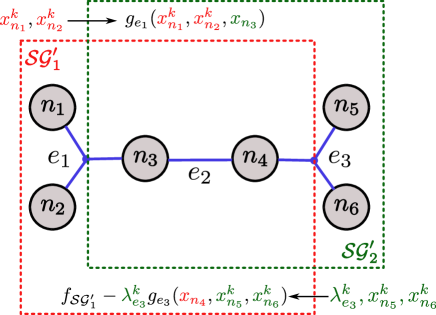
OptiGraph abstraction, as shown in Algorithm 1.
Figure 18 depicts how
primal-dual information is exchanged in the overlapping subgraph scheme.
The figure also depicts a simple graph that contains two subgraphs and and one edge
that connects the subgraphs ().
The right side of Figure 18 shows the expanded subgraphs and
. In this illustration, edge is incident to subgraph and communicates primal
information (i.e. it is in the set ), and edge is incident to subgraph
and communicates dual information to subgraph (i.e. it is in the set ).
3.2.2 Implementation of Schwarz Algorithm
We implemented the Schwarz algorithm in Plasmo.jl and call this SchwarzSolver.jl. Code Snippet 10 shows how we can solve the overlapping subgraphs we produced in Code Snippet 8 corresponding to the overlap shown in Figure 16. On Line 1 we import the Schwarz solver, on Line 5 we create an Ipopt optimizer to use as the subproblem solver, and we execute the algorithm on Line 8. It is also possible to pass an overlap distance instead of the expanded subgraphs and allow the Schwarz solver to perform the subgraph expansion. The benefit of formulating subgraphs at the user level is that one could formulate custom overlap schemes.
4 Case Studies
We demonstrate modeling and solution capabilities enabled by the OptiGraph abstraction and the Plasmo.jl implementation using a couple of challenging problems arising in infrastructure networks. The implementations used for the case studies can be found at https://github.com/zavalab/JuliaBox/tree/master/PlasmoExamples. We highlight that the study presented in Section 4.1 uses a dataset that cannot be shared (we only present computational results to demonstrate scalability). In the GitHub repository we provide a simple network dataset that uses the same features of Plasmo.jl.
4.1 Linear Algebra Decomposition of a Natural Gas Network
We solve a large dynamic optimization problem for the natural gas network shown in Figure 1(a). This network includes four gas supplies, 153 time-varying gas demands, 215 pipelines, and 16 compressor stations. The goal of the optimization problem is to track demands and minimize compressor power over a 24-hour time horizon. The main complexity of this problem arises from nonlinear PDEs needed to capture conservation of mass and momentum inside the pipelines. After space-time discretization of the PDE, we obtain a nonconvex NLP with 432,048 variables, 427,512 equality constraints, and 3,887 inequality constraints. Figure 2(b) depicts the graph structure induced by the space-time nature of this problem. Our goal is to identify efficient partitions that traverse space-time to efficiently solve the problem using Schur decomposition in PIPS-NLP.
All model details can be found in Zavala2014 and Jalving2018 and in the scripts provided with this work. Here we provide a summary to showcase modeling features of Plasmo.jl. The gas network contains links and junctions . The set of junctions connect links and include gas supplies (injections) and demands (withdrawals) . The set of links is composed of both pipeline links and compressor links such that . We also specify the set of time periods as with a 24-hour horizon and . For our implementation, each component of the system is modeled as a stand-alone OptiGraph with OptiNodes distributed over time and we connect these in a high-level graph to form the complete problem. This modular construction is one of the benefits of the graph abstraction. Specifically, component models can be developed separately (e.g., by different people). Moreover, the syntax of the different components can be different because each OptiGraph is a self-contained object. This greatly facilitates model construction and debugging. This differs from standard algebraic modeling languages, in which the syntax in the entire model has to be compatible (this complicates debugging of large models). The implementations to construct each component model (each OptiGraph) in Plasmo.jl can be found in the Appendix.
Junction OptiGraph
The gas junction model is described by (4.29), where is the pressure at junction
and time interval . is the lower pressure bound for the
junction, is the upper pressure bound, is the target demand flow for demand on junction
and is the available gas generation from supply on junction .
Code Snippet 13 in the Appendix shows how to create the junction graph.
| (4.29a) | |||
| (4.29b) | |||
| (4.29c) | |||
Pipeline OptiGraph
Each pipeline model is an OptiGraph with OptiNodes distributed on a space-time grid. Specifically, the nodes of each pipeline graph form a mesh
wherein pressure and flow variables are assigned to each node. Flow dynamics within pipelines are expressed with linking constraints that describe the discretized
PDE equations for mass and momentum using finite differences. We assume isothermal flow through each horizontal pipeline segment which are
described by the conservation equations from Osiadacz1984 . The pipeline formulation is given by (4.30)
where and are the pipeline pressure and flow for each pipeline link at each time period for each
space point where is the set of spatial discretization points we use for each pipeline.
We also define for convenience.
The constants given in this formulation for each pipeline are , ,
and . Here, the pipeline terms are the cross-sectional
area , diameter , friction coefficient ,
the gas speed of sound squared , and the scaling coefficient . We denote expressions for
the flow in and out of each pipeline at each time as and as well as the total line pack (inventory of gas)
in each pipeline link at each time as . With the defined terms,
(4.30a) and (4.30b) are the mass and momentum equations, (4.30c), (4.30d), (4.30e), (4.30f)
define the convenience variables for flow and pressure in and out of each pipeline, (4.30g) and (4.30h)
prescribe the system to initially be at steady-state, and (4.30i) and (4.30j) define line pack and require
each pipeline to refill its line pack by the end of the time horizon.
Capturing the space-time structure of (4.30) is seemingly complex but it is straightforward to do so with an OptiGraph because each pipeline can be treated independently. Code Snippet 14 in the Appendix details how each pipeline model is constructed.
| (4.30a) | |||
| (4.30b) | |||
| (4.30c) | |||
| (4.30d) | |||
| (4.30e) | |||
| (4.30f) | |||
| (4.30g) | |||
| (4.30h) | |||
| (4.30i) | |||
| (4.30j) | |||
Compressor OptiGraph
The compressor models are created analogously to the junction and pipeline models. We use an ideal isentropic formulation given by
(4.31) where , , , and are the compression ratio,
suction presure, discharge pressure, and horsepower respectively for compressor link at time . We also define
constant parameters, , , and for heat capacity, temperature and isentropic efficiency. The variables
and are used for convenience to be consistent with the pipeline link formulation.
The compressor graph construction is straightforward and is shown in Code Snippet 15 in the Appendix.
| (4.31a) | |||
| (4.31b) | |||
| (4.31c) | |||
Network OptiGraph
The network structure of the model is induced using a high-level graph wherein we use linking constraints
to express mass conservation around each junction and boundary conditions for pipeline and compressor links according
to the formulation given by (4.32). Here, (4.32a) represents mass conservation
at each junction and (4.32b) and (4.32c) are the pipeline and compressor link boundary conditions. We also
define and as the receiving and sending junction for each link at time
and we define and as the set of receiving and sending links to each junction respectively.
The final optimal control problem is given by (4.33) which seeks to minimize the total operating cost over
the 24-hour period where is the compressor cost for compressor link and is the gas delivery price for demand on junction .
The complete formulation includes all of the junction, pipeline, compressor, and network equations.
Code Snippet 16 in the Appendix assembles the complete natural gas model.
| (4.32a) | |||
| (4.32b) | |||
| (4.32c) | |||
| (4.33a) | |||||
| Junction Limits | (4.33b) | ||||
| Pipeline Dynamics | (4.33c) | ||||
| Compressor Equations | (4.33d) | ||||
| Network Link Equations | (4.33e) | ||||
Partitioning and Solving the Natural Gas Problem
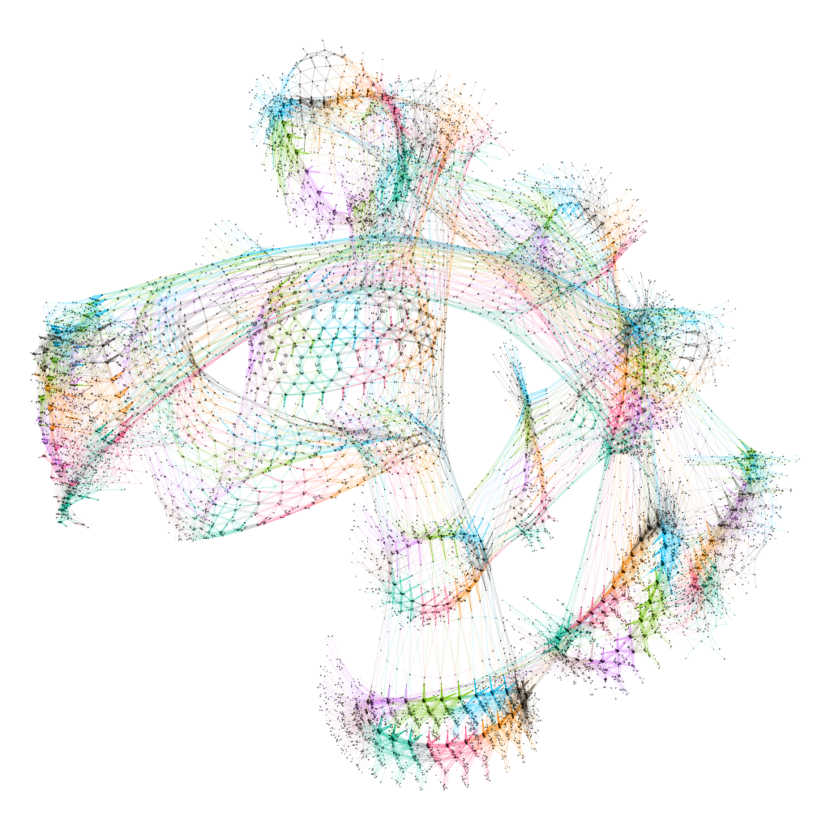
Once we have constructed a graph representation of the problem, we can use the Plasmo.jl tools to explore different partitioning strategies. Figure 19 visualizes the graph structure of the problem and shows different partitions. Figure 19(a) shows the graph components we assembled in the above snippets with pipeline nodes depicted in grey, compressor nodes in green, and junctions in blue. Figure 19(b) depicts a pure time partition of the problem with 8 partitions (each with a different color). Partitioning in time is an intuitive approach but this results in 87,505 linking constraints (making the Schur matrix intractable). This problem can also be partitioned purely as a network wherein we consider the partition of the network components themselves (as opposed to the structure of the problem) which is shown in Figure 19(c). The network partition is physically intuitive but it does not capture the true mathematical structure of the problem nor consider load balancing. We highlight that both time and network partitioning approaches can be performed using the partitioning framework (by manually defining a partition vector), but the value of having the graph is that we can efficiently obtain space-time partitions to produce the partition shown in Figure 19(d). While visually similar to the network partition, the space-time partition produces considerably less coupling (748 linking constraints against 1,800 linking constraints), thus leading to a small Schur matrix. We also highlight that the space-time partition requires traversing space-time.
Code Snippet 11 shows how to partition the gas network problem and produce the problem we communicate to PIPS-NLP. Line 2 imports the KaHyPar hypergraph partitioner, Line 5 formulates the hypergraph representation of our problem, and Lines 8 through 10 setup weight vectors we use for the nodes and edges (we weight nodes by their number of variables and edges by their number of linking constraints). We partition the hypergraph on Line 14, create a Partition object on Line 17, produce new subgraphs on Line 20 and finally aggregate the subgraphs on Line 23.
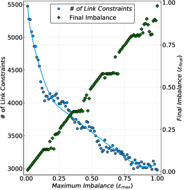
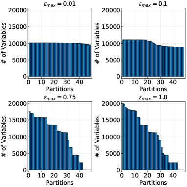
The partitioning in Snippet 11 produces a graph with 8 nodes which we can distribute and solve with PIPS-NLP. We follow the exact same setup used in Snippet 9 using PipsSolver.jl and distribute the graph between workers to solve in parallel on a machine with 32 Intel Xeon CPUs E5-2698 v3 running at 2.30 GHz. We experiment with different numbers of partitions and imbalance values and explore how the PIPS-NLP algorithm performs. Table 3 details the results obtained where we vary the number of partitions (8, 24, and 48) and the maximum imbalance value (between 0.01 and 1.0). Figure 20 shows the effect of increasing the imbalance for the 48 partition case on the true final imbalance the partitioner produced () and the total number of linking constraints. For the most part, the maximum and final imbalances display a one-to-one relationship but there are distinct intervals wherein the final imbalance flattens out. We also see that nominal values of maximum imbalance (less than 25%) reduce the number of linking constraints considerably but greater values produce diminishing returns. Here, we also show the distribution of subproblem sizes for a few select maximum imbalance values on the right side of Figure 20 for reference. We can see that, under naive partitioning, the size of the partitions can vary by an order of magnitude.
For each run, we note the true imbalance KaHyPar produced , the sum of the edge weights (which
corresponds to the number of linking constraints), the maximum node size
(which corresponds to the node
with the most variables), as well as the average and maximum
number of node connections (i.e. the number of linking constraints incident to a node). For timing results we observe the time spent building the KKT system (i.e.
the time to build (3.25b)),
the time spent factorizing the
Schur complement (i.e. time to solve (3.25b)) and the total time spent inside PIPS-NLP .
The first rows of Table 3 show results with 8 partitions and also include cases for time and network partitions corresponding
to Figures 19(b) and 19(c). As expected, the high degree of coupling in these partitions is
computationally prohibitive; the time partition cannot be solved with Schur complement decomposition and the network partition requires over 2 hours.
Significant improvement is achieved by using the KaHyPar partitioner; we note that even a 1% imbalance is twice as fast as the network partition.
Increasing the imbalance parameter to 50% results in much better performance (the average and maximum number of columns in decreases), but increasing it to 60% results in
diminished speed, despite producing a similar partition. Interestingly, allowing too much imbalance can result in
ill-conditioned subproblems (e.g., ill-conditioned matrices ). This highlights why having flexibility in partitioning is important. The second and third sets of rows present the
results using 24 and 48 partitions with 24 CPUs. Increasing the maximum imbalance
for the 24 partition case results in diminished performance (due to the bottleneck of building the KKT system). This is because either the node connectivity
increases (for the 10% imbalance),
the maximum subproblem size increases (for the 100% imbalance), or there is some ill-conditioning of the subproblems. In contrast, increasing the imbalance for the 48 partition case results in
computational improvement. This is because more linking constraints (more coupling) shifts the bottleneck step to
factorizing the Schur complement and drastic speedups result from reducing the degree of coupling. This highlights how flexible partitions can help fit the solver to the computing architecture of interest.
| Partition |
|
|
|
|
|
|
|||||||||||||||
| = 8 # Proc = 8 | time | 0.0 | 87505 | 60567 | 21877 , 24940 | - | - | - | |||||||||||||
| network | 0.41 | 1800 | 85248 | 459 , 1368 | 7236 | 56 | 7505 | ||||||||||||||
| 0.01 | 0.0073 | 748 | 61008 | 205 , 316 | 2944 | 6.3 | 3115 | ||||||||||||||
| 0.5 | 0.37 | 434 | 83202 | 121 , 218 | 2269 | 1.7 | 2475 | ||||||||||||||
| 0.6 | 0.37 | 458 | 83202 | 124 , 218 | 2862 | 1.9 | 3069 | ||||||||||||||
| = 24 # Proc = 24 | 0.01 | 0.01 | 2889 | 20390 | 259 , 431 | 1746 | 273 | 2117 | |||||||||||||
| 0.1 | 0.1 | 2748 | 22200 | 256 , 529 | 1934 | 236 | 2270 | ||||||||||||||
| 1.0 | 0.99 | 1572 | 40080 | 127 , 362 | 2279 | 54 | 2447 | ||||||||||||||
| = 48 # Proc = 24 | 0.01 | 0.01 | 5472 | 10194 | 245 , 482 | 2029 | 1769 | 3954 | |||||||||||||
| 0.1 | 0.1 | 4560 | 11104 | 210 , 440 | 1871 | 1031 | 3054 | ||||||||||||||
| 0.75 | 0.75 | 3182 | 17642 | 151 , 387 | 2126 | 368 | 2670 | ||||||||||||||
| 1.0 | 0.98 | 2978 | 19985 | 143 , 480 | 1826 | 298 | 2247 |
4.2 Overlapping Schwarz Decomposition for DC OPF
This case study demonstrates how we can use graph partitioning and topology manipulation to pose a complex power network problem to the Schwarz overlapping scheme. We consider a 9,241 bus test case obtained from pglib-opf (v19.05) pglib , which we obtain through Power-Models.jl powermodels . We denote the power grid as a network containing a set of electric buses that connect power lines . Each electric bus can include generators and serves a total power load . The total set of generators is given by such that . The network is described by the DC power flow equations Sun2018 given by (4.34) where (4.34a) seeks to minimize the total generation cost and voltage angle difference where is a regularization parameter. (4.34b) enforces energy conservation, and (4.34e) and (4.34f) denote limits on power generation and voltage angles. In this formulation, is the bus voltage angle for each bus , is the power generation from generator with cost coefficients and and lower and upper limits and , and and are the inlet and outlet voltage angles on with ramp limit . We also define as the set of power links received by bus and as the set of links sent from bus . The power flow on line is defined by (4.34d), where is the branch admittance for line , is the source bus voltage angle and is the destination bus voltage angle. denotes the source bus of line and is destination bus for line . We denote the voltage angles on the set of reference buses in (4.34g) where is the set of reference buses.
| (4.34a) | ||||
| (4.34b) | ||||
| (4.34c) | ||||
| (4.34d) | ||||
| (4.34e) | ||||
| (4.34f) | ||||
| (4.34g) | ||||
We construct the DC OPF model with Code Snippet 17, which produces an optimization problem with over 100,000 variables and constraints. The DC OPF model is partitioned using KaHyPar; once we obtain partitions, we create subgraphs, expand them, and solve the problem using the SchwarzSolver.jl. Code Snippet 12 demonstrates how we carry this out using a maximum imbalance of 10% and an overlap size of . Line 1 imports KaHyPar and Line 6 creates a hypergraph and ref_map which we use for partitioning. Lines 9 through 11 query the graph for edge weights and node sizes, Line 15 partitions the DC OPF problem, and Lines 18 and 21 create a Partition and use it to define subgraphs for the problem. Once we have subgraphs, we perform a subgraph expansion on Line 27 and execute the Schwarz solver on Line 31. We also show how to tell the solver how to treat linking constraints. We provide the keyword argument primal_links with the vector of power flow linking constraints and we provide the keyword dual_links with a vector of voltage angle linking constraints to denote how subproblems are formulated; the constraints that are specified as primal_links are treated as direct constraints while the constraints in dual_links are incorporated as dual penalty as described in (3.26).
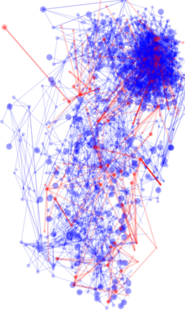
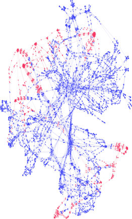
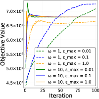
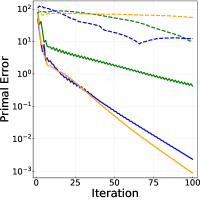
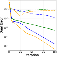
Figure 21 depicts the original and overlapping partitions obtained from Snippet 12. These are visualized using Gephi. We experiment with different values for maximum imbalance and overlap and obtain the results in Figure 22. We see that the Schwarz algorithm fails to converge with an overlap value of one (for any imbalance value) which is consistent with the convergence analysis in Shin2020b , but a sufficient overlap of 10 produces smooth convergence (for each imbalance value). We also found that larger partition imbalance results in faster convergence (with sufficient overlap) which is likely due to the smaller edge cut and fewer linking constraints that need to be satisfied. We thus see that the trade-offs of imbalance and coupling are complex and differ under different problems and algorithms.
5 Outlook and Extensions for Plasmo.jl
We presented a graph-based modeling abstraction for optimization that we call an OptiGraph. We showcased its implementation in Plasmo.jl and demonstrated how this provides flexibility to use different graph analysis and visualization tools. We also showed how these capabilities facilitate the use of decomposition strategies at both the linear algebra and problem levels. There are broad opportunities to refine and expand the capabilities of the proposed abstraction and of Plasmo.jl. The most evident next step is to develop interfaces to a wider range of decomposition solvers. As such, we are currently developing interfaces to DSP Kim2016 (a Benders and Lagrangian dual decomposition solver for stochastic optimization), and SNGO Cao2019 (a Julia-based global solver for nonlinear stochastic programs). We are also interested in new parallel interior point solvers that use recent Schur decomposition strategies to solve massive energy system models Onheit2019 . In this regard, the graph could be a natural interface for BELTISTOS Kourounis2019 , a nonlinear solver that exploits specialized time decomposition structures that arise in Schur decomposition. These capabilities will enable solution of a wide range of application problems.
As ongoing work we are also developing parallel modeling capabilities to create graph objects in parallel. Parallel modeling becomes important in instances when the model itself is too large to fit in memory, such as with stochastic programs with many scenarios. Scenario-based optimization problems have been modeled in parallel using StructJuMP and MPI, but more complex structures (such as those with many linking constraints) are more challenging to implement in a parallel modeling framework. In this context, the Parallel Structured Model Generator (PSMG) Qiang2014 is the only framework we know of that performs parallel model generation which works with structured conveying modeling language (SML) Colombo2009 . PSMG focuses on efficient distributed memory design to achieve parallel generation, but it requires solvers to perform subproblem distribution and load balancing based on a well-defined model structure. In contrast, we hope to facilitate the modeling, partitioning, and parallel generation tasks in a more systematic interactive framework using the OptiGraph.
Finally, we demonstrated how to partition graphs using powerful tools such as Metis and KaHyPar. Exploiting such graph partitioning tools opens many possibilities for using decomposition - based solvers, but it is limited to expressing problem characteristics strictly in the form of edge weights and node sizes. We are interested in developing more customized graph partitioning algorithms that work directly on the graph attributes (such as accounting for integer variables). We are also interested in developing algorithms that calculate overlap directly as opposed to performing subgraph expansion. Such modeling advances can provide new capabilities that open diverse algorithmic development and offer interesting directions for future research.
Acknowledgements
This material is based on work supported by the U.S. Department of Energy (DOE), Office of Science, under Contract No. DE-AC02-06CH11357 as well as the DOE Office of Electricity Delivery and Energy Reliability’s Advanced Grid Research and Development program (AGR&D). This work was also partially supported by the U.S. Department of Energy grant DE-SC0014114. We also acknowledge partial support from the National Science Foundation under award NSF-EECS-1609183. The authors acknowledge Yankai Cao for his work developing the original PIPS-NLP interface for Plasmo.jl. The authors also acknowledge Michel Schanen from Argonne National Laboratory for his assistance using and debugging PIPS-NLP as well as Kibaek Kim from Argonne National Laboratory for his help in the conceptualization of Plasmo.jl.
Appendix: Code Snippets
Junction OptiGraph Implementation
The junction OptiGraph is implemented in Code Snippet 13.
We define the function create_junction_model on Line 2 which accepts junction specific data and the number of time
periods nt. We create the OptiGraph graph on Lines 3 through 26 where
we add a node for each time interval and then create the variables and constraints for each node in a loop. We also use the JuMP specific
@expression macro to refer to expressions for total gas supplied, total gas delivered, and total cost for convenience. The junction model
is returned from the function on Line 29.
Pipeline OptiGraph Implementation
The pipeline OptiGraph is given by Code Snippet 14.
We again use a function (create_pipeline_model) to create the graph
and we unpack the input data and create nodes, variables, and constraints on Lines 3 through 25.
We define the set of OptiNodes on Line 10 as grid, which we use to refer to OptiNodes using time and space indices.
To capture the space-time coupling of each pipeline we use linking constraints on Lines 28 through
42 to define the finite difference scheme, the steady-state condition, and the line pack constraint.
Compressor OptiGraph Implementation
The compressor OptiGraph construction is fairly straight-forward and given by
15. Line 1
defines the function
create_compressor_model which takes data and the number of time periods nt.
Line 3 creates the OptiGraph for the compressor model, Line 4
creates an OptiNode for each time point, and Lines 7 through 15 define the model variables
and constraints. Lines 19 and 20 define helpful expressions for the flow in and out of the compressor and Line 23
returns the OptiGraph.
Network OptiGraph Implementation
The network OptiGraph couples the other component graphs at a higher level and is implemented in Code Snippet 16.
We create the graph gas_network on Line 2 and add the component subgraphs
on Lines 5 through 13.
Once we have the multi-level subgraph structure we create linking constraints at the gas_network level on Lines
16 through 46 which impose the junction conservation and
boundary conditions for the network links (pipelines and compressors).
DC OPF Model Implementation
The DC optimal power flow model is implemented in Code Snippet 17.
Line 1 loads the bus system using PowerModels.jl, Line 4 creates the graph,
Lines 7 and 8 create nodes
for each bus and line in the network, and Line 11 assigns relevant data to each bus and line node using a load_data! function. The
DC OPF model is constructed in the same fashion as described in earlier examples where Lines 14 through 55
setup models on each node and add linking constraints corresponding to power conservation and voltage angle connections.
References
- (1) Abhyankar, S., Brown, J., Constantinescu, E. M., Ghosh, D., Smith, B. F., and Zhang, H. Petsc/ts: A modern scalable ode/dae solver library. arXiv preprint arXiv:1806.01437 (2018).
- (2) Allman, A., Tang, W., and Daoutidis, P. Towards a Generic Algorithm for Identifying High-Quality Decompositions of Optimization Problems. In Computer Aided Chemical Engineering. 2018.
- (3) Allman, A., Tang, W., and Daoutidis, P. Decode: a community-based algorithm for generating high-quality decompositions of optimization problems. Optimization and Engineering (06 2019).
- (4) Babaeinejadsarookolaee, S., Birchfield, A., Christie, R. D., Coffrin, C., DeMarco, C., Diao, R., Ferris, M., Fliscounakis, S., Greene, S., Huang, R., Josz, C., Korab, R., Lesieutre, B., Maeght, J., Molzahn, D. K., Overbye, T. J., Panciatici, P., Park, B., Snodgrass, J., and Zimmerman, R. The power grid library for benchmarking ac optimal power flow algorithms, 2019.
- (5) Bastian, M., Heymann, S., and Jacomy, M. Gephi: An open source software for exploring and manipulating networks, 2009.
- (6) Bergner, M., Caprara, A., Ceselli, A., Furini, F., Lübbecke, M. E., Malaguti, E., and Traversi, E. Automatic dantzig–wolfe reformulation of mixed integer programs. Mathematical Programming 149, 1 (feb 2015), 391–424.
- (7) Biel, M., and Johansson, M. Efficient stochastic programming in julia, 2019.
- (8) Boyd, S., Parikh, N., Chu, E., Peleato, B., and Eckstein, J. Distributed optimization and statistical learning via the alternating direction method of multipliers. Found. Trends Mach. Learn. 3, 1 (Jan. 2011), 1–122.
- (9) Brunaud, B., and Grossmann, I. E. Perspectives in multilevel decision-making in the process industry. Frontiers of Engineering Management 4, 3 (2017), 1–34.
- (10) Cao, Y., Fuentes-Cortes, L. F., Chen, S., and Zavala, V. M. Scalable modeling and solution of stochastic multiobjective optimization problems. Computers & Chemical Engineering 99 (2017), 185–197.
- (11) Cao, Y., and Zavala, V. M. A scalable global optimization algorithm for stochastic nonlinear programs.
- (12) Çatalyürek, Ü., and Aykanat, C. PaToH (Partitioning Tool for Hypergraphs). Springer US, Boston, MA, 2011, pp. 1479–1487.
- (13) Chiang, N. Y., and Zavala, V. M. Large-scale optimal control of interconnected natural gas and electrical transmission systems. Applied Energy 168 (2016), 226–235.
- (14) Coffrin, C., Bent, R., Sundar, K., Ng, Y., and Lubin, M. Powermodels.jl: An open-source framework for exploring power flow formulations. In 2018 Power Systems Computation Conference (PSCC) (June 2018), pp. 1–8.
- (15) Colombo, M., Grothey, A., Hogg, J., Woodsend, K., and Gondzio, J. A structure-conveying modelling language for mathematical and stochastic programming. Mathematical Programming Computation (2009).
- (16) Conejo, A. J., Castillo, E., Mínguez, R., and García-Bertrand, R. Decomposition techniques in mathematical programming: Engineering and science applications. 2006.
- (17) Devine, K. D., Boman, E. G., Heaphy, R. T., Bisseling, R. H., and Catalyurek, U. V. Parallel hypergraph partitioning for scientific computing. In 20th International Parallel and Distributed Processing Symposium, IPDPS 2006 (2006).
- (18) Dowling, A. W., and Biegler, L. T. A framework for efficient large scale equation-oriented flowsheet optimization. Computers & Chemical Engineering 72 (2015), 3–20.
- (19) Dunning, I., Huchette, J., and Lubin, M. Jump: A modeling language for mathematical optimization. SIAM Review 59, 2 (2017), 295–320.
- (20) Farina, F., Camisa, A., Testa, A., Notarnicola, I., and Notarstefano, G. Disropt : a python framework. 1–14.
- (21) Ferris, M. C., and Horn, J. D. Partitioning mathematical programs for parallel solution. Mathematical Programming 80, 1 (jan 1998), 35–61.
- (22) Fisher, M. L. APPLICATIONS ORIENTED GUIDE TO LAGRANGIAN RELAXATION. Interfaces (1985).
- (23) Fourer, R., Gay, D. M., and Kernighan, B. AMPL: A Mathematical Programming Language. Springer-Verlag, Berlin, Heidelberg, 1989, p. 150–151.
- (24) Frommer, A., and Szyld, D. B. An algebraic convergence theory for restricted additive schwarz methods using weighted max norms. SIAM Journal on Numerical Analysis 39, 2 (2002), 463–479.
- (25) Gondzio, J., and Grothey, A. Parallel Interior Point Solver for Structured Quadratic Programs: Application to Financial Planning Problems. J. Annals of Operations Research 152, 1 (2006), 319–339.
- (26) Gondzio, J., and Sarkissian, R. Parallel interior-point solver for structured linear programs. Mathematical Programming (2003).
- (27) Grossman, I. Global Optimization. Springer, 2013.
- (28) Grossmann, I. E. Advances in mathematical programming models for enterprise-wide optimization. Computers and Chemical Engineering 47 (2012), 2–18.
- (29) Grothey, A., and Qiang, F. PSMG-A Parallel Structured Model Generator for Mathematical Programming. Workingpaper, Optimization Online, 2014.
- (30) Gupta, A., Karypis, G., and Kumar, V. Highly scalable parallel algorithms for sparse matrix factorization. IEEE Transactions on Parallel and Distributed Systems 8, 5 (1997), 502–520.
- (31) Hallac, D., Wong, C., Diamond, S., Sosic, R., Boyd, S., and Leskovec, J. SnapVX: A Network-Based Convex Optimization Solver. Journal of Machine Learning Research 0 (2017), 1–5.
- (32) Hart, W. E., Laird, C. D., Watson, J.-P., Woodruff, D. L., Hackebeil, G. A., Nicholson, B. L., and Siirola, J. D. Pyomo–optimization modeling in python, second ed., vol. 67. Springer Science & Business Media, 2017.
- (33) Heo, S., Rangarajan, S., Daoutidis, P., and Jogwar, S. S. Graph reduction of complex energy-integrated networks: Process systems applications. AIChE Journal (2014).
- (34) Hijazi, H. L. Gravity : A mathematical modeling language for optimization and machine learning.
- (35) Hübner, J., Schmidt, M., and Steinbach, M. C. Optimization techniques for tree-structured nonlinear problems. Computational Management Science (2020).
- (36) Huchette, J., Lubin, M., and Petra, C. Parallel algebraic modeling for stochastic optimization. In Proceedings of HPTCDL 2014: 1st Workshop for High Performance Technical Computing in Dynamic Languages - Held in Conjunction with SC 2014: The International Conference for High Performance Computing, Networking, Storage and Analysis (2014).
- (37) Jalving, J., Abhyankar, S., Kim, K., Hereld, M., and Zavala, V. M. A graph-based computational framework for simulation and optimisation of coupled infrastructure networks. IET Generation, Transmission & Distribution (2017), 1–14.
- (38) Jalving, J., Cao, Y., and Zavala, V. M. Graph-based modeling and simulation of complex systems. Computers & Chemical Engineering 125 (2019), 134–154.
- (39) Jalving, J., and Zavala, V. M. An optimization-based state estimation framework for large-scale natural gas networks. Industrial & Engineering Chemistry Research 57, 17 (2018), 5966–5979.
- (40) Jiang, W., Qi, J., Yu, J. X., Huang, J., and Zhang, R. HyperX: A Scalable Hypergraph Framework. IEEE Transactions on Knowledge and Data Engineering (2018).
- (41) Jogwar, S. S., Rangarajan, S., and Daoutidis, P. Reduction of complex energy-integrated process networks using graph theory. Computers and Chemical Engineering (2015).
- (42) Kang, J., Cao, Y., Word, D. P., and Laird, C. D. An interior-point method for efficient solution of block-structured NLP problems using an implicit Schur-complement decomposition. Computers and Chemical Engineering (2014).
- (43) Kang, J., Chiang, N., Laird, C. D., and Zavala, V. M. Nonlinear programming strategies on high-performance computers. In Decision and Control (CDC), 2015 IEEE 54th Annual Conference on (2015), IEEE, pp. 4612–4620.
- (44) Karypis, G., and Kumar, V. A Fast and High Quality Multilevel Scheme for Partitioning Irregular Graphs. SIAM Journal on Scientific Computing 20, 1 (1998), 359–392.
- (45) Karypis, G., and Kumar, V. Multilevel k-way hypergraph partitioning. In Proceedings of the 36th Annual ACM/IEEE Design Automation Conference (New York, NY, USA, 1999), DAC ’99, ACM, pp. 343–348.
- (46) Kim, K., Petra, C. G., and Zavala, V. M. An asynchronous bundle-trust-region method for dual decomposition of stochastic mixed-integer programming. SIAM Journal on Optimization 29, 1 (2019), 318–342.
- (47) Kim, K., and Zavala, V. M. Algorithmic innovations and software for the dual decomposition method applied to stochastic mixed-integer programs. Mathematical Programming Computation (2018).
- (48) Kourounis, D., and Schenk, O. Structure-Exploiting Interior Point Methods.
- (49) Linderoth, J., and Wright, S. Decomposition algorithms for stochastic programming on a computational grid. Computational Optimization and Applications (2003).
- (50) Lubin, M., Petra, C. G., and Anitescu, M. The parallel solution of dense saddle-point linear systems arising in stochastic programming. Optimization Methods and Software (2012).
- (51) Makhorin, A. GNU Linear Programming Kit Version 4.32. http://www.gnu.org/software/glpk/glpk.html, 2000–2012.
- (52) Maravelias, C. T. General framework and modeling approach classification for chemical production scheduling. AIChE Journal (2012).
- (53) Mattsson, S. E., Elmqvist, H., and Otter, M. Physical system modeling with modelica. Control Engineering Practice 6, 4 (1998), 501–510.
- (54) Mayer, C., Mayer, R., Bhowmik, S., Epple, L., and Rothermel, K. Hype: Massive hypergraph partitioning with neighborhood expansion. 2018 IEEE International Conference on Big Data (Big Data) (2018), 458–467.
- (55) Moharir, M., Kang, L., Daoutidis, P., and Almansoori, A. Graph representation and decomposition of ODE/hyperbolic PDE systems. Computers and Chemical Engineering (2017).
- (56) Newman, M. E. Modularity and community structure in networks. Proceedings of the National Academy of Sciences of the United States of America (2006).
- (57) Osiadacz, A. Simulation of transient gas flows in networks. International Journal for Numerical Methods in Fluids 4, 1 (1984), 13–24.
- (58) Papa, D. A., and Markov, I. L. Hypergraph partitioning and clustering. In Handbook of Approximation Algorithms and Metaheuristics. 2007.
- (59) Pellegrini, F. Distillating knowledge about scotch. In Combinatorial Scientific Computing (Dagstuhl, Germany, 2009), U. Naumann, O. Schenk, H. D. Simon, and S. Toledo, Eds., no. 09061 in Dagstuhl Seminar Proceedings, Schloss Dagstuhl - Leibniz-Zentrum fuer Informatik, Germany.
- (60) Rao, C. V., Wright, S. J., and Rawlings, J. B. Application of interior-point methods to model predictive control. Journal of optimization theory and applications 99, 3 (1998), 723–757.
- (61) Rawlings, J. B., and Mayne, D. Model predictive control: Theory and design, 2 ed. 2018.
- (62) Rehfeldt, D., Hobbie, H., Schönheit, D., Gleixner, A. M., Koch, T., and Möst, D. A massively parallel interior-point solver for linear energy system models with block structure.
- (63) Rodriguez, J. S., Laird, C. D., and Zavala, V. M. Scalable preconditioning of block-structured linear algebra systems using ADMM. Computers and Chemical Engineering 133 (2020), 106478.
- (64) Sahinidis, N. V., and Grossmann, I. E. Convergence properties of generalized benders decomposition. Computers and Chemical Engineering (1991).
- (65) Scattolini, R. Architectures for distributed and hierarchical Model Predictive Control - A review, 2009.
- (66) Schlag, S., Henne, V., Heuer, T., Meyerhenke, H., Sanders, P., and Schulz, C. k-way hypergraph partitioning via n-level recursive bisection. In 18th Workshop on Algorithm Engineering and Experiments, (ALENEX 2016) (2016), pp. 53–67.
- (67) Schloegel, K., Karypis, G., and Kumar, V. Graph Partitioning for High-Performance Scientific Simulations. Morgan Kaufmann Publishers Inc., San Francisco, CA, USA, 2003, p. 491–541.
- (68) Schulz, C., Bayer, S. K., Hess, C., Steiger, C., Teichmann, M., Jacob, J., Bernardes-lima, F., Hangu, R., and Hayrapetyan, S. Course notes: Graph partitioning and graph clustering in theory and practice, 2015.
- (69) Seth Bromberger, J. F., and other contributors. Juliagraphs/lightgraphs.jl: an optimized graphs package for the julia programming language, 2017.
- (70) Shin, S., Anitescu, M., and Zavala, V. M. Overlapping schwarz decomposition for constrained quadratic programs, 2020.
- (71) Shin, S., Faulwasser, T., Zanon, M., and Zavala, V. M. A parallel decomposition scheme for solving long-horizon optimal control problems. In 2019 IEEE 58th Conference on Decision and Control (CDC) (2019), pp. 5264–5271.
- (72) Shin, S., and Zavala, V. M. Multi-grid schemes for multi-scale coordination of energy systems. In Energy Markets and Responsive Grids. Springer, 2018, pp. 195–222.
- (73) Shin, S., and Zavala, V. M. Multi-grid schemes for multi-scale coordination of energy systems. Energy Markets and Responsive Grids (2018).
- (74) Shin, S., Zavala, V. M., and Anitescu, M. Decentralized schemes with overlap for solving graph-structured optimization problems. IEEE Transactions on Control of Network Systems (2020).
- (75) Steinbach, M. C. Tree-sparse convex programs. Mathematical Methods of Operations Research (2003).
- (76) Sun, J., and L, T. Dc optimal power flow formulation andsolution using quadprogj, 2010.
- (77) Tang, W., Allman, A., Pourkargar, D. B., and Daoutidis, P. Optimal decomposition for distributed optimization in nonlinear model predictive control through community detection. Computers & Chemical Engineering 111 (2017), 43–54.
- (78) Tang, W., and Daoutidis, P. Network decomposition for distributed control through community detection in input–output bipartite graphs. Journal of Process Control (2018).
- (79) Wachter, A., and Biegler, L. T. On the implementation of an interior-point filter line-search algorithm for large-scale nonlinear programming. 25–57.
- (80) Wang, J., and Ralphs, T. Computational Experience with Hypergraph-Based Methods for Automatic Decomposition in Discrete Optimization. In Integration of AI and OR Techniques in Constraint Programming for Combinatorial Optimization Problems (Berlin, Heidelberg, 2013), C. Gomes and M. Sellmann, Eds., Springer Berlin Heidelberg, pp. 394–402.
- (81) Watson, J. P., Woodruff, D. L., and Hart, W. E. PySP: Modeling and solving stochastic programs in Python. Mathematical Programming Computation (2012).
- (82) Zavala, V. M. Stochastic optimal control model for natural gas networks. Computers & Chemical Engineering 64 (2014), 103–113.
- (83) Zavala, V. M. New Architectures for Hierarchical Predictive Control. IFAC-PapersOnLine 49, 7 (2016), 43–48.
- (84) Zenios, S. A. A distributed algorithm for convex network optimization problems. Parallel Computing 6 (1988), 45–56.
- (85) Zenios, S. A., and Pinar, M. Parallel Block-Partitioning of Truncated Newton for Nonlinear Network Optimization. SIAM Journal on Scientific and Statistical Computing (1992).