Keywords: Unfitted finite elements $\cdot$ Algebraic multigrid $\cdot$ Adaptive mesh refinement $\cdot$ Forest of trees $\cdot$ High performance scientific computing

1. Introduction

Adaptive mesh refinement and coarsening (AMR) using adaptive tree-based meshes is attracting growing interest in large-scale simulations of physical problems modelled with partial differential equations. Research over the past few years has demonstrated that tree-based AMR enables efficient data storage and mesh traversal, fast computation of mesh hierarchy and cell adjacency and extremely scalable partitioning and dynamic load balancing. Although several cell topologies have been studied [1, 2], attention has centred around quadrilateral (2D) or hexahedral (3D) adaptive meshes endowed with standard isotropic 1:4 (2D) and 1:8 (3D) refinement rules. They form tree structures that are commonly known as quadtrees or forest-of-quadtrees or -octrees, when the former are patched together. There is ample literature concerning single-octree meshes and extensions to forest-of-octrees [3, 4]. State-of-the art in these techniques is available at the open source parallel forest-of-octrees meshing engine p4est [3].

In the context of parallel adaptive finite element (FE) solvers, forest-of-trees have been an essential component in many large-scale application problems [5, 6, 7, 8]. As they provide multi-resolution by local mesh adaptation, they are convenient, among others, in the following three scenarios: (1) a priori mesh refinement, when the boundary value problem (BVP) exhibits local features that must be captured with high resolution, but are known in advance, see e.g. [5, 8]; (2) a posteriori mesh refinement, driven by error estimators [9], for solutions of BVPs whose local features are not known or spatially evolve over time [6]; and (3) to control geometric approximation errors of static or moving boundaries and interfaces, in combination with unfitted FE methods [10].

In spite of their scalable multi-resolution capability, practical integration of forest-of-trees in large-scale FE codes is hindered by the fact that, in general, they are non-conforming meshes. In particular, they contain the widely known hanging vertices, edges, and faces, occurring at the interface of neighbouring cells with different refinement levels. Mesh non-conformity increases implementation complexity of FE methods, especially, when they are conforming. In this case, degrees of freedom lying on hanging VEFs cannot have an arbitrary value, they must be constrained to guarantee trace continuity across cell interfaces. Set up (during FE space construction) and application (during FE assembly) of hanging DOF constraints have been thoroughly studied [11, 12]. Several large-scale FE software packages also provide state-of-the-art treatment of hanging DOFs [13, 14]. They accommodate to standard practice of constraining the processor-local portion of the mesh to the cells the processor owns and a single layer of adjacent off-processor cells, the so-called ghost cells; it is well-established that hanging DOF constraints do not expand beyond a single layer of ghost cells, see e.g. [14] for comprehensive and rigorous demonstration.

While research is mature on generic parallel tree-based adaptive FE methods, enabling applications in arbitrarily complex geometries has been vastly overlooked. Usage of body-fitted meshes (i.e. those whose faces conform to the domain boundary) is not a choice in large-scale parallel computations, due to the bottleneck in generating and partitioning large unstructured meshes. On the other hand, unfitted (also known as embedded or immersed) FE methods blend exceptionally well with adaptive tree-based meshes. However, to the authors’ best knowledge, this line of research has been barely explored. The main advantage of unfitted methods is that, instead of requiring body-fitted meshes, they embed the domain of interest in a geometrically simple background grid (usually a uniform or an adaptive Cartesian grid), which can be generated much more efficiently. Unfortunately, unfitted FE methods also suffer from well-known drawbacks, above all, the so-called small cut cell problem. The intersection of a background cell with the physical domain can be arbitrarily small, with unbounded aspect ratios. This leads to severely ill-conditioned systems of algebraic linear equations, if no specific strategy alleviates this issue [15].

Many different unfitted methodologies have emerged that cope with the small cut cell problem (see, e.g., the cutFEM method [16], the Finite Cell Method [17], the AgFEM method [18], and some variants of the XFEM method [19]). They have also been useful for many multi-phase and multi-physics applications with moving interfaces (e.g. fracture mechanics [20], fluid–structure interaction [21], free surface flows [22]), in applications with varying domain topologies (e.g. shape or topology optimization [23], or in applications where the geometry is not described by CAD data (e.g. medical simulations based on CT-scan images [24]). However, fewer works have addressed scalable parallel unfitted methods, which are essential for realistic large-scale applications. Notable exceptions are the works in [25, 26], that design tailored preconditioners for unfitted methods. Recent parallelization strategies [27] have taken a different path, by considering enhanced FE formulations that lead to well-conditioned system matrices, regardless of cut location. As a result, they are amenable to resolution with state-of-the-art large-scale iterative linear solvers such as algebraic multigrid (AMG), for which there are highly-scalable parallel implementations in renowned scientific computing packages such as PETSc [28]. This approach yields superior scalability, e.g. in [27], a distributed-memory implementation of the aggregated finite element method (FEM), referred to as AgFEM, scales up to 16K cores and up to nearly 300M DOFs, on the Poisson equation in complex 3D domains, discretised with uniform meshes.

This paper aims to fill the gap between parallel adaptive tree-based meshing and robust and scalable unfitted FE techniques. We restrict the scope of our work to AgFEM [18], although other enhanced unfitted formulations, such as the CutFEM method [16], could also be considered. AgFEM is based on a discrete extension operator from well-posed to ill-posed DOFs. The definition of this operator relies on aggregating cells on the boundary to remove basis functions associated with badly cut cells and, thus, eliminate ill-conditioning issues. The formulation enjoys good numerical properties, such as stability, condition number bounds, optimal convergence, and continuity with respect to data; detailed mathematical analysis of the method is included in [18] for elliptic problems and in [29] for the Stokes equation. Conversely, cell aggregation locally increases the characteristic size of the resulting aggregated mesh, which has an impact on the constant (not order) in the convergence of the method, even though such constant has experimentally been observed to be similar to the one of the non-aggregated FEM [18]. In this work, we demonstrate that AgFEM is also amenable to parallel tree-based meshes and optimal error-driven $h$-adaptivity in practical large-scale FE applications. We refer to the resulting method as $h$-AgFEM. Furthermore, since $h$-AgFEM is capable of adding mesh resolution wherever it is needed, it is not hindered by the local accuracy issue mentioned above.

The outline of this work is as follows. We detail first, in Section 2, a possible way to construct conforming AgFE spaces on top of non-conforming (adaptive) meshes. The main challenge is to combine the linear constraints arising from both hanging and problematic DOFs. We propose a two-tier approach that generates first the hanging DOF constraints and then modifies them with the AgFEM constraints. We show that this technique yields unified linear constraints that have no circular dependencies. Furthermore, distributed-memory extension of the method can be implemented using common functionality of large-scale FE software packages. In our case, we have implemented the method in the large-scale FE software package FEMPAR [30], which exploits the highly-scalable forest-of-tree mesh engine p4est. In the numerical tests of Section 3, we consider the Poisson equation as model problem on several complex geometries and $hp$-FEM standard benchmarks. We demonstrate similar accuracy and optimal convergence as with standard body-fitted $h$-FEM and consistent robustness and scalability, using out-of-the-box AMG solvers from the PETSc project. We draw the main conclusions of our work in Section 4. Finally, we supplement the paper contents with an exhaustive step-by-step derivation of AgFE spaces, in Appendix A, and with the proof that AgFE spaces on nonconforming meshes retain the good numerical properties ensured on uniform meshes, in Appendix B.

2. The aggregated unfitted finite element method on non-conforming adaptive meshes

Our goal is to define conforming, continuous Galerkin (CG), AgFE spaces on top of non-conforming adaptive meshes. In this section, we introduce notation and concepts necessary to construct such spaces. We start with a typical immersed boundary setup on a non-conforming mesh in Section 2.1; for scalability reasons, we restrict ourselves to the particular case of (non-conforming) forest-of-trees meshes. We continue with the description of the cell aggregation scheme in Section 2.2, which is the cornerstone of AgFEM. As stated in Section 1, our two-level strategy to construct AgFE spaces is (1) generation of DOF constraints enforcing conformity on hanging VEFs, followed by (2) generation of DOF aggregation constraints, judiciously combined with the previous ones. To mirror our approach in this text, we define first standard conforming Lagrangian FE spaces in Section 2.3, then we lay out aggregated counterparts in Section 2.4. At first, we look at the sequential version of these spaces; distributed-memory extension is covered in Section 2.5.

2.1. Embedded boundary setup

Let $\Omega\subset\mathbb{R}^{d}$ be an open bounded polygonal domain, with $d\in\{2,3\}$ the number of spatial dimensions, in which our PDE problem is posed. As usual, in the context of embedded boundary methods, let $\Omega^{\mathrm{art}}$ be an artificial or background domain with a simple shape that includes the physical one, i.e. $\Omega\subset\Omega^{\mathrm{art}}$, as in Figure 1a. We assume that $\Omega^{\mathrm{art}}$ can be easily meshed using, e.g. Cartesian grids or unstructured $d$-simplexes. Let ${\mathcal{T}}_{h}$ represent a partition of $\Omega^{\mathrm{art}}$ into cells, with $h_{T}$ the characteristic size of a cell $T\in{\mathcal{T}}_{h}$ and $h\doteq\max_{T\in{\mathcal{T}}_{h}}h_{T}$. Any $T\in{\mathcal{T}}_{h}$ is the image of a differentiable homeomorphism $\Phi_{T}$ over a set of admissible open reference $d$-polytopes [30], such as $d$-simplexes or $d$-cubes. Let $\mathcal{F}_{T}$ denote the disjoint $d-1$-skeleton of $T\in{\mathcal{T}}_{h}$, e.g. $\mathcal{F}_{T}$ is composed of vertices, edges and faces for $d=3$. Hereafter, we abuse terminology and refer to $\mathcal{F}_{T}$ as the set of VEFs of $T\in{\mathcal{T}}_{h}$. We assume that ${\mathcal{T}}_{h}$ is non-conforming. In particular, we allow that

Assumption 2.1.

For any two cells $T,T^{\prime}\in{\mathcal{T}}_{h}$, satisfying ${}\mkern 3.0mu\overline{\mkern-3.0muT}\cap{}\mkern 3.0mu\overline{\mkern-3.0muT^{\prime}}\neq\emptyset$, there exists $f\in\mathcal{F}_{T}$ and $f^{\prime}\in\mathcal{F}_{T^{\prime}}$ such that: (i) ${}\mkern 3.0mu\overline{\mkern-3.0muf}={}\mkern 3.0mu\overline{\mkern-3.0muf^{\prime}}={}\mkern 3.0mu\overline{\mkern-3.0muT}\cap{}\mkern 3.0mu\overline{\mkern-3.0muT^{\prime}}$; or (ii) ${}\mkern 3.0mu\overline{\mkern-3.0muf}={}\mkern 3.0mu\overline{\mkern-3.0muT}\cap{}\mkern 3.0mu\overline{\mkern-3.0muT^{\prime}}$ and $f\subsetneq f^{\prime}$, or vice versa.

In other words, any pair of intersecting VEFs in ${\mathcal{T}}_{h}$ are either identical or one is a proper subset of the other. We notice that meshes satisfying (i) everywhere are conforming. On the other hand, a hanging VEF is any VEF $g\in\mathcal{F}_{T}$ satisfying $g\subset{}\mkern 3.0mu\overline{\mkern-3.0muf}$ and ${}\mkern 3.0mu\overline{\mkern-3.0muf}={}\mkern 3.0mu\overline{\mkern-3.0muT}\cap{}\mkern 3.0mu\overline{\mkern-3.0muT^{\prime}}$ in (ii), while $f^{\prime}$ is referred to as the owner VEF of $g$, see Figure 1c. Typical examples of hanging VEFs in, e.g. 2D, are cell vertices lying in the middle of an edge of a coarser cell.

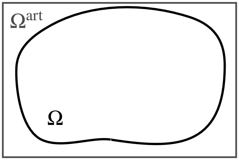
a

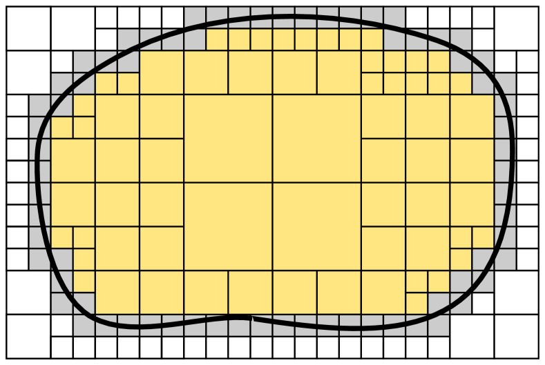
b

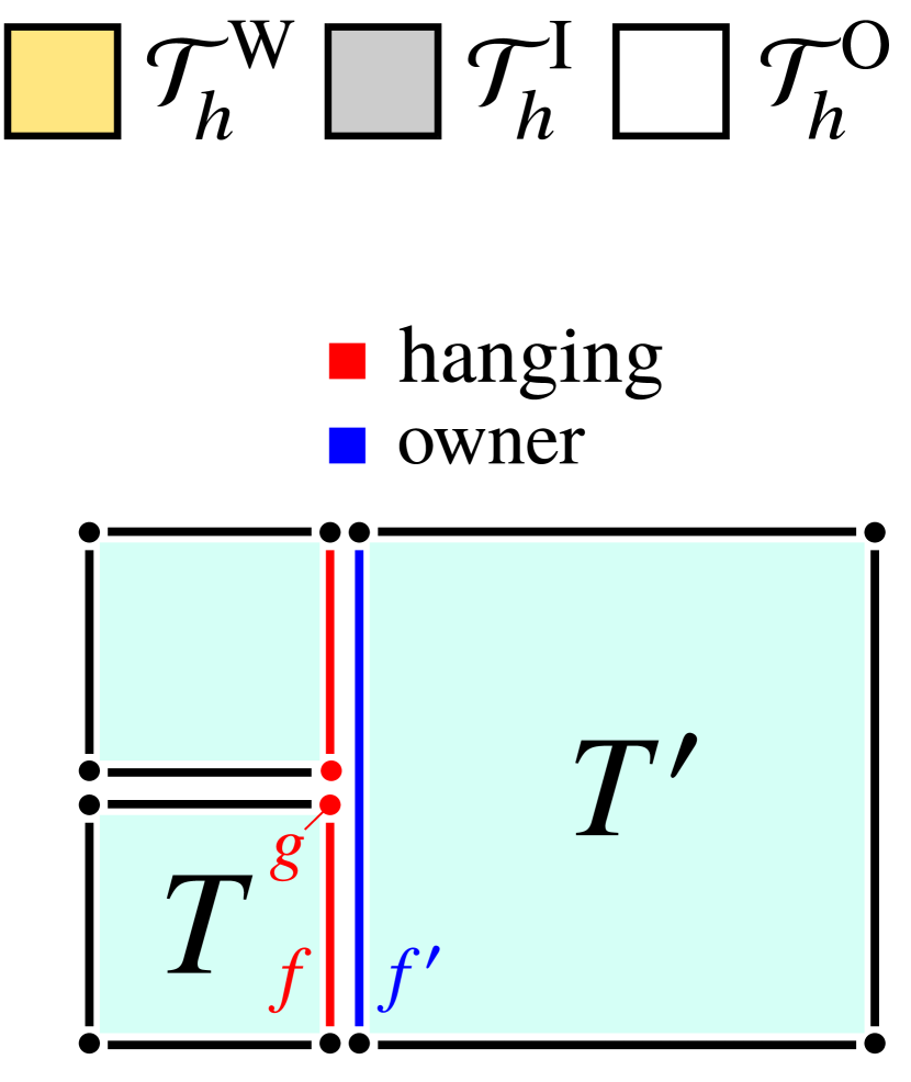
c

Figure 1. We define in (a) a simple artificial domain $\Omega^{\mathrm{art}}$, which includes the physical one $\Omega$. In (b), the background mesh ${\mathcal{T}}_{h}$ meets the 2:1 balance condition. It is partitioned into well-posed ${\mathcal{T}}_{h}^{\mathrm{W}}$, ill-posed ${\mathcal{T}}_{h}^{\mathrm{I}}$ and exterior ${\mathcal{T}}_{h}^{\mathrm{O}}$ cells (we assume $\eta_{0}=1$, i.e. well-posed iff interior and ill-posed iff cut). In (c), we illustrate Assumption 2.1 (ii) with a hanging vertex $g$, a hanging edge $f$ and their owner edge $f^{\prime}$.

As outlined in Section 1, we restrict ourselves to the family of (non-conforming) forest-of-trees meshes. This kind of meshes are derived from recursive application of standard isotropic 1:$2^{d}$ refinement rules on a (possibly unstructured) initial coarse mesh. By construction, they satisfy Assumption 2.1. We choose forest-of-trees, because they are a well-established approach for parallel scalable adaptive mesh generation and partitioning [3]; in particular, we aim to exploit a recent highly-scalable parallel FE framework that supports $h$-adaptivity on forest-of-trees [14].

For FE applications, mesh non-conformity hardens the construction of conforming FE spaces and the subsequent steps in the simulation. For the sake of alleviating this extra complexity, we follow common practice [3, 13] of enforcing the 2:1-balance or 1-irregularity condition, that prescribes, at most, 2:1 size relations between neighbouring cells, see Figure 1b. 2:1 balance ensures that hanging DOF constraints are single-level or direct, i.e. hanging DOFs are not constrained by other hanging DOFs [14, Proposition 3.6]. Furthermore, in a distributed-memory environment, any hanging DOF constraint can be locally applied, as each subdomain holds a single layer of ghost cells [14, Proposition 4.1]. Although the exposition from Sections 2.3 to 2.5 assumes the mesh is a 2:1 balanced forest-of-trees mesh (with isotropic refinements), all concepts introduced there can be generalised to other families of non-conforming meshes, such as anisotropic solvable meshes [31].

We introduce now the immersed boundary setting on top of the artificial domain $\Omega^{\mathrm{art}}$. For the sake of simplicity and without loss of generality, the boundary of the physical domain $\partial\Omega$ is represented by the zero level-set of a known scalar function $\varphi^{\mathrm{ls}}$, namely $\partial\Omega\doteq\{{\boldsymbol{x}}\in\mathbb{R}^{d}:\varphi^{\mathrm{ls}}({\boldsymbol{x}})=0\}$. The problem geometry could be described by other means, e.g. from 3D CAD data, by providing techniques to compute the intersection between cell edges and surfaces. In any case, the following exposition does not depend on the way geometry is handled.

Let now the physical domain be defined as the set of points where the level-set function is negative, namely $\Omega\doteq\{{\boldsymbol{x}}\in\mathbb{R}^{d}:\varphi^{\mathrm{ls}}({\boldsymbol{x}})<0\}$. For any cell $T\in{\mathcal{T}}_{h}$, let us also define the quantity $\eta_{T}\doteq|T\cap\Omega|/|T|$, where $|\cdot|$ denotes the measure (area or volume), and a user-defined parameter $\eta_{0}\in(0,1]$. In order to isolate badly cut cells, we classify cells of ${\mathcal{T}}_{h}$ in terms of $\eta_{T}$ and $\eta_{0}$. A cell $T\in{\mathcal{T}}_{h}$ is: (1) well-posed, if $\eta_{T}\geq\eta_{0}$; (2) ill-posed, if $\eta_{0}>\eta_{T}>0$; or (3) exterior, if $\eta_{T}=0$, i.e. $T\cap\Omega=\emptyset$, see Figure 1b. We remark that, for $\eta_{0}=1$, well-posed cells coincide with interior cells $T\subset\Omega$, whereas ill-posed ones are cut. In the general case, $\eta_{0}\neq 1$, well-posed cells can also be cut cells with a large enough portion inside the physical domain; the distinction between interior and cut cells is no longer relevant. The set of well-posed (resp. ill-posed and exterior) cells is represented with ${\mathcal{T}}_{h}^{\mathrm{W}}$ and its union $\Omega_{\mathrm{W}}=\bigcup_{T\in{\mathcal{T}}_{h}^{\mathrm{W}}}\overline{T}\subset\Omega$ (resp. $({\mathcal{T}}_{h}^{\mathrm{I}},\Omega_{\mathrm{I}})$ and $({\mathcal{T}}_{h}^{\mathrm{O}},\Omega_{\mathrm{O}})$). We also have that $\{{\mathcal{T}}_{h}^{\mathrm{W}},{\mathcal{T}}_{h}^{\mathrm{I}},{\mathcal{T}}_{h}^{\mathrm{O}}\}$ is a partition of ${\mathcal{T}}_{h}$. We let ${\mathcal{T}}_{h}^{\mathrm{act}}\doteq{\mathcal{T}}_{h}^{\mathrm{W}}\cup{\mathcal{T}}_{h}^{\mathrm{I}}$ and $\Omega^{\mathrm{act}}\doteq\Omega_{\mathrm{W}}\cup\Omega_{\mathrm{I}}$ denote the so-called active triangulation and domain.

2.2. Cell aggregation

AgFE spaces are grounded on a cell aggregation map that assigns a well-posed cell to every ill-posed cell. We refer to this map as the root cell map $R:{\mathcal{T}}_{h}\to{\mathcal{T}}_{h}^{\mathrm{W}}$; it takes any cell $T\in{\mathcal{T}}_{h}$ and returns a cell $R(T)\in{\mathcal{T}}_{h}^{\mathrm{W}}$, referred to as the root cell. In order to define this map, we consider a partition of ${\mathcal{T}}_{h}$, denoted by ${\mathcal{T}}_{h}^{\mathrm{ag}}$, into non-overlapping cell aggregates $A_{T}$. Each aggregate $A_{T}$ is a connected set, composed of several ill-posed cells and only one well-posed root cell $T$. Aggregates forming ${\mathcal{T}}_{h}^{\mathrm{ag}}$ are built with a cell aggregation scheme [18] described in Figure 2.

The scheme builds the aggregates incrementally from the (well-posed) root cells, by attaching facet-connected ill-posed cells to them, until all ill-posed cells are aggregated. We recall that facets refer to edges in 2D or faces in 3D. For non-conforming meshes, facet connections comprise those among cells of same or different size. Frequently, an ill-posed cell is facet-connected to several aggregates. Therefore, a criterion is needed to choose among the aggregating candidates. Previous work on uniform meshes [18] adopt a rule that minimises the distance between ill-posed and root cell barycentres. In this way, we keep the characteristic length of the aggregates as small as possible to improve AgFEM’s accuracy . Here, in order to consider the effect of the different cell sizes, it is more adequate to minimise the relative distance between ill-posed and root cell nodes:

Definition 2.2 (Closest root cell criterion).

Given an ill-posed cell $T\in{\mathcal{T}}_{h}$ and the set of aggregating candidates

$$\mathcal{L}(T)=\{T^{\prime}\in{\mathcal{T}}_{h}\,:\,T^{\prime}\text{ is already aggregated and }\exists\text{ a facet }F\in\mathcal{F}_{T}\text{ or }F\in\mathcal{F}_{T^{\prime}}\text{ with }{}\mkern 3.0mu\overline{\mkern-3.0muF}={}\mkern 3.0mu\overline{\mkern-3.0muT}\cap{}\mkern 3.0mu\overline{\mkern-3.0muT^{\prime}},\ F\cap\Omega\neq\emptyset\},$$

that is, $\mathcal{L}$ is the set of aggregated cells connected to $T$ through a conforming or hanging facet $F$. The closest aggregating candidate $T^{*}$ satisfies

$$\tilde{d}(T,T^{*})=\min_{T^{\prime}\in\mathcal{L}(T)}\tilde{d}(T,T^{\prime})$$

with

$$\tilde{d}(T,T^{\prime})\doteq\dfrac{\max_{\gamma\in\mathcal{F}_{R(T^{\prime})}^{0},\delta\in\mathcal{F}_{T}^{0}}\|{\boldsymbol{x}}^{\gamma}-{\boldsymbol{x}}^{\delta}\|_{\infty}}{\max_{\gamma,\gamma^{\prime}\in\mathcal{F}_{R(T^{\prime})}^{0}}\|{\boldsymbol{x}}^{\gamma}-{\boldsymbol{x}}^{\gamma^{\prime}}\|_{\infty}},$$

for any $T^{\prime}\in\mathcal{L}(T)$, where $\mathcal{F}_{T}^{0}$ denotes the set of vertices of $T$, $R(T)$ the root of $T$, ${\boldsymbol{x}}^{\square}$ the coordinates of vertex $\square$ and $\|\cdot\|_{\infty}$ denotes the infinity norm.

When there is more than one closest aggregating candidate $T^{*}$, we simply choose the one whose root cell has higher global cell index. The output of the cell aggregation scheme is the root cell map $R$ and it can be readily applied to arbitrary spatial dimensions. We observe that, by construction of the scheme, maximum aggregate size is bounded above by a constant times the maximum cell size in the mesh [18]. Moreover, in order to assure that aggregates are always connected sets, we assume ${\mathcal{T}}_{h}$ is defined, such that $T\cap\Omega$ is connected, for any $T\in{\mathcal{T}}_{h}$. Connected aggregates are convenient for the numerical analysis in Appendix B, as they allow one to use the Deny-Lions lemma to prove approximability properties.

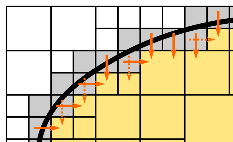
a

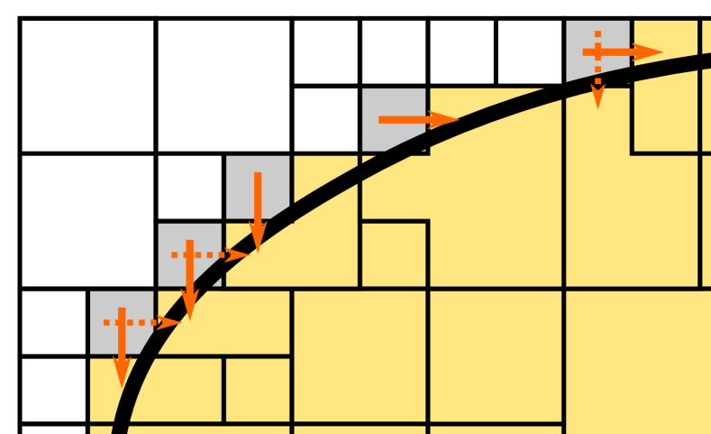
b

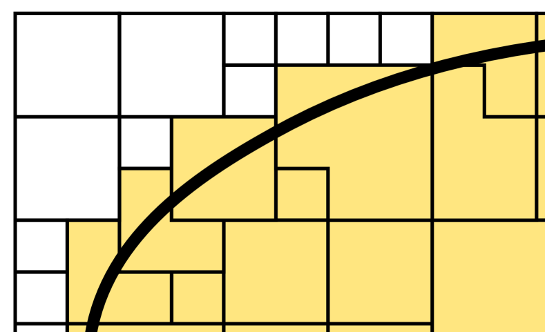
c

Figure 2. Close-up to the top left corner of Figure 1b describing the cell aggregation scheme [18] in three steps. The initial aggregates are well-posed cells; their root cells are assigned to be themselves. Next, we incrementally attach ill-posed cells. An ill-posed cell, when facet-connected to an aggregate, is attached to the closest root cell, in the sense of Definition 2.2. Arrows in (a) and (b) point ill-posed cells to all possible candidates; selected candidates are pointed by continuous arrows, non-selected with discontinuous ones. The black thin lines represent the boundaries of the aggregates. From one step to the next one, some of the lines between adjacent cells are removed. This means that the adjacent cells have been merged into the same aggregate. The procedure leads to ${\mathcal{T}}_{h}^{\mathrm{ag}}$, represented in (c).

2.3. Standard Lagrangian conforming finite element spaces

Our aim now is to present our notation to describe conventional conforming FE spaces on top of tree-based meshes; they are referred to as standard or std, in contrast to the aggregated spaces presented later in Section 2.4. We aim at solving a PDE problem in the physical domain $\Omega$, subject to boundary conditions on $\partial\Omega$. We assume Dirichlet conditions on $\Gamma_{\mathrm{D}}\subset\partial\Omega$. For unfitted meshes, it is not obvious to impose Dirichlet conditions in the approximation space in a strong manner. In consequence, we will assume weak imposition of Dirichlet boundary conditions on $\Gamma_{\mathrm{D}}$.

Our starting point is the typical CG FE space, denoted by ${\mathcal{V}}_{h}^{\mathrm{ncf}}$, in which we enforce continuity across conforming VEFs, i.e. those meeting Assumption 2.1 (i). As usual in FEM, ${\mathcal{V}}_{h}^{\mathrm{ncf}}$ is grounded on defining cell-wise functional spaces $\mathcal{V}(T)$, a canonical basis for a set of local DOFs, a geometrical ownership of the local DOFs by the cell VEFs and a local-to-global map to glue together local DOFs that lie in the same geometrical position. For the sake of simplicity and without loss of generality, we assume the local spaces $\mathcal{V}(T)$ are scalar-valued Lagrangian FEs, of the same order $q$ everywhere. Extension to vector-valued or tensor-valued Lagrangian FEs is straightforward; it suffices to apply the same approach component by component. We denote by $\Sigma$ the set of global DOFs in ${\mathcal{T}}_{h}^{\mathrm{act}}$ associated to ${\mathcal{V}}_{h}^{\mathrm{ncf}}$.

When ${\mathcal{T}}_{h}^{\mathrm{act}}$ is non-conforming, it is clear that ${\mathcal{V}}_{h}^{\mathrm{ncf}}$ yields discontinuous approximations across hanging VEFs. Therefore, the resulting FE space is non-conforming (i.e. it is not a subspace of its infinite-dimensional counterpart) and, thus, not suitable for CG methods. To recover global (trace) continuous FE approximations, values of DOFs lying only on hanging VEFs cannot be arbitrary, they must be linearly constrained. In practice, this means to restrict ${\mathcal{V}}_{h}^{\mathrm{ncf}}$ into a conforming FE subspace ${\mathcal{V}}_{h}^{\mathrm{std}}$.

In order to introduce ${\mathcal{V}}_{h}^{\mathrm{std}}$, let $\Sigma\doteq\{\Sigma^{\mathrm{F}},\Sigma^{\mathrm{H}}\}$ denote a partition into free and hanging DOFs; the latter refers to the subset of global DOFs lying only on hanging VEFs. We let now ${\mathcal{M}}^{{\mathrm{H}}}_{\sigma}$ denote the subset of DOFs constraining $\sigma\in\Sigma^{\mathrm{H}}$, referred to as the set of master DOFs of $\sigma$. Recalling Assumption 2.1 (ii), we observe that, given $\sigma\in\Sigma^{\mathrm{H}}$, lying on a hanging VEF $f$ of a cell $T$, its constraining DOFs are located in the closure of their owner VEF $\overline{f^{\prime}}$ of a coarser cell $T^{\prime}$ [14, Proposition 3.6]. Setup and resolution of hanging DOF constraints for Lagrangian FE spaces is well-established knowledge [11] and, for conciseness, not reproduced here.

Finally, we introduce the standard conforming FE space. Given $v_{h}=\sum_{\sigma\in\Sigma}v^{\sigma}_{h}\phi^{\sigma}\in{\mathcal{V}}_{h}^{\mathrm{ncf}}$, we let

$${\mathcal{V}}_{h}^{\mathrm{std}}\doteq\{v_{h}\in{\mathcal{V}}_{h}^{\mathrm{ncf}}:v^{\sigma}_{h}=\sum_{\sigma^{\prime}\in{\mathcal{M}}^{{\mathrm{H}}}_{\sigma}}C^{\mathrm{H}}_{\sigma\sigma^{\prime}}v_{h}^{\sigma^{\prime}}\ \text{for any}\ \sigma\in\Sigma^{\mathrm{H}}\},$$ (1)

where $C^{\mathrm{H}}_{\sigma\sigma^{\prime}}=\phi^{\sigma^{\prime}}({\boldsymbol{x}}^{\sigma})$ and $\phi^{\sigma^{\prime}}$ is the global shape function of ${\mathcal{V}}_{h}^{\mathrm{ncf}}$ associated with $\sigma^{\prime}$. Note that $C^{\mathrm{H}}_{\sigma\sigma^{\prime}}\neq 0$, by definition of $\sigma\in\Sigma^{\mathrm{H}}$ and ${\mathcal{M}}^{{\mathrm{H}}}_{\sigma}$. We observe that ${\mathcal{V}}_{h}^{\mathrm{std}}\subset{\mathcal{V}}_{h}^{\mathrm{ncf}}$ is conforming, in particular, $v_{h}\in{\mathcal{C}^{0}}(\Omega^{\mathrm{act}})$.

2.4. Aggregated Lagrangian finite element spaces

The space ${\mathcal{V}}_{h}^{\mathrm{std}}$, introduced in Section 2.3, is conforming, but leads to arbitrarily ill-conditioned systems of linear algebraic equations, unless an extra technique is used to remedy it. This is the main motivation to introduce AgFE spaces (see, e.g. [18, 29]). The main idea is to remove from ${\mathcal{V}}_{h}^{\mathrm{std}}$ ill-posed DOFs, associated with small cut cells, by constraining them as a linear combination of DOFs with local support in a well-posed cell. For this purpose, we assign each ill-posed DOF to a well-posed cell, via the root cell map $R$. Following this, we extrapolate the value at the ill-posed DOF, in terms of the DOF values at the root cell. Thus, the problem is posed in terms of well-posed DOFs only, recovering the ill-posed DOFs with a discrete extension operator.

In this section, we derive an AgFE space ${\mathcal{V}}_{h}^{\mathrm{ag}}$ as a subspace of ${\mathcal{V}}_{h}^{\mathrm{std}}$. We focus on laying out the key aspect to combine the new linear constraints, arising from ill-posed DOF removal, with those already restricting ${\mathcal{V}}_{h}^{\mathrm{std}}$, to enforce conformity. For the sake of completeness, we refer to Appendix A for a rigorous description of the extension operator with combined constraints and the proof that ${\mathcal{V}}_{h}^{\mathrm{ag}}$ is well-defined, e.g. it does not have cycling constraint dependencies. Besides, we demonstrate, in Appendix B, (cut-independent) well-posedness and condition number estimates of the linear system arising from this AgFE method on the Poisson problem defined in (3).

In order to construct ${\mathcal{V}}_{h}^{\mathrm{ag}}$, we start by recalling the partition of DOFs associated to ${\mathcal{V}}_{h}^{\mathrm{std}}$ into free DOFs and hanging constrained DOFs. The first and most crucial step is to further distinguish, on top of this partition, among well-posed and ill-posed DOFs. To this end, we must define sets of the form $\Sigma^{{\mathrm{X}},{\mathrm{Y}}}$, where ${\mathrm{X}}\in\{{\mathrm{W}},{\mathrm{I}}\}$ refers to well-posed or ill-posed and ${\mathrm{Y}}\in\{{\mathrm{F}},{\mathrm{H}}\}$ refers to free or hanging. We refer to Figure 3 for an illustration of this classification. The key to combine the constraints is to define well-posed free DOFs $\Sigma^{{\mathrm{W}},{\mathrm{F}}}$ as those with local support in (at least one) a well-posed cell. Specifically, we let $\Sigma^{{\mathrm{W}},{\mathrm{H}}}\subset\Sigma^{\mathrm{H}}$ denote the set of hanging DOFs that are located in ${\mathcal{T}}_{h}^{\mathrm{W}}$, i.e. they are a local DOF of (at least one) well-posed cell. Then, $\Sigma^{{\mathrm{W}},{\mathrm{F}}}\subset\Sigma^{\mathrm{F}}$ is defined as follows.

Definition 2.3.

Given $\sigma\in\Sigma^{\mathrm{F}}$, then $\sigma\in\Sigma^{{\mathrm{W}},{\mathrm{F}}}$ is a well-posed free DOF, if and only if it meets one of the following: (i) $\sigma$ is located in ${\mathcal{T}}_{h}^{\mathrm{W}}$ or (ii) $\sigma$ does not meet condition (i), but $\sigma\in{\mathcal{M}}_{\sigma^{\prime}}^{\mathrm{H}}$ for some $\sigma^{\prime}\in\Sigma^{{\mathrm{W}},{\mathrm{H}}}$, i.e. $\sigma$ is outside ${\mathcal{T}}_{h}^{\mathrm{W}}$, but constrains a well-posed hanging DOF $\sigma^{\prime}$.

$\blacksquare$ $\Omega$   $\blacksquare$ $\Omega^{\mathrm{art}}\setminus\Omega$    $\bullet$ $\Sigma^{{\mathrm{W}},{\mathrm{F}}}$   $\bullet$ $\Sigma^{{\mathrm{W}},{\mathrm{H}}}$   $\boldsymbol{\times}$ $\Sigma^{{\mathrm{I}},{\mathrm{F}}}$   $\boldsymbol{\times}$ $\Sigma^{{\mathrm{I}},{\mathrm{H}}}$

a Correct partition of $\Sigma$ for ${\mathcal{V}}_{h}^{\mathrm{ag}}$. Free DOF $\sigma$ is marked as well-posed, even though it is surrounded by ill-posed cells, because it constrains the well-posed hanging DOF $\sigma^{\prime}$. Hence, it is well-posed due to Definition 2.3 (ii).

b Incorrect partition of $\Sigma$ for ${\mathcal{V}}_{h}^{\mathrm{ag}}$. Free DOF $\sigma$ is marked as ill-posed. If its root cell is pointed by the dashed arrow, then $\sigma^{\prime}$ constrains $\sigma$. In parallel, $\sigma^{\prime}$ is a hanging DOF constrained by $\sigma$. Thus, we have an unsolvable circular constraint dependency.

Figure 3. Classification of $\Sigma$ into $\{\Sigma^{{\mathrm{W}},{\mathrm{F}}},\Sigma^{{\mathrm{W}},{\mathrm{H}}},\Sigma^{{\mathrm{I}},{\mathrm{F}}},\Sigma^{{\mathrm{I}},{\mathrm{H}}}\}$ on a portion of a mesh where $\eta_{0}=1$, i.e. well/ill-posed cell iff interior/cut cell. The key to combine hanging and aggregation DOF constraints is to mark DOFs meeting Definition 2.3 (ii) as well-posed, as in (a). In this way, we circumvent any possible circular constraint dependencies, such as the one described in (b).

This definition eliminates any situation with circular constraint dependencies, as shown in Figure 3b and detailed in Appendix A. Furthermore, it is backed by the numerical analysis in Appendix B. We observe that $\Sigma^{{\mathrm{W}},{\mathrm{F}}}$ includes free DOFs surrounded by ill-posed cells that constrain well-posed hanging DOFs, see Figure 3a. If we let $\Sigma^{{\mathrm{I}},{\mathrm{Y}}}\doteq\Sigma^{{\mathrm{Y}}}\setminus\Sigma^{{\mathrm{W}},{\mathrm{Y}}}$, then it becomes clear that $\{\Sigma^{{\mathrm{W}},{\mathrm{F}}},\Sigma^{{\mathrm{W}},{\mathrm{H}}},\Sigma^{{\mathrm{I}},{\mathrm{F}}},\Sigma^{{\mathrm{I}},{\mathrm{H}}}\}$ is a partition of $\Sigma$. In contrast to free DOFs in $\Sigma^{{\mathrm{W}},{\mathrm{F}}}$, any $\sigma\in\Sigma^{{\mathrm{I}},{\mathrm{F}}}$ is liable to have arbitrarily small local support and, following the AgFEM rationale, must be constrained by DOFs in $\Sigma^{{\mathrm{W}},{\mathrm{F}}}$. It follows that, in the AgFE space, free DOFs are reduced to free well-posed DOFs, i.e. $\Sigma^{{\mathrm{W}},{\mathrm{F}}}$, whereas constrained DOFs are $\Sigma^{\mathrm{C}}\doteq\{\Sigma^{{\mathrm{W}},{\mathrm{H}}},\Sigma^{{\mathrm{I}},{\mathrm{F}}},\Sigma^{{\mathrm{I}},{\mathrm{H}}}\}$. In Appendix A we show that any $\sigma\in\Sigma^{\mathrm{C}}$ can be resolved with direct constraints, i.e. linear constraints of the same form as those in (1), in terms of well-posed free DOFs, only. As a result, the (sequential) aggregated or ag. FE space can be readily defined as

$${\mathcal{V}}_{h}^{\mathrm{ag}}\doteq\{v_{h}\in{\mathcal{V}}_{h}^{\mathrm{ncf}}:v^{\sigma}_{h}=\sum_{\sigma^{\prime}\in{\mathcal{M}}_{\sigma}}C_{\sigma\sigma^{\prime}}v_{h}^{\sigma^{\prime}}\ \text{for any}\ \sigma\in\Sigma^{\mathrm{C}}\},$$ (2)

where ${\mathcal{M}}_{\sigma}$ is the set of DOFs constraining $\sigma\in\Sigma^{\mathrm{C}}$ and $C_{\sigma\sigma^{\prime}}$ is the constraining coefficient for $\sigma^{\prime}\in{\mathcal{M}}_{\sigma}$; we refer to (17) and (18) for their respective full expressions. It is clear that ${\mathcal{V}}_{h}^{\mathrm{ag}}\subset{\mathcal{V}}_{h}^{\mathrm{std}}\subset{\mathcal{V}}_{h}^{\mathrm{ncf}}$. For the sake of brevity, further aspects, such as the definition of the resulting shape basis functions or finite element assembly operations are not covered. In the end, constraints supplementing ${\mathcal{V}}_{h}^{\mathrm{ag}}$ are of multipoint linear type, in the same way as those of ${\mathcal{V}}_{h}^{\mathrm{std}}$; they have been extensively covered in the literature, see, e.g. [27, 12]. With regards to the implementation, we remark that the set up of ${\mathcal{V}}_{h}^{\mathrm{ag}}$ can also potentially reuse data structures and methods devoted to the construction of ${\mathcal{V}}_{h}^{\mathrm{std}}$ or, more generally, any other FE space endowed with linear algebraic constraints.

2.5. Distributed-memory extension

After defining AgFEM in a serial context, we briefly discuss its extension to a domain decomposition (DD) setup for implementation in a distributed-memory computer. We start by setting up the partition of the mesh into subdomains: Let ${\mathcal{S}}$ be a partition of $\Omega^{\mathrm{art}}$ into subdomains obtained by the union of cells in the background mesh ${\mathcal{T}}_{h}$, i.e. for each cell $T\in{\mathcal{T}}_{h}$, there is a subdomain $S\in{\mathcal{S}}$ such that $T\subset S$. We denote by ${\mathcal{T}}_{h}^{{\mathrm{L}}(S)}$ the set of local cells in subdomain $S\in{\mathcal{S}}$; naturally, $\{{\mathcal{T}}_{h}^{{\mathrm{L}}(S)}\}_{S\in{\mathcal{S}}}$ forms a partition of ${\mathcal{T}}_{h}$, see Figure 4. We assume that ${\mathcal{S}}$ is easy to generate. This is a reasonable assumption in our embedded boundary context, where $\Omega^{\mathrm{art}}$ can be easily meshed with e.g. tree-based Cartesian grids, which are amenable to load-balanced partitions grounded on space-filling curves [3].

${\mathcal{T}}_{h}^{{\mathrm{L}}(S_{i})}$   ${\mathcal{T}}_{h}^{{\mathrm{TG}}(S_{i})}$     $S_{1}$     $S_{2}$   $\bullet$ $\Sigma_{\mathrm{L}}^{{\mathrm{W}},{\mathrm{F}}}$   $\bullet$ $\Sigma_{\mathrm{L}}^{{\mathrm{W}},{\mathrm{H}}}$   $\boldsymbol{\times}$ $\Sigma_{\mathrm{L}}^{{\mathrm{I}},{\mathrm{F}}}$   $\boldsymbol{\times}$ $\Sigma_{\mathrm{L}}^{{\mathrm{I}},{\mathrm{H}}}$

a Partial view of ${\mathcal{T}}_{h}^{{\mathrm{L}}(S_{1})}\cup{\mathcal{T}}_{h}^{{\mathrm{TG}}(S_{1})}$.

b Partial view of ${\mathcal{T}}_{h}^{{\mathrm{L}}(S_{2})}\cup{\mathcal{T}}_{h}^{{\mathrm{TG}}(S_{2})}$.

Figure 4. Classification of cells and local DOFs assuming a partition of the mesh portion in Figure 3 into two subdomains. Light-shaded cells are not actually in the scope of $S_{i}$, $i=1,2$. The arrow in (a) points at a free DOF, whose well-posed status can only be known by nearest-neighbour exchange, see Remark 2.4; indeed, it has local support in a well-posed $S_{2}$-cell that is not in ${\mathcal{T}}_{h}^{{\mathrm{L}}(S_{1})}\cup{\mathcal{T}}_{h}^{{\mathrm{TG}}(S_{1})}$.

In a parallel, distributed-memory environment, each subdomain $S$ is mapped to a processor. Thus, each processor holds in memory a portion ${\mathcal{T}}_{h}^{{\mathrm{L}}(S)}$ of the global mesh ${\mathcal{T}}_{h}$. Naturally, local FE integration in $S$ is restricted to cells in ${\mathcal{T}}_{h}^{{\mathrm{L}}(S)}$. However, to correctly perform the parallel FE analysis, the processor-local portion of ${\mathcal{T}}_{h}$ is usually extended with adjacent off-processor cells, a.k.a. ghost cells. Ghost cells are essential to generate the global DOF numbering, in particular, to glue together DOFs in processors that represent the same global DOF. For constrained spaces, they are also needed to locally solve DOF constraints that expand beyond ${\mathcal{T}}_{h}^{{\mathrm{L}}(S)}$. Standard practice in large-scale FE codes is to constrain the ghost cell set to a single layer of ghost cells. Here, we refer to them as the true ghosts, given by ${\mathcal{T}}_{h}^{{\mathrm{TG}}(S)}\doteq\{T\in{\mathcal{T}}_{h}\setminus{\mathcal{T}}_{h}^{{\mathrm{L}}(S)}:\ {}\mkern 1.0mu\overline{\mkern-1.0muT}\cap{}\mkern 1.0mu\overline{\mkern-1.0muS}\neq\emptyset\}$. This layer suffices to glue together global DOFs among processors for non-constrained spaces. However, it is not necessarily enough to meet the requirements of constrained ones.

Our goal in this section is to identify the minimum set of ghost cells that we must attach to ${\mathcal{T}}_{h}^{{\mathrm{L}}(S)}$ in order to define the $S$-subdomain restriction of ${\mathcal{V}}_{h}^{\mathrm{ag}}$ into $S$, which leads to the distributed version of ${\mathcal{V}}_{h}^{\mathrm{ag}}$. Hereafter, all quantities refer to a given subdomain $S$, and we drop the subindex $S$ unless needed for clarity. We assume our initial distributed-memory setting considers processors holding ${\mathcal{T}}_{h}^{\mathrm{L}}\cup{\mathcal{T}}_{h}^{\mathrm{TG}}$ locally. Besides, each processor holds a subdomain restriction of the root cell map $R$, such that it leads to the same aggregates as the ones obtained with the sequential method; see [27] for details on the distributed-memory cell aggregation scheme. We let now $\Sigma_{\mathrm{L}}$ denote the set of ($S$-subdomain) local DOFs, i.e. those located in ${\mathcal{T}}_{h}^{\mathrm{L}}$. As in the sequential version of AgFEM, we have that $\{\Sigma_{\mathrm{L}}^{{\mathrm{W}},{\mathrm{F}}},\Sigma_{\mathrm{L}}^{{\mathrm{W}},{\mathrm{H}}},\Sigma_{\mathrm{L}}^{{\mathrm{I}},{\mathrm{F}}},\Sigma_{\mathrm{L}}^{{\mathrm{I}},{\mathrm{H}}}\}$ forms a partition of $\Sigma_{\mathrm{L}}$, as shown in Figure 4. Hence, $\Sigma_{\mathrm{L}}^{\mathrm{C}}\doteq\{\Sigma_{\mathrm{L}}^{{\mathrm{W}},{\mathrm{H}}},\Sigma_{\mathrm{L}}^{{\mathrm{I}},{\mathrm{F}}},\Sigma_{\mathrm{L}}^{{\mathrm{I}},{\mathrm{H}}}\}$ is the subset of ($S$-subdomain) local constrained DOFs.

For the sake of parallel performance and efficiency, we want to design our parallel algorithms and data structures, concerning the setup of ${\mathcal{V}}_{h}^{\mathrm{ag}}$, in such a way that they maximise local work, while minimising inter-processor communication. In our context, this amounts to ensure that, given $\sigma\in\Sigma_{\mathrm{L}}^{\mathrm{C}}$, we can resolve its full constraint dependency locally, in the scope of the processor. In other words, any constraining DOF $\sigma^{\prime}\in{\mathcal{M}}_{\sigma}$ must be found in the processor-local portion of ${\mathcal{T}}_{h}$. In order to see how we can fulfil this requirement with ${\mathcal{V}}_{h}^{\mathrm{ag}}$, we recover first two particular cases, already addressed in previous literature:

1. ${\mathcal{V}}_{h}^{\mathrm{ag}}$ does not have ill-posed DOFs, i.e. ${\mathcal{V}}_{h}^{\mathrm{ag}}\equiv{\mathcal{V}}_{h}^{\mathrm{std}}$: We recall, from Section 2.3, that constraining DOFs of hanging DOFs are located on their coarser cells around. As all coarser cells around ${\mathcal{T}}_{h}^{\mathrm{L}}$ are in ${\mathcal{T}}_{h}^{\mathrm{L}}\cup{\mathcal{T}}_{h}^{\mathrm{TG}}$, all constraint dependencies of hanging DOFs in ${\mathcal{T}}_{h}^{\mathrm{L}}$ do not expand beyond ${\mathcal{T}}_{h}^{\mathrm{L}}\cup{\mathcal{T}}_{h}^{\mathrm{TG}}$, i.e. all hanging DOF constraints in ${\mathcal{T}}_{h}^{\mathrm{L}}$ can be resolved in ${\mathcal{T}}_{h}^{\mathrm{L}}\cup{\mathcal{T}}_{h}^{\mathrm{TG}}$, see [14, Proposition 4.1].

2. ${\mathcal{V}}_{h}^{\mathrm{ag}}$ does not have hanging DOFs, i.e. ${\mathcal{V}}_{h}^{\mathrm{ag}}$ is defined on a conforming mesh: In general, given $\sigma\in\Sigma_{\mathrm{L}}^{{\mathrm{I}},{\mathrm{F}}}$, the subdomain, where its root cell is located, is different from the current subdomain. In particular, the root cell can be outside ${\mathcal{T}}_{h}^{\mathrm{L}}\cup{\mathcal{T}}_{h}^{\mathrm{TG}}$, as in Figure 5a. This means that the constraint dependency of $\sigma$ propagates away from ${\mathcal{T}}_{h}^{\mathrm{L}}\cup{\mathcal{T}}_{h}^{\mathrm{TG}}$. In order to cancel the constraint associated to $\sigma$, we need to attach the missing root cell to ${\mathcal{T}}_{h}^{\mathrm{L}}\cup{\mathcal{T}}_{h}^{\mathrm{TG}}$ [27]. We let ${\mathcal{T}}_{h}^{\mathrm{RG}}$ denote the set of all missing remote root cells.

  $S_{3}$    $S_{2}$    $S_{1}$  $\bullet$ Free  $\bullet$ Hanging  $\boldsymbol{\times}$ Ill-posed

a Conforming mesh. The value at $\sigma$ is constrained by the nodal values of root cell $T$, which belongs to $S_{3}$. As a result, to resolve the constraint, it is necessary to send to $S_{1}$ data from $T$.

b Non-conforming mesh. In contrast with (a), $T$ touches a coarser cell. Therefore, to fully resolve the constraint it is necessary to send to $S_{1}$ data from $T$ and its coarser neighbour.

Figure 5. An ill-posed DOF $\sigma$ is constrained by a root cell $T$ in $S_{3}$, which is not a neighbour of $S_{1}$.

When both hanging and aggregation DOF constraints are present, the key difference with respect to scenario (2) is that root cells may be in contact with coarser cells. This means that root cells may have hanging DOFs, which are cancelled by DOFs located at their coarser cells around, as pointed out in scenario (1). Therefore, apart from missing root cells, ${\mathcal{T}}_{h}^{\mathrm{RG}}$ must also contain all missing coarser cells around the root cells relevant to $S$, see Figure 5b. Specifically, if $\sigma$ is located in ${\mathcal{T}}_{h}^{\mathrm{L}}\cup{\mathcal{T}}_{h}^{\mathrm{TG}}$, then both the root cell, to which is mapped to, and its coarser cells around should be in the processor-local portion of ${\mathcal{T}}_{h}$. For uniform meshes, algorithms in charge of importing data associated with these missing cells are covered in [27]. They are grounded on the so-called parallel direct and inverse path reconstruction schemes, which only need nearest-neighbour communication patterns. For non-conforming meshes, it suffices to modify them such that they account for non-conforming adjacency in the path reconstruction and also import missing coarser cells around roots into the processor. We stress the fact that this approach does not involve any mesh reconfiguration and repartition, e.g. it keeps the space-filling curve partition, which is essential for performance purposes. It also has little impact on overall parallel performance and scalability and it can be easily implemented in distributed-memory FE codes, as evidenced in Section 3.

In conclusion, if we increment the ghost cell layer with ${\mathcal{T}}_{h}^{\mathrm{RG}}$ as explained above, then we can correctly identify within the processor all constraining DOFs that are located beyond ${\mathcal{T}}_{h}^{\mathrm{L}}$. It follows that we can resolve all hanging and aggregation DOF constraints in ${\mathcal{T}}_{h}^{\mathrm{L}}$ without any extra interprocessor communication, thus achieving our parallel performance target of maximizing local work, while minimising inter-processor communication. Another relevant outcome is that we can accommodate to $\Sigma_{\mathrm{L}}$ the same rationale detailed in Appendix A to solve the mixed constraints; all subsequent steps, to derive expressions for (unified aggregation and hanging) sets of master DOFs and constraining coefficients, follow exactly the sequential AgFEM counterpart, using the corresponding subdomain definitions. It leads to the definition of the distributed version of ${\mathcal{V}}_{h}^{\mathrm{ag}}$ and will not be reproduced here to keep the presentation short.

Remark 2.4.

We observe the following detail: In order to determine whether a free DOF $\sigma\in\Sigma_{\mathrm{L}}$ is well- or ill-posed, i.e. whether $\sigma\in\Sigma_{\mathrm{L}}^{{\mathrm{W}},{\mathrm{F}}}$ or $\sigma\in\Sigma_{\mathrm{L}}^{{\mathrm{I}},{\mathrm{F}}}$, the processor needs to know the set of cells, where $\sigma$ has local support. However, a processor may not know the full set, based solely on local information, i.e. ${\mathcal{T}}_{h}^{\mathrm{L}}\cup{\mathcal{T}}_{h}^{\mathrm{TG}}$. This scenario is illustrated in Figure 4a. Fortunately, to let the processor know the complete set of cells, it suffices to combine the local information with a single nearest-neighbour communication. This result is backed by [14, Proposition 4.3], where an analogous issue is described, when trying to recover all the processors where $\sigma$ has local support, instead of its well- or ill-posed cell status.

3. Numerical experiments

Our purpose in this section is to assess numerically the behaviour of $h$-AgFEM. We start with a description of the model problem in Section 3.1. We consider a Poisson equation with non-homogeneous Dirichlet boundary conditions and a Nitsche-type variational form. We introduce next the experimental benchmarks in Section 3.2, composed of several manufactured problems defined in a set of complex geometries. After this, we jump into the numerical experiments themselves. We describe and discuss the results of two sets of experiments, namely convergence tests in Section 3.3 and weak-scaling tests in Section 3.4.

3.1. Model problem

Numerical examples consider the Poisson equation with non-homogeneous Dirichlet boundary conditions. After scaling with the diffusion term, the equation reads: find $u\in H^{1}(\Omega)$ such that

$$-\Delta u=f,\quad\text{in}\ \Omega,\qquad u=g,\quad\text{on}\ \Gamma_{\mathrm{D}}\doteq\partial\Omega,$$ (3)

where $f\in H^{-1}(\Omega)$ is the source term and $g\in H^{1/2}(\partial\Omega)$ is the prescribed value on the Dirichlet boundary. In the numerical tests, we study both ${\mathcal{V}}_{h}^{\mathrm{std}}$ and ${\mathcal{V}}_{h}^{\mathrm{ag}}$, see Sections 2.3 and 2.4, as possible choices of ${\mathcal{V}}_{h}^{\rm x}$. As stated in Section 2.3, we consider weak imposition of boundary conditions, since unfitted methods do not easily accommodate prescribed values in a strong sense. As usual in the embedded boundary community, we resort to Nitsche’s method to circumvent this problem [18, 17, 16]. We observe that this approach provides a consistent numerical scheme with optimal convergence rates (even for high-order FEs). According to this, we approximate (3) with the variational formulation: find $u_{h}\in{\mathcal{V}}_{h}^{\rm x}$ such that $\mathrm{a}(u_{h},v_{h})=\mathrm{b}(v_{h})$ for all $v_{h}\in{\mathcal{V}}_{h}^{\rm x}$, with

$$\begin{array}[]{l}\displaystyle\mathrm{a}(u_{h},v_{h})\doteq\int_{\Omega}\nabla u_{h}\cdot\nabla v_{h}\mathrm{\ d}\Omega+\int_{\partial\Omega}\left(\tau u_{h}v_{h}-u_{h}\left(\boldsymbol{n}\cdot\nabla v_{h}\right)-v_{h}\left(\boldsymbol{n}\cdot\nabla u_{h}\right)\right)\mathrm{\ d}{\Gamma},\quad\text{and}\\ \displaystyle\mathrm{b}(v_{h})\doteq\int_{\Omega}v_{h}f\mathrm{\ d}\Omega+\int_{\partial\Omega}\left(\tau v_{h}g-\left(\boldsymbol{n}\cdot\nabla v_{h}\right)g\right)\mathrm{\ d}\Gamma,\end{array}$$ (4)

with $\boldsymbol{n}$ being the outward unit normal on $\partial\Omega$. We note that forms $\mathrm{a}(\cdot,\cdot)$ and $\mathrm{b}(\cdot)$ include the usual terms, resulting from the integration by parts of (3), plus additional terms associated with the weak imposition of Dirichlet boundary conditions with Nitsche’s method. For further details, we refer to Appendix B.2, where we prove well-posedness of Problem (4) considering ${\mathcal{V}}_{h}^{\mathrm{ag}}$ as the discretisation space.

Coefficient $\tau>0$ denotes a mesh-dependent parameter that has to be large enough to ensure coercivity of $\mathrm{a}(\cdot,\cdot)$. It is prescribed with the same rationale given in [27, Section 4.2]. For ${\mathcal{V}}_{h}^{\mathrm{ag}}$, we have that $\tau={\beta^{\mathrm{ag}}}{h_{T}^{-1}}$ for all $T\in{\mathcal{T}}_{h}^{\mathrm{I}}$, where $h_{T}$ is the cell characteristic size and $\beta^{\mathrm{ag}}$ is a user-defined constant parameter. Numerical experiments take $\beta^{\mathrm{ag}}=25.0$; this value is enough for having a well-posed problem in all cases considered in Section 3.3. When using ${\mathcal{V}}_{h}^{\mathrm{std}}$, the value in a generic ill-posed cell takes the form

$$\tau=\beta^{\mathrm{std}}\lambda_{T}^{\max},\ \text{for all}\ T\in{\mathcal{T}}_{h}^{\mathrm{I}},$$ (5)

where $\beta^{\mathrm{std}}=2.0$ and $\lambda_{T}^{\max}$ is the maximum eigenvalue of the generalised eigenvalue problem: find $\mu_{T}\in{\mathcal{V}}_{h}^{\mathrm{std}}|_{T}$ and $\lambda_{T}\in\mathbb{R}$ such that

$$\int_{T\cap\Omega}\nabla\mu_{T}\cdot\nabla\xi_{T}\mathrm{\ d}\Omega=\lambda_{T}\int_{T\cap\partial\Omega}(\nabla\mu_{T}\cdot\boldsymbol{n})(\nabla\xi_{T}\cdot\boldsymbol{n})\mathrm{\ d}\Gamma,\enskip\text{for all}\ \xi_{T}\in{\mathcal{V}}_{h}^{\mathrm{std}}|_{T},\enskip\text{for all}\ T\in{\mathcal{T}}_{h}^{\mathrm{I}}.$$

We notice that $\tau$ computed as in (5) can be arbitrarily large, as the measure of the cut $\Omega\cap T$, $T\in{\mathcal{T}}_{h}^{\mathrm{I}}$, tends to zero. This means that, in contrast with ${\mathcal{V}}_{h}^{\mathrm{ag}}$, strongly ill-conditioned systems of linear equations may arise with ${\mathcal{V}}_{h}^{\mathrm{std}}$, depending on the position of the cut.

3.2. Experimental setup

The model problem is defined on five different 2D and 3D non-trivial domains shown in Figure 6: (a) a planar “pacman" shape, (b) a popcorn flake with a wedge removed, (c) a hollow block, (d) a 3-by-3 array of (c) and (e) a spiral. These geometries appear often in the literature to study robustness and performance of unfitted FE methods (see, e.g. [16, 18]). The artificial domain $\Omega^{\mathrm{art}}$, on top of which the mesh is generated, is the cuboid $\left[-1,1\right]^{d}$, $d=2,3$, for cases (a-c), $\left[0,1\right]^{3}$ for case (d) and $\left[-1,1\right]^{2}\times\left[0,2\right]$ for case (e).

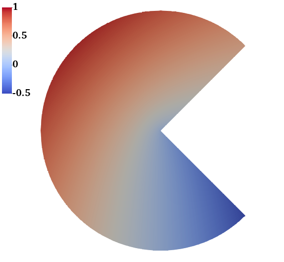
a Pacman

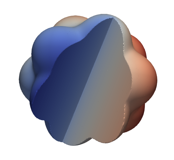
b Popcorn

c Hollow block

d H. b. array

e Spiral

Figure 6. Geometries and numerical solution to the problems studied in the examples. (a-b) consider the Fichera corner problem in (6), whereas (c-e) the multiple “shock" in (7).

As illustrated in Figure 6, for geometries (a-b), the source term and boundary conditions of the Poisson equation are defined, such that the PDE has the exact solution

$$u(r,\theta)=r^{\alpha}\sin\alpha\theta,\ r=\sqrt{x^{2}+y^{2}},\ \theta=\arctan y/x,\ \alpha=2/3,$$ (6)

$$(x,y)\in\Omega\subset\mathbb{R}^{2},\ z=0\text{ in 2D},\qquad(x,y,z)\in\Omega\subset\mathbb{R}^{3}\text{ in 3D}.$$

The same applies to (c-e), but seeking a different exact solution given by

$$u(r) =\sum_{i=1,3}\arctan\tau^{i}(r-r_{0}^{i}),$$ (7)

$$r=||{\boldsymbol{x}}-{\boldsymbol{x}}_{0}^{i}||_{2},\ {\boldsymbol{x}} =(x,y,z)\in\Omega\subset\mathbb{R}^{3},$$

where $\|\cdot\|_{2}$ denotes the Euclidean norm and

$$\begin{array}[]{lll}\tau^{1}=60,&(x_{0}^{1},y_{0}^{1},z_{0}^{1})=(-1,-1,1),&r_{0}^{1}=2.5,\\ \tau^{2}=80,&(x_{0}^{2},y_{0}^{2},z_{0}^{2})=(1,1,-1),&r_{0}^{2}=1.75,\text{ and }\\ \tau^{3}=120,&(x_{0}^{3},y_{0}^{3},z_{0}^{3})=(0.5,-3,-3),&r_{0}^{3}=4.5.\end{array}$$

Problems (6) and (7) correspond to adapted versions of two classical hp-FEM benchmarks, namely, the Fichera corner and “shock" problems (see, e.g. [32]). Derivatives of solution $u$ in (6) are singular at the $r=0$ axis; in particular, $u\in H^{1+\frac{2}{3}}(\Omega)$. Recalling a priori error estimates, it is well known that the rate of convergence of the standard FE method with uniform $h$-refinements, when applied to this case, is bounded by regularity only. Specifically, the energy-norm error satisfies $\|u-u_{h}\|_{a}\leq Ch^{-2/3}\|u\|_{H^{1+\frac{2}{3}}(\Omega)}$. However, by combining a posteriori error estimation and $h$-adaptive refinements, optimal rates of convergence can be restored [32]. On the other hand, problem (7) is characterised by three intersecting shocks. The solution to the problem is smooth, but it sharply varies in the neighbourhood of the shocks. In this case, $h$-adaptive standard FEM does not affect rates of convergence, but potentially yields meshes that minimise the number of cells required to achieve a given discretisation error.

The variety of shapes and benchmarks considered here aims to show (i) the capability of $h$-AgFEM of retaining the same benefits $h$-adaptivity brings, when combined with standard FEM, while being able (ii) to deal with complex and diverse 2D and 3D domains in a robust manner and (iii) to yield remarkable parallel efficiency with state-of-the-art out-of-the-box scalable iterative linear solvers for symmetric positive definite matrices. In order to do this, we confront numerical results obtained with ${\mathcal{V}}_{h}^{\mathrm{ag}}$ against those of ${\mathcal{V}}_{h}^{\mathrm{std}}$. In the plots, the two spaces are labelled as aggregated (or ag.) and standard (or std.). All examples run on background Cartesian grids, with standard isotropic 1:4 (2D) and 1:8 (3D) refinement rules; they are commonly referred to as quad- or octrees in 2D or 3D, resp. Apart from that, continuous FE spaces composed of first order Lagrangian finite elements are employed.

In the numerical experiments, we perform convergence tests using three different remeshing strategies (uniform refinements, Li and Bettess (LB) and Oñate and Bugeda (OB) [33, 34]) in a parallel, distributed-memory environment. We also assess robustness to cut location and assess sensitivity to the well-posedness threshold $\eta_{0}$. Finally, we perform a weak scalability analysis for some selected ag. cases; Table 1 summarises the main parameters and computational strategies used in the numerical examples.

We carry out the numerical experiments at the Marenostrum-IV (MN-IV) supercomputer, hosted by the Barcelona Supercomputing Centre. Concerning the software, an MPI-parallel implementation of the $h$-AgFEM method is available at FEMPAR [30]. FEMPAR is linked against p4est v2.2 [3], as the octree Cartesian grid manipulation engine, and PETSc v3.11.1 [28] distributed-memory linear algebra data structures and solvers. To show that ${\mathcal{V}}_{h}^{\mathrm{ag}}$ leads to systems, that are amenable to well established scalable linear solvers for standard FE analysis on body-fitted meshes, we resort to the broad suite of linear solvers available in the PETSc library [28]. In particular, we use a conjugate gradient (CG) method, preconditioned by a smoothed-aggregation AMG scheme called GAMG. The preconditioner is set up in favour of reducing, as much as possible, the deviation from its default configuration, as in [27]. We do this in order to show that AgFEM blends well with common AMG solvers, whereas std. unfitted FEM does not. Both solver and preconditioner are readily available through the Krylov Methods KSP module of PETSc. In order to advance convergence tests down to low global energy-norm error values, without being polluted by the linear solver accuracy, convergence of GAMG is declared when $\|\mathbf{r}\|_{2}/\|\mathbf{b}\|_{2}<10^{-9}$ within the first $500$ iterations, where $\mathbf{r}\doteq\mathbf{b}-\mathbf{A}\mathbf{x}^{\rm cg}$ is the unpreconditioned residual.

Description	Considered methods/values
Model problem	Poisson equation (Nitsche’s formulation)
Problem geometry	2D: Pacman shape; 3D: Popcorn flake,
	Hollow block, Hollow block array and spiral
AMR benchmark	Fichera corner and multiple-shock problem [32]
Remeshing strategy	Uniform, Li and Bettess [33], and Oñate and Bugeda [34]
Experimental computer environment	Parallel (distributed-memory)
Mesh topology	Single quad- or octree
Parallel mesh generation and partitioning tool	p4est library [3]
Well-posed cut cell criterion	$\eta_{0}=0.25$
FE spaces	Aggregated ${\mathcal{V}}_{h}^{\mathrm{ag}}$ and standard ${\mathcal{V}}_{h}^{\mathrm{std}}$
Cell type	Hexahedral cells
Interpolation	Piece-wise bi/trilinear shape functions
Linear solver	Preconditioned conjugate gradients
Parallel preconditioner	Smoothed-aggregation GAMG
GAMG stopping criterion	$\|\mathbf{r}\|_{2}/\|\mathbf{b}\|_{2}<10^{-9}$
Coef. in Nitsche’s penalty term for ${\mathcal{V}}_{h}^{\mathrm{ag}}$	$\beta=25.0$

Table 1. Summary of the main parameters and computational strategies used in the numerical examples.

3.3. Convergence tests

Convergence tests in relative energy-norm error are carried out with three different mesh refinement strategies. The first one is uniform $h$-refinements, in pursuance of both exposing the behaviour of AgFEM, in absence of hanging node constraints, and the limited regularity of the Fichera corner problem. The remaining two are error-driven; they are distinguished by different optimality criteria on the elemental error indicator $\gamma_{T}$, for any $T\in{\mathcal{T}}_{h}$. It is not in the scope of this work to design a posteriori error estimation techniques for AgFEM, although there are some works with other unfitted FE methods that explore this question [10]. Hence, since the target problems have known analytical solution, $\gamma_{T}$ is taken as the energy norm of the local true error $e=u-u_{h}$, that is,

$$\gamma_{T}=\|e\|_{{\left.a\right|_{T\cap\Omega}}}=\|u-u_{h}\|_{{\left.a\right|_{T\cap\Omega}}},\quad T\in{\mathcal{T}}_{h}.$$

Error-driven mesh adaptation seeks an optimal mesh with an iterative procedure. In the examples below, optimality is declared when the global absolute discretisation error, measured in energy norm, $\|e\|_{a}$ is below a prescribed quantity $\gamma$, i.e.

$$\|e\|_{a}\leq\gamma,\quad\gamma>0.$$ (8)

(8) is referred to as the acceptability criterion.

The process starts with an initial guess of the optimal mesh. After finding the approximate solution and the exact cell-wise error distribution, a new mesh is defined with a remeshing strategy. This step consists in comparing each $\gamma_{T}$ to a given threshold, commonly known as the optimality criterion, which is later defined. Depending on the result of the comparison, a different remeshing flag is assigned to the cell. If $\gamma_{T}$ is above the threshold, $T$ is marked for refinement. Otherwise, $T$ is left unmarked or, optionally, marked for coarsening, when $\gamma_{T}$ falls well below the threshold. Following this, the mesh is transformed, according to the cell-wise remeshing flags, and partitioned. Next, a new FE space is created, by distributing DOFs on top of the new mesh and computing the nonconforming DOF constraints and, if using ${\mathcal{V}}_{h}^{\mathrm{ag}}$, also the ill-posed DOF constraints. After FE integration and assembly, the resulting linear system is solved and the cell-wise error distribution is updated. If the current mesh complies with the acceptability criterion of (8), the process is stopped, otherwise it goes back to the application of the optimality criterion.

As mentioned before, two different optimality criteria (thresholds for refinement) are studiedThe first one, the LB [35, 33] criterion, establishes that the error distribution in an optimal mesh (denoted with *) is uniform, that is

$$\|e^{*}\|_{T^{*}\cap\Omega}=\frac{\gamma}{\sqrt{M^{*}}},\quad T^{*}=1,\ldots,M^{*},$$ (9)

where $M^{*}$ is the number of cells in the optimal mesh. At each mesh adaptation step, this quantity is estimated as

$$M^{*}=\gamma^{-d/m}\left(\sum_{T=1}^{M}\|e\|_{T}^{d/(m+d/2)}\right)^{(m+d/2)/m},$$ (10)

with $d$ the space dimension, $m$ the degree of the interpolation (in second-order elliptic problems) and $M$ the number of cells of the current iteration. On the other hand, the OB [34] criterion considers that the distribution of error density in an optimal mesh is uniform, that is

$$\|e^{*}\|_{T^{*}\cap\Omega}=\frac{\gamma\Omega_{T^{*}\cap\Omega}^{1/2}}{\Omega^{1/2}},\quad T^{*}=1,\ldots,M^{*},$$ (11)

where $\Omega$ is the measure of the domain and $\Omega_{T^{*}\cap\Omega}$ is the measure of $T^{*}\cap\Omega$. While the former criterion has been proved [35] to provide standard body-fitted FE meshes satisfying (8) with the least number of elements, the latter scales the threshold in terms of the size of the (ill-posed) cell. One of the goals of the following experiments is to see how both strategies perform in the context of unfitted FEs. Note that, with respect to standard body-fitted FEM, both remeshing strategies are almost applied verbatim to an unfitted FE setting; the only difference being that the local quantities in cut cells are computed in the interior part only, in the same way as for the local integration of the weak form stated in (4).

Convergence tests with uniform $h$-refinements follow the usual procedure, whereas error-driven tests are controlled with a finite sequence of decreasing error objectives $\gamma_{i}$, $i>1$. For each $i>1$, the iterative procedure described above is carried out to find the mesh that complies with the acceptability criterion of (8) with $\gamma=\gamma_{i}$. If subscript $\gamma_{i}$ refers to the quantities obtained at the last mesh iteration, at the end of the procedure we can extract the pair

$$\left(\frac{\|e\|_{a,\gamma_{i}}}{\|u\|_{a,\gamma_{i}}},N_{\mathrm{dofs}}^{\gamma_{i}}\right),$$

that is, a point of the convergence test curve. Figure 7 depicts some meshes found with this iterative procedure, using the LB acceptability criterion.

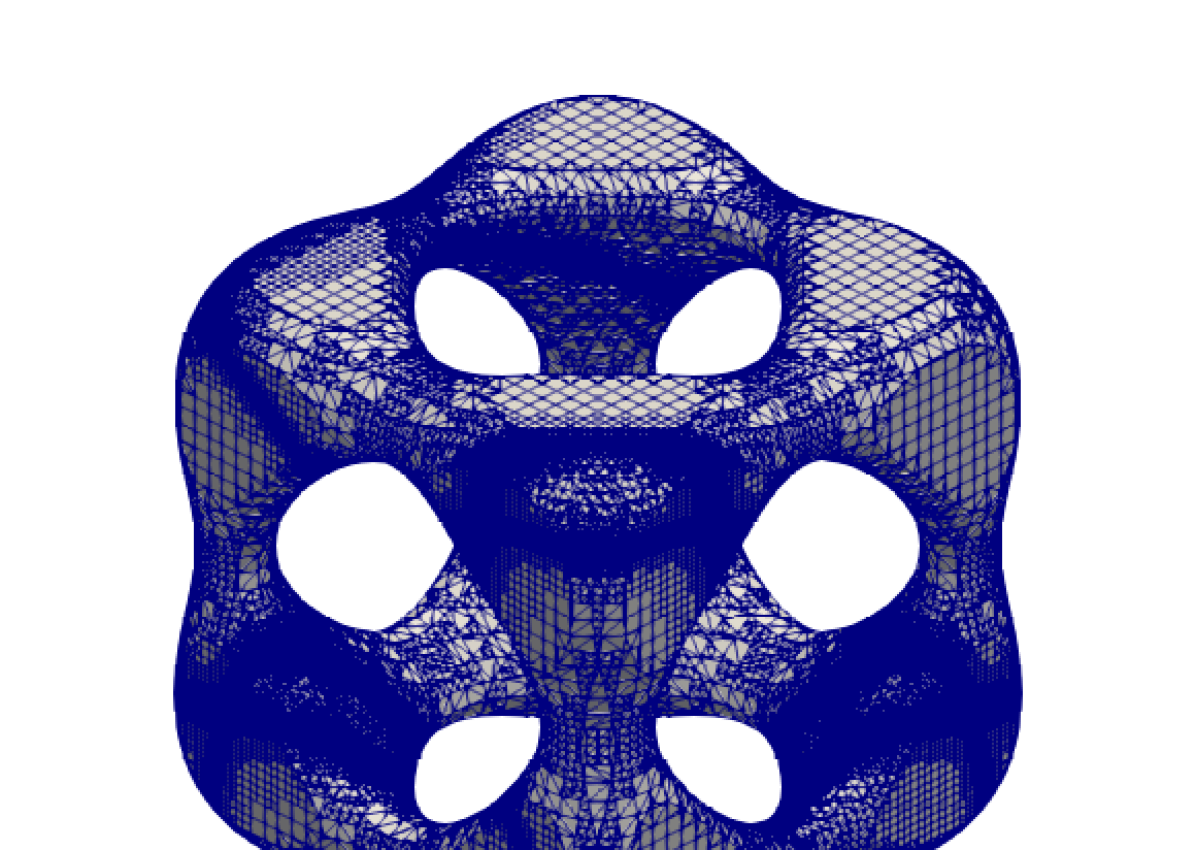
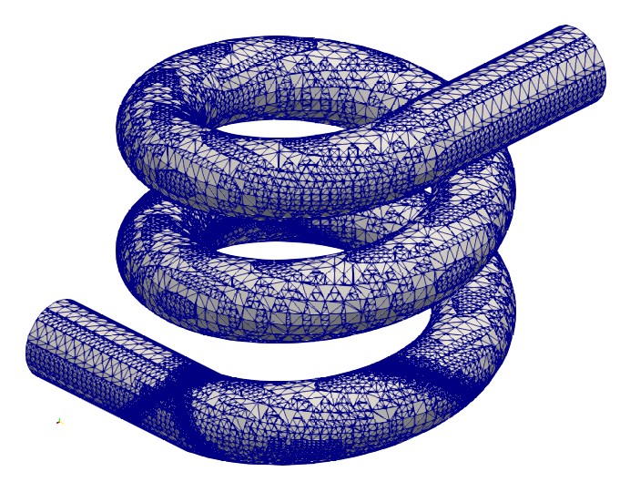
Figure 7. Pacman-Fichera, hollow-shock and spiral-shock examples: optimal meshes obtained with the LB criterion for the convergence test.

We carry out all convergence tests for a fixed number of threads (MPI tasks). We employ six MN-IV high-memory nodes and map each core to a different MPI task. Therefore, the experiments are launched in $6\cdot 48=288$ processors. The partition of the mesh considers $288$ subdomains and is defined to seek an equal distribution of the number of cells among processors (p4est default setting). The well-posedness threshold for aggregation $\eta_{0}$ (see Section 2.2) is prescribed to $0.25$ in what follows.

Let us now start the discussion of the numerical results obtained with convergence tests. As shown in Figure 8 $h$-AgFEM behaviour consistently mirrors the one of std. $h$-FEM. This includes that (1) $h$-AgFEM always produces more optimal meshes, in terms of the error, than its non-adaptive version; and (2) optimal convergence rates are retained, even for the $h$-AgFEM Fichera problems, where convergence in the non-adaptive version is limited by regularity.

Although the std. method is slightly more accurate than its ag. counterpart for the Fichera problems with uniform refinements, the usual behaviour is that they are very similar in terms of accuracy. Another outcome observed is that the LB criterion is clearly more cost-efficient, in terms of mesh size, than the OB one for both std. and ag. variants. This is also reported in [36] with std. $h$-FEM.

However, as expected, the linear solver does not manage to generate a solution in most of std. FE cases. Either the preconditioner cannot be generated or it is not positive definite (thus, incompatible with the conjugate gradient method). Both issues are directly related to the severe ill-conditioning of matrices obtained with the std. method, as extensively reported in previous works [18, 27]. On the other hand, when using the ag. method, GAMG is fully robust and converges towards the solution at the $10^{-9}$ tolerance.

a Pacman-Fichera

b Popcorn-Fichera

c Block-Shock

d Array-Shock

e Spiral-Shock

Figure 8. Convergence tests in parallel environment for 288 tasks.

Despite poor robustness of the solver with the std. method, available results in Figure 9 are enough to clearly identify higher growth rates in number of iterations for std. matrices, than for ag. ones. This exposes that, among the two methods, only $h$-AgFEM is potentially scalable, as the number of iterations mildly grows with the size of the problem; even for $h$-AgFEM points in Figure 9 with the largest number of DOFs, convergence is declared in almost twenty iterations. We have verified that, in this context, the solver achieves single-digit reduction of the residual norm in 2-3 iterations, at most. Textbook multigrid efficiency is attained when the solver uses a modest number of point smoothing steps and convergence nearly advances at one digit in reduction of the residual norm per iteration [28]. We have checked the former is satisfied, by inspecting PETSc log data, whereas the latter is broadly fulfilled in AgFEM experiments. Therefore, GAMG on $h$-AgFEM matrices is not only robust, but also efficient.

a Pacman-Fichera

b Popcorn-Fichera

c Block-Shock

d Array-Shock

e Spiral-Shock

Figure 9. GAMG solver iterations in parallel environment for 288 number of tasks.

A final experiment with convergence tests looks at the sensitivity of AgFEM to the well-posedness threshold $\eta_{0}$. As it is shown in Figure 10, low values of $\eta_{0}$ may not bypass the small cut-cell problem and hinder GAMG solvability, as shown in the 3D parallel examples. Conversely, high values of $\eta_{0}$ do not affect robustness, but increase solver iterations and reduce (local) accuracy. This is most likely an effect of excessive well-posed-to-ill-posed DOF extrapolation. As a result, optimal $\eta_{0}$ values may be found in the middle of the $[0,1]$ range. This means that, while enforcing a minimum amount of aggregation is required to guarantee robustness, superfluous aggregation deteriorates solver efficiency. This effect is particularly prominent in $h$-adaptivity; setting $\eta_{0}=1$ on uniform meshes leads to decent results, as demonstrated in a previous work [27].

a Pacman-F. conv. in parallel

b Popcorn-F. conv. in parallel

c Block-s. conv. in parallel

d Pacman-F. GAMG iterations

e Popcorn-F. GAMG iterations

f Block-s. GAMG iterations

Figure 10. $h$-AgFEM sensitivity to $\eta_{0}$ with the LB criterion. Recall that $\eta_{0}=0.25$ is the reference value in previous experiments (see Figures 8-9).

3.4. Weak scaling

The starting point of weak scaling tests is the parallel convergence test setup of the previous section. As explained, a single convergence test case results in a set of pairs

$$\left\{\left(\frac{\|e\|_{a,\gamma_{i}}}{\|u\|_{a,\gamma_{i}}},N_{\mathrm{dofs}}^{\gamma_{i}}\right)\right\}_{\gamma_{i}>1},$$

associated with a finite sequence of decreasing target error values $\gamma_{i}$, $i>1$. Each test corresponds to an individual curve, e.g. the LB-ag curve for the Pacman-Fichera test case in Figure 8a. Other quantities can be extracted from the test, e.g. the size of the global triangulation $N_{\mathrm{cells}}^{\gamma_{i}}$. In Section 3.3, each pair was obtained for a fixed number of processors $P=288$. Naturally, as $N_{\mathrm{cells}}^{\gamma_{i}}$ increases with $i$, so does the size of the local portion of the triangulation $n_{\mathrm{cells}}^{\gamma_{i}}$, owned by each processor.

Given $\left\{N_{\mathrm{cells}}^{\gamma_{i}}\right\}_{i>1}$ associated with a convergence test, a weak scaling one can be derived by adjusting the number of processors $P^{i}$ for each $\gamma_{i}$, such that $n_{\mathrm{cells}}^{\gamma_{i}}$ remains approximately constant for all $i>1$. This can be achieved, by e.g. prescribing

$$P^{i}=P^{1}\left\lfloor\frac{N_{\mathrm{cells}}^{\gamma_{i}}}{N_{\mathrm{cells}}^{\gamma_{1}}}\right\rfloor,\ i>1,$$

where $P^{1}$ is a fixed initial number of processors and $\lfloor\cdot\rfloor$ is the floor function; given a real number $x$, $\lfloor x\rfloor$ is the greatest integer less than or equal to $x$. From here, the weak scaling test consists merely in repeating the convergence test, taking $P^{i}$ processors for each $\gamma_{i}$. In this way, by keeping the local size of the mesh $n_{\mathrm{cells}}^{\gamma_{i}}$ constant, we can straightforwardly study how $h$-AgFEM scales with global size of the problem. Table 2 gathers the sequences $\left\{P^{i}\right\}_{i>1}$ obtained following this procedure for the two test cases that will be studied in this section, namely, the Popcorn-Fichera and Hollow-Shock problems for the AgFEM method with the LB remeshing criterion and $\eta_{0}=0.25$.

Popcorn-Fichera LB-ag with $\eta_{0}=0.25$ and $n_{\mathrm{cells}}\approx 15.5k$
$P$	2	8	19	52	132	349	883
$N_{\mathrm{cells}}$	31k	130k	301k	800k	2,025k	5,354k	13,553k
Hollow-shock LB-ag with $\eta_{0}=0.25$ and $n_{\mathrm{cells}}\approx 21.0k$
$P$	6	17	29	107	194	790	1,484
$N_{\mathrm{cells}}$	126k	369k	612k	2,261k	4,083k	16,662k	31,221k

Table 2. Number of subdomains and total cells in the background mesh for the cases considered in the weak scaling tests of Figure 11. For each case, local mesh size, given by $n_{\mathrm{cells}}$, remains quasi-constant with the number of subdomains $P$.

In weak scaling tests, we monitor wall clock times spent in the main phases of (i) the AgFEM method and (ii) the linear solver. We additionally get (iii) the number of GAMG solver iterations. As finding the optimal mesh for each $\gamma_{i}$, $i>1$ is an iterative AMR process, we only report these quantities for the optimal mesh (last iteration). In the FE simulation loop, the starting control point is right after generating and partitioning the optimal mesh. From here, and following the order of the simulation pipeline, we report the time consumed in relevant AgFEM-related phases

1. parallel cell aggregation, i.e. generation of the distributed-memory root cell map $R$ (Section 2.2),

2. import data from missing remote root (and their coarse neighbour) cells, i.e. import ${\mathcal{T}}_{h}^{{\mathrm{RG}}}$ (Section 2.5),

3. setup of the distributed ${\mathcal{V}}_{h}^{\mathrm{std}}$ space (Section 2.3), accounting for hanging DOF constraints,

4. setup of the distributed ${\mathcal{V}}_{h}^{\mathrm{ag}}$ space on top of ${\mathcal{V}}_{h}^{\mathrm{std}}$ (Sections 2.4 and 2.5), with mixed hanging and aggregation DOF constraints.

This is followed (and completed) by gathering the time spent in the linear solver setup and run stages, as well as the number of solver iterations needed to find the approximate solution to the problem on the optimal mesh. The convergence criterion is the same as the one of the previous section, i.e. $\|\mathbf{r}\|_{2}/\|\mathbf{b}\|_{2}<10^{-9}$.

To allocate the MPI tasks in the MN-IV supercomputer, we resort to the default task placement policy of Intel MPI (v2018.4.057) with partially filled nodes. For each point of the test, the number of nodes $N^{i}$ is selected as $N^{i}=\left\lceil P^{i}/48\right\rceil$, where $\lceil\cdot\rceil$ is the ceiling function; given a real number $x$, $\lceil x\rceil$ is the smallest integer more than or equal to $x$. If $P^{i}$ is not multiple of 48, the placement policy fully populates the first $N-1$ nodes with 48 MPI tasks per node; the remaining $P^{i}-48(N-1)$ MPI tasks are mapped to the last node.

Figure 11 gathers all the quantities surveyed in weak scaling tests. All main phases of the $h$-AgFEM method exhibit remarkable scalability (Figures 11a and 11b). The results are also qualitatively similar for both geometries. Concerning solver performance in Figures 11c-11f, although times and iterations do not scale as well as $h$-AgFEM-specific phases, results are still sound. Different system matrix conditioning could explain the slight differences between the two problems in solver performance. In any case, growth rate is mild, compared to growth of problem size. For instance, in the Hollow-shock example, total solver wall clock time (setup plus run) scales from 0.55 to 2.34 s, while the problem size scales from 126,232 to 16,619,828 cells. This means the total solver time increases by a factor of $4.3x$, whereas the problem size by a factor of $131.7x$. On the other hand, solver degradation is likely not fully attributed to $h$-AgFEM; see, e.g. the results in [27], showing that GAMG loses parallel efficiency even when dealing with body-fitted meshes.

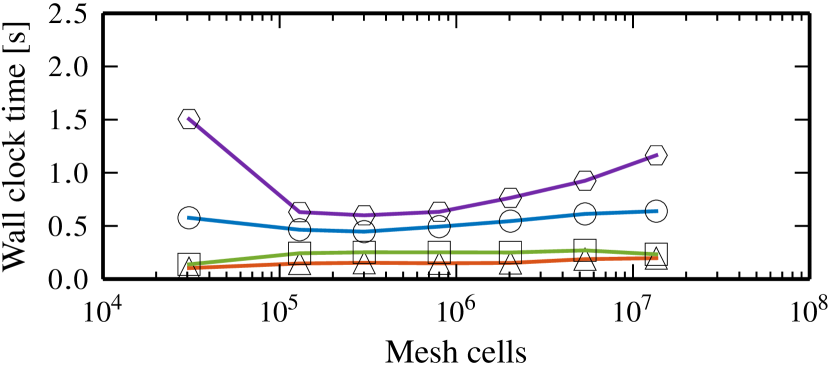
a Popcorn-Fichera LB $\eta_{0}=0.25$

b Hollow-shock LB $\eta_{0}=0.25$

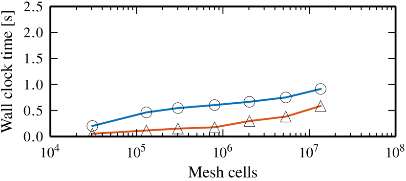
c Popcorn-Fichera LB $\eta_{0}=0.25$

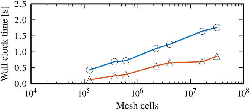
d Hollow-shock LB $\eta_{0}=0.25$

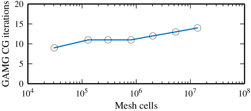
e Popcorn-Fichera LB $\eta_{0}=0.25$

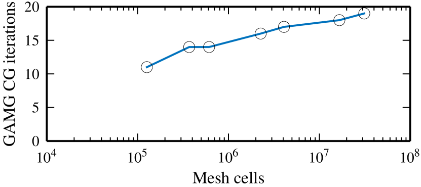
f Hollow-shock LB $\eta_{0}=0.25$

Figure 11. AgFEM weak scaling tests up to 1,484 MPI tasks, as specified in Table 2.

4. Conclusions

In this work, we have introduced the aggregated finite element method on parallel adaptive tree-based meshes, referred to as $h$-AgFEM. The main difficulty is to establish how to combine hanging DOF constraints, arising from mesh non-conformity, with aggregation ones, which are needed to get rid of the small cut cell problem, in the definition of the discrete extension operator from well-posed to ill-posed DOFs. We have followed a two-level strategy, grounded on building the aggregated FE space on top of an existing conforming FE space.

As main contributions of the paper, we have shown that (a) our approach allows one to define a unified AgFE space accounting for both type of constraints, without circular constraint dependencies; the key point is to mark as ill-posed DOFs those without local support in a well-posed cell. We have also described how, (b) by carefully extending the layer of ghost cells, a distributed-memory version of $h$-AgFEM can be easily incorporated into existing large-scale FE codes. With numerical experimentation on the Poisson problem, we have studied the behaviour of $h$-AgFEM. It (c) enjoys the same benefits of standard $h$-FEM on body-fitted meshes. In particular, it restores optimal rates of convergence, implied by order of approximation alone, and it is amenable to standard mesh optimality criteria. Likewise, it also (d) inherits good properties from AgFEM on uniform meshes, above all robustness with respect to cut location. We have also demonstrated (e) good parallel performance of a distributed-memory implementation of $h$-AgFEM; the main outcome is that it can efficiently exploit well-known AMG preconditioners available in, e.g. PETSc. Finally, we have (f) carried out a complete numerical analysis that supports the design of the method and the numerical results.

We have successfully managed to bridge unfitted methods and parallel non-conforming tree-based meshes for the first time. $h$-AgFEM has the potential to grow and tackle large-scale multi-phase and multi-physics FE applications on arbitrarily complex geometries, aided by functional and geometrical error-driven mesh adaptation. As future work, it also remains to extend $h$-AgFEM to high-order FE approximations and, more generally, $hp$-adaptivity.

Appendix A Derivation of the AgFE space ${\mathcal{V}}_{h}^{\mathrm{ag}}$

In this appendix, our goal is to show that any constrained DOF $\sigma\in\Sigma^{\mathrm{C}}$ of the AgFE space ${\mathcal{V}}_{h}^{\mathrm{ag}}$ given in  (2), can be resolved with direct constraints. This means that it is composed by linear constraints of the same form as those in (1), i.e. in terms of well-posed free DOFs, only. For this purpose, we go over each subset of $\Sigma^{\mathrm{C}}$ and characterise the subsets of $\Sigma^{{\mathrm{W}},{\mathrm{F}}}$ constraining them, as well as the coefficients of the linear constraints. We also argue that the resulting constraint dependency graph, drawn in Figure 12, has no cyclic constraint dependencies. The discussion leads to the definition of an aggregated FE space ${\mathcal{V}}_{h}^{\mathrm{ag}}$ that is a subspace of ${\mathcal{V}}_{h}^{\mathrm{std}}$ with the same structure, i.e. restricted with linear constraints.

Figure 12. Constraint dependency graph of the AgFE space ${\mathcal{V}}_{h}^{\mathrm{ag}}$. The set of global DOFs $\Sigma$ is partitioned into $\{\Sigma^{{\mathrm{W}},{\mathrm{F}}},\Sigma^{{\mathrm{W}},{\mathrm{H}}},\Sigma^{{\mathrm{I}},{\mathrm{F}}},\Sigma^{{\mathrm{I}},{\mathrm{H}}}\}$. Subsets $\Sigma^{{\mathrm{W}},{\mathrm{H}}}$, $\Sigma^{{\mathrm{I}},{\mathrm{F}}}$ and $\Sigma^{{\mathrm{I}},{\mathrm{H}}}$ are all constrained by $\Sigma^{{\mathrm{W}},{\mathrm{F}}}$ with a dependency graph represented by dashed blue edges marked with a ${\mathrm{C}}$. Dashed blue edges link a constrained subset with the subsets where its masters belong to. We observe that the graph has no cycles.

According to this, given $\sigma\in\Sigma^{\mathrm{C}}$,

1. if $\sigma\in\Sigma^{{\mathrm{W}},{\mathrm{H}}}$, then ${\mathcal{M}}^{\mathrm{H}}_{\sigma}$ is formed by DOFs located in VEFs of coarser neighbour cells around $\sigma$, see Section 2.3. As ${\mathcal{T}}_{h}$ meets the 2:1 balance condition, constraining DOFs of hanging DOFs are free DOFs [14, Proposition 4.1], i.e.

   $$\sigma\in\Sigma^{\mathrm{H}}\Rightarrow{\mathcal{M}}^{\mathrm{H}}_{\sigma}\subset\Sigma^{\mathrm{F}}.$$ (12)

   Recalling Definition 2.3 (ii), it follows that master DOFs of $\sigma$ are necessarily contained in the set of well-posed free DOFs, i.e.

   $$\sigma\in\Sigma^{{\mathrm{W}},{\mathrm{H}}}\Rightarrow{\mathcal{M}}^{\mathrm{H}}_{\sigma}\subset\Sigma^{{\mathrm{W}},{\mathrm{F}}}.$$ (13)

   Therefore, linear constraints of $\sigma\in\Sigma^{{\mathrm{W}},{\mathrm{H}}}$ remain unchanged in the new AgFE space.

2. If $\sigma\in\Sigma^{{\mathrm{I}},{\mathrm{F}}}$, then we assume that we have composed the root cell map $R:{\mathcal{T}}_{h}^{\mathrm{act}}\to{\mathcal{T}}_{h}^{\mathrm{W}}$, introduced in Section 2.2, with a map between ill-posed free DOFs $\Sigma^{{\mathrm{I}},{\mathrm{F}}}$ and ill-posed cells ${\mathcal{T}}_{h}^{\mathrm{I}}$. In other words, we assign first each ill-posed free DOF to one of its surrounding ill-posed cells. The chosen cell is then mapped onto a well-posed cell via $R$. Thus, the outcome of this composition is a map $K:\Sigma^{{\mathrm{I}},{\mathrm{F}}}\to{\mathcal{T}}_{h}^{\mathrm{W}}$, that assigns an ill-posed free DOF to a well-posed cell; see formal definitions in, e.g. [27, 18]. Given $\sigma\in\Sigma^{{\mathrm{I}},{\mathrm{F}}}$, let us denote by ${\mathcal{M}}^{{\mathrm{A}}{\mathrm{A}}}_{\sigma}$ the subset of DOFs $\tilde{\sigma}$ located in $K(\sigma)$, such that $\phi^{\tilde{\sigma}}({\boldsymbol{x}}^{\sigma})\neq 0$. We refer to ${\mathcal{M}}^{{\mathrm{A}}{\mathrm{A}}}_{\sigma}$ as the set of “direct” AgFEM master DOFs of $\sigma\in\Sigma^{{\mathrm{I}},{\mathrm{F}}}$. As usual in AgFE methods, given $v_{h}\in{\mathcal{V}}_{h}^{\mathrm{std}}$ and $\sigma\in\Sigma^{{\mathrm{I}},{\mathrm{F}}}$, we enforce the constraint

   $$v^{\sigma}_{h}=\sum_{\tilde{\sigma}\in{\mathcal{M}}^{{\mathrm{A}}{\mathrm{A}}}_{\sigma}}C^{{\mathrm{A}}{\mathrm{A}}}_{\sigma\tilde{\sigma}}v_{h}^{\tilde{\sigma}},\quad\text{with}\ C^{{\mathrm{A}}{\mathrm{A}}}_{\sigma\tilde{\sigma}}\doteq\phi^{\tilde{\sigma}}({\boldsymbol{x}}^{\sigma}),$$ (14)

   that is, we linearly extrapolate the nodal value of an ill-posed DOF with the values at the local DOFs of its root cell. In general, ${\mathcal{M}}^{{\mathrm{A}}{\mathrm{A}}}_{\sigma}$ is composed of both free and hanging DOFs, i.e. some DOFs in the root cell can be hanging; the latter are not master DOFs, in the strict sense, and we need to remove them, i.e. rewrite (14) in terms of well-posed free DOFs, only. For that purpose, we introduce the partition ${\mathcal{M}}^{{\mathrm{A}}{\mathrm{A}}}_{\sigma}=\{{\mathcal{M}}^{{\mathrm{A}}{\mathrm{F}}}_{\sigma},{\mathcal{M}}^{{\mathrm{A}}{\mathrm{H}}}_{\sigma}\}$, with ${\mathcal{M}}^{{\mathrm{A}}{\mathrm{F}}}_{\sigma}\doteq{\mathcal{M}}^{{\mathrm{A}}{\mathrm{A}}}_{\sigma}\cap\Sigma^{{\mathrm{F}}}$, ${\mathcal{M}}^{{\mathrm{A}}{\mathrm{H}}}_{\sigma}\doteq{\mathcal{M}}^{{\mathrm{A}}{\mathrm{A}}}_{\sigma}\cap\Sigma^{{\mathrm{H}}}$. Since the image of $K$ is in ${\mathcal{T}}_{h}^{\mathrm{W}}$, it is clear that ${\mathcal{M}}^{{\mathrm{A}}{\mathrm{F}}}_{\sigma}\subset\Sigma^{{\mathrm{W}},{\mathrm{F}}}$ and ${\mathcal{M}}^{{\mathrm{A}}{\mathrm{H}}}_{\sigma}\subset\Sigma^{{\mathrm{W}},{\mathrm{H}}}$. We also have that

   $$\sigma\in\Sigma^{{\mathrm{I}},{\mathrm{F}}}\Rightarrow{\mathcal{M}}^{{\mathrm{A}}{\mathrm{A}}}_{\sigma}\subset\Sigma^{{\mathrm{W}},{\mathrm{F}}}\cup\Sigma^{{\mathrm{W}},{\mathrm{H}}}.$$ (15)

   Recalling the first case, i.e. $\sigma\in\Sigma^{{\mathrm{W}},{\mathrm{H}}}$, the set of DOFs that are masters of ${\mathcal{M}}^{{\mathrm{A}}{\mathrm{H}}}_{\sigma}$ is given by $\bigcup_{\sigma^{\prime}\in{\mathcal{M}}^{{\mathrm{A}}{\mathrm{H}}}_{\sigma}}{\mathcal{M}}^{\mathrm{H}}_{\sigma^{\prime}}$ and, by (13), it is included in $\Sigma^{{\mathrm{W}},{\mathrm{F}}}$. If the previous property didn’t hold, then $\Sigma^{{\mathrm{I}},{\mathrm{F}}}\cap\left(\bigcup_{\sigma^{\prime}\in{\mathcal{M}}^{{\mathrm{A}}{\mathrm{H}}}_{\sigma}}{\mathcal{M}}^{\mathrm{H}}_{\sigma^{\prime}}\right)\neq\emptyset$ and it could be possible that $\sigma\in\bigcup_{\sigma^{\prime}\in{\mathcal{M}}^{{\mathrm{A}}{\mathrm{H}}}_{\sigma}}{\mathcal{M}}^{\mathrm{H}}_{\sigma^{\prime}}$, i.e. $\sigma$ could (circularly) constrain itself, as in the situation depicted in Figure 3b.

   Hence, the “true” set of master DOFs of $\sigma\in\Sigma^{{\mathrm{I}},{\mathrm{F}}}$ is ${\mathcal{M}}^{\mathrm{A}}_{\sigma}\doteq{\mathcal{M}}^{{\mathrm{A}}{\mathrm{F}}}_{\sigma}\cup\left(\bigcup_{\sigma^{\prime}\in{\mathcal{M}}^{{\mathrm{A}}{\mathrm{H}}}_{\sigma}}{\mathcal{M}}^{\mathrm{H}}_{\sigma^{\prime}}\right)$; note that the two set members of ${\mathcal{M}}^{\mathrm{A}}_{\sigma}$ are not necessarily disjoint, but ${\mathcal{M}}^{\mathrm{A}}_{\sigma}\subset\Sigma^{{\mathrm{W}},{\mathrm{F}}}$. Besides, recalling that hanging DOFs are constrained by free DOFs on top of VEFs of coarser neighbour cells, ${\mathcal{M}}^{\mathrm{A}}_{\sigma}$ are composed of DOFs located in root cells and (neighbouring) coarser cells around them.

   After cancelling hanging DOFs, we can derive an analogous expression to (14), in terms of well-posed free DOFs only. The value of the AgFEM constraint, for $\sigma\in\Sigma^{{\mathrm{I}},{\mathrm{F}}}$ and $\tilde{\sigma}\in{\mathcal{M}}^{\mathrm{A}}_{\sigma}$, is

   $$C^{\mathrm{A}}_{\sigma\tilde{\sigma}}\doteq\left\{\begin{array}[]{ll}C^{{\mathrm{A}}{\mathrm{A}}}_{\sigma\tilde{\sigma}}&\text{if}\ \tilde{\sigma}\in{\mathcal{M}}^{{\mathrm{A}}{\mathrm{F}}}_{\sigma},\ \text{only}\\ C^{{\mathrm{A}}{\mathrm{A}}}_{\sigma\tilde{\sigma}}+\sum_{\left(\sigma^{\prime}\in{\mathcal{M}}^{{\mathrm{A}}{\mathrm{H}}}_{\sigma}\ \text{s.t.}\ \tilde{\sigma}\in{\mathcal{M}}^{\mathrm{H}}_{\sigma^{\prime}}\right)}C^{{\mathrm{A}}{\mathrm{A}}}_{\sigma\sigma^{\prime}}C^{\mathrm{H}}_{\sigma^{\prime}\tilde{\sigma}}&\text{if}\ \tilde{\sigma}\in{\mathcal{M}}^{{\mathrm{A}}{\mathrm{F}}}_{\sigma}\cap\left(\bigcup_{\sigma^{\prime}\in{\mathcal{M}}^{{\mathrm{A}}{\mathrm{H}}}_{\sigma}}{\mathcal{M}}^{\mathrm{H}}_{\sigma^{\prime}}\right)\\ \sum_{\left(\sigma^{\prime}\in{\mathcal{M}}^{{\mathrm{A}}{\mathrm{H}}}_{\sigma}\ \text{s.t.}\ \tilde{\sigma}\in{\mathcal{M}}^{\mathrm{H}}_{\sigma^{\prime}}\right)}C^{{\mathrm{A}}{\mathrm{A}}}_{\sigma\sigma^{\prime}}C^{\mathrm{H}}_{\sigma^{\prime}\tilde{\sigma}}&\text{if}\ \tilde{\sigma}\in\bigcup_{\sigma^{\prime}\in{\mathcal{M}}^{{\mathrm{A}}{\mathrm{H}}}_{\sigma}}{\mathcal{M}}^{\mathrm{H}}_{\sigma^{\prime}},\ \text{only}.\end{array}\right.$$ (16)

   We refer to Figure 13 for an illustration of the three types of $\tilde{\sigma}\in{\mathcal{M}}_{\sigma}^{\mathrm{A}}$ in (16).

   Figure 13. Close-up of Figure 3a. Assuming that the top right ill-posed DOF is mapped to the well-posed cell pointed by the dashed arrow, we mark with letters and classify all DOFs $\tilde{\sigma}\in{\mathcal{M}}_{\sigma}^{\mathrm{A}}$, as they are distinguished in (16). In this sense, (a) shows $\tilde{\sigma}\in{\mathcal{M}}_{\sigma}^{{\mathrm{A}}{\mathrm{F}}}$, only; (b) shows $\tilde{\sigma}\in{\mathcal{M}}_{\sigma}^{{\mathrm{A}}{\mathrm{F}}}\cap\left(\bigcup_{\sigma^{\prime}\in{\mathcal{M}}^{{\mathrm{A}}{\mathrm{H}}}_{\sigma}}{\mathcal{M}}^{\mathrm{H}}_{\sigma^{\prime}}\right)$; (c) shows $\tilde{\sigma}\in\bigcup_{\sigma^{\prime}\in{\mathcal{M}}^{{\mathrm{A}}{\mathrm{H}}}_{\sigma}}{\mathcal{M}}^{\mathrm{H}}_{\sigma^{\prime}}$, only. We observe that DOFs (c) are only in neighbouring coarser cells.

3. If $\sigma\in\Sigma^{{\mathrm{I}},{\mathrm{H}}}$, then $\sigma$ cannot be constrained as in the previous case, i.e. hanging DOF constraints have to be imposed first, to preserve conformity. According to this, $\sigma$ can be constrained by either well-posed or ill-posed free DOFs, i.e. ${\mathcal{M}}^{\mathrm{H}}_{\sigma}\subset\Sigma^{{\mathrm{W}},{\mathrm{F}}}\cup\Sigma^{{\mathrm{I}},{\mathrm{F}}}$; this is an immediate consequence of (12). If we consider now a partition of ${\mathcal{M}}^{\mathrm{H}}_{\sigma}$ into well-posed and ill-posed master DOFs and use case $\sigma\in\Sigma^{{\mathrm{I}},{\mathrm{F}}}$ to remove ill-posed master DOFs, we deduce that

   $${\mathcal{M}}^{\mathrm{H}}_{\sigma}=\left({\mathcal{M}}^{\mathrm{H}}_{\sigma}\cap\Sigma^{{\mathrm{W}},{\mathrm{F}}}\right)\cup\left({\mathcal{M}}^{\mathrm{H}}_{\sigma}\cap\Sigma^{{\mathrm{I}},{\mathrm{F}}}\right)=\left({\mathcal{M}}^{\mathrm{H}}_{\sigma}\cap\Sigma^{{\mathrm{W}},{\mathrm{F}}}\right)\cup\left(\bigcup_{\sigma^{\prime}\in{\mathcal{M}}^{\mathrm{H}}_{\sigma}\cap\Sigma^{{\mathrm{I}},{\mathrm{F}}}}{\mathcal{M}}^{\mathrm{A}}_{\sigma^{\prime}}\right)\subset\Sigma^{{\mathrm{W}},{\mathrm{F}}},$$

   i.e. we can compute the constraints in terms of well-posed free DOFs only; again the two sets in the right-hand side are not necessarily disjoint. After cancelling the AgFEM constraints of $\sigma^{\prime}\in{\mathcal{M}}^{\mathrm{H}}_{\sigma}\cap\Sigma^{{\mathrm{I}},{\mathrm{F}}}$, the constraint coefficient for $\sigma\in\Sigma^{{\mathrm{I}},{\mathrm{H}}}$ and $\sigma^{\prime}\in{\mathcal{M}}^{\mathrm{H}}_{\sigma}$ becomes

   $$C^{{\mathrm{H}}{\mathrm{A}}}_{\sigma\sigma^{\prime}}\doteq\left\{\begin{array}[]{ll}{\mathrm{C}}^{\mathrm{H}}_{\sigma\sigma^{\prime}}&\text{if}\ \sigma^{\prime}\in\left({\mathcal{M}}^{\mathrm{H}}_{\sigma}\cap\Sigma^{{\mathrm{W}},{\mathrm{F}}}\right),\ \text{only}\\ {\mathrm{C}}^{\mathrm{H}}_{\sigma\sigma^{\prime}}+\sum_{\left(\tilde{\sigma}\in{\mathcal{M}}^{\mathrm{A}}_{\sigma}\ \text{s.t.}\ \sigma^{\prime}\in{\mathcal{M}}^{\mathrm{H}}_{\tilde{\sigma}}\right)}C^{\mathrm{A}}_{\sigma\tilde{\sigma}}C^{\mathrm{H}}_{\tilde{\sigma}\sigma^{\prime}}&\text{if}\ \left({\mathcal{M}}^{\mathrm{H}}_{\sigma}\cap\Sigma^{{\mathrm{W}},{\mathrm{F}}}\right)\cap\left(\bigcup_{\sigma^{\prime}\in{\mathcal{M}}^{\mathrm{H}}_{\sigma}\cap\Sigma^{{\mathrm{I}},{\mathrm{F}}}}{\mathcal{M}}^{\mathrm{A}}_{\sigma^{\prime}}\right)\\ \sum_{\left(\tilde{\sigma}\in{\mathcal{M}}^{\mathrm{A}}_{\sigma}\ \text{s.t.}\ \sigma^{\prime}\in{\mathcal{M}}^{\mathrm{H}}_{\tilde{\sigma}}\right)}C^{\mathrm{A}}_{\sigma\tilde{\sigma}}C^{\mathrm{H}}_{\tilde{\sigma}\sigma^{\prime}}&\text{otherwise}.\end{array}\right.$$

The last step to derive the AgFE space is to gather the previous cases, combining hanging and aggregation DOF constraints, into a unified form equivalent to (14). Given $\sigma\in\Sigma^{\mathrm{C}}$, the set of master DOFs is

$${\mathcal{M}}_{\sigma}\doteq\left\{\begin{array}[]{ll}{\mathcal{M}}^{\mathrm{H}}_{\sigma}&\text{if}\ \sigma\in\Sigma^{{\mathrm{W}},{\mathrm{H}}}\\ {\mathcal{M}}^{\mathrm{A}}_{\sigma}&\text{if}\ \sigma\in\Sigma^{{\mathrm{I}},{\mathrm{F}}}\\ \left({\mathcal{M}}^{\mathrm{H}}_{\sigma}\cap\Sigma^{{\mathrm{W}},{\mathrm{F}}}\right)\cup\left(\bigcup_{\sigma^{\prime}\in{\mathcal{M}}^{\mathrm{H}}_{\sigma}\cap\Sigma^{{\mathrm{I}},{\mathrm{F}}}}{\mathcal{M}}^{\mathrm{A}}_{\sigma^{\prime}}\right)&\text{if}\ \sigma\in\Sigma^{{\mathrm{I}},{\mathrm{H}}}.\end{array}\right.$$ (17)

By definition, ${\mathcal{M}}_{\sigma}\subset\Sigma^{{\mathrm{W}},{\mathrm{F}}}$, for all $\sigma\in\Sigma^{\mathrm{C}}$, i.e. all constraints can be solved by free well-posed DOFs and, thus, there are no cyclic constraint dependencies; see also the constraint dependency graph represented in Figure 12. On the other hand, the constraint coefficient for $\sigma\in\Sigma^{\mathrm{C}}$ and $\sigma^{\prime}\in{\mathcal{M}}_{\sigma}$ is

$$C_{\sigma\sigma^{\prime}}\doteq\left\{\begin{array}[]{ll}{\mathrm{C}}^{\mathrm{H}}_{\sigma\sigma^{\prime}}&\text{if}\ \sigma\in\Sigma^{{\mathrm{W}},{\mathrm{H}}}\\ {\mathrm{C}}^{\mathrm{A}}_{\sigma\sigma^{\prime}}&\text{if}\ \sigma\in\Sigma^{{\mathrm{I}},{\mathrm{F}}}\\ {\mathrm{C}}^{{\mathrm{H}}{\mathrm{A}}}_{\sigma\sigma^{\prime}}&\text{if}\ \sigma\in\Sigma^{{\mathrm{I}},{\mathrm{H}}}.\end{array}\right.$$ (18)

With these notations, the (sequential) aggregated or ag. FE space ${\mathcal{V}}_{h}^{\mathrm{ag}}$ obeys to the form stated in  (2).

Appendix B Numerical analysis

In this appendix, we prove that both the condition number of (a) the mass matrix associated to the AgFE space defined in (2) and (b) the linear system arising from (4) are bounded. The bounds do not depend on the cut location (but they do depend on the well-posedness threshold $\eta_{0}$). We use the notation $A\lesssim B$ (resp. $A\gtrsim B$) to represent $A\leq CB$ (resp. $A\geq CB$) for a positive constant $C>0$ independent of the interface-mesh intersection or the mesh cells sizes.

B.1. Mass matrix condition number

In order to bound the condition number of the mass matrix, we seek to show the equivalence, for functions in ${\mathcal{V}}_{h}^{\mathrm{ag}}$, between the $L^{2}(\Omega)$-norm and the Euclidean norm of well-posed free DOFs. We devote the next paragraphs to introduce necessary definitions and preliminary results. Given $u_{h}\in{\mathcal{V}}_{h}^{\mathrm{ag}}$, let us denote the nodal vector of well-posed free DOFs by ${\underline{\mathbf{u}}}$. For a given $T\in{\mathcal{T}}_{h}$ and VEF $f$, the cell- or VEF-wise coordinate vector is represented with ${\underline{\mathbf{u}}}_{T}$ or ${\underline{\mathbf{u}}}_{f}$ and its characteristic sizes by $h_{T}$ or $h_{f}$. First, we rely on the maximum and minimum eigenvalues of the local mass matrix in the physical cell $T$ or any of its VEFs $f\in\mathcal{F}_{T}$:

$$\lambda_{\min}h_{X}^{d_{X}}\|{\underline{\mathbf{u}}}_{X}\|_{2}^{2}\leq\|u_{h}\|_{L^{2}(X)}^{2}\leq\lambda_{\max}h_{X}^{d_{X}}\|{\underline{\mathbf{u}}}_{X}\|_{2}^{2},\quad\text{for}\ u_{h}\in\mathcal{V}(T),$$ (19)

with $X=T$ or $X=f\in\mathcal{F}_{T}$ and $\|\cdot\|_{2}$ denoting the Euclidean norm. The values of $\lambda_{\min}$, $\lambda_{\max}>0$ only depend on the order of the FE space and can be computed for different orders on $n$-cubes or $n$-simplices [37]. By combining (19) for $T$ and one of its VEFs, we deduce the bound

$$\|u_{h}\|_{L^{2}(T)}^{2}\gtrsim h_{f}^{d-d_{f}}\|u_{h}\|_{L^{2}(f)}^{2}>0,\quad\text{for}\ u_{h}\in\mathcal{V}(T),\ f\in\mathcal{F}_{T}.$$ (20)

We observe that (20) can be applied to any $T\in{\mathcal{T}}_{h}^{\mathrm{W}}$ and corresponding VEFs, because we are integrating on the whole objects. If we consider integration on the cut portion of the cell $\Omega\cap T$, (19) also holds, up to a positive constant that depends on the well-posedness threshold $\eta_{0}$. This is a consequence of the following result.

Lemma B.1.

Given a well-posed cell $T\in{\mathcal{T}}_{h}^{\mathrm{W}}$ and $u_{h}\in\mathcal{V}(T)$, there exists $C(\eta_{0})>0$, dependent on the well-posedness threshold $\eta_{0}$, such that $\|u_{h}\|_{L^{2}(\Omega\cap T)}^{2}\geq C(\eta_{0})\|u_{h}\|_{L^{2}(T)}^{2}$.

Proof.

Since we consider a well-posedness threshold $0<\eta_{0}\leq 1$, any cell $T\in{\mathcal{T}}_{h}^{\mathrm{W}}$ can be either (i) (full) interior or (ii) cut. For case (i), the bound trivially holds. For case (ii), given any polynomial defined in the cell, in particular, any shape function, we must have that $\int_{\Omega\cap T}{p(x)}^{2}\geq C(\eta_{0})\int_{T}{p(x)}^{2}>0$, for a bounded, strictly positive, constant $C(\eta_{0})$ that depends on $\eta_{0}$. If this were not the case, then we would have that $p(x)$ vanishes in $\Omega\cap T$, with $\left|\Omega\cap T\right|\neq 0$. As $p(x)$ is a polynomial, the only possibility is that $p\equiv 0$ in $T$. Hence, the bound also holds for case (ii). ∎

Remark B.2.

We observe that we generally do not have an analogous bound to that of Lemma B.1 for $f\in\mathcal{F}_{T}$, with $T\in{\mathcal{T}}_{h}^{\mathrm{W}}$, because $|f\cap\Omega|$ can be arbitrarily small.

Now, we consider the partition $\Sigma^{{\mathrm{W}},{\mathrm{F}}}\doteq\{\Sigma_{\rm int}^{{\mathrm{W}},{\mathrm{F}}},\Sigma_{\rm ext}^{{\mathrm{W}},{\mathrm{F}}}\}$, where $\Sigma_{\rm int}^{{\mathrm{W}},{\mathrm{F}}}$ groups DOFs that satisfy Definition 2.3 (i) and $\Sigma_{\rm ext}^{{\mathrm{W}},{\mathrm{F}}}$ those that satisfy Definition 2.3 (ii). We prove next two lemmas that, along with Lemma B.1, allow one to compute a lower bound of the $L^{2}(\Omega)$-norm of functions in ${\mathcal{V}}_{h}^{\mathrm{ag}}$ by the Euclidean norm of DOFs in $\Sigma_{\rm ext}^{{\mathrm{W}},{\mathrm{F}}}$. Letting $\Sigma_{f}$ denote the set of local DOFs in $f\in\mathcal{F}_{T}$, we show, in the first lemma, that for any $\sigma\in\Sigma_{\rm ext}^{{\mathrm{W}},{\mathrm{F}}}$, located atop a coarse VEF $f_{\rm C}$, we can find a hanging VEF $f_{\rm H}$ of a well-posed cell, with the same dimension of and owned by $f_{\rm C}$.

Lemma B.3.

Given $\sigma\in\Sigma_{\rm ext}^{{\mathrm{W}},{\mathrm{F}}}$, there exists $\sigma^{\prime}\in\Sigma^{{\mathrm{W}},{\mathrm{H}}}$, such that $\sigma\in{\mathcal{M}}_{\sigma^{\prime}}^{\mathrm{H}}$, and there exist VEFs $f_{\rm C}\in T$ and $f_{\rm H}\in T^{\prime}$, with $T\in{\mathcal{T}}_{h}^{\mathrm{I}}$ and $T^{\prime}\in{\mathcal{T}}_{h}^{\mathrm{W}}$, such that $\sigma\in\Sigma_{\overline{f_{\rm C}}}$, $\sigma^{\prime}\in\Sigma_{\overline{f_{\rm H}}}$ and $\mathrm{dim}(f_{\rm C})=\mathrm{dim}(f_{\rm H})$.

Proof.

We use Figure 14 to illustrate the proof. Given $\sigma\in\Sigma_{\rm ext}^{{\mathrm{W}},{\mathrm{F}}}$, by Definition 2.3 (ii), there exists $\sigma^{\prime}\in\Sigma^{{\mathrm{W}},{\mathrm{H}}}$, such that $\sigma\in{\mathcal{M}}_{\sigma^{\prime}}^{\mathrm{H}}$. Note that $\sigma$ and $\sigma^{\prime}$ are related by a nontrivial constraint, by definition of ${\mathcal{M}}_{\sigma^{\prime}}^{\mathrm{H}}$ (see Section 2.3). In addition, by recalling how hanging DOFs and its constraining DOFs are related [14, Proposition 3.6], there exist $f_{\rm C}\in\mathcal{F}_{T}$, with $T\in{\mathcal{T}}_{h}^{\mathrm{I}}$, and $f_{\rm H}\in\mathcal{F}_{T^{\prime}}$, with $T^{\prime}\in{\mathcal{T}}_{h}^{\mathrm{W}}$, such that $f_{\rm C}$ is the owner VEF of $f_{\rm H}$, $\sigma\in\Sigma_{\overline{f_{\rm C}}}$ and $\sigma^{\prime}\in\Sigma_{\overline{f_{\rm H}}}$. If $\mathrm{dim}(f_{\rm H})=\mathrm{dim}(f_{\rm C})$, the result follows immediately. Otherwise, let us denote by ${\mathcal{T}}_{h}^{\mathrm{rr}(T)}$ the mesh resulting from applying the 1:$2^{d}$ isotropic refinement rule once to $T$. $T$ and $T^{\prime}$ only differ by one level of refinement, by the 2:1 balance assumption, and ${\mathcal{T}}_{h}^{\mathrm{rr}(T)}\cup T^{\prime}$ forms a conforming mesh, by the construction of the refinement rule. It follows that $f_{\rm H}$ is one of the VEFs on the boundary of ${\mathcal{T}}_{h}^{\mathrm{rr}(T)}$. As $f_{\rm C}$ is the only VEF of $T$ that contains $f_{\rm H}$ and the refinement rule implies a nontrivial partition of all VEFs of $T$, there exists $f_{\rm H}^{\prime}\subsetneq f_{\rm C}$, such that $\mathrm{dim}(f_{\rm H}^{\prime})=\mathrm{dim}(f_{\rm C})$, $f_{\rm H}\subsetneq\overline{f_{\rm H}^{\prime}}$ and $f_{\rm H}^{\prime}\in\mathcal{F}_{T^{\prime}}$. Clearly, $f_{\rm H}^{\prime}$ is also a hanging VEF of ${\mathcal{T}}_{h}$, with $f_{\rm C}$ as owner and $\sigma^{\prime}\in\Sigma_{\overline{f_{\rm H}^{\prime}}}$. ∎

Figure 14. A 2D example to illustrate the proof of Lemma B.3.

The fact that $f_{\rm C}$ and $f_{\rm H}$ in Lemma B.3 have the same dimension is key to prove the following bound.

Lemma B.4.

Given $\sigma\in\Sigma_{\rm ext}^{{\mathrm{W}},{\mathrm{F}}}$, atop a VEF $f_{\rm C}\in\mathcal{F}_{T}$, with $T\in{\mathcal{T}}_{h}^{\mathrm{I}}$, we have the bound

$$\|u_{h}\|_{L^{2}(f_{\rm H})}^{2}\gtrsim h_{f_{\rm C}}^{d_{f_{\rm C}}}\|{\underline{\mathbf{u}}}_{f_{\rm C}}\|_{2}^{2},\quad\text{for}\ u_{h}\in{\mathcal{V}}_{h}^{\mathrm{ag}},$$

where $f_{\rm H}$ is a hanging VEF, owned by $f_{\rm C}$, $f_{\rm H}\in\mathcal{F}_{T}$, $T\in{\mathcal{T}}_{h}^{\mathrm{W}}$, such that $\mathrm{dim}(f_{\rm C})=\mathrm{dim}(f_{\rm H})$.

Proof.

First we see that, by Lemma B.3, we can find $f_{\rm H}$ satisfying the hypotheses. As seen in (1) of Section 2.3, we have that hanging DOF linear constraints, defined for DOFs in $\overline{f_{\rm H}}$, lead to the relation ${\underline{\mathbf{u}}}_{f_{\rm H}}=\mathbf{C}{\underline{\mathbf{u}}}_{f_{\rm C}}$, where the coefficients of $\mathbf{C}$ are given by $\phi^{\sigma^{\prime}}({\boldsymbol{x}}^{\sigma})$ with $\sigma\in\Sigma_{\overline{f_{\rm H}}}$ and $\sigma^{\prime}\in\Sigma_{\overline{f_{\rm C}}}$. Coefficients $\phi^{\sigma^{\prime}}({\boldsymbol{x}}^{\sigma})$ of $\mathbf{C}$ can be computed in a reference cell $\hat{T}$, by generating the mesh ${\mathcal{T}}_{h}^{\mathrm{rr}(T)}$ and evaluating the shape functions of $\hat{T}$ at its nodes. Since shape functions are pointwise bounded, $\left|\phi^{\sigma^{\prime}}({\boldsymbol{x}}^{\sigma})\right|$ is bounded above, independently of mesh size and cuts. Using the above relation, we have that

$$\|u_{h}\|_{L^{2}(f_{\rm H})}^{2}={\underline{\mathbf{u}}}_{f_{\rm H}}^{T}\mathbf{M}_{f_{\rm H}}{\underline{\mathbf{u}}}_{f_{\rm H}}={\underline{\mathbf{u}}}_{f_{\rm C}}^{T}\mathbf{C}^{T}\mathbf{M}_{f_{\rm H}}\mathbf{C}{\underline{\mathbf{u}}}_{f_{\rm C}}=\lambda\ {\underline{\mathbf{u}}}_{f_{\rm C}}^{T}\mathbf{M}_{f_{\rm C}}{\underline{\mathbf{u}}}_{f_{\rm C}},$$

where $\mathbf{M}_{f}$ denotes the local FE mass matrix on VEF $f$ and, in the last equality, we consider the generalized eigenvalue problem $\mathbf{C}^{T}\mathbf{M}_{f_{\rm H}}\mathbf{C}{\underline{\mathbf{u}}}_{f_{\rm C}}=\lambda\ \mathbf{M}_{f_{\rm C}}{\underline{\mathbf{u}}}_{f_{\rm C}}$. Since $\mathbf{C}^{T}\mathbf{M}_{f_{\rm H}}\mathbf{C}$, $\mathbf{M}_{f_{\rm C}}$ are symmetric and $\mathbf{M}_{f_{\rm C}}$ is positive definite (due to (19)), the eigenvalues of the above problem are real. Moreover, the same argument in the proof of Lemma B.1 ensures that, if a polynomial vanishes in $f_{\rm H}$, it must also vanish in $f_{\rm C}$. Therefore, we have that the smallest eigenvalue must be strictly positive, i.e. $\lambda_{\min}>0$. It suffices to combine this result with (19) applied on $\mathbf{M}_{f_{\rm C}}$ to see that $\|u_{h}\|_{L^{2}(f_{\rm H})}^{2}\gtrsim\lambda_{\min}\ h_{f_{\rm C}}^{d_{f_{\rm C}}}{\underline{\mathbf{u}}}_{f_{\rm C}}^{T}{\underline{\mathbf{u}}}_{f_{\rm C}}>0$. ∎

We need now some auxiliary definitions: Given $\sigma\in\Sigma^{{\mathrm{W}},{\mathrm{F}}}$, we let $\mathcal{S}_{\sigma}\doteq\{\sigma^{\prime}\in\Sigma^{\mathrm{C}}:\sigma\in{\mathcal{M}}_{\sigma^{\prime}}\}$ denote the set of DOFs constrained by $\sigma$ (either by mesh nonconformity or aggregation), the global shape function associated to $\sigma$, after solving constraints, is given by $\tilde{\phi}^{\sigma}\doteq\phi^{\sigma}+\sum_{\sigma^{\prime}\in\mathcal{S}_{\sigma}}C_{\sigma^{\prime}\sigma}\phi^{\sigma^{\prime}}$ and we let ${\mathcal{T}}_{h}^{\sigma}\doteq\{T\in{\mathcal{T}}_{h}:\mathrm{supp}(\tilde{\phi}^{\sigma})\cap T\neq 0\}$ denote the set of cells where $\tilde{\phi}^{\sigma}$ has local support. We observe that

$$0<K_{\min}\leq\left|C_{\sigma^{\prime}\sigma}\right|\leq K_{\max},$$ (21)

where the bounds are independent of the size of the physical cell $h_{T}$ or cut location; this result has already been argued in Lemma B.4 for hanging DOF constraints and [18, Lemma 5.1] for aggregation DOF constraints. Apart from that, we define $h_{\sigma}\doteq\max_{T\in{\mathcal{T}}_{h}^{\sigma}}h_{T}$. We note that the $h_{T}$ in the definition of $h_{\sigma}$ differ by a bounded value, that depends on the 2:1 0-balance restriction and the maximum aggregation distance, i.e. $h_{\sigma}=C(T)h_{T}$, for any $T\in{\mathcal{T}}_{h}^{\sigma}$.

We are now in position to show the sought-after equivalence between the $L^{2}$ norm of functions in ${\mathcal{V}}_{h}^{\mathrm{ag}}$ and the Euclidean norm of its nodal values.

Proposition B.5.

Given $u_{h}\in{\mathcal{V}}_{h}^{\mathrm{ag}}$, the following bound holds:

$$\|{\underline{\mathbf{u}}}\|_{\sigma}^{2}\lesssim\|u_{h}\|_{L^{2}(\Omega)}^{2}\lesssim\|{\underline{\mathbf{u}}}\|_{\sigma}^{2},$$

for $\|{\underline{\mathbf{u}}}\|_{\sigma}^{2}\doteq\sum_{\sigma\in\Sigma^{{\mathrm{W}},{\mathrm{F}}}}h_{\sigma}^{d}u_{\sigma}^{2}$, with $u_{\sigma}$ the nodal value of $\sigma\in\Sigma^{{\mathrm{W}},{\mathrm{F}}}$.

Proof.

The upper bound straightforwardly follows from considering triangular inequality repeatedly and the fact that $\left|C_{\sigma^{\prime}\sigma}\right|$ is bounded above (see (21)). For the lower bound, we use the results above. First, we see that, by Lemma B.1,

$$\|u_{h}\|_{L^{2}(\Omega)}^{2}\geq\|u_{h}\|_{L^{2}(\Omega^{\mathrm{W}})}^{2}=\sum_{T\in{\mathcal{T}}_{h}^{\mathrm{W}}}\|u_{h}\|_{L^{2}(\Omega\cap T)}^{2}\gtrsim\sum_{T\in{\mathcal{T}}_{h}^{\mathrm{W}}}\|u_{h}\|_{L^{2}(T)}^{2}.$$

Then, by (19), we have the bound for $\Sigma_{\rm int}^{{\mathrm{W}},{\mathrm{F}}}$, that is,

$$\sum_{T\in{\mathcal{T}}_{h}^{\mathrm{W}}}\|u_{h}\|_{L^{2}(T)}^{2}\gtrsim\sum_{T\in{\mathcal{T}}_{h}^{\mathrm{W}}}h_{T}^{d}\|{\underline{\mathbf{u}}}_{T}\|_{2}^{2}\geq\sum_{\sigma\in\Sigma_{\rm int}^{{\mathrm{W}},{\mathrm{F}}}}h_{\sigma}^{d}u_{\sigma}^{2}.$$

On the other hand, we let $\mathcal{F}_{\rm C}$ denote all the set of VEFs $f_{\rm C}$, that contain at least one DOF of $\Sigma_{\rm ext}^{{\mathrm{W}},{\mathrm{F}}}$. Using Lemma B.3, we pick for each $f_{\rm C}\in\mathcal{F}_{\rm C}$ a hanging VEF $f_{\rm H}$ of the same dimension of $f_{\rm C}$, with $f_{\rm H}$ touching a well-posed cell. We denote the set of all $f_{\rm H}$ by $\mathcal{F}_{\rm H}$. By (20) and Lemma B.4, we obtain a bound for $\Sigma_{\rm ext}^{{\mathrm{W}},{\mathrm{F}}}$:

$$\sum_{T\in{\mathcal{T}}_{h}^{\mathrm{W}}}\|u_{h}\|_{L^{2}(T)}^{2}\gtrsim\sum_{f_{\rm H}\in\mathcal{F}_{\rm H}}h_{f_{\rm H}}^{d-d_{f_{\rm H}}}\|u_{h}\|_{L^{2}(f_{H})}^{2}\gtrsim\sum_{f_{\rm C}\in\mathcal{F}_{\rm C}}h_{f_{\rm C}}^{d}\|{\underline{\mathbf{u}}}_{f_{\rm C}}\|_{2}^{2}\gtrsim\sum_{\sigma\in\Sigma_{\rm ext}^{{\mathrm{W}},{\mathrm{F}}}}h_{\sigma}^{d}u_{\sigma}^{2}.$$

Combining the two bounds together, we get

$$\|u_{h}\|_{L^{2}(\Omega)}^{2}\gtrsim\sum_{\sigma\in\Sigma^{{\mathrm{W}},{\mathrm{F}}}}h_{\sigma}^{d}u_{\sigma}^{2}\gtrsim\|{\underline{\mathbf{u}}}\|_{\sigma}^{2}.$$

∎

Note that the constants in Proposition B.5 depend on the well-posedness threshold via Lemma B.1, but are independent on the cut location. The following result is a direct consequence of Proposition B.5.

Corollary B.6.

The mass matrix $\mathbf{M}$ related to the aggregated FE space ${\mathcal{V}}_{h}^{\mathrm{ag}}$ is bounded by $k(\mathbf{M})\leq C$, for a positive constant $C>0$ independent on cut location.

B.2. Well-posedness of the unfitted FE Problem (4)

Our goal now is to prove coercivity and continuity of the bilinear form in (4). To this end, let us assume that we bound the maximum level of refinement for any triangulation ${\mathcal{T}}_{h}$ built recursively as a forest-of-trees; this is the case in practice, since available memory is limited. Hence, there exists $h_{\min}>0$ such that $\min_{T\in{\mathcal{T}}_{h}}h_{T}\geq h_{\min}>0$. We begin with a trace inequality that is key to prove coercivity:

Given $T\in{\mathcal{T}}_{h}^{\mathrm{I}}$ and $T_{1},\ldots,T_{m_{T}}\in{\mathcal{T}}_{h}^{\mathrm{W}}$, $m_{T}\geq 1$, the set of constraining well-posed cells (i.e. those constraining at least one DOF of $T$), we let

$$\Omega_{T}^{\mathrm{act}}\doteq\left(T\cup\bigcup_{i=1}^{m_{T}}T_{i}\right)\ \text{and}\ \Omega_{T}\doteq\Omega\cap\Omega_{T}^{\mathrm{act}}.$$

Note that $m_{T}$ is bounded, due to the 2:1 0-balance restriction and the fact that the number of neighbour cells is bounded. In case that $T\in{\mathcal{T}}_{h}^{\mathrm{W}}$, the definitions above become $\Omega_{T}^{\mathrm{act}}=T$ and $\Omega_{T}=\Omega\cap T$.

Lemma B.7.

Given $u_{h}\in{\mathcal{V}}_{h}^{\mathrm{ag}}$ and $T\in{\mathcal{T}}_{h}^{\mathrm{act}}$, there exists $C(\eta_{0})>0$, such that

$$\|\boldsymbol{n}\cdot\nabla u_{h}\|_{L^{2}(\Gamma_{\rm D}\cap T)}^{2}\leq C(\eta_{0})h_{T}^{-1}\|\nabla u_{h}\|_{L^{2}(\Omega_{T})}^{2}.$$

Proof.

We note first that $|\Gamma\cap T||T|^{-1}\leq Ch_{T}^{-1}$; it can be proven for piecewise smooth boundaries for a constant that depends on the curvature of the surface patches and the maximum number of patches intersecting a cell. Combining this bound with the fact that constraints are bounded (cf. (21)), we can readily use the ideas of the proof in [18, Lemma 5.6], followed by Lemma B.1, to prove the result:

$$\|\boldsymbol{n}\cdot\nabla u_{h}\|_{L^{2}(\Gamma_{\rm D}\cap T)}^{2}\lesssim h_{T}^{-1}\|\nabla u_{h}\|_{L^{2}(\Omega_{T}^{\mathrm{act}})}^{2}\lesssim C(\eta_{0})h_{T}^{-1}\|\nabla u_{h}\|_{L^{2}(\Omega_{T})}^{2}.$$

∎

We let now ${\mathcal{V}}(h)\doteq{\mathcal{V}}_{h}^{\mathrm{ag}}+H^{2}(\Omega)\cap H_{0}^{1}(\Omega)$ and define the following mesh dependent norms for $v\in{\mathcal{V}}(h)$:

$$\mathopen{|\mkern-1.5mu|\mkern-1.5mu|}v\mathclose{|\mkern-1.5mu|\mkern-1.5mu|}_{h}^{2} \doteq\|\nabla v\|_{L^{2}(\Omega)}^{2}+\sum_{T\in{\mathcal{T}}_{h}^{\mathrm{act}}}\beta_{T}h_{T}^{-1}\|v\|_{L^{2}(\Gamma_{\rm D}\cap T)}^{2},$$

$$\mathopen{|\mkern-1.5mu|\mkern-1.5mu|}v\mathclose{|\mkern-1.5mu|\mkern-1.5mu|}_{{\mathcal{V}}(h)}^{2} \doteq\mathopen{|\mkern-1.5mu|\mkern-1.5mu|}v\mathclose{|\mkern-1.5mu|\mkern-1.5mu|}_{h}^{2}+\sum_{T\in{\mathcal{T}}_{h}^{\mathrm{act}}}h_{T}\|\boldsymbol{n}\cdot\nabla{v}\|_{L^{2}(\Gamma_{\rm D}\cap T)}^{2}.$$

Remark B.8.

By Lemma B.7, norms $\mathopen{|\mkern-1.5mu|\mkern-1.5mu|}\cdot\mathclose{|\mkern-1.5mu|\mkern-1.5mu|}_{h}$ and $\mathopen{|\mkern-1.5mu|\mkern-1.5mu|}\cdot\mathclose{|\mkern-1.5mu|\mkern-1.5mu|}_{{\mathcal{V}}(h)}$ are equivalent in ${\mathcal{V}}_{h}^{\mathrm{ag}}$.

In what follows, we assume that $\Omega$ has smoothing properties. Then we have the Discrete Poincaré-type inequality (see, e.g. [18, Lemma 5.8])

$$\|v\|_{L^{2}(\Omega)}\lesssim\mathopen{|\mkern-1.5mu|\mkern-1.5mu|}v\mathclose{|\mkern-1.5mu|\mkern-1.5mu|}_{h},\quad\text{for}\ \text{any}\ v\in{\mathcal{V}}(h).$$ (22)

Theorem B.9.

The aggregated unfitted FE problem in (4) satisfies the following bounds:

• Coercivity:

  $$a(u_{h},u_{h})\gtrsim\mathopen{|\mkern-1.5mu|\mkern-1.5mu|}u_{h}\mathclose{|\mkern-1.5mu|\mkern-1.5mu|}_{h}^{2},\quad\text{for any}\ u_{h}\in{\mathcal{V}}_{h}^{\mathrm{ag}},$$ (23)

• Continuity:

  $$a(u,v)\lesssim\mathopen{|\mkern-1.5mu|\mkern-1.5mu|}u\mathclose{|\mkern-1.5mu|\mkern-1.5mu|}_{{\mathcal{V}}(h)}\mathopen{|\mkern-1.5mu|\mkern-1.5mu|}v\mathclose{|\mkern-1.5mu|\mkern-1.5mu|}_{{\mathcal{V}}(h)},\quad\text{for any}\ u,v\in{\mathcal{V}}(h),$$ (24)

if $\beta_{T}>C(\eta_{0})$, for some positive constant $C(\eta_{0})$. In this case, there exists one and only one solution of (4).

Proof.

The proof is analogous to [18, Theorem 5.7]. Hence, we omit details. In order to show coercivity, given $u_{h}\in{\mathcal{V}}_{h}^{\mathrm{ag}}$, since we have that

$$a(u_{h},u_{h})=\mathopen{|\mkern-1.5mu|\mkern-1.5mu|}u_{h}\mathclose{|\mkern-1.5mu|\mkern-1.5mu|}_{h}^{2}-2\int_{\Gamma_{\rm D}}u_{h}(\boldsymbol{n}\cdot\nabla u_{h}){\rm d}\Gamma,$$

it suffices to show that $2\int_{\Gamma_{\rm D}}u_{h}(\boldsymbol{n}\cdot\nabla u_{h}){\rm d}\Gamma\lesssim\mathopen{|\mkern-1.5mu|\mkern-1.5mu|}u_{h}\mathclose{|\mkern-1.5mu|\mkern-1.5mu|}_{h}^{2}$. For a (well- or ill-posed) cut cell $T$, usage of the Cauchy-Schwarz inequality, Young’s inequality and Lemma B.7 leads to

$$2\int_{\Gamma_{\rm D}\cap T}u_{h}(\boldsymbol{n}\cdot\nabla u_{h}){\rm d}\Gamma\leq\alpha_{T}C(\eta_{0})h_{T}^{-1}\|u_{h}\|_{L^{2}(\Gamma_{\rm D}\cap T)}^{2}+\alpha_{T}^{-1}\|\nabla u_{h}\|_{L^{2}(\Omega_{T})}^{2}$$

For tree-based meshes, the number of neighbouring cells is bounded and the cell sizes $h_{T}$ of $T\in\Omega_{T}$ differ by a bounded value, that depends on the 2:1 0-balance restriction and the maximum aggregation distance, one can take $\alpha_{T}>0$ large enough, but uniform with respect to $h_{T}$ and cut location, such that:

$$2\int_{\Gamma_{\rm D}}u_{h}(\boldsymbol{n}\cdot\nabla u_{h}){\rm d}\Gamma\leq\sum_{T\in{\mathcal{T}}_{h}^{\mathrm{act}}}\alpha_{T}C(\eta_{0})h_{T}^{-1}\|u_{h}\|_{L^{2}(\Gamma_{\rm D}\cap T)}^{2}+\frac{1}{2}\|\nabla u_{h}\|_{L^{2}(\Omega)}^{2}$$

Therefore,

$$a(u_{h},u_{h})\geq\frac{1}{2}\|\nabla u_{h}\|_{L^{2}(\Omega)}^{2}+\sum_{T\in{\mathcal{T}}_{h}^{\mathrm{act}}}(\beta_{T}-\alpha_{T}C(\eta_{0}))h_{T}^{-1}\|u_{h}\|_{L^{2}(\Gamma_{\rm D}\cap T)}^{2}$$

For, e.g. $\beta_{T}>2\alpha_{T}C(\eta_{0})$, $a(u_{h},u_{h})$ is a norm. By construction, the lower bound for $\beta_{T}$ is independent of the $h_{T}$ and the intersection of $\Gamma_{\rm D}$ and ${\mathcal{T}}_{h}^{\mathrm{act}}$, but it depends on the well-posedness threshold $\eta_{0}$, which is a user-defined value. It proves the coercivity property in (23). Thus, the bilinear form is non-singular. The continuity in (24) can be readily proved by repeated use of the Cauchy-Schwarz inequality. Since the problem is finite-dimensional and the corresponding linear system matrix is non-singular, there exists one and only one solution of this problem. ∎

The linear system matrix that arises from problem (4) can be defined as

$$A_{\sigma\sigma^{\prime}}\doteq a(\tilde{\phi}^{\sigma},\tilde{\phi}^{\sigma^{\prime}}),\quad\text{for}\ \sigma,\sigma^{\prime}\in\Sigma^{{\mathrm{W}},{\mathrm{F}}},$$ (25)

and we have that ${\underline{\mathbf{u}}}\cdot\mathbf{A}{\underline{\mathbf{u}}}=a(u_{h},u_{h})$, for any $u_{h}\in{\mathcal{V}}_{h}^{\mathrm{ag}}$. We can now use Proposition B.5 and Theorem B.9 to show that we have the same bound as the body fitted problem for the linear system matrix. This comes as a consequence of the following:

Proposition B.10.

Given $u_{h}\in{\mathcal{V}}_{h}^{\mathrm{ag}}$, the following bound holds:

$$\|{\underline{\mathbf{u}}}\|_{\sigma}^{2}\lesssim a(u_{h},u_{h})\lesssim h_{\min}^{-2}\|{\underline{\mathbf{u}}}\|_{\sigma}^{2}.$$

Proof.

The lower bound readily follows from coercivity in (23), (22) and the lower bound of Proposition B.5:

$$a(u_{h},u_{h})\gtrsim\mathopen{|\mkern-1.5mu|\mkern-1.5mu|}u_{h}\mathclose{|\mkern-1.5mu|\mkern-1.5mu|}_{h}^{2}\gtrsim\|u_{h}\|_{L^{2}(\Omega)}^{2}\gtrsim\|{\underline{\mathbf{u}}}\|_{\sigma}^{2}$$

For the upper bound, we first see that the boundary term of $\mathopen{|\mkern-1.5mu|\mkern-1.5mu|}\cdot\mathclose{|\mkern-1.5mu|\mkern-1.5mu|}_{h}$ is bounded by $\|{\underline{\mathbf{u}}}\|_{\sigma}^{2}$. Indeed, by scaling arguments and the equivalence of norms for finite-dimensional spaces, we have that

$$\|u_{h}\|_{L^{2}(\Gamma_{\rm D}\cap T)}^{2}\lesssim h_{T}^{d-1}\|{\underline{\mathbf{u}}}_{T}\|_{2}^{2},$$

where ${\underline{\mathbf{u}}}_{T}$ gathers both free and constrained DOFs. Adding up for all cells, invoking the fact that the number of neighbour cells and constraint coefficients are bounded (see (21)), we obtain:

$$\sum_{T\in{\mathcal{T}}_{h}^{\mathrm{act}}}\beta_{T}h_{T}^{-1}\|u_{h}\|_{L^{2}(\Gamma_{\rm D}\cap T)}^{2}\lesssim h_{\min}^{-2}\|{\underline{\mathbf{u}}}\|_{\sigma}^{2}.$$ (26)

On the other hand, using a standard inverse inequality and the upper bound of Proposition B.5, which also holds for $\Omega^{\mathrm{act}}$, we get

$$\|\nabla u_{h}\|_{L^{2}(\Omega)}^{2}\leq\|\nabla u_{h}\|_{L^{2}(\Omega^{\mathrm{act}})}^{2}\lesssim h_{\min}^{-2}\|u_{h}\|_{L^{2}(\Omega^{\mathrm{act}})}^{2}\lesssim h_{\min}^{-2}\|{\underline{\mathbf{u}}}\|_{\sigma}^{2}.$$ (27)

Combining continuity of the bilinear form (4), in (24), with Remark B.8, (26) and (27), we get the sought-after upper bound:

$$a(u_{h},u_{h})\lesssim\mathopen{|\mkern-1.5mu|\mkern-1.5mu|}u_{h}\mathclose{|\mkern-1.5mu|\mkern-1.5mu|}_{{\mathcal{V}}(h)}^{2}\lesssim\mathopen{|\mkern-1.5mu|\mkern-1.5mu|}u_{h}\mathclose{|\mkern-1.5mu|\mkern-1.5mu|}_{h}^{2}\lesssim h_{\min}^{-2}\|{\underline{\mathbf{u}}}\|_{\sigma}^{2}.$$

∎

By recalling Corollary B.6, we obtain the following condition number bound.

Corollary B.11.

The condition number of the linear system matrix $\mathbf{A}$, associated to Problem (4), preconditioned by the mass matrix $\mathbf{M}$, related to the aggregated FE space ${\mathcal{V}}_{h}^{\mathrm{ag}}$, satisfies the bound $k(\mathbf{M}^{-1}\mathbf{A})\leq Ch_{\min}^{-2}$, for a positive constant $C>0$ independent on cut location.

A priori error estimates can be proved following the same steps in [18, Section 5.6] and, for conciseness, are not covered here. The key arguments, leading to the estimates, are standard FE arguments, the results above and the fact that the nodal interpolator of a continuous function $u$ in $\mathcal{C}^{0}(\overline{\Omega})$, defined as $\mathcal{I}_{h}(u)\doteq\sum_{\sigma\in\Sigma^{{\mathrm{W}},{\mathrm{F}}}}u({\boldsymbol{x}}_{\sigma})\tilde{\phi}^{\sigma}$, is bounded above, since constraints are also bounded above (see (21)).

References

- Holke [2018] J. Holke. Scalable Algorithms for Parallel Tree-based Adaptive Mesh Refinement with General Element Types. 2018.
- Burstedde and Holke [2016] C. Burstedde and J. Holke. A Tetrahedral Space-Filling Curve for Nonconforming Adaptive Meshes. SIAM Journal on Scientific Computing, 38(5):C471–C503, 2016. doi:10.1137/15M1040049.
- Burstedde et al. [2011] C. Burstedde, L. C. Wilcox, and O. Ghattas. p4est: Scalable Algorithms for Parallel Adaptive Mesh Refinement on Forests of Octrees. SIAM Journal on Scientific Computing, 33(3):1103–1133, 2011. doi:10.1137/100791634.
- Isaac et al. [2015] T. Isaac, C. Burstedde, L. C. Wilcox, and O. Ghattas. Recursive Algorithms for Distributed Forests of Octrees. SIAM Journal on Scientific Computing, 37(5):C497–C531, 2015. doi:10.1137/140970963.
- Olm et al. [2019] M. Olm, S. Badia, and A. F. Martín. On a general implementation of $h$- and $p$-adaptive curl-conforming finite elements. Advances in Engineering Software, 132:74–91, 2019. doi:10.1016/j.advengsoft.2019.03.006.
- Rudi et al. [2015] J. Rudi, O. Ghattas, A. C. I. Malossi, T. Isaac, G. Stadler, M. Gurnis, P. W. J. Staar, Y. Ineichen, C. Bekas, and A. Curioni. An extreme-scale implicit solver for complex PDEs: highly heterogeneous flow in earth’s mantle. In Proceedings of the International Conference for High Performance Computing, Networking, Storage and Analysis on - SC ’15, pages 1–12, New York, New York, USA, 2015. ACM Press. doi:10.1145/2807591.2807675.
- Burstedde et al. [2008] C. Burstedde, O. Ghattas, M. Gurnis, G. Stadler, Eh Tan, T. Tu, L. C. Wilcox, and S. Zhong. Scalable adaptive mantle convection simulation on petascale supercomputers. In 2008 SC - International Conference for High Performance Computing, Networking, Storage and Analysis, pages 1–15. IEEE, 2008. doi:10.1109/SC.2008.5214248.
- Neiva et al. [2019] E. Neiva, S. Badia, A. F. Martín, and M. Chiumenti. A scalable parallel finite element framework for growing geometries. application to metal additive manufacturing. International Journal for Numerical Methods in Engineering, 119(11):1098–1125, 2019. doi:10.1002/nme.6085.
- Ainsworth et al. [2000] M. Ainsworth, J. T. J. T. Oden, and Wiley InterScience (Online service). A posteriori error estimation in finite element analysis. Wiley, 2000.
- Burman et al. [2020] E. Burman, C. He, and M. G. Larson. A posteriori error estimates with boundary correction for a cut finite element method. IMA Journal of Numerical Analysis, 12 2020. doi:10.1093/imanum/draa085.
- Rheinboldt and Mesztenyi [1980] W. C. Rheinboldt and C. K. Mesztenyi. On a Data Structure for Adaptive Finite Element Mesh Refinements. ACM Transactions on Mathematical Software (TOMS), 6(2):166–187, jun 1980. doi:10.1145/355887.355891.
- Shephard [1984] M. S. Shephard. Linear multipoint constraints applied via transformation as part of a direct stiffness assembly process. International Journal for Numerical Methods in Engineering, 20(11):2107–2112, 1984. doi:10.1002/nme.1620201112.
- Bangerth et al. [2012] W. Bangerth, C. Burstedde, T. Heister, and M. Kronbichler. Algorithms and data structures for massively parallel generic adaptive finite element codes. ACM Trans. Math. Softw., 38(2):14:1–14:28, 2012. doi:10.1145/2049673.2049678.
- Badia et al. [2020] S. Badia, A. F. Martín, E. Neiva, and F. Verdugo. A Generic Finite Element Framework on Parallel Tree-Based Adaptive Meshes. SIAM Journal on Scientific Computing, 42(6):C436–C468, 2020. doi:10.1137/20M1328786.
- de Prenter et al. [2017] F. de Prenter, C. V. Verhoosel, G. J. van Zwieten, and E. H. van Brummelen. Condition number analysis and preconditioning of the finite cell method. Computer Methods in Applied Mechanics and Engineering, 316:297–327, 2017. doi:10.1016/j.cma.2016.07.006.
- Burman et al. [2015] E. Burman, S. Claus, P. Hansbo, M. G. Larson, and A. Massing. CutFEM: Discretizing Geometry and Partial Differential Equations. International Journal for Numerical Methods in Engineering, 104(7):472–501, 2015. doi:10.1002/nme.4823.
- Schillinger and Ruess [2015] D. Schillinger and M. Ruess. The Finite Cell Method: A Review in the Context of Higher-Order Structural Analysis of CAD and Image-Based Geometric Models. Archives of Computational Methods in Engineering, 22(3):391–455, 2015. doi:10.1007/s11831-014-9115-y.
- Badia et al. [2018] S. Badia, F. Verdugo, and A. F. Martín. The aggregated unfitted finite element method for elliptic problems. Computer Methods in Applied Mechanics and Engineering, 336:533–553, 2018. doi:10.1016/j.cma.2018.03.022.
- Sukumar et al. [2001] N. Sukumar, D. L. Chopp, N. Moës, and T. Belytschko. Modeling holes and inclusions by level sets in the extended finite-element method. Computer Methods in Applied Mechanics and Engineering, 190(46–47):6183–6200, 2001. doi:10.1016/S0045-7825(01)00215-8.
- Sukumar et al. [2000] N. Sukumar, N. Moës, B. Moran, and T. Belytschko. Extended finite element method for three-dimensional crack modelling. International Journal for Numerical Methods in Engineering, 48(11):1549–1570, 2000. doi:10.1002/1097-0207(20000820)48:11<1549::AID-NME955>3.0.CO;2-A.
- Massing et al. [2015] A. Massing, M. G. Larson, A. Logg, and M. E. Rognes. A Nitsche-based cut finite element method for a fluid-structure interaction problem. Communications in Applied Mathematics and Computational Science, 10(2):97–120, 2015. doi:10.2140/camcos.2015.10.97.
- Sauerland and Fries [2011] H. Sauerland and T. P. Fries. The extended finite element method for two-phase and free-surface flows: A systematic study. Journal of Computational Physics, 230(9):3369–3390, 2011. doi:10.1016/j.jcp.2011.01.033.
- Burman et al. [2018] E. Burman, D. Elfverson, P. Hansbo, M. G. Larson, and K. Larsson. Shape optimization using the cut finite element method. Computer Methods in Applied Mechanics and Engineering, 328:242–261, 2018. doi:10.1016/j.cma.2017.09.005.
- Nguyen et al. [2017] L. Nguyen, S. Stoter, T. Baum, J. Kirschke, M. Ruess, Z. Yosibash, and D. Schillinger. Phase-field boundary conditions for the voxel finite cell method: Surface-free stress analysis of CT-based bone structures. International Journal for Numerical Methods in Biomedical Engineering, 33(12):e2880, 2017. doi:10.1002/cnm.2880.
- Badia and Verdugo [2018] S. Badia and F. Verdugo. Robust and scalable domain decomposition solvers for unfitted finite element methods. Journal of Computational and Applied Mathematics, 344:740–759, 2018. doi:10.1016/j.cam.2017.09.034.
- Jomo et al. [2019] J. N. Jomo, F. D. Prenter, M. Elhaddad, D. D. Angella, C. V. Verhoosel, S. Kollmannsberger, J. S. Kirschke, E. H. V. Brummelen, and E. Rank. Robust and parallel scalable iterative solutions for large-scale finite cell analyses. Finite Elements in Analysis and Design, 163:14–30, 2019. doi:10.1016/j.finel.2019.01.009.
- Verdugo et al. [2019] F. Verdugo, A. F. Martín, and S. Badia. Distributed-memory parallelization of the aggregated unfitted finite element method. Computer Methods in Applied Mechanics and Engineering, 357:112583, 2019. doi:10.1016/j.cma.2019.112583.
- Balay et al. [2019] S. Balay, S. Abhyankar, M. F. Adams, J. Brown, P. Brune, K. Buschelman, L. Dalcin, A. Dener, V. Eijkhout, W. D. Gropp, D. Kaushik, M. G. Knepley, D. A. May, L. C. McInnes, R. T. Mills, T. Munson, K. Rupp, P. Sanan, B. F. Smith, S. Zampini, H. Zhang, and H. Zhang. PETSc Users Manual. http://www.mcs.anl.gov/petsc, 2019.
- Badia et al. [2018a] S. Badia, A. F. Martín, and F. Verdugo. Mixed aggregated finite element methods for the unfitted discretization of the Stokes problem. SIAM Journal on Scientific Computing, 40(6):B1541–B1576, 2018a. doi:10.1137/18M1185624.
- Badia et al. [2018b] S. Badia, A. F. Martín, and J. Principe. FEMPAR: An Object-Oriented Parallel Finite Element Framework. Archives of Computational Methods in Engineering, 25(2):195–271, 2018b. doi:10.1007/s11831-017-9244-1.
- Cervený et al. [2019] J. Cervený, V. Dobrev, and T. Kolev. Nonconforming Mesh Refinement for High-Order Finite Elements. SIAM Journal on Scientific Computing, 41(4):C367–C392, 2019. doi:10.1137/18M1193992.
- Demkowicz [2006] L. Demkowicz. Computing with hp-adaptive finite elements: Volume 1 one and two dimensional elliptic and maxwell problems. Chapman and Hall/CRC, 2006.
- Li et al. [1995] L.-Y. Li, P. Bettess, J. Bull, T. Bond, and I. Applegarth. Theoretical formulations for adaptive finite element computations. Communications in Numerical Methods in Engineering, 11(10):857–868, 1995. doi:10.1002/cnm.1640111010.
- Oñate and Bugeda [1993] E. Oñate and G. Bugeda. A study of mesh optimality criteria in adaptive finite element analysis. Engineering computations, 10(4):307–321, 1993. doi:10.1108/eb023910.
- Li and Bettess [1995] L.-Y. Li and P. Bettess. Notes on mesh optimal criteria in adaptive finite element computations. Communications in numerical methods in engineering, 11(11):911–915, 1995. doi:10.1002/cnm.1640111105.
- Díez and Huerta [1999] P. Díez and A. Huerta. A unified approach to remeshing strategies for finite element h-adaptivity. Computer Methods in Applied Mechanics and Engineering, 176(1-4):215–229, 1999. doi:10.1016/S0045-7825(98)00338-7.
- Elman et al. [2014] H. C. Elman, D. J. Silvester, and A. J. Wathen. Finite elements and fast iterative solvers: with applications in incompressible fluid dynamics. Oxford University Press, USA, 2014. doi:10.1093/acprof:oso/9780199678792.001.0001.