A fully Eulerian solver for the simulation of multiphase flows with solid bodies: application to surface gravity waves

Abstract

In this paper a fully Eulerian solver for the study of multiphase flows for simulating the propagation of surface gravity waves over submerged bodies is presented. We solve the incompressible Navier–Stokes equations coupled with the volume of fluid technique for the modeling of the liquid phases with the inteface, an immersed body method for the solid bodies and an iterative strong–coupling procedure for the fluid–structure interaction. The flow incompressibility is enforced via the solution of a Poisson equation which, owing to the density jump across the interfaces of the liquid phases, has to resort to the splitting procedure of Dodd & Ferrante, [12].

The solver is validated through comparisons against classical test cases for fluid–structure interaction like migration of particles in pressure–driven channel, multiphase flows, ‘water exit’ of a cylinder and a good agreement is found for all tests. Furthermore, we show the application of the solver to the case of a surface gravity wave propagating over a submerged reversed pendulum and verify that the solver can reproduce the energy exchange between the wave and the pendulum. Finally the three–dimensional spilling breaking of a wave induced by a submerged sphere is considered.

1 Introduction

Multiphase flows with fluid–structure interaction (FSI) are found in many physical and engineering areas. The computational modeling of these systems poses several challenges and different methods have been developed in the past to solve the two problems, separately. Multiphase flows involve two immiscible fluids separated by an interface; an accurate description of the motion of this surface is necessary to correctly predict the overall flow dynamics; examples of these flows are droplets and bubbles but also ocean waves.

On the other hand, in FSI problems the motion of a body determines the flow, via the boundary conditions, and, in turn, the hydrodynamic loads cause the motion of the body. Both classes of problems imply a time–dependent configuration and possibly changes of flow topology; in order to avoid the generation of body–fitted meshes, a common approach has been used which requires the solution on a Cartesian grid of the Naviers—Stokes equations coupled with additional models to describe the presence of the interfaces and solid bodies.

Immersed boundary methods (IBM) [26] are an efficient solution for flows around moving bodies since the governing equations are solved on a fixed Cartesian grid and an additional forcing term in the momentum equation imposes the no–slip boundary conditions at the immersed surface. The direct forcing approach [13] is particularly attractive due to the small limitation on the timestep and computational overhead although it suffers from spurious pressure oscillations [23], which can be alleviated by mass corrections [21] or extrapolation of the fluid field inside the solid [41]. Alternatively, an Eulerian/Lagrangian approach can be used [35] by describing the immersed surface through a network of Lagrangian markers and transfering the forcing between the Lagrangian and Eulerian grid by a discrete delta function; recently this approach has been modified introducing a moving–least–square interpolation for the spreading of the forcing [39]. A drawback of this method is that, differently from in [13], it requires an iteration of the forcing step since the force spreading modifies the Eulerian points associated to each Lagrangian marker. The direct forcing approach of [13] has been effectively used for simulations of flows around complex rigid bodies [8, 9, 40] because in this case the rigid motion depends only on the net hydrodynamic force and the oscillations smooth out in the surface integration. On the contrary, for deformable bodies it is necessary to use a Lagrangian approach to avoid local large displacements induced by pointwise force fluctuations [7].

Regarding multiphase flows, one of the most used approache is the one–fluid formulation. Within this method the two fluid phases are considered as a single contiuum with variable material properties which are discontinuous across the interface; a source term is then introduced in the momentum equation to take into account the presence of surface tension (see for example Chapter 2 of [34]). An additional advection equation is however required to track in time the motion of the interface. The front–tracking method, first developed by [36], is an Eulerian/Lagrangian method used to solve the Navier–Stokes equations on a Cartesian grid and it employs a moving mesh for the interface separating the fluids; since the additional grid deforms, remeshing is necessary during the calculation. To avoid this computationally expensive step, an alternative approach is the front–capturing method, which is fully Eulerian and handles topological changes without the need of additional grids. This yields a more flexible numerical method that allows for a more efficient parallelization with respect to the Eulerian/Lagrangian counterpart. The Eulerian methods are basically the volume–of–fluid (VoF) [30] and the level–set (LS) methods [31]. VoF identifies the different phases introducing a color function; its main advantage is the intrinsic mass conservation but the geometric representation of the interface (the normal vector and the curvature) is not trivial. LS, instead, identifies the fluids using a signed distance function which allows an efficient and accurate evaluation of normal vector and curvature but it suffers from mass loss.

A common approach to advance in time the incompressible Navier–Stokes equations is the fractional–step method [20] which consist of two main steps: the first computes a provisional velocity field by the momentum equation with the pressure at the old timestep and then projects the velocity onto a solenoidal field to enforce mass conservation. This correction step requires the solution of a Poisson equation for the pressure with the density as coefficient. Unfortunately, in all the methods previously described for multiphase flows the density is a function of the interface position, hence the Poisson equation has space–dependent coefficients which makes impossible the use of fast direct solvers (FDS) [33]. This issue is usually coped by the use of multigrid methods [5, 27, 42] that, however, are computationally expensive and whose convergence rate is problem dependent. Recently, Dodd & Ferrante, [12] proposed a new procedure to approximate the variable coefficient Poisson equation by a constant coefficient counterpart: this is accomplished by introducing an approximation of the unknown new pressure at timestep $n+1$ which allows to split the updated pressure and density in the Poisson equation. They have shown that, by computing an approximated pressure as an extrapolation from the previous timestep, the overall $2^{nd}$ order accuracy of the method is preserved. Nevertheless, the combination of this splitting technique with the IBM is non trivial owing to the presence of the pressure in the right hand side of the Poisson equations. Frantzis & Grigoriadis, [14] have proposed, for a stationary solid, a local reconstruction of the pressure gradient at the boundary in order to avoid the use of solid nodes in the Poisson equations and to yield a decoupled solution of the fluid and solid domains.

To the best of the authors’ knowledge there are no solvers in literature which simulate the Navier–Stokes equations for multiphase flows with moving solid boundaries employing FDS for the solution of the Poisson equation. In order to fill this gap, the aim of this work is to present an efficient fully Eulerian solver for the simulations of multiphase flows with moving solid bodies. To achieve this goal we couple several ingredients: the presence of solid bodies in a fluid phase is described by the direct forcing approach [13] combined by an interpolation scheme similar to that proposed by Balaras, [1]; the solid phase dynamics is integrated by a $4^{th}$ order predictor–corrector scheme, based on Hamming, [16] method. For the multiphase flow, we use the Multi-dimensional Tangent of Hyperbola Interface Capturing (MTHINC) VoF developed by [19]. Although the method can be used for generic geometries by the ray–tracing procedure described in [17], here the analysis is limited to solid bodies which can be described by analytical formulas (e.g. spheres, ellipsoids etc): the proposed method is optimal for simulations of suspensions in multiphase flows or surface gravity waves with submerged bodies.

The paper is structured as follows: in Section 2 we introduce the mathematical framework for the physical system and in Section 3 we describe all the details of the numerical solver. In section 4 we present some validation tests and two applications for a surface gravity wave propagating over a submerged reversed pendulum in two and three dimensions.

2 Formulation

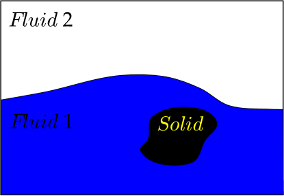
Figure 1: Sketch of a three–phase flow: a surface gravity wave propagation with a submerged body.

The basic features of the problem are sketched in figure 1 with two immiscible fluids separated by an interface and one or more solid bodies. We use the one–fluid formulation of the Navier–Stokes equations and introduce an indicator (or color) function $\mathcal{H}$ to identify the fluids such that $\mathcal{H}$ is $1$ in one fluid and $0$ in the other; the interface is tracked by an additional advection equation for the indicator function. To account for the solid phase, we use the IBM which adds a forcing term to the momentum equation to impose the no–slip boundary condition at the fluid/solid boundary. The full system of equations reads:

$$\nabla\cdot\vec{u}=0$$ (1a)

$$\rho\left(\frac{\partial\vec{u}}{\partial t}+\vec{u}\cdot\nabla\vec{u}\right)=-\nabla p+\nabla\cdot\mathbf{\tau}+\rho\vec{g}+\rho\vec{f}+\vec{f}_{\sigma}$$ (1b)

$$\frac{\partial\mathcal{H}}{\partial t}+\vec{u}\cdot\nabla\mathcal{H}=0$$ (1c)

$$m_{n}\frac{d\vec{V_{n}}}{dt}=\vec{F_{n}}$$ (1d)

$$\frac{d\vec{X_{n}}}{dt}=\vec{V_{n}}$$ (1e)

$$\mathbf{I}_{n}\frac{d\vec{\Omega}_{n}}{dt}=\vec{M}_{n}$$ (1f)

$$\frac{d\vec{\Theta}_{n}}{dt}=\vec{\Omega}_{n}\$$ (1g)

where $\vec{u}$ is the velocity vector, $p$ the pressure, $\rho$ and $\mu$ the density and dynamic viscosity of the fluid, $\mathbf{\tau}$ the viscous stress tensor that for a Newtonian fluid in indicial form is $\tau_{ij}=2\mu D_{ij}=\mu(\partial u_{i}/\partial x_{j}+\partial u_{j}/\partial x_{i})$. $\vec{g}$ is the gravity, $\vec{f}$ the forcing term which enforces the no–slip boundary condition at the immersed boundaries (described in section 3.3) and $\mathcal{H}$ the indicator function. The force $\vec{f}_{\sigma}$ is the surface tension force acting at the interface between the two fluids and directed normal to the interface. The vectors $\vec{X}_{n}$ and $\vec{\Theta}_{n}$ are the linear and angular positions of the center of mass of the $n^{th}$ solid body, while $\vec{V}_{n}$ and $\vec{\Omega}_{n}$ its linear and angular velocity, $\vec{F}_{n}$ and $\vec{M}_{n}$ the external force and moment acting on the body. $m_{n}$ is the mass and $\mathbf{I}_{n}$ the moment of inertia tensor; the subscript $n$ spans all the solid bodies ($1\leq n\leq N$). Note that lower case letters ($u$, $p$, etc.) are used for Eulerian fluid variables while upper case letters ($V$, $X$, etc.) for Lagrangian solid variables.

The fluid properties are constant within each phase and therefore are determined only by the function $\mathcal{H}$, as specified below.

The system (1) has $5$ unknowns for the fluid phases (three velocity components, the pressure and the interface function $\mathcal{H}$) and $12N$ unknowns for the solid phase ($6$ positions and $6$ velocities). The momentum equation (1b) depends on the interface location via the material properties $\rho$ and $\mu$ and on the location of the solid phase via the forcing term $\vec{f}$. The solid body equations (1d)-(1g), instead, depend on the flow field via the loads $\vec{F}_{n}$ and $\vec{M}_{n}$:

$$\vec{F}_{n}=\int_{S_{n}}\left(\mathbf{\tau}\cdot\vec{n}-p\vec{n}\right)\,dS$$ (2a)

$$\vec{M}_{n}=\int_{S_{n}}\left[\left(\mathbf{\tau}\cdot\vec{n}-p\vec{n}\right)\times\vec{r}\right]\,dS$$ (2b)

where $S_{n}$ is the surface of the $n^{th}$ solid body, $\vec{n}$ the local outward normal and $\vec{r}$ the local distance from its center of mass. This makes the equations of the system (1) strongly coupled and some instabilities can arise when integrating them numerically [2]. In the next section we describe the steps to solve the full system of equations.

3 Numerical solver

3.1 Flow solver

We advance in time the momentum equation (1b) by a fractional–step method [6]: first a provisional non–soleinodal velocity field $\vec{u}^{*}$ is computed using an explicit $2^{nd}$ order Adams–Bashfort scheme for the non–linear and viscous terms, yielding the semi–discrete equation for the timestep $l$:

$$\frac{\vec{u}^{*}-\vec{u}^{l}}{\Delta t}=-\frac{1}{\rho^{l+1}}\nabla p^{l}+\frac{3}{2}\vec{H}^{l}-\frac{1}{2}\vec{H}^{l-1}+\vec{g}^{l}+\vec{f}^{l},$$ (3)

where the term $\vec{H}^{l}$ is given by

$$\vec{H}^{l}=-\vec{u}^{l}\cdot\nabla\vec{u}^{l}+\frac{1}{\rho^{l+1}}\nabla\cdot\left(2\mu^{l+1}\mathbf{D}^{l}\right)$$ (4)

with $\mathcal{D}^{l}$ the deformation rate tensor at timestep $l$ $D_{ij}^{l}=(\partial u_{i}^{l}/\partial x_{j}+\partial u_{j}^{l}/\partial x_{i})$ and the material properties $\rho^{l+1}$ and $\mu^{l+1}$ are obtained after the advection of the interface, as described in the next section. The correct velocity field at timestep $l+1$ is obtained by computing a scalar function $\phi$ such that

$$\vec{u}^{l+1}=\vec{u}^{*}-\frac{\Delta t}{\rho^{l+1}}\nabla\phi^{l};$$ (5)

by summing equation (3) and (5) it can be seen that the new pressure is given by

$$p^{l+1}=p^{l}+\phi^{l},$$ (6)

hence $\phi^{l}$ represents the pressure increment at the timestep $l$, that can be computed taking the divergence of equation (5):

$$\nabla\cdot\left(\frac{\Delta t}{\rho^{l+1}}\nabla\phi^{l}\right)=\nabla\cdot\vec{u}^{*}.$$ (7)

This is a variable coefficient Poisson equation because of the presence of the density $\rho^{l+1}$ inside the divergence operator. In order to use FDS, following Dodd & Ferrante,[12], the pressure gradient in the momentum equation is expressed as

$$\frac{\nabla p^{l+1}}{\rho^{l+1}}\rightarrow\frac{\nabla p^{l+1}}{\rho_{0}}+\left(\frac{1}{\rho^{l+1}}-\frac{1}{\rho_{0}}\right)\nabla\hat{p}=\frac{\nabla p^{l}}{\rho_{0}}+\frac{\nabla\phi^{l}}{\rho_{0}}+\left(\frac{1}{\rho^{l+1}}-\frac{1}{\rho_{0}}\right)\nabla\hat{p},$$ (8)

where $\hat{p}$ is an approximation of the pressure $p^{l+1}$ and $\rho_{0}=\min\left(\rho_{1},\rho_{2}\right)$ is a constant density. Using this surrogate for the pressure gradient the momentum equation yields the following relation for the provisional velocity field

$$\frac{\vec{u}^{*}-\vec{u}^{l}}{\Delta t}=-\frac{1}{\rho_{0}}\nabla p^{l}-\left(\frac{1}{\rho^{l+1}}-\frac{1}{\rho_{0}}\right)\nabla\hat{p}+\frac{3}{2}\vec{H}^{l}-\frac{1}{2}\vec{H}^{l-1}+\vec{g}^{l}+\vec{f}^{l},$$ (9)

with the new Poisson equation for the pressure increment

$$\nabla^{2}\phi^{l}=\frac{\rho_{0}}{\Delta t}\nabla\cdot\vec{u}^{*}$$ (10)

and the new velocity correction

$$\vec{u}^{l+1}=\vec{u}^{*}-\frac{\Delta t}{\rho_{0}}\nabla\phi^{l}.$$ (11)

The splitting procedure (8) decouples the pressure gradient from the variable density and allows the use of FDS schemes for the solution of the Poisson equation. Frantzis & Grigoriadis, [14] proposed a local reconstruction of the pressure gradient at the immersed boundaries to avoid the use of points inside the solid regions. However, with the formulation (9)–(11), this is not effective since, while the reconstruction proposed in [14] provides a solenoidal velocity field only in the fluid domain, here the solid phase is moving and information from the solid region would enter anyway the fluid domain because of the dynamics. On the other hand we will see that, because of the fluid/structure interaction, at least two steps (predictor and corrector) and often some iterations are necessary to advance one time interval $\Delta t$, therefore the errors at the immersed boundaries are largely reduced by the multi–step procedure.

It is worth noticing that in the phase with lower density there is no approximation (the last term on the RHS of (8) cancels out) whereas in the phase with the higher density the quality of the approximation depends on how close $\hat{p}$ is to $p^{l+1}$: in the limit $\hat{p}\equiv p^{l+1}$ again there is no approximation. Dodd & Ferrante,[12] have shown that extrapolating $\hat{p}$ from the steps $l$ and $l-1$, that for a constant time step integration corresponds to $\hat{p}=2p^{l}-p^{l-1}$, the approximation (8) preserves the second–order time accuracy of the scheme. Equations (9), (10) and (11) are the steps needed to advance the flow field from timestep $l$ to $l+1$. All the spatial derivatives are approximated by second–order accurate finite–difference scheme except for the viscous terms of equation (4) where the fifth–order WENO is used [32]; this is necessary to avoid oscillations since viscosity jumps are localized across the interface over three grid nodes. Due to the explicit treatment of the non–linear and viscous terms, the timestep is restricted for stability reasons

$$\Delta t=\min\left(CFL\frac{\Delta}{|u_{i}|_{\max}},C_{\nu}\frac{\Delta^{2}}{\nu}\right),$$ (12)

where $\Delta$ is the grid size, $CFL$ the Courant–Friedrichs–Lewy parameter and $C_{\nu}$ a coefficient depending on the number of spatial dimensions ($1/4$ in 2D and $1/6$ in 3D). Note that even though the theoretical $CFL$ condition for the Adams–Bashfort scheme is $CFL\leq 1$, in practice the maximum is $CFL\approx 0.3$ [37]. As it will be shown in the section of the results, this condition can be further restricted for large density ratios bacause of the approximation (8).

3.2 Interface tracking

The method employed for the interface tracking is that proposed in [28], based on the MTHINC originally developed by [19]. Here we briefly describe only the key features of the method and the reader is referred to [28] for a detailed description of the scheme and the relevant validation tests. The cell averaged value of the indicator function $\mathcal{H}$ is defined as the volume fraction of a fluid phase (or volume of fluid, VoF) within a control volume $\delta V$

$$\mathcal{F}\left(\vec{x},t\right)\equiv\frac{1}{\delta V}\int_{\delta V}\mathcal{H}\left(\vec{x},t\right)dV,$$ (13)

being $0\leq\mathcal{F}\left(\vec{x},t\right)\leq 1$. The advection equation for the VoF function is then

$$\frac{\partial\mathcal{F}}{\partial t}+\nabla\cdot\left(\vec{u}\mathcal{H}\right)=\mathcal{F}\vec{u}.$$ (14)

The key point of the MTHINC method is the approximation of the color function by an hyperbolic tangent

$$\mathcal{H}(\vec{X})\approx\hat{\mathcal{H}}(\vec{X})=\frac{1}{2}(1+\text{tanh}(\beta(P(\vec{X})+q))),$$ (15)

where $\vec{X}\in[0,1]$ is a local coordinate system, $\beta$ a sharpness parameter, $q$ a shift and $P$ a three–dimensional surface function which can be either linear (plane) or quadratic (curved surface) at no additional cost. This discretization allows to solve the fluxes of equation (14) by integration of the approximated color function in each computational cell. The material properties of the two fluids are connected to the VoF function $\mathcal{F}$ as follows:

$$\rho(\vec{x},t)=\rho_{1}\mathcal{F}(\vec{x},t)+\rho_{0}(1-\mathcal{F}(\vec{x},t)),$$ (16)

$$\mu(\vec{x},t)=\mu_{1}\mathcal{F}(\vec{x},t)+\mu_{0}(1-\mathcal{F}(\vec{x},t)),$$

where the subscript $1$ stands for phase where $\mathcal{F}$ is equal to $1$ and the subscript $0$ for the other phase. The surface tension force $\vec{f}_{\sigma}$ can be numercially described usgin the Continuum Surface Force method [3] for which $\vec{f}_{\sigma}=\sigma\kappa\nabla\mathcal{H}$, with $\sigma$ the surface tension coefficient and $\kappa$ the local curvature of the interface. The solver has been tested in [28] and recently used in [29, 10].

3.3 Solid boundary treatment

The interaction between the fluid and the solid phases is dealt by the Immersed Boundary method [26]. This technique avoids the use of body conforming meshes by introducing the term $\vec{f}$ in the momentum equation (1b) which enforces the fluid velocity to be equal to that of the solid (no–slip boundary condition). Essentially, the IBM consists of two steps: i) evaluation of the forcing term $\vec{f}$; ii) evaluation of the hydrodynamic loads (2). Several methods have been proposed to implement these two steps, see for example [13, 1, 35, 38, 4, 7]. In the direct forcing approach [13], the term $\vec{f}$ is computed by imposing that the velocity $\vec{u}^{*}$ matches the solid velocity $\vec{V}$ at the solid nodes

$$\frac{\vec{V}^{l+1}-\vec{u}^{l}}{\Delta t}=-\frac{1}{\rho^{l+1}}\nabla p^{l}-\left(\frac{1}{\rho^{l+1}}-\frac{1}{\rho_{0}}\right)\nabla\hat{p}+\frac{3}{2}\vec{H}^{l}-\frac{1}{2}\vec{H}^{l-1}+\vec{g}^{l}+\vec{f}^{l}$$ (17)

which yields for the force

$$\vec{f}^{l}=\frac{\vec{V}^{l+1}-\vec{u}^{l}}{\Delta t}+\frac{1}{\rho^{l+1}}\nabla p^{l}+\left(\frac{1}{\rho^{l+1}}-\frac{1}{\rho_{0}}\right)\nabla\hat{p}-\frac{3}{2}\vec{H}^{l}+\frac{1}{2}\vec{H}^{l-1}-\vec{g}^{l}$$ (18)

with the velocity $\vec{V}^{l+1}$ computed by (1d) and (1f). In practice this corresponds to locally reconstructing the velocity field at the nodes next to the solid boundary (forcing nodes in figure 2(a)). It is worth noticing that, after the correction step (11), which enforces the free divergence of the velocity field, the no–slip boundary condition might be violated. However, it has been shown that, provided the first external node is within the linear part of the boundary layer profile, the error is small and it does not affect significantly the solution [13]. It could be anyway further reduced by iterating between equations (1d), (1f) and (3)-(11) until the desired convergence is achieved.

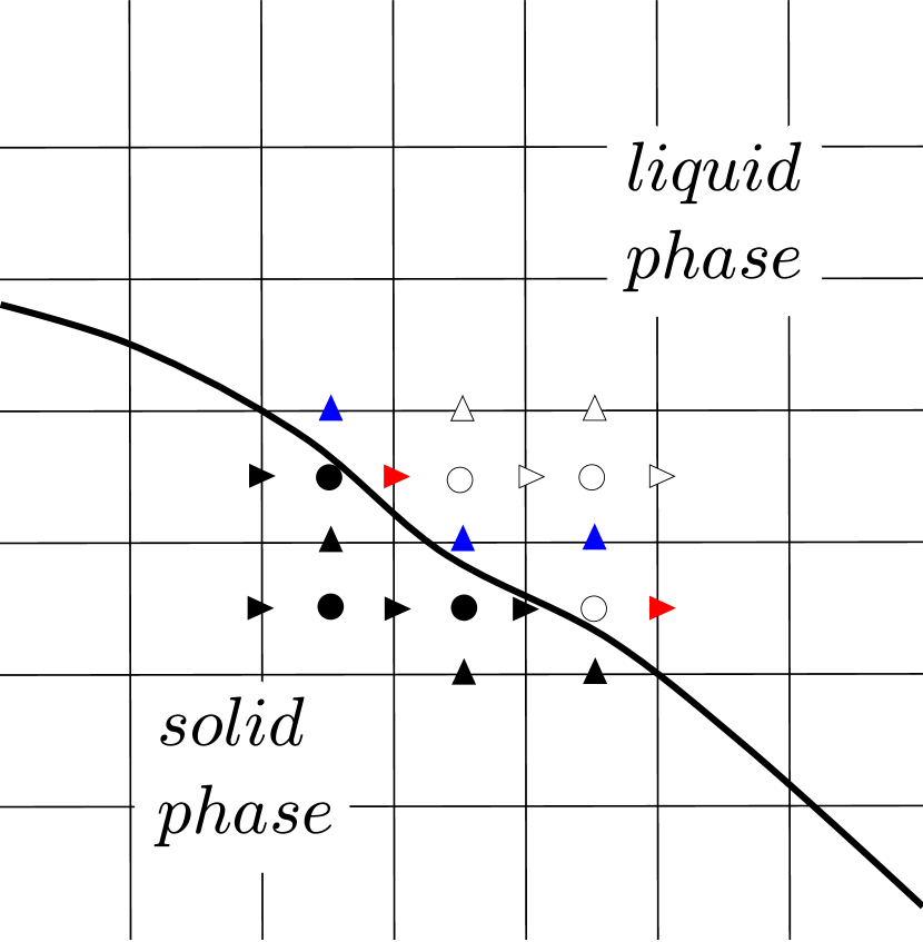
(a)

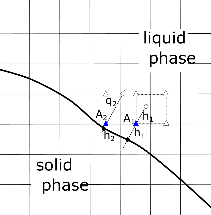
(b)

Figure 2: a) Definition of point tags: solid triangles are velocity solid points, empty triangles are fluid velocity points, red and blue triangles are forcing points for the horizontal and vertical velocity, respectively; solid circles are solid pressure points and empty circles are fluid pressure points. b) Definition of the interpolation stencil: forcing point (blue triangles), auxiliary point (empty diamond), solid boundary point (black diamond).

Since the Cartesian grid does not conform to the solid body, the forcing points do not lie exactly at the boundary, as shown in figure 2(a). For this reason a geometrical description of the solid is required to identify the forcing points and to interpolate the velocity in these points. The proposed scheme has been applied to bodies whose surface could be described by an analytical function since this allows a significant reduction of the computational cost. It is worth mentioning, however, that the method could be easily extended to general complex geometries by using a ray tracing procedure as described in [17].

If, as in the present case, the solid body is a cylinder or a sphere, the geometry is simply defined by the position of the center and a distance from it. We introduce a signed distance function $d$ (positive in the fluid region and negative in the solid) from the surface of the body for every computational node. In the same way we can define the local outward normal, by differentiation of the distance function $\vec{n}=\nabla d$. Starting from the distance field we can tag all the computational velocity points as follows: if $d<0$ the point is solid and tagged with a $0$ flag (black triangles in figure 2(a)). Points where $d\geq 0$ and at least one neighbor with a negative distance are tagged as interface points with a flag $1$ (red and blue triangles in figure 2(a)); all other points with $d>0$ are tagged as fluid with a flag $2$ (empty triangles in figure 2(a)). Pressure points, at the cell center, are tagged only as solid or fluid without the interface flag. For all the interface points the velocity needs to be locally reconstructed in order to apply the no–slip boundary condition. This is done, similarly to [1], by interpolation between the velocity value on the solid body and a virtual point in the fluid domain, as shown in figure 2(b). Starting from the forcing node, following the local normal, a support of $4$ total adjacent points ($8$ in 3D) is constructed. If all the points, except the forcing one, are fluid (as for $A_{1}$ in figure 2(a)) then the auxiliary point is located at a distance $h$ equal to the distance between the forcing node and the solid boundary. The velocity is computed by bi–linear interpolation at the auxiliary point and the desired velocity at the forcing node by linear interpolation between this auxiliary and the boundary nodes (black diamond in figure 2(a)). In case one of the adjacent points is another forcing node (for example $A_{2}$ has as neighbor $A_{1}$), then the auxiliary point is found by intersection of the local normal and the Cartesian grid. The velocity here is computed using the adjacent points and then the velocity on the forcing point is evaluated as done for the previous case. This method provides the value of the velocity $\vec{V}^{l+1}$ on the forcing node to impose the desired boundary condition, and it avoids the inversion of a matrix, as proposed in [41]. Note that the interpolation is performed only for the interface points, while for solid ones the velocity is imposed directly as the solid body velocity $\vec{V}^{l+1}$.

3.4 Hydrodynamic forces and solid body dynamics

The dynamics of the solid phase is governed by the hydrodynamic forces (2) which are computed by integrating over the body surface the integral of viscous stress and pressure. Given that velocity gradients and pressure are not defined exactly at the immersed surface also in this case interpolation is necessary. This is accomplished by considering virtual probes in the fluid domain where $\tau$ and $p$ are computed and then projected along the normal direction onto the surface. Provided the first external point is within the linear part of the boundary layer velocity profile, the viscous stress on the surface is then equal to the value at the probe. Instead, the pressure on the surface is evaluated imposing the boundary condition

$$\frac{\partial p}{\partial n}=-\rho\frac{D\vec{u}}{Dt}\cdot\vec{n}+\rho\vec{g}\cdot\vec{n},$$ (19)

which is obtained by projecting the momentum equation in the wall normal direction. The surface pressure is then

$$p=p_{s}+h_{s}\left(\rho\frac{D\vec{u}}{Dt}\cdot\vec{n}-\rho\vec{g}\cdot\vec{n}\right),$$ (20)

being $p_{s}$ the pressure at the probe and $h_{s}$ the distance between the probe and the immersed surface. The probes are initially located at a distance $\Delta$ from the surface and a support of four nodes (eight in 3D) , as in figure 2(b), is built in the wall normal direction. If these points are all fluid nodes then $\tau$ and $p$ are computed in the probe by bilinear interpolation, otherwise the probe distance is progressively increased by steps of $0.2\Delta$ until the condition on the support is verified. The number of probes is computed by considering a spacing equal to $\Delta$. Once the forces are known, equations (1d)-(1g) are advanced in time using a Hamming $4^{th}$ order modified predictor–corrector method [16], described in appendix Appendix A: Hamming’s $4^{th}$ order modified predictor-corrector.

3.5 Summary of the algorithm

To summarize the algorithm let’s define $\vec{\mathcal{X}}=\left[\vec{X},\vec{\Theta}\right]^{T}$ and $\vec{\mathcal{V}}=\left[\vec{V},\vec{\Omega}\right]^{T}$ the generalized position and velocity for each solid body; for every timestep (after the third), starting from $\vec{u}^{l}$, $p^{l}$, $\mathcal{F}^{l}$, $\vec{\mathcal{X}}^{l}$ and $\vec{\mathcal{V}}^{l}$, the procedure is the following:

1. compute the predicted imporved solution $\left(\vec{\mathcal{X}_{m}}^{l+1},\vec{\mathcal{V}_{m}}^{l+1}\right)$;

2. solve equation (14) to compute $\mathcal{F}^{l+1}$;

3. update fluid properties with (16);

4. compute the provisional velocity field (3);

5. reconstruct the velocity field to impose the no–slip boundary condition given by $\left(\vec{\mathcal{X}_{m}}^{l+1},\vec{\mathcal{V}_{m}}^{l+1}\right)$ on the solid boundary;

6. solve Poisson equation (10) to compute $\phi^{l}$;

7. compute $p^{l+1}$ by (6) and $\vec{u}^{l+1}$ by (11);

8. compute the hydrodynamic loads $\vec{F}^{l}_{1}$ and $\vec{M}^{l}_{1}$ by (2);

9. perform the correction step of the Hamming solver and compute ; $\left(\vec{\mathcal{X}_{1}}^{l+1},\vec{\mathcal{V}_{1}}^{l+1}\right)$;

10. repeat steps from 2. to 9. with boundary condition $\left(\vec{\mathcal{X}_{1}}^{l+1},\vec{\mathcal{V}_{1}}^{l+1}\right)$ for step 5. and check for convergence on $\left(\vec{\mathcal{X}_{k}}^{l+1},\vec{\mathcal{V}_{k}}^{l+1}\right)$;

11. if not converged continue to iterate over steps 2. to 9.;

12. if converged, compute the final solution $\left(\vec{\mathcal{X}}^{l+1},\vec{\mathcal{V}}^{l+1}\right)$ and repeat steps 2. to 8. with this boundary condition for the velocity field.

Note that the strong coupling (i.e. the iterative solver) is necessary only for large density ratio between fluid and solid; in other cases it is possible to use a direct solver performing steps 1-8. When using the strong coupling, the first three timesteps are performed with a forward Euler, Adam-Bashfort 2nd order and Adam-Bashfort 3rd order method, respectively; a tolerance of $10^{-6}$ for convergence is usually small enough for an accurate solution. In case of large acceleration under-relaxation can be used to stabilize the simulation by replacing the force in the corrector step with $F=(1-\chi)F_{k}+\chi F_{k-1}$, with $\chi=[0.1,0.3]$ [8]. For the descirption of the Hamming’s method see appendix A.

4 Results

4.1 Validations

We present here some classical tests either for the immersed boundary method and for its interaction with an interface separating two fluids. We also verify that the method is able to compute the proper energy decay of surface gravity waves and the oscillation period of a submerged pendulum. Note that in all simulations we have set surface tension coefficient to zero to avoid further restrictions on the timestep.

4.1.1 Particle migration

(a)

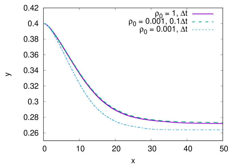
(b)

Figure 3: Lateral migration of a circular particle in a pressure–driven channel at $Re=12.78$ and $96.74$: (a) vertical $vs$ horizontal position; solid line for the present results and symbols for [24]. (b) Effect of the splitting (8): case without splitting (solid purple line), case with splitting and $\Delta t$ ten times smaller (dashed green line), case with splitting and the same $\Delta t$ (dotted blue line).

In the first test case we consider the migration of a neutrally buoyant particle in a two–dimensional pressure–driven Poiseuille flow [24]. The motion of the particle is a consequence of pressure distribution, inertia and rotational lift; an accurate evaluation of the forces is necessary to properly simulate the particle dynamics. We consider a square domain of size $L=1$, periodic in the horizontal direction and vertically bounded by two solid walls. Initially the flow is at rest and a pressure gradient is applied in the horizontal direction. The circular particle has a radius of $0.125L$ and it is initially located at a vertical distance of $0.4L$ from the lower plate. Two different cases are considered by varying the viscosity of the fluid $\mu$, which correspond to two different Reynolds numbers, namely $Re=12.78$ and $96.74$. The Reynolds number is based on the space–averaged inlet velocity $\tilde{u}$ and the size of the domain $L=1$, i.e. $Re=\rho L\tilde{u}/\mu$, the density of the particle $\rho_{p}$ is the same as that of the fluid $\rho$. For the lower value of $Re$ we use a grid of $96\times 96$ points while for the higher $Re$ the grid is $192\times 192$. The particle migrates from the initial to an equilibrium position close to the lower wall, as shown in figure 3(a). A good agreement for both Reynolds numbers, with the results of [24], is found.

To show the effect of the splitting procedure (8) we simulate the case at $Re=12.78$ by introducing a minimum density equal to $\rho_{0}=0.001$, which corresponds to a case with two fluids with density ratio 0.001, so that the term involving $\hat{p}$ is non-zero. Due to the small value of $\rho_{0}$, it is necessary to decrease the timestep in order to recover the approximation between $\hat{p}$ and $p^{l+1}$, as clearly shown in figure 3(b). The timestep restriction depends on the density ratio and we have found that a reduction of $10$ times for a density ratio of $0.001$ is enough while for bigger density ratios, for example $0.01$, already halving the timestep yields the correct time evolution of the particle. This is consistent with the results of [14]. For this test the direct solver is stable and it is not necessary to use the iterative solver.

4.1.2 Water exit

(a)

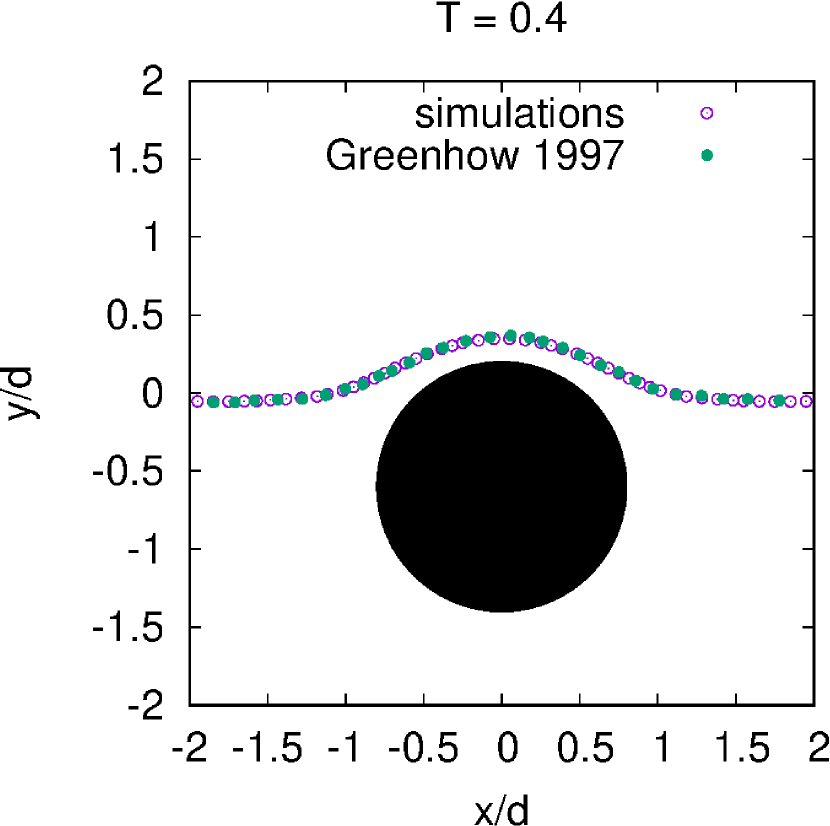
(b)

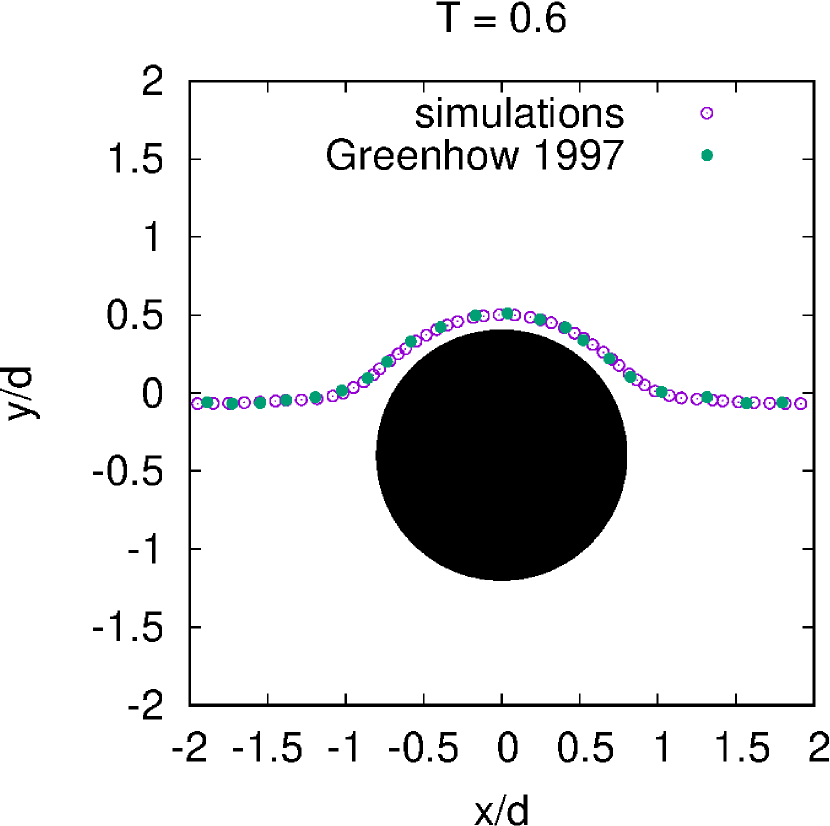
(c)

Figure 4: Water exit test case: a) sketch of the computational domain; b)-c) interface deformation with $\epsilon=0.8$ and $Fr=0.39$: present results (open circles), data from [15] (solid circles); lengths are made non–dimensional by the initial distance $d$.

The next test case consists of a cylinder rising close to the interface separating water and air, as in [15]. The cylinder has radius $a$, it is at a distance $d$ below the still water level, and rises with a constant velocity $V$. The inviscid problem is governed by two nondimensional parameters, $\epsilon=a/d=0.8$ and the Froude number $Fr=V/\sqrt{gd}=0.39$, with $g$ the acceleration of gravity. The material properties ratio is that of water and air, i.e. $\rho_{w}/\rho_{a}=850$ and $\mu_{w}/\mu_{a}=1.92\text{x}10^{-2}$. Note that the reference solution of [15] has been derived from the potential theory for inviscid fluids; the present solver, instead, is designed for viscous flows therefore we have selected a Reynolds number high enough to minimize viscous effects but, at the same time, small enough to limit the computational effort. In the real air/water case it results $Re\approx{\cal O}(10^{5})$; here we have set the water viscosity so to have a Reynolds number $Re=\rho_{w}Va/\mu_{w}=1000$ which proved to be enough for our purposes. The domain is $40a$ wide and $20a$ high, with a water depth of $16a$ and it is discretized by a grid of $4096\times 2048$ points. We compare our results with the numerical ones proposed by [15], reported in figure 4 at fixed non–dimensional times of $T=tV/d=0.4$ and $0.6$. The results, in terms of interface deformation, are in very good agreement with those of [15]. Also for this test the direct solver is enough stable and it is not necessary to use the iterative solver.

4.1.3 Viscous damping of surface gravity waves

Surface gravity waves propagating in inviscid fluids can be described using the potential theory which yields an irrotational velocity field. For viscous fluids, instead, there is an additional rotational flow given by the presence of the boundary layer at the free–surface. For waves of small amplitude, i.e. waves for which $a<<\lambda$, with $a$ the wave amplitude and $\lambda$ its wavelength, the rotational flow is confined in a small layer across the surface while the rest of the flow can be still described by the potential theory. Under this assumption the total wave energy decay in time, given by the sum of the kinetic and potential contributions, can be computed from the potential theory (see Landau & Lifshitz, [22] chapter II section 25) and it results in an exponential decay of the form $E(t)=E(t=0)e^{-2\gamma t}$ with the coefficient $\gamma=2\nu k^{2}$, being $\nu$ the kinematic viscosity of the fluid and $k=2\pi/\lambda$ the wavenumber. The kinetic energy contribution is given by

$$E_{k}(t)=\int_{0}^{\lambda}\int_{-h}^{\eta}\frac{1}{2}\rho\vec{u}^{2}\,dxdy$$ (21)

with $h$ the fluid depth at rest and $\eta$ the free–surface level with respect to the equilibrium position ($z=0$). The potential energy is

$$E_{p}(t)=\int_{0}^{\lambda}\int_{-h}^{\eta}\rho gz\,dxdy-E_{p0}$$ (22)

with $E_{p0}=\int_{0}^{\lambda}\int_{-h}^{0}\rho gz\,dxdy=-\rho g\lambda h^{2}/2$ the potential energy of the still water level. We simulate the propagation of a surface gravity wave of wavelength $\lambda$ in a periodic square box of size $\lambda$ with a fluid depth of $h=\lambda/2$ and a steepness $\varepsilon=ak=0.05$. The density and viscosity ratios are those of water and air, $1/850$ and $1.96\text{x}10^{2}$, respectively, while the Reynolds number based on the phase velocity $c_{f}=\sqrt{g\lambda}$ and on the wavelength $\lambda$ is $Re=g^{0.5}\lambda^{3/2}/\nu=1.0\text{x}10^{4}$. The initial conditions for the surface elevation $\eta$ and the velocity field $\vec{u}=(u,w)$ are given by the linear theory:

$$\eta(x,0) =a\cos\left(kx\right),$$ (23a)

$$u(x,y,0) =\left(1-\mathcal{H}\right)a\omega e^{ky}\cos\left(kx\right)-\mathcal{H}a\omega e^{-ky}\cos\left(kx\right),$$ (23b)

$$v(x,y,0) =\left(1-\mathcal{H}\right)a\omega e^{ky}\sin\left(kx\right)+\mathcal{H}a\omega e^{-ky}\sin\left(kx\right),$$ (23c)

with $\mathcal{H}=0$ for the water and $\mathcal{H}=1$ in the air. For stability reason the initial VoF function $\mathcal{H}$ is filtered one time using bilinear interpolation. In figure 5 (left) we report the vorticity contours after one period, which clearly shows its concentration in a small layer below the water surface; in the right panel we show the energy decay in time computed by equations (21)-(22) alongside the theoretical exponential decay with excellent agreement. The simulation has been performed on a grid of $256\times 256$ points.

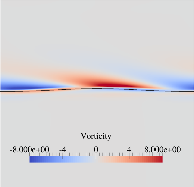
Figure 5: (Left panel) Vorticity contours after one wave period; (Right panel) Comparison of the energy decay between the computed values from equations (21)-(22) and the theoretical exponential decay.

4.1.4 Frequency oscillations of a submerged reversed pendulum

Figure 6: Oscillation frequency of a submerged reversed pendulum: (left) time history of the horizontal position of the center of mass for one case with $\rho=400$, symbols highlight the maxima and minima used for the computation of the period; (right) comparison of the computed frequency with equations (24) and (25).

We considere here a 2D reversed pendulum, i.e. a cylinder lighter than ther surrounding fluid and anchored at the bottom. The natural frequency of a simple pendulum, for small oscillation amplitude, is given by $\omega=\sqrt{g/\ell}$, with $g$ the gravity and $\ell$ the distance of the center of rotation from the center of mass, and is obtained by a balance between the tension of the contraint and the weight. On account also of the buoyancy force the frequency becomes

$$\omega=\sqrt{\frac{g(\rho-\rho_{p})}{\ell\rho_{p}}},$$ (24)

where $\rho$ is the density of the surrounding fluid and $\rho_{p}$ that of the pendulum. This relation is appropriate when the pendulum is much denser than the fluid whereas in the general case it is necessary to take into account also the added mass:

$$\omega=\sqrt{\frac{g}{\ell}\frac{\rho-\rho_{p}}{\rho_{p}+c\rho}}$$ (25)

with $c$ the added mass coefficient depending on the shape of the swinging mass (for example $c=0.5$ for spheres and $c=1$ for cylinders). Here we compute the oscillation frequency for a cylinder (2D case) for different values of the density $\rho$ and compare the results with equations (24) and (25). To this end, we give an initial displacement to the center of mass of the cylinder from the equilibrium position and let the pendulum oscillate; after $10$ periods we compute the time difference between all maxima and minima of the horizontal position of the pendulum (as in figure 6). In figure 6b we compare the computed frequency of the pendulum with equations (24) and (25): the results show that including the added mass term gives a good approximation of the evaluations of the pendulum frequency, with an error about 5%.

The simulations are performed with the following setup: radius of the pendulum $r=1$, fluid density $\rho=1000$, fluid viscosity $\mu=2.6\text{x}10^{-3}$, pendulum length $\ell=1.8r$, size of the domain $10r\text{x}10r$; the grid has $256\times 256$ points. The iterative solver has been used with a tolerance of $10^{-6}$.

4.2 Applications

4.2.1 Surface gravity wave propagating over a submerged reversed pendulum

We study now the interaction between surface gravity waves propagating over a submerged reversed pendulum. The wave has wavelength $\lambda$ and propagates with a phase velocity $c_{p}$ from the left to the right. The pendulum of radius $r$, is located (at rest) at a distance $d$ from the still water level and it is anchored at a distance $\ell$ from its center of mass. The density of the pendulum $\rho_{p}$ is smaller than the water density $\rho_{w}$, the buoyancy pulls the cylinder upwards and the constraint is always under positive tension. From the linear theory, the frequency of the wave is

$$\omega_{w}=\sqrt{gh\tanh{kh}},$$ (26)

with $g$ the gravitational acceleration, $k=2\pi/\lambda$ the wavenumber and $h$ the depth of the still water level. The frequency of the pendulum can be estimated using equation (25).

The problem depends on several parameters, which make the analysis quite complicated; here we show one case with the following setup:

$\lambda/r$	$h/r$	$\ell/r$	$d/r$	$\rho_{p}/\rho_{w}$	$\rho_{a}/\rho_{w}$	$\mu_{a}/\mu_{w}$	$\varepsilon=ak$	$Re$
33.615	8.40375	2.5	1.65	0.8	1/850	1.96e-2	0.05	$10^{5}$

with the Reynolds number defined as $Re=\rho_{w}\lambda^{3/2}g^{1/2}/\mu_{w}$. Note that with this choice of the parameters the period of the pendulum is $1.6$ times that of the wave. The domain is wide $\lambda$ and high $0.5\lambda$, the pendulum is located at the center of the domain in the horizontal direction; the initial wave profile is

$$\eta(x,0)=a\cos(kx),$$ (27)

while the initial velocity field in the water is

$$u(x,y,0)=a\omega\frac{\cosh\left(k\left(y+h\right)\right)}{\sinh\left(kh\right)}\cos\left(kx\right),$$ (28a)

$$v(x,y,0)=a\omega\frac{\sinh\left(k\left(y+h\right)\right)}{\sinh\left(kh\right)}\sin\left(kx\right)$$ (28b)

and in the air the velocity has the same expression except for a change of sign in $y$. To ensure that the cord is always at the maximum extension, i.e. $\ell$ is a rigid constraint; accordingly we compute the hydrodynamic forces and then solve for the rotation around the fulcrum of the pendulum; velocity and position of the center of mass are then computed from the angular quantities. Hence, there is no rotation of the pendulum around its center of mass.

The wave induces an oscillatory motion of the pendulum, as shown in figure 7(a). Since the wave period is different from that of the pendulum, the dynamics is characterised by different oscillation frequencies. Figures 7(b)-7(c)-7(d) exhibit the contour of the horizontal velocity, the interface location and the pendulum position at four time instants, corresponding to the black dots in figure 7(a). Based on the location of the pendulum with respect to the phase of the velocity field, pendulum and wave can be in phase or out of phase. The small peaks in the position, for example, correspond to instants in which the pendulum has a negative velocity and interacts with the positive phase velocity of the wave, as shown in figure 7(c).

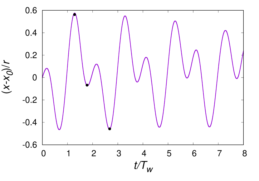
(a)

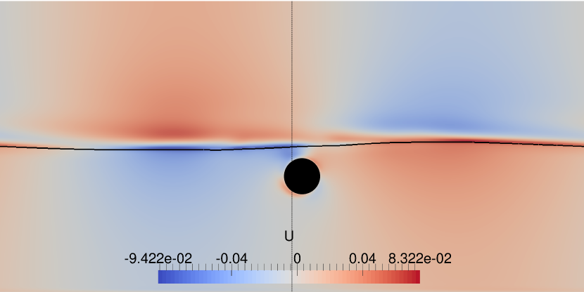
(b)

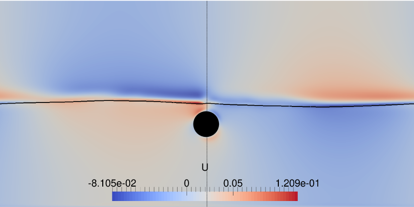
(c)

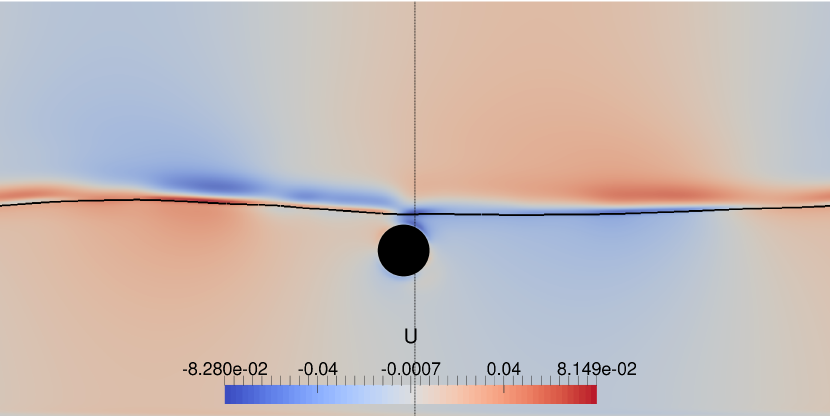
(d)

Figure 7: Surface gravity wave propagating over a submerged pendulum. (a) horizontal position of the pendulum; black dots are the instants for other panels. (b)-(d) color map of horizontal velocity, position of the pendulum and of the interface (the line has been made thicker in the sake of clarity), corresponding to the black dots in panel (a) with time increasing from top left to bottom right. The entire domain is represented.

One interesting aspect of the problem is the energy transfer between the wave and the pendulum. We report in figure 8(a) the time history of the kinetic and potential energy, computed by equations (21) and (22), for the cases with and without pendulum. For this case the wave potential energy at rest is computed only in the fluid domain, i.e. $E_{p0}=\rho_{w}g(-\lambda h^{2}/2+d\pi r^{2})$, with $d$ varying in time. The presence of the pendulum induces strong oscillations in the wave energy components, both the kinetic and the potential, which implies a continuous energy transfer between the wave and the pendulum. When the wave is out of phase with the pendulum, the solid opposes to the wave and induces an increase in the wave height (as in figure 8(c)) which corresponds to an increase in the potential energy of the wave. This energy then goes into kinetic energy with a strong reduction of the potential contribution, which in some instant drops almost to zero, corresponding to a small wave amplitude. The energy is then dissipated in the fluid by vorticity production and the system has an overall higher energy dissipation in time, as clearly shown in figure 8(b).

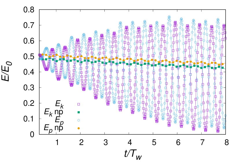
(a)

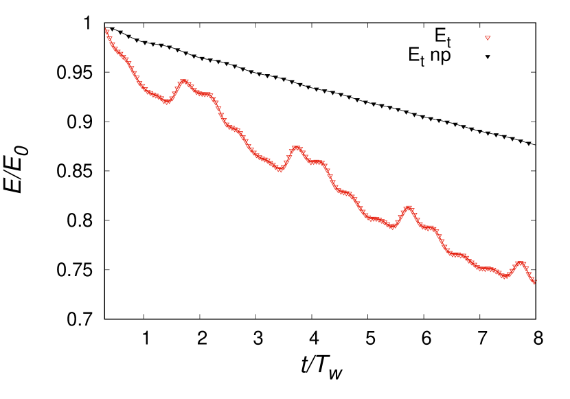
(b)

(c)

(d)

Figure 8: Surface gravity wave propagating over a submerged pendulum. (a) time history of wave energy components for the case with and without pendulum: wave kinetic energy with pendulum (purple open square), wave potential energy with pendulum (blue open circles), wave kinetic energy without pendulum (green solid square), wave potential energy without pendulum (orange solid circles). (b) Total wave energy for the case with pendulum (black solid triangles) and without pendulum (red open triangles). All terms are normalized by the initial total energy. (c)–(d) comparison of the surface profile between the case with pendulum (solid line, labeled as wp) and without (dashed line, labeled np). Dotted line represents the still water level.

4.3 3D wave breaking induced by a submerged body

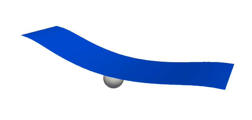
(a)

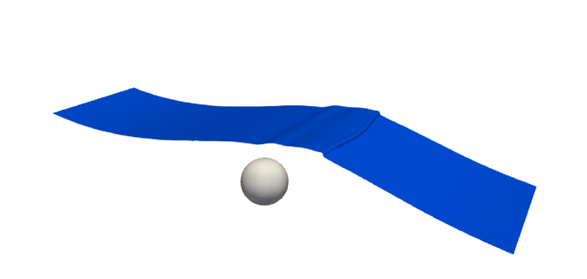
(b)

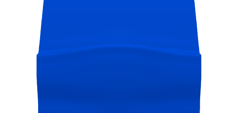
(c)

(d)

Figure 9: 3D surface wave breaking: interface location at $T=0$ (a) and at $T=0.5$ (b); the wave propagates from the left to the right. Detailed view of the breagkin front from top (c). Wave profile in a $x-y$ plane located at the center in the $z$ direction (d).

Finally we want to show a three–dimensional application of the solver. Wave breaking is an important phenomenon which occurs in ocean and heavily affects the air–water mass and energy exchanges. It has been extensively studied in the last decades and several criteria have been proposed in order to predict the onset of wave breaking [25]. Here we want to show the effect of a submerged body on the breaking of a surface gravity wave. To this aim we simulate a third–order Stokes wave

$$\eta(x)=\frac{a}{\lambda}\left(\cos(kx)+\frac{1}{2}\varepsilon\cos(2kx)+\frac{3}{8}\varepsilon^{2}\cos(3kx)\right),$$ (29)

which, for a high enough value of the initial steepness $\varepsilon=2\pi a/\lambda$ (about 0.32), leadto wave breaking [5, 18, 11]. The submerged body is a sphere of radius $r=0.05\lambda$ located at a distance $d=0.1$ below the still water level; the initial velocity field is derived from the linear theory and the Reynolds number, based on the wavelength $\lambda$ and phase speed $c=\sqrt{g\lambda}$, is set to $Re=\rho\lambda\sqrt{g\lambda}/\mu=40000$. In this simulation the initial steepness is $\varepsilon=0.25$ which corresponds to a non–breaking case [18, 11]. However, the presence of the sphere produces a breaking front on the surface which is a spilling breaking, as found for larger values of the steepness. The sphere produce a disturbance on the surface and when the wave crest reaches the location of the sphere (figure 9 d), it induces an increase in the local height which corresponds to a steepness rise. If this perturbation is strong enough to overcome the limiting steepness, wave breaking occurs, as clearly shown in figure 9(b). The simulation has been performed in a domain of size $\lambda\times\lambda\times\lambda/4$ with a resolution $256$ nodes per wavelength and a computational time of 1 hour per wave period on 512 processors Intel Xeon E5-2697 v4 at 2.30 GHz.

5 Conclusions

A fully Eulerian solver for the solution of multiphase flows with solid bodies is presented which allows an efficient parallelization of the solver. The solid phase is described by an immersed body formulation with a direct forcing approach and an interpolated procedure for the reconstruction of the velocity field close to the solid boundary. The rigid body motion is coupled with the fluid solver through a 4th order predictor corrector method which allows for stable simulations in presence of large oscillations or solids lighter than the surrounding fluid, for which the added mass play an important role. In this case also underelxation could be used to stabilize the simulation. The hydrodynamic loads are computed by means of probes located in the fluid domain close to the forcing nodes and their accurate computation is crucial for a proper evaluation of the solid body dynamics. The two fluids phase are simulated by a volume of fluid solver coupled with the splitting method for the constant coefficient Poisson solver. The immersed boundary method do not pose any restriction on the timestep by its coupling with the splitting procedure require a decrease of the timestep for large density ratio beween the fluid and the solid phase while no restriction is found for buoyancy free bodies. The solver is validated with some test cases available in literature as migration of particle in pressure–driven flow, water exit of a cylidner and the frequency oscillation of a sumberged reversed pendulum. Excellent agreement has been found for all test cases. The method is also applied to a case of a surface gravity wave propagating over a submerged pendulum and the 3D spilling breaking induced by a submerged sphere. The method can be applied to solid body of arbitraty shape by replacing the distance function for the solid geometry description with a ray tracing algorithm. Extension to deformable bodies could be done by replacing the direct forcing apporach with a moving least square method and wil be the subject of future work as for the contact angle between the solid and the liquid.

Appendix A: Hamming’s $4^{th}$ order modified predictor-corrector

At each timestep, once the forces are known, equations (1d)-(1g) are advanced in time using a Hamming’s 4th order modified predictor-corrector method [16]. Defining $\vec{\mathcal{X}}=\left[\vec{X},\vec{\Theta}\right]^{T}$ the unknown vector for the position and $\vec{\mathcal{V}}=\left[\vec{V},\vec{\Omega}\right]^{T}$ the unknown vector for the velocity, the evolution is computed by the following steps

1. Predictor step: evaluate the predicted solution $\left(\mathcal{X}^{l+1}_{p},\mathcal{V}^{l+1}_{p}\right)$ at timestep $n+1$

   • $\vec{\mathcal{A}}^{l}=\vec{F}^{l}/m$

   • $\vec{\mathcal{V}}^{l+1}_{p}=\vec{\mathcal{V}}^{l-3}+\frac{4}{3}\Delta t\left(2\vec{\mathcal{A}}^{l}-\vec{\mathcal{A}}^{l-1}+2\vec{\mathcal{A}}^{l-2}\right)$

   • $\vec{\mathcal{X}}^{l+1}_{p}=\vec{\mathcal{X}}^{l-3}+\frac{4}{3}\Delta t\left(2\vec{\mathcal{V}}^{l}-\vec{\mathcal{V}}^{l-1}+2\vec{\mathcal{V}}^{l-2}\right)$

   improve it with an estimation of the error at previous timestep

   • $\vec{\mathcal{V}}^{l+1}_{m}=\vec{\mathcal{V}}^{l+1}_{p}-\frac{112}{121}\left(\vec{\mathcal{V}}^{l}_{p}-\vec{\mathcal{V}}^{l}\right)$

   • $\vec{\mathcal{X}}^{l+1}_{m}=\vec{\mathcal{X}}^{l+1}_{p}-\frac{112}{121}\left(\vec{\mathcal{X}}^{l}_{p}-\vec{\mathcal{X}}^{l}\right)$

   and solve flow equations using as boundary condition $\left(\mathcal{X}^{l+1}_{m},\mathcal{V}^{l+1}_{m}\right)$ to evaluate $F^{l+1}_{1}$.

2. Corrector step: correct the solution iteratively (loop on $k$, starting from $k=1$)

   • $\vec{\mathcal{A}}^{l+1}_{k}=\vec{F}^{l+1}_{k}/m$

   • $\vec{\mathcal{V}}^{l+1}_{k}=\frac{1}{8}\left(9\vec{\mathcal{V}}^{l}-\vec{\mathcal{V}}^{l-2}\right)+\frac{3}{8}\Delta t\left(2\vec{\mathcal{A}}^{l+1}_{k}+2\vec{\mathcal{A}}^{l}-\vec{\mathcal{A}}^{l-1}\right)$

   • $\vec{\mathcal{X}}^{l+1}_{k}=\frac{1}{8}\left(9\vec{\mathcal{X}}^{l}-\vec{\mathcal{X}}^{l-2}\right)+\frac{3}{8}\Delta t\left(2\vec{\mathcal{V}}^{l+1}_{k}+2\vec{\mathcal{V}}^{l}-\vec{\mathcal{V}}^{l-1}\right)$

   and check for convergence: $\min\left(\vec{|\mathcal{X}}^{l+1}_{k}-\vec{\mathcal{X}}^{l+1}_{k-1}|,|\vec{\mathcal{V}}^{l+1}_{k}-\vec{\mathcal{V}}^{l+1}_{k-1}|\right)<\epsilon$, where the values at $k=0$ are the modified value of the predictor step and $\epsilon$ is the tolerance. If converged, make the final correction to the solution:

   • $\vec{\mathcal{V}}^{l+1}=\vec{\mathcal{V}}^{l+1}_{k}+\frac{9}{121}\left(\vec{\mathcal{V}}^{l+1}_{p}-\vec{\mathcal{V}}^{l+1}_{k}\right)$

   • $\vec{\mathcal{X}}^{l+1}=\vec{\mathcal{X}}^{l+1}_{k}+\frac{9}{121}\left(\vec{\mathcal{X}}^{l+1}_{p}-\vec{\mathcal{X}}^{l+1}_{k}\right)$

   and solve flow equations with boundary condition $\left(\mathcal{X}^{l+1},\mathcal{V}^{l+1}\right)$. If not converged, solve flow equations with boundary condition $\left(\mathcal{X}^{l+1}_{k},\mathcal{V}^{l+1}_{k}\right)$, evaluate $F^{l+1}_{k}$ and then repeat the corrector step until convergence.

References

- Balaras, [2004] Balaras, Elias. 2004. Modeling complex boundaries using an external force field on fixed Cartesian grids in large-eddy simulations. Computers and Fluids, 33(3), 375–404.
- Borazjani et al. , [2008] Borazjani, Iman, Ge, Liang, & Sotiropoulos, Fotis. 2008. Curvilinear immersed boundary method for simulating fluid structure interaction with complex 3D rigid bodies. Journal of Computational Physics, 227(16), 7587–7620.
- Brackbill et al. , [1992] Brackbill, J. U., Kothe, D. B., & Zemach, C. 1992. A continuum method for modeling surface tension. Journal of Computational Physics, 100(2), 335–354.
- Breugem, [2012] Breugem, Wim Paul. 2012. A second-order accurate immersed boundary method for fully resolved simulations of particle-laden flows. Journal of Computational Physics, 231(13), 4469–4498.
- Chen et al. , [1999] Chen, Gang, Kharif, Christian, Zaleski, Stéphane, & Li, Jie. 1999. Two-dimensional Navier-Stokes simulation of breaking waves. Physics of Fluids, 11(1), 121–133.
- Chorin, [1967] Chorin, Alexandre Joel. 1967. A numerical method for solving incompressible viscous flow problems. Journal of Computational Physics, 2(1), 12–26.
- de Tullio & Pascazio, [2016] de Tullio, M. D., & Pascazio, G. 2016. A moving-least-squares immersed boundary method for simulating the fluid–structure interaction of elastic bodies with arbitrary thickness. Journal of Computational Physics, 325, 201–225.
- de Tullio et al. , [2009] de Tullio, M. D., Cristallo, A., Balaras, E., & Verzicco, R. 2009. Direct numerical simulation of the pulsatile flow through an aortic bileaflet mechanical heart valve. Journal of Fluid Mechanics, 622, 259–290.
- De Vita et al. , [2016] De Vita, F., de Tullio, M. D., & Verzicco, R. 2016. Numerical simulation of the non-Newtonian blood flow through a mechanical aortic valve: Non-Newtonian blood flow in the aortic root. Theoretical and Computational Fluid Dynamics, 30(1-2), 129–138.
- De Vita et al. , [2019] De Vita, Francesco, Rosti, Marco Edoardo, Caserta, Sergio, & Brandt, Luca. 2019. On the effect of coalescence on the rheology of emulsions. Journal of Fluid Mechanics, 880, 969–991.
- Deike et al. , [2015] Deike, Luc, Popinet, Stephane, & Melville, W. Kendall. 2015. Capillary effects on wave breaking. Journal of Fluid Mechanics, 769, 541–569.
- Dodd & Ferrante, [2014] Dodd, Michael S., & Ferrante, Antonino. 2014. A fast pressure-correction method for incompressible two-fluid flows. Journal of Computational Physics, 273, 416–434.
- Fadlun et al. , [2000] Fadlun, E. A., Verzicco, R., Orlandi, P., & Mohd-Yusof, J. 2000. Combined Immersed-Boundary Finite-Difference Methods for Three-Dimensional Complex Flow Simulations. Journal of Computational Physics, 161(1), 35–60.
- Frantzis & Grigoriadis, [2019] Frantzis, C., & Grigoriadis, D. G.E. 2019. An efficient method for two-fluid incompressible flows appropriate for the immersed boundary method. Journal of Computational Physics, 376, 28–53.
- Greenhow & Moyo, [1997] Greenhow, Martin, & Moyo, Simiso. 1997. Water entry and exit of horizontal circular cylinders. Philosophical Transactions of the Royal Society A: Mathematical, Physical and Engineering Sciences, 355(1724), 551–563.
- Hamming, [1959] Hamming, R. W. 1959. Stable Predictor-Corrector Methods for Ordinary Differential Equations. 6(1), 37–47.
- Iaccarino & Verzicco, [2003] Iaccarino, Gianluca, & Verzicco, Roberto. 2003. Immersed boundary technique for turbulent flow simulations. Applied Mechanics Reviews, 56(3), 331–347.
- Iafrati, [2009] Iafrati, A. 2009. Numerical study of the effects of the breaking intensity on wave breaking flows. Journal of Fluid Mechanics, 622, 371–411.
- Ii et al. , [2012] Ii, Satoshi, Sugiyama, Kazuyasu, Takeuchi, Shintaro, Takagi, Shu, Matsumoto, Yoichiro, & Xiao, Feng. 2012. An interface capturing method with a continuous function: The THINC method with multi-dimensional reconstruction. Journal of Computational Physics, 231(5), 2328–2358.
- Kim & Moin, [1985] Kim, J., & Moin, P. 1985. Application of a fractional-step method to incompressible Navier-Stokes equations. Journal of Computational Physics, 59(2), 308–323.
- Kim et al. , [2001] Kim, Jungwoo, Kim, Dongjoo, & Choi, Haecheon. 2001. An Immersed-Boundary Finite-Volume Method for Simulations of Flow in Complex Geometries. Journal of Computational Physics, 171(1), 132–150.
- Landau & Lifshitz, [1959] Landau, L. D., & Lifshitz, E. M. 1959. Fluid Mechanics. Pergamon Press.
- Lee et al. , [2011] Lee, Jongho, Kim, Jungwoo, Choi, Haecheon, & Yang, Kyung-Soo. 2011. Sources of spurious force oscillations from an immersed boundary method for moving-body problems. Journal of Computational Physics, 230(7), 2677 – 2695.
- Pan & Glowinski, [2002] Pan, Tsorng Whay, & Glowinski, Roland. 2002. Direct simulation of the motion of neutrally buoyant circular cylinders in plane poiseuille flow. Journal of Computational Physics, 181(1), 260–279.
- Perlin et al. , [2013] Perlin, Marc, Choi, Wooyoung, & Tian, Zhigang. 2013. Breaking Waves in Deep and Intermediate Waters. Annual Review of Fluid Mechanics, 45(1), 115–145.
- Peskin, [1972] Peskin, Charles S. 1972. Flow patterns around heart valves: a numerical method. Journal of computational physics, 10(2), 252–271.
- Popinet, [2009] Popinet, Stéphane. 2009. An accurate adaptive solver for surface-tension-driven interfacial flows. Journal of Computational Physics, 228(16), 5838–5866.
- Rosti et al. , [2018] Rosti, Marco E., De Vita, Francesco, & Brandt, Luca. 2018. Numerical simulations of emulsions in shear flows. Acta Mechanica, 230(2), 667–682.
- Rosti et al. , [2019] Rosti, Marco E., Ge, Zhouyang, Jain, Suhas S., Dodd, Michael S., & Brandt, Luca. 2019. Droplets in homogeneous shear turbulence. Journal of Fluid Mechanics, 876, 962–984.
- Scardovelli & Zaleski, [1999] Scardovelli, Ruben, & Zaleski, Stéphane. 1999. Direct numerical simulation of free-surface and interfacial flow. Annual review of fluid mechanics, 31(1), 567–603.
- Sethian, [1999] Sethian, James Albert. 1999. Level set Methods and Fast Marching Methods: Evolving interfaces in geometry, fluid mechanics, computer vision, and materials science. Cambridge university press Cambridge.
- Shu, [2009] Shu, Chi-Wang. 2009. High Order Weighted Essentially Nonoscillatory Schemes for Convection Dominated Problems. SIAM Review, 51(1), 82–126.
- Swarztrauber, [1977] Swarztrauber, Paul N. 1977. The methods of cyclic reduction, Fourier analysis and the FACR algorithm for the discrete solution of Poisson’s equation on a rectangle. Siam Review, 19(3), 490–501.
- Tryggvason et al. , [2011] Tryggvason, Grétar, Scardovelli, Ruben, & Zaleski, Stéphane. 2011. Direct numerical simulations of gas–liquid multiphase flows. Cambridge University Press.
- Uhlmann, [2005] Uhlmann, Markus. 2005. An immersed boundary method with direct forcing for the simulation of particulate flows. Journal of Computational Physics, 209(2), 448–476.
- Unverdi & Tryggvason, [1992] Unverdi, Salih Ozen, & Tryggvason, Grétar. 1992. A front-tracking method for viscous, incompressible, multi-fluid flows. Journal of computational physics, 100(1), 25–37.
- van der Poel et al. , [2015] van der Poel, Erwin P., Ostilla-Mónico, Rodolfo, Donners, John, & Verzicco, Roberto. 2015. A pencil distributed finite difference code for strongly turbulent wall-bounded flows. Computers and Fluids, 116, 10–16.
- Vanella & Balaras, [2009] Vanella, Marcos, & Balaras, Elias. 2009. A moving-least-squares reconstruction for embedded-boundary formulations. Journal of Computational Physics, 228(18), 6617–6628.
- Vanella et al. , [2014] Vanella, Marcos, Posa, Antonio, & Balaras, Elias. 2014. Adaptive mesh refinement for immersed boundary methods. Journal of Fluids Engineering, Transactions of the ASME, 136(4), 1–9.
- Viola et al. , [2020] Viola, Francesco, Meschini, Valentina, & Verzicco, Roberto. 2020. Fluid–Structure-Electrophysiology interaction (FSEI) in the left-heart: A multi-way coupled computational model. European Journal of Mechanics - B/Fluids, 79, 212 – 232.
- Yang & Balaras, [2006] Yang, Jianming, & Balaras, Elias. 2006. An embedded-boundary formulation for large-eddy simulation of turbulent flows interacting with moving boundaries. Journal of Computational Physics, 215(1), 12–40.
- Yang & Stern, [2009] Yang, Jianming, & Stern, Frederick. 2009. Sharp interface immersed-boundary/level-set method for wave-body interactions. Journal of Computational Physics, 228(17), 6590–6616.