On the interplay between mobility and hospitalization capacity during the COVID-19 pandemic: The SEIRHUD model
Abstract
Measures to reduce the impact of the COVID-19 pandemic require a mix of logistic, political and social capacity. Depending on the country, different approaches to increase hospitalization capacity or to properly apply lock-downs are observed. In order to better understand the impact of these measures we have developed a compartmental model which, on the one hand allows to calibrate the reduction of movement of people within and among different areas, and on the other hand it incorporates a hospitalization dynamics that differentiates the available kinds of treatment that infected people can receive. By bounding the hospitalization capacity, we are able to study in detail the interplay between mobility and hospitalization capacity.
1 Introduction
The SARS-Cov2 virus, first reported in China by the end of the year 2019, generated a pandemic with a high death toll, having a large impact in the global economy and in the daily lives of millions of people. While a small proportion of countries are experiencing a reduction in the number of new daily cases, the disease is still rapidly spreading in the majority of countries. Due to the lack of innate immunity by humankind and since there is still no cure nor a vaccine, the only way to prevent contagion is to reduce the chances of viral transmission by reducing person to person contact: a strategy generally termed non-pharmaceutical intervention [1]. In this regard, defining strategies to control the spread of the disease while at the same time preserving the well-being of people, preventing the loss of jobs and limiting the impact on the economy, has become an urgent endeavour. Without proper tools to forecast accurately the outcome of possible counter-measures focused on controlling the virus spread, reducing the impact over the sanitary system, the design and execution of optimal strategies is a complex endeavour.
Among all the possible variables that can modulate the impact of the disease, reductions of mobility and increments on the hospitalization capacity are possibly the two most significant ones. On the one hand, it is well known that the case fatality rate (CFR), i.e. the ratio between the COVID-19 deaths and COVID-19 infected people, in the absence of a sanitary system is around , and in the presence of a virtually unlimited sanitary system, meaning that every infected person who needs treatment will get it, CFR should be around [2]. As it is also known that the infection peak can reach very large values, hence hospitalization capacity can collapse increasing the CFR to values that approximate . On the other hand, reductions of mobility might have different impacts, but also different logistic costs, ranging from total reduction of mobility, i.e. total lock-down, vanishing the disease between two to four weeks, but being impossible to apply because the government would have to manage the biological, psychological and economical necessities of the entire locked-down population, to more realistic reductions such as cancelling massive events, implementing work-from-home, and lock-downs that allow a certain degree of mobility (to buy supplies, workout and walk pets, among others), that move the peak of infection to the future, and also reduce the number of infected people in the peak, flattening the infection curve [3, 4] [5]. The increase of the hospitalization capacity and the reduction of mobility are both fundamental aspects of the policies implemented by most countries to control the impact of the COVID-19 pandemic [6, 7].
Since either increasing the hospital capacity or implementing effective reductions of mobility depend on the economic, political and social capabilities of each country, we performed a study to get insights on the interplay between these two variables, so we can identify optimal policies involving these variables but considering the country’s capabilities to achieve the proposed goal. To do so, we have extended the classical SEIR model to incorporate four types of infected individuals: asymptomatic, mild symptoms, severe symptoms and critical symptoms. While the first two kinds do not require hospitalization, they are the most infectious due to their ability move without restrictions among the population. In contrast, the other two kinds of infected individuals require hospitalization. Individuals with severe symptoms will require intensive care treatment without the use of mechanical ventilators, while critical individuals will require the use of ventilator [8]. To account for these differences, we defined two kinds of hospitalization stages, incorporating intermediate hospitalization states to include facts such as the aggravation of symptoms from severe to critical while hospitalized. Importantly, we assume a finite hospitalization capacity, that can be incremented over time.
Another aspect in which we improve the SEIR model is the incorporation of a mobility parameter to model the reduction of interactions due to changes in social behavior, quarantines, lock-downs, and check-points among others. We start from a mobility baseline which we can reduce by hand to simulate different lock-down scenarios, and also we can set it to the reductions of mobility observed by geo-referenced tracking of anonymized mobile phones data [9]. Having both the mobility and hospitalization parameters in hand, we will investigate whether and when the hospitalization system is capable to treat the incoming infected people by calculating the ratio between deaths and infected people who require hospitalization to survive. We termed this parameter as the should-be-hospitalized fatality rate (SHFR).
The paper is organized as follows. We first introduce the SEIR model that incorporates mobility. Next, we introduce the extended model with different infection and hospitalization states. Next, we provide numerical examples of the model to understand some interesting qualitative aspects of it, and show how this model forecasts the situation in Chile. We conclude discussing what improvements are still required in the model to achieve more exact predictions of the future of the disease at a country-wide scale.
2 Models
2.1 A SEIR model with mobility
The SEIR epidemiological model, and several variations of it, have been extensively studied both for the purpose of understanding dynamics [10, 11, 12, 8, 13, 14, 15] as well as optimal policy making [16, 17, 18, 19, 20]. For a comprehensive review see [21, 22].
Let be the size of a population where no birth occurs (or recently born babies are not susceptible to COVID19). We define , and as the amount of susceptible, exposed, infected and recovered inhabitants respectively, with .
We shall now describe the interactions between susceptible and infected populations by assuming two general conditions
-
•
There is an intrinsic rate infection parameter which modulates the success of infection transmission due to interactions, and does not depend on the population sizes or time, but only on the virus type. We assumed obtained from literature [22].
-
•
The rate of interaction events is proportional to the product between the susceptible population , the effective density of infected people given by , and a factor which denotes changes in mobility, and thus the number of interactions, due to personal, social, and political measures that change the behaviour of people.
The latter specification is only an approximation of the real population dynamics because we are implicitly assuming random mixing, thus neglecting the spatial constrains that are imposed on the movement of people on a more realistic scenario. Therefore our mobility parameter, on the one hand accounts for the fact that space reduces the number of interactions compared to random mixing when the population density is sufficiently large, and on the other hand it allows to introduce the effect of the mobility reductions produced by quarantines, lockdowns, personal mobility restrictions, etc. Hence, our approximation is useful to not only describe the qualitative dynamics but also to provide estimations of the total number of infected people, the one or many peaks, and various other measures of the pandemics such as SHFR. We elaborate further on the mobility issue in the discussion section.
Using the standard construction of the SEIR model for and , we have that the equations ruling the evolution of this system are
| (1) |
| (2) |
| (3) |
| (4) |
| (5) |
Where and are the recovery time and incubation period.
Since our main interest is the interplay between mobility and hospitalization capacity, we extended this SEIR model to appropriately incorporate the hospitalization phenomenology.
2.2 Incorporating different types of infected states and the hospitalization system
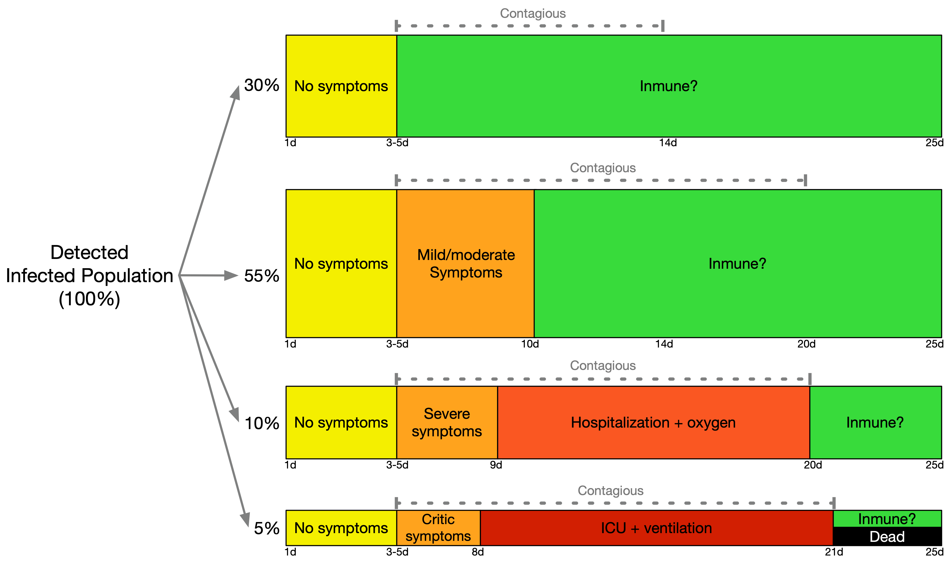
Before explaining in deeper details the extended transitions of our model, it is important to keep in mind that we have four kinds of infected people. While the asymptomatic and mild symptoms, and respectively, do not require hospitalization before recovering (and thus only contribute to the transmission dynamics), infected with severe and critical symptoms, and respectively, require hospitalization with different treatment. Infected with severe symptoms require intensive care and possibly the use of oxigen, and infected with critical symptoms will require ventilator treatment. Since the treatment of severe patients is limited by the number of hospitalization UCI beds, and the treatment of critical patients is limited by the number of ventilators, we consider a maximal (but time dependent) UCI-hospitalization (hospitalization from now on) and ventilator capacities and , respectively. Whenever the number of patients requiring each of this treatments reach its maximal capacity, the new infected people coming cannot receive the respective treatment and eventually die. Considering that the death rate is and with and without treatment capacity, it is extremely important understand the conditions under which such capacity is reached.
In order to facilitate the understanding of the situation we provide two figures. In the fig. 1 we show a diagram of the time and proportions of the different transitions compiling various sources in the literature [7, 2, 8, 23, 22, 24, 25], and in fig. 2 we show a compartmental-model-diagram of those transitions, making more explicit the way in which the differential equations are built.
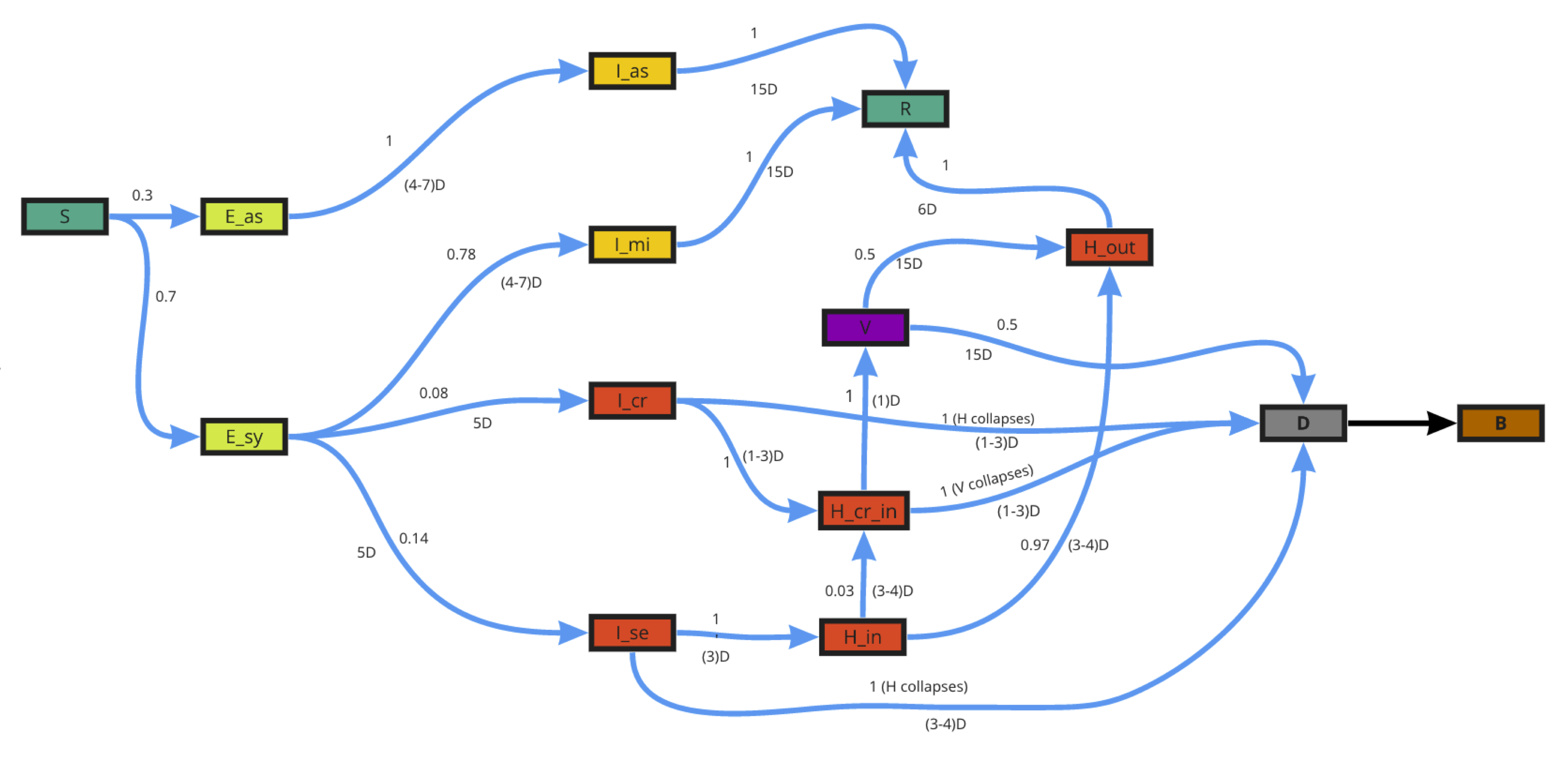
We will explain in more detail the transitions of the model in fig. 2:
-
•
Every susceptible can become exposed with an asymptomatic or symptomatic future. We introduce two exposed states and to differentiate them.
-
•
Every becomes infected asymptomatic , which later becomes recovered .
-
•
Every can become either infected with mild symptoms , infected with severe symptoms or infected with critical symptoms . While will not require hospitalization, will require basic hospitalization to recover (at most oxigen), and will require the use of a ventilator to recover.
-
•
Since not only the proportion but also the mobility of and is small compared to and , we consider that the infection rate depends only on and .
-
•
When is hospitalized, then it enters in a state which means it is hospitalized. From such state it can evolve to either meaning it will recover, or to meaning its symptoms worsen so it requires ventilation treatment.
-
•
If the hospitalization capacity is reached, then cannot be hospitalized and dies.
-
•
When is hospitalized it enters in state and goes to the ventilator treatment state . From , it can either improve and transit to ending up as recovered , or die during the treatment.
-
•
If the hospitalization capacity is reached, then and cannot be hospitalized (represented by states and respectively), and eventually transit to a dead state.
-
•
For both and those whose symptoms worsen, once hospitalized in state , if the ventilator capacity is reached, then they cannot enter in the ventilator treatment and die.
The system is ruled by the following equations
| (6) |
where the transition parameters represent the rate of the transition111the ratio between numbers above and below the arrow representing the transition in fig. 2. from state to state , is a function whose value is if and else, and is a function whose value is if and else.
The code for solving and analyze these equations is available for download in [26]. The parameter table is below
| rate | value | meaning |
|---|---|---|
| 0.19 | success of transmission infected to susceptible | |
| change from exposed to infected asymptomatic | ||
| change from exposed to infected mild symptoms | ||
| change from exposed to infected severe symptoms | ||
| change from exposed to infected critical symptoms | ||
| change from infected asymptomatic to recovered | ||
| change from infected asymptomatic to recovered | ||
| change from infected severe symptoms to hospitalized | ||
| change from infected critical symptoms to hospitalized | ||
| change from infected severe symptoms to death | ||
| change from infected critical symptoms to death | ||
| change from hospitalization state to start of the recovery | ||
| worsen of symptoms during hospitalization | ||
| change from hospitalization state to ventilation | ||
| change from hospitalization to death | ||
| change from ventilator to death | ||
| change from ventilator to start recovering | ||
| exit from hospitalization |
3 Preliminary Analysis
We will first study the interplay between the mobility function and the hospital capacities and using a numerical scenario.
We will concentrate in the SHFR defined by the ratio between the number of dead people by COVID19 and the number of infected people that require hospitalization.
| (7) |
From Fig. 1 we have that of the infected have either severe or critical symptoms, and in case there is no hospitalization capacity whatsoever they would all die. In this case . Moreover, since we have that the fraction of people with severe symptoms is twice the fraction of people with critical symptoms, we have that , and that the chance of recovering of hospitalized patients with severe symptoms is almost , while for the case of critical patients in ventilators, the chance of recovering is , we can estimate a lower bound of the as follows:
Hence, we have that in active pandemic conditions, i.e. if none of the measured variables are zero, should range between an optimal value and a worst value .
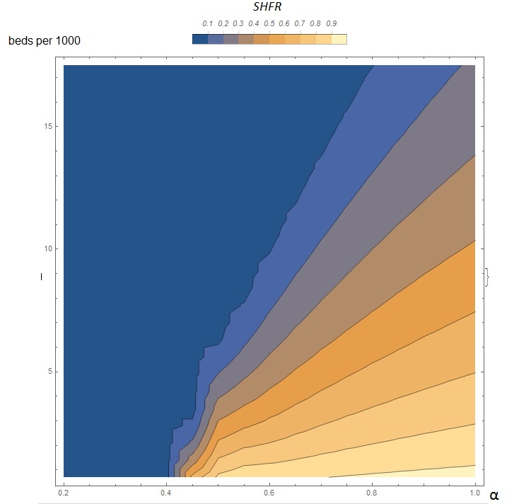
In our simulation we consider a system with people, and leave the parameter constant through each simulation at different values from to . Based on [27], we consider an estimate between 1 and 25 hospitalization beds per thousand people, covering most of the world’s realities, and estimate that . of such capacity corresponds to ventilators. This estimation can be considered rough, however, it is still useful for the purpose of understanding the interplay between hospitalization capacity and mobility.
In figure 3 we observe the converging SHFR value for the tested scenarios (convergence found to be stable after 250 days in all scenarios). It is interesting to note that in this case the mobility controls the pandemics in all possible scenarios. This result is consistent with [28] where a similar mobility parameter was found. This means that with mobility below there is no spread of the disease, i.e. . For we observe that in the absence of beds very little mobility induces a big increase in SHFR. For example in the bottom case (1 bed per thousand people), changing the mobility from to we increase SHFR from to , while the same change of mobility having 3 beds per thousand people increases SHFR up to .
It is well know from many mobility studies, such as the one developed by Google [9], that in the countries where measures to reduce the mobility have been implemented, the effective reductions range between and . Therefore, we must observe the interval . Clearly, in the case above 10 beds per thousand people the situation is under control with a minimal reduction of mobility. However, for the case below 5 beds per thousand people, results in SHFR greater than , implying that the severe patients have the same mortality than critical patients. Hence, the Infected Fatality Rate reaches the value of approximately.
4 Discussion
The mobility parameter is a way to introduce a reduction of the number of interactions from the baseline random mixing giving by . The mobility should be extended to incorporate the population density distribution, strong but specific deviations from average mobility, and the way people from different areas move to other areas.
In future work we will incorporate all these mobility aspects, and we consider important to incorporate the role that several other variables have in the system under study. For example, information technologies will have in the control of the disease by not only using AI to predict and detect trends, but also to incorporate tele-medicine to the possible treatments [29, 29]. Moreover, it is important to consider how other non-health related variables are impacted by the pandemics such as economical drops [30] and social demands.
5 Conclusion
We conclude that mobility must remain below to to control the pandemics without a hospitalization system, and when there is a hospitalization system the mobility can increase above , but only up to a limit which is specified by the number of beds available, as shown in Fig. 3. Using this model it is possible to provide a much deeper understanding of how to control the pandemics by forecasting the pandemic situation including both the reductions of mobility of different partial or total lockdowns and the plan for increase of hospital capacity which most countries are applying.
6 Acknowledgments
The authors acknowledge the access to supercomputing capacity from the National Laboratory for High Performance Computing (NLHPC), Universidad de Chile, Powered@NLHPC. Partial economic support is acknowledged to Programa de Apoyo a Centros con Financiamiento Basal AFB 170004 to FCV, Instituto Milenio Centro Interdisciplinario de Neurociencia de Valparaíso (ICM-ANID P09-022-F). Research was partially sponsored by the Army Research Laboratory under Cooperative Agreement Number W911NF-19-2-0242, and by the Air Force Office of Scientific Research under award number FA9550-19-1-0368. The views and conclusions contained in this document are those of the authors and should not be interpreted as representing the official policies, either expressed or implied, of the Army Research Laboratory or the U.S. Government. The U.S. Government is authorized to reproduce and distribute reprints for Government purposes notwithstanding any copyright notation herein. Any opinions, finding, and conclusions or recommendations expressed in this material are those of the author(s) and do not necessarily reflect the views of the United States Air Force.
References
- [1] S. Eubank, I. Eckstrand, B. Lewis, S. Venkatramanan, M. Marathe, and C. L. Barrett, “Commentary on ferguson, et al., "impact of non-pharmaceutical interventions (npis) to reduce covid-19 mortality and healthcare demand",” Bull Math Biol, vol. 82, p. 52, 04 2020.
- [2] S. A. Lauer, K. H. Grantz, Q. Bi, F. K. Jones, Q. Zheng, H. R. Meredith, A. S. Azman, N. G. Reich, and J. Lessler, “The incubation period of coronavirus disease 2019 (covid-19) from publicly reported confirmed cases: estimation and application,” Annals of internal medicine, vol. 172, no. 9, pp. 577–582, 2020.
- [3] L. Matrajt and T. Leung, “Evaluating the effectiveness of social distancing interventions to delay or flatten the epidemic curve of coronavirus disease.,” Emerging infectious diseases, vol. 26, no. 8, 2020.
- [4] F. E. Alvarez, D. Argente, and F. Lippi, “A simple planning problem for covid-19 lockdown,” tech. rep., National Bureau of Economic Research, 2020.
- [5] P. Walker, C. Whittaker, O. Watson, M. Baguelin, K. Ainslie, S. Bhatia, S. Bhatt, A. Boonyasiri, O. Boyd, L. Cattarino, et al., “Report 12: The global impact of covid-19 and strategies for mitigation and suppression,” 2020.
- [6] S. Das, P. Ghosh, B. Sen, and I. Mukhopadhyay, “Critical community size for covid-19–a model based approach to provide a rationale behind the lockdown,” arXiv preprint arXiv:2004.03126, 2020.
- [7] R. Verity, L. C. Okell, I. Dorigatti, P. Winskill, C. Whittaker, N. Imai, G. Cuomo-Dannenburg, H. Thompson, P. G. Walker, H. Fu, et al., “Estimates of the severity of coronavirus disease 2019: a model-based analysis,” The Lancet infectious diseases, 2020.
- [8] Y. Liu, L.-M. Yan, L. Wan, T.-X. Xiang, A. Le, J.-M. Liu, M. Peiris, L. L. Poon, and W. Zhang, “Viral dynamics in mild and severe cases of covid-19,” The Lancet Infectious Diseases, 2020.
- [9] Google, Local mobility report, 2020.
- [10] S. A. Al-Sheikh, “Modeling and analysis of an seir epidemic model with a limited resource for treatment,” Global Journal of Science Frontier Research Mathematics and Decision Sciences, vol. 12, no. 14, pp. 56–66, 2012.
- [11] W. Lyra, J. D. do Nascimento, J. Belkhiria, L. de Almeida, P. P. Chrispim, and I. de Andrade, “Covid-19 pandemics modeling with seir (+ caqh), social distancing, and age stratification. the effect of vertical confinement and release in brazil.,” medRxiv, 2020.
- [12] W. C. Roda, M. B. Varughese, D. Han, and M. Y. Li, “Why is it difficult to accurately predict the covid-19 epidemic?,” Infectious Disease Modelling, 2020.
- [13] N. Picchiotti, M. Salvioli, E. Zanardini, and F. Missale, “Covid-19 pandemic: a mobility-dependent seir model with undetected cases in italy, europe and us,” arXiv preprint arXiv:2005.08882, 2020.
- [14] K. Linka, M. Peirlinck, F. Sahli Costabal, and E. Kuhl, “Outbreak dynamics of covid-19 in europe and the effect of travel restrictions,” Computer Methods in Biomechanics and Biomedical Engineering, pp. 1–8, 2020.
- [15] L. López and X. Rodo, “A modified seir model to predict the covid-19 outbreak in spain and italy: simulating control scenarios and multi-scale epidemics,” Available at SSRN 3576802, 2020.
- [16] A. Chandak, D. Dey, B. Mukhoty, and P. Kar, “Epidemiologically and socio-economically optimal policies via bayesian optimization,” arXiv preprint arXiv:2005.11257, 2020.
- [17] N. Askitas, K. Tatsiramos, B. Verheyden, et al., “Lockdown strategies, mobility patterns and covid-19,” tech. rep., Institute of Labor Economics (IZA), 2020.
- [18] A. Pan, L. Liu, C. Wang, H. Guo, X. Hao, Q. Wang, J. Huang, N. He, H. Yu, X. Lin, et al., “Association of public health interventions with the epidemiology of the covid-19 outbreak in wuhan, china,” Jama, 2020.
- [19] Y. Fang, Y. Nie, and M. Penny, “Transmission dynamics of the covid-19 outbreak and effectiveness of government interventions: A data-driven analysis,” Journal of medical virology, vol. 92, no. 6, pp. 645–659, 2020.
- [20] C. Hou, J. Chen, Y. Zhou, L. Hua, J. Yuan, S. He, Y. Guo, S. Zhang, Q. Jia, C. Zhao, et al., “The effectiveness of quarantine of wuhan city against the corona virus disease 2019 (covid-19): A well-mixed seir model analysis,” Journal of medical virology, 2020.
- [21] D. W. Berger, K. F. Herkenhoff, and S. Mongey, “An seir infectious disease model with testing and conditional quarantine,” tech. rep., National Bureau of Economic Research, 2020.
- [22] M. Park, A. R. Cook, J. T. Lim, Y. Sun, and B. L. Dickens, “A systematic review of covid-19 epidemiology based on current evidence,” Journal of Clinical Medicine, vol. 9, no. 4, p. 967, 2020.
- [23] N. M. Ferguson, D. Laydon, G. Nedjati-Gilani, N. Imai, K. Ainslie, M. Baguelin, S. Bhatia, A. Boonyasiri, Z. Cucunubá, G. Cuomo-Dannenburg, et al., “Impact of non-pharmaceutical interventions (npis) to reduce covid-19 mortality and healthcare demand. 2020,” DOI, vol. 10, p. 77482, 2020.
- [24] G. Giordano, F. Blanchini, R. Bruno, P. Colaneri, A. Di Filippo, A. Di Matteo, and M. Colaneri, “Modelling the covid-19 epidemic and implementation of population-wide interventions in italy,” Nature Medicine, pp. 1–6, 2020.
- [25] G. E. Weissman, A. Crane-Droesch, C. Chivers, T. Luong, A. Hanish, M. Z. Levy, J. Lubken, M. Becker, M. E. Draugelis, G. L. Anesi, et al., “Locally informed simulation to predict hospital capacity needs during the covid-19 pandemic,” Annals of internal medicine, 2020.
- [26] Dlab, COVID19 Geomodeller project Github, 2020.
- [27] C. S. M. Barrientos, IndexMundi, 2020.
- [28] H. Xiong and H. Yan, “Simulating the infected population and spread trend of 2019-ncov under different policy by eir model,” Available at SSRN 3537083, 2020.
- [29] Z. Yang, Z. Zeng, K. Wang, S.-S. Wong, W. Liang, M. Zanin, P. Liu, X. Cao, Z. Gao, Z. Mai, et al., “Modified seir and ai prediction of the epidemics trend of covid-19 in china under public health interventions,” Journal of Thoracic Disease, vol. 12, no. 3, p. 165, 2020.
- [30] A. A. Toda, “Susceptible-infected-recovered (sir) dynamics of covid-19 and economic impact,” arXiv preprint arXiv:2003.11221, 2020.