MeshWalker: Deep Mesh Understanding by Random Walks

Abstract.

Most attempts to represent 3D shapes for deep learning have focused on volumetric grids, multi-view images and point clouds. In this paper we look at the most popular representation of 3D shapes in computer graphics—a triangular mesh—and ask how it can be utilized within deep learning. The few attempts to answer this question propose to adapt convolutions & pooling to suit Convolutional Neural Networks (CNNs). This paper proposes a very different approach, termed MeshWalker to learn the shape directly from a given mesh. The key idea is to represent the mesh by random walks along the surface, which ”explore” the mesh’s geometry and topology. Each walk is organized as a list of vertices, which in some manner imposes regularity on the mesh. The walk is fed into a Recurrent Neural Network (RNN) that ”remembers” the history of the walk. We show that our approach achieves state-of-the-art results for two fundamental shape analysis tasks: shape classification and semantic segmentation. Furthermore, even a very small number of examples suffices for learning. This is highly important, since large datasets of meshes are difficult to acquire.

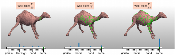
Figure 1. Classification by MeshWalker. This figure shows classification results as the walk (in green) proceeds along the surface of a camel ($4K$ faces) from SHREC11 (Lian et al., 2011). The initial point was randomly chosen on the neck. After $V/50$ steps (left), $V$ being the number of vertices, the system is uncertain regarding the class, and the highest probability predictions are for the flamingo class and for the hand class (out of $30$ classes). After continuing the random walk along the body and the front leg for $V/7$ steps, the probability of being a horse is higher than before, but the camel already has quite a high probability. Finally, after $V/2.5$ steps (right) and walking also along the hump, the system correctly classifies the model as a camel.

1. Introduction

The most-commonly used representation of surfaces in computer graphics is a polygonal mesh, due to its numerous benefits, including efficiency and high-quality. Nevertheless, in the era of deep learning, this representation is often bypassed because of its irregularity, which does not suit Convolutional Neural Networks (CNNs). Instead, 3D data is often represented as volumetric grids (Maturana and Scherer, 2015; Sedaghat et al., 2016b; Roynard et al., 2018; Ben-Shabat et al., 2018) or multiple 2D projections (Su et al., 2015; Boulch et al., 2017; Feng et al., 2018a; Yavartanoo et al., 2018; Kanezaki et al., 2018). In some recent works point clouds are utilized and new ways to convolve or pool are proposed (Atzmon et al., 2018; Xu et al., 2018; Li et al., 2018; Hua et al., 2018; Thomas et al., 2019).

Despite the benefits of these representations, they miss the notions of neighborhoods and connectivity and might not be as good for capturing local surface properties. Recently, several works have proposed to maintain the potential of the mesh representation, while still utilizing neural networks. FeaStNet (Verma et al., 2018) proposes a graph neural network in which the neighborhood of each vertex for the convolution operation is calculated dynamically based on its features. MeshCNN (Hanocka et al., 2019) defines pooling and convolution layers over the mesh edges. MeshNet (Feng et al., 2019) treats the faces of a mesh as the basic unit and extracts their spatial and structural features individually to offer the final semantic representation. LRF-Conv (Yang et al., 2020) learns descriptors directly from the raw mesh by defining new continuous convolution kernels that provide robustness to sampling. All these methods redefine the convolution operation, and by doing so, are able to fit the unordered structure of a mesh to a CNN framework.

We propose a novel and fundamentally different approach, named MeshWalker. As in previous approaches that learn directly from the mesh data, the basic question is how to impose regularity on the unordered data. Our key idea is to represent the mesh by random walks on its surface. These walks explore the local geometry of the surface, as well as its global one. Every walk is fed into a Recurrent Neural Network (RNN), that ”remembers” the walk’s history.

In addition to simplicity, our approach has three important benefits. First, we will show that even a small dataset suffices for training. Intuitively, we can generate multiple random walks for a single model; these walks provide multiple explorations of the model. This may be considered as equivalent to using different projections of 3D objects in the case of image datasets. Second, as opposed to CNNs, RNNs are inherently robust to sequence length. This is vital in the case of meshes, as datasets include objects of various granularities. Third, the meshes need not be watertight or have a single connected component; our approach can handle any triangular mesh.

Our approach is general and can be utilized to address a variety of shape analysis tasks. We demonstrate its benefit in two basic applications: mesh classification and mesh semantic segmentation. Our results are superior to those of state-of-the-art approaches on common datasets and on highly non-uniform meshes. Furthermore, when the training set is limited in size, the accuracy improvement over the state-of-the-art methods is highly evident.

Hence, this paper makes three contributions:

1. We propose a novel representation of meshes for neural networks: random walks on surfaces.

2. We present an end-to-end learning framework that realizes this representation within RNNs. We show that this framework works well even when the dataset is very small. This is important in the case of 3D, where large datasets are seldom available and are difficult to generate.

3. We demonstrate the benefits of our method in two key applications: 3D shape classification and semantic segmentation.

2. Related Work

Our work is at the crossroads of three fields, as discussed below.

2.1. Representing 3D objects for Deep Neural Networks

A variety of representations of 3D shapes have been proposed in the context of deep learning. The main challenge is how to re-organize the shape description such that it could be processed within deep learning frameworks. Hereafter we briefly review the main representations; see (Gezawa et al., 2020) for a recent excellent survey.

Multi-view 2D projections.

This representation is essentially a set of 2D images, each of which is a rendering of the object from a different viewpoint (Su et al., 2015; Kalogerakis et al., 2017; Qi et al., 2016; Sarkar et al., 2018; Gomez-Donoso et al., 2017; Johns et al., 2016; Zanuttigh and Minto, 2017; Bai et al., 2016; Wang et al., 2019c; Kanezaki et al., 2018; Feng et al., 2018b; He et al., 2018; Han et al., 2019). The major benefit of this representation is that it can naturally utilize any image-based CNN. In addition, high-resolution inputs can be easily handled. However, it is not easy to determine the optimal number of views; if that number is large, the computation might be costly. Furthermore, self-occlusions might be a drawback.

Volumetric grids.

These grids are analogous to the 2D grids of images. Therefore, the main benefit of this representation is that operations that are applied on 2D grids can be extended to 3D in a straightforward manner (Wu et al., 2015; Brock et al., 2016; Tchapmi et al., 2017; Fanelli et al., 2011; Maturana and Scherer, 2015; Wang et al., 2019a; Sedaghat et al., 2016a; Zhi et al., 2018). The primary drawbacks of volumetric grids are their limited resolution and the heavy computation cost needed.

Point clouds.

This representation consists of a set of 3D points, sampled from the object’s surface. The simplicity, close relationship to data acquisition, and the ease of conversion from other representations, make point clouds an attractive representation. Therefore, a variety of recent works proposed successful techniques for point cloud shape analysis using neural networks (Qi et al., 2017a, b; Wang et al., 2019d; Guerrero et al., 2018; Williams et al., 2019; Atzmon et al., 2018; Li et al., 2018; Liu et al., 2019; Xu et al., 2019; Zhu et al., 2019). These methods attempt to learn a representation for each point, using its neighbors (Euclidean-wise) either by multi layer perceptions or by convolutional layers. Some also define novel pooling layers. Point cloud representations might fall short in applications when the connectivity is highly meaningful (e.g. segmentation) or when the salient information is concentrated in small specific areas.

Triangular meshes.

This representation is the most widespread representation in computer graphics and the focus of our paper. The major challenge of using meshes within deep learning frameworks is the irregularity of the representation—each vertex has a different number of neighbors, at different distances.

The pioneering work of (Masci et al., 2015) introduces deep learning of local features and shows how to make the convolution operations intrinsic to the mesh. In (Poulenard and Ovsjanikov, 2018) a new convolutional layer is defined, which allows the propagation of geodesic information throughout the network layers. FeaStNet (Verma et al., 2018) proposes a graph neural network in which the neighborhood of each vertex for the convolution operation is calculated dynamically based on its features. Another line of works exploits the fact that local patches are approximately Euclidean. The 3D manifolds are then parameterized in 2D, where standard CNNs are utilized (Henaff et al., 2015; Sinha et al., 2016; Boscaini et al., 2016; Maron et al., 2017; Ezuz et al., 2017; Haim et al., 2019). A different approach is to apply a linear map to a spiral of neighbors (Gong et al., 2019; Lim et al., 2018), which works well for meshes with a similar graph structure.

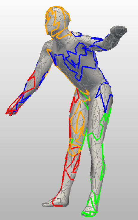
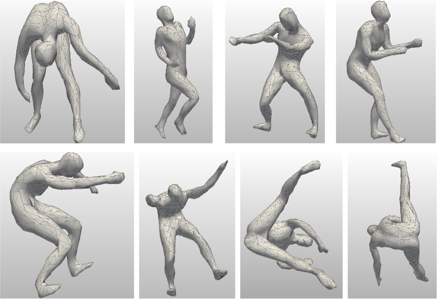
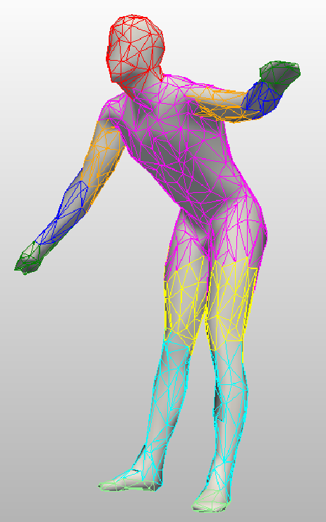
(a) $5$ walks on the surface	(b) Classification: Samples from the class the input belongs to	(c) Semantic segmentation

Figure 2. Outline. To explore a mesh, walks on its surface are generated and study the surface both locally and globally (a). These walks provide sufficient information to perform shape analysis tasks, such as classification and segmentation. Specifically, (b) shows samples from the class to which MeshWalker correctly classified the model from (a) and (c) shows the resulting segmentation. The models are from SHREC11 (Lian et al., 2011).

Two approaches were recently introduced: MeshNet (Feng et al., 2019) treats faces of a mesh as the basic unit and extracts their spatial and structural features individually, to offer the final semantic representation. MeshCNN (Hanocka et al., 2019) is based on a very unique idea of using the edges of the mesh to perform pooling and convolution. The convolution operations exploit the regularity of edges—having $4$ edges of their incidental triangles. An edge collapse operation is used for pooling, which maintains surface topology and generates new mesh connectivity for further convolutions.

2.2. Classification

Object classification refers to the task of classifying a given shape into one of pre-defined categories. Before deep learning methods became widespread, the main challenges were finding good descriptors and good distance functions between these descriptors. According to the thorough review of (Lian et al., 2013), the methods could be roughly classified into algorithms employing local features (Johnson and Hebert, 1999; Lowe, 2004; Liu et al., 2006; Sun et al., 2009; Ovsjanikov et al., 2009), topological structures (Hilaga et al., 2001; Sundar et al., 2003; Tam and Lau, 2007), isometry-invariant global geometric properties (Reuter et al., 2005; Jain and Zhang, 2007; Mahmoudi and Sapiro, 2009), direct shape matching, or canonical forms (Mémoli and Sapiro, 2005; Mémoli, 2007; Bronstein et al., 2006; Elad and Kimmel, 2003).

Many of the recent techniques already use deep learning for classification. They are described in Section 2.1, for instance (Hanocka et al., 2018; Qi et al., 2017a, b; Li et al., 2018; Ezuz et al., 2017; Bronstein et al., 2011; Feng et al., 2019; Thomas et al., 2019; Liu et al., 2019; Veličković et al., 2017; Wang et al., 2019b; Kipf and Welling, 2016; Perozzi et al., 2014).

2.3. Semantic segmentation

Mesh segmentation is a key ingredient in many computer graphics tasks, including modeling, animation and a variety of shape analysis tasks. The goal is to determine, for the basic elements of the mesh (vertex, edge or face), to which segment they belong. Many approaches were proposed, including region growing (Chazelle et al., 1997; Lavoué et al., 2005; Zhou and Huang, 2004; Koschan, 2003; Sun et al., 2002; Katz et al., 2005), clustering (Shlafman et al., 2002; Katz and Tal, 2003; Gelfand and Guibas, 2004; Attene et al., 2006), spectral analysis (Alpert and Yao, 1995; Gotsman, 2003; Liu and Zhang, 2004; Zhang et al., 2005) and more. See (Attene et al., 2006; Shamir, 2008; Rodrigues et al., 2018) for excellent surveys of segmentation methods.

Lately, deep learning has been utilized for this task as well. Each proposed approach handles a specific shape representation, as described in Section 2.1. These approaches include among others  (Hanocka et al., 2018; Qi et al., 2017a, b; Li et al., 2018; Yang et al., 2020; Haim et al., 2019; Maron et al., 2017; Qi et al., 2017b; Guo et al., 2015).

3. MeshWalker outline

Imagine an ant walking on a surface; it will ”climb” on ridges and go through valleys. Thus, it will explore the local geometry of the surface, as well as the global terrain. Random walks have been shown to incorporate both global and local information about a given object (Lai et al., 2008; Lovász et al., 1993; Grady, 2006; Noh and Rieger, 2004). This information may be invaluable for shape analysis tasks, nevertheless, random walks have not been used to represent meshes within a deep learning framework before.

Given a polygonal mesh, we propose to randomly walk through the vertices of the mesh, along its edges, as shown in Fig. 2(a). In our ant analogy, the longer the walk, the more information is acquired by the ant. But how shall this information be accumulated? We propose to feed this representation into a Recurrent Neural Network (RNN) framework, which aggregates properties of the walk. This aggregated information will enable the ant to perceive the shape of the mesh. This is particularly beneficial for shape analysis tasks that require both the 3D global structure and some local information of the mesh, as demonstrated in Fig. 2(b-c).

Algorithm 1 describes the training procedure of our proposed MeshWalker approach. A defining property of it is that the same piece of algorithm is used for every vertex along the walk (i.e., each vertex the ant passes through). The algorithm iterates on the following: A mesh is first extracted from the dataset (it could be a mesh that was previously extracted). A vertex is chosen randomly as the head of the walk and then a random walk is generated. This walk is the input to an RNN model. Finally, the RNN model’s parameters $\theta$ are updated by minimizing the Softmax cross entropy loss $L$, using Adam optimizer (Kingma and Ba, 2014).

Input: Labeled mesh dataset, $\mathcal{M}$

Output: $\theta$—RNN model parameters

$\theta_{0}\leftarrow RNN$ random parameters;

$\mathcal{M}\leftarrow$ MeshPreprocessing($\mathcal{M}$);

repeat

      $(M_{i},y_{i})\leftarrow$ random mesh $M_{i}\in\mathcal{M}$ and label(s) $y_{i}$;

      $v_{ij}\leftarrow$ random starting vertex;

      ${w_{ij}\leftarrow GenerateWalk(M_{i},v_{ij})}$;

      ${x}_{ij}\leftarrow RepresentWalk(M_{i},w_{ij})$;

      $\theta_{i}\leftarrow learningFromWalks(\theta_{i-1},{x}_{ij},y_{i})$;

     

      until Convergence;

ALGORITHM 1 MeshWalker Training

Section 4 elaborates on the architecture of our MeshWalker learning model, as well as on each of the ingredients of the iterative step. Section 6.2 explains the mesh pre-processing step, which essentially performs mesh simplification, and provides implementation details.

4. Learning to walk over a surface

This section explains how to realize Algorithm 1. It begins by elaborating on the construction of a random walk on a mesh. It then proceeds to describe the network that learns from walks in order to understand meshes.

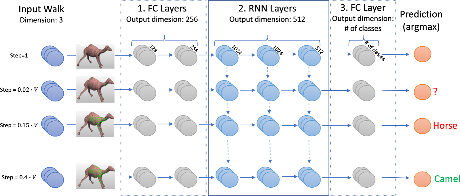
Figure 3. Network architecture. The network consists of three components: The first component (FC layers) changes the feature space; the second component (RNN layers) aggregates the information along the walk; and the third component (an FC layer) predicts the outcome of the network. For classification, the prediction of the last vertex of the walk is considered and Softmax is applied to its resulting vector (the bottom-right orange circle, classified as a camel). For segmentation (not shown in this figure), the network is similar. However, Softmax is applied to each of the resulting vectors of the vertices (the orange circles in the right column); each vertex is classified into a segment.

4.1. What is a walk?

Walks provide a novel way to organize the mesh data. A walk is a sequence of vertices (not necessarily adjacent), each of which is associated with basic information.

Walk generation.

We adopt a very simple strategy to generate walks, out of many possible ones. Recall that we are given the first vertex $v_{ij}$ of a walk. Then, to generate the walk $w_{ij}$, the other vertices are iteratively added, as follows. Given the current vertex of the walk, the next vertex is chosen randomly from its adjacent vertices (those that belong to its one-ring neighbors).

If such a vertex does not exist (as all the neighbors already belong to the walk), the walk is tracked backwards until an un-visited neighbor is found; this neighbor is added to the walk. In this case, the walk is not a linear sequence of vertices connected via edges, but rather a tree. If the mesh consists of multiple connected component, it is possible that the walk reaches a dead-end. In this case, a new random un-visited vertex is chosen and the walk generation proceeds as before. We note that in all cases, the input to the RNN is a sequence of vertices, arranged by their discovery order. In practice, the length of the walk is set by default to $\lceil V/2.5\rceil$, where $V$ is number of vertices.

Walk representation.

Once the walk $w_{ij}$ is determined, the representation $x_{ij}$ of this walk should be defined; this would be the input to the RNN. Each vertex is represented as the 3D translation from the previous vertex in the walk (${\Delta X,\Delta Y,\Delta Z}$). This is inline with the deep learning philosophy, which prefers end-to-end learning instead of hand-crafted features that are separated from a classifier, We note that we also tried other representations, including vertex coordinates, normals, and curvatures, but the results did not improve.

Walks at inference time.

At inference, several walks are being used for each mesh. Each walk produces a vector of probabilities to belong to the different classes (in the case of classification). These vectors are averaged to produce the final result. To understand the importance of averaging, let us consider the walks on the camel in Fig. 1. Since walks are generated randomly, we expect some of them to explore atypical parts of the model, such as the legs, which are similar to horse legs. Other walks, however, are likely to explore unique parts, such as the hump or the head. The average result will most likely be the camel, as will be shown in Section 5.

4.2. Learning from walks

Once walks are defined, the next challenge is to distillate the information accumulated along a walk into a single descriptor vector. Hereafter we discuss the network architecture and the training.

Network architecture.

The model consists of three sub-networks, as illustrated in Fig. 3. The first sub-network is given the current vertex of the walk and learns a new feature space, i.e. it transforms the 3D input feature space into a 256D feature space. This is done by two fully connected (FC) layers, followed by an instance normalization (Ulyanov et al., 2016) layer and ReLu as nonlinear activation; both empirically outperform other alternatives.

The second sub-network is the core of our approach. It utilizes a recurrent neural network (RNN) whose defining property is being able to ”remember” and accumulate knowledge. Briefly, a recurrent neural network (Graves et al., 2008; Hochreiter and Schmidhuber, 1997; Cho et al., 2014) is a connectionist model that contains a self-connected hidden layer. The benefit of self-connection is that the ‘memory’ of previous inputs remains in the network’s internal state, allowing it to make use of past context. In our setting, the RNN gets as input a feature vector (the result of the previous sub-network), learns the hidden states that describe the walk up to the current vertex, and outputs a state vector that contains the information gathered along the walk.

Another benefit of RNNs, which is crucial in our case, is not being confined to fixed-length inputs or outputs. Thus, we can use the model to inference on a walk of a certain length, which may differ from walk lengths the model was trained on.

To implement the RNN part of our model, we use three Gated Recurrent Unit (GRU) layers of (Cho et al., 2014). Briefly, the goal of an GRU layer is to accumulate only the important information from the input sequence and to forget the non-important information.

Formally, let $x_{t}$ be the input at time $t$ and $h_{t}$ be the hidden state at time $t$; let the reset gate $r_{t}$ and the update gate $z_{t}$ be two vectors, which jointly decide which information should be passed from time $t$-$1$ to time $t$. To realize GRU’s goal, the network performs the following calculation, which sets the hidden state at time $t$. Its final content is based on updating the hidden state in the previous time (the update gate $z_{t}$ determines which information should be passed) and on its candidate memory content $\tilde{h}_{t}$:

(1) $$h_{t}=z_{t}\odot h_{t-1}+\left(1-z_{t}\right)\odot\tilde{h}_{t},$$

where $\odot$ is an element-wise multiplication. Here, $\tilde{h}_{t}$ is defined as:

(2) $$\tilde{h}_{t}=\tanh\left(W^{(h)}x_{t}+U^{(h)}h_{t-1}\odot r_{t}+b^{(h)}\right).$$

That is, when the reset gate is close to $0$, the hidden state ignores the previous hidden state and resets with the current input only. This effectively allows the hidden state to drop any information that will later be found to be irrelevant.

Finally, the reset gate $r_{t}$ and the update gate $z_{t}$ are defined as:

(3) $$z_{t}=\sigma\left(W^{(z)}x_{t}+U^{(z)}h_{t-1}+b^{(z)}\right),$$

(4) $$r_{t}=\sigma\left(W^{(r)}x_{t}+U^{(r)}h_{t-1}+b^{(r)}\right),$$

where $\sigma$ is a logistic Sigmoid function. $W^{(h)},W^{(z)},W^{(r)},U^{(h)},U^{(z)}$ and $U^{(r)}$ are trainable weight matrices and $b^{(h)},b^{(r)},b^{(r)}$ are trainable bias vectors. The initial hidden state $h_{j}$ is set to $0$.

GRU outperforms a vanilla RNN, due to its ability to both remember the important information along the sequence and to forget unimportant content. Furthermore, it is capable of processing long sequences, similarly to the Long Short-Term Memory (LSTM) (Hochreiter and Schmidhuber, 1997). Being able to accumulate information from long sequences is vital for grasping the shape of a 3D model, which usually consists of thousands of vertices. We chose GRU over LSTM due to its simplicity and its smaller computational requirements. For comparison, LSTM would require $16.8M$ trainable parameters in our case, whereas $GRU$ uses $12.7M$. Furthermore, the inference time is smaller—for instance, a single $100$-steps walk takes $5mSec$ using LSTM and $3mSec$ using GRU.

The third sub-network in Fig. 3 predicts the object class in case of classification, or the vertex segment in case of semantic segmentation. It consists of a single fully connected (FC) layer on top of the state vector calculated in the previous sub-network. More details on the architectures & the implementation are given in Section 6.

Loss calculation.

The Softmax cross entropy loss is used on the output of the third part of the network. In the case of the classification task, only the last step of the walk is used as input to the loss function, since it accumulates all prior information from the walk. In Fig. 3, this is the bottom-right orange component.

In the case of the segmentation task, each vertex has its own predicted segment class. Each of the orange components in Fig. 3 classifies the segment that the respected vertex belongs to. Since at the beginning of the walk the results are not trustworthy (as the mesh is not yet well understood), for the loss calculation in the training process we consider the segment class predictions only for the vertices that belong to the second half of the walk.

5. Applications: Classification & Segmentation

MeshWalker is a general approach, which may be applied to a variety of applications. We demonstrate its performance for two fundamental tasks in shape analysis: mesh classification and mesh semantic segmentation. Our results are compared against the reported SOTA results for recently-used datasets, hence the methods we compare against vary according to the specific dataset.

5.1. Mesh classification

Given a mesh, the goal is to classify it into one of pre-defined classes. For the given mesh we generate multiple random walks. These walks are run through the trained network. For each walk, the network predicts the probability of this mesh to belong to each class. These prediction vectors are averaged into a single prediction vector. In practice we use $32$ walks; Section 6 will discuss the robustness of MeshWalker to the number of walks.

To test our algorithm, we applied our method to three recently-used datasets: SHREC11 (Lian et al., 2011), engraved cubes  (Hanocka et al., 2019) and ModelNet40 (Wu et al., 2015), which differ from each other in the number of classes, the number of objects per class, as well as the type of shapes they contain. As common, the accuracy is defined as the ratio of correctly predicted meshes.

SHREC11.

This dataset consists of $30$ classes, with 20 examples per class. Typical classes are camels, cats, glasses, centaurs, hands etc. Following the setup of (Ezuz et al., 2017), we split the objects in each class into $16$ (/$10$) training examples and $4$ (/$10$) testing examples.

Table 1 compares the performance, where each result is the average of the results of $3$ randoms splits (of $16/4$ or of $10/10$). When the split is $10$ objects for training and $10$ for testing, the advantage of our method is apparent. When $16$ objects are used for training and only $4$ for testing, we get the same accuracy as that of the current state-of-the-art. In Section 6.1 we show that indeed the smaller the training dataset, the more advantageous our approach is.

Table 1. Classification on SHREC11 (Lian et al., 2011). Split-$16$ and Split-$10$ are the number of training models per class (out of $20$ models in the class). In both cases our method achieves state-of-the-art results, yet it is most advantageous for a small training dataset (Split-$10$). (We have not found point cloud-based networks that were tested on SHREC11).

Method	Input	Split-$1$6	Split-$10$
MeshWalker (ours)	Mesh	98.6%	97.1%
MeshCNN (Hanocka et al., 2019)	Mesh	98.6%	91.0%
GWCNN (Ezuz et al., 2017)	Mesh	96.6%	90.3%
SG (Bronstein et al., 2011)	Mesh	70.8%	62.6%

Cube engraving.

This dataset contains $4600$ objects, with $3910$/$690$ training/testing split. Each object is a cube ”engraved” with a shape at a random face in a random location, as demonstrated in Fig. 4. The engraved shape belongs to a dataset of $23$ classes (e.g., car, heart, apple, etc.), each contains roughly $20$ shapes. This dataset was created in order to demonstrate that using meshes, rather than point clouds, may be critical for 3D shape analysis.

Table 2 provides the results. It demonstrates the benefit of our method over state-of-the-art methods.

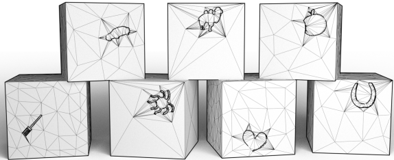
Figure 4. Engraved cubes dataset. This image is courtesy of (Hanocka et al., 2019).

Table 2. Classification on Cube Engraving (Hanocka et al., 2019). Our results outperform those of state-of-the-art algorithms.

Method	Input	accuracy
MeshWalker (ours)	Mesh	98.6%
MeshCNN (Hanocka et al., 2019)	Mesh	92.16%
PointNet++ (Qi et al., 2017b)	Point cloud	64.26%

ModelNet40.

This commonly-used dataset contains $12,311$ CAD models from $40$ categories, out of which $9,843$ models are used for training and $2,468$ models are used for testing. Unlike previous datasets, many of the objects contain multiple components and are not necessarily watertight, making this dataset prohibitive for some mesh-based methods. However, such models can be handled by MeshWalker since as explained before, if the walk gets into a dead-end during backtracking, it jumps to a new random location.

Table 3 shows that our results outperform those of mesh-based state-of-the-art methods. We note that without $5$ classes that are cross-labeled (desk/table & plant/flower-pot/vase) our method’s accuracy is $94.4\%$. The table shows that multi-views approaches are excellent for this dataset. This is due to relying on networks that are pre-trained on a large number of images. However, they might fail for other datasets, such as the engraved cubes, and do not suit other shape analysis tasks, such as semantic segmentation.

Table 3. Classification on ModelNet40 (Wu et al., 2015). MeshWalker is competitive with other mesh-based methods. Multi-view methods are advantageous for this dataset, possibly due to relying on pre-trained networks for image classification and to naturally handling multiple components and non–watertight models, which characterize many meshes in this dataset.

Method	Input	Accuracy
MeshWalker (ours)	mesh	92.3%
MeshNet (Feng et al., 2019)	mesh	91.9%
SNGC (Haim et al., 2019)	mesh	91.6%
KPConv (Thomas et al., 2019)	point cloud	92.9%
PointNet (Qi et al., 2017a)	point cloud	89.2%
RS-CNN (Liu et al., 2019)	point cloud	93.6%
RotationNet (Kanezaki et al., 2018)	multi-views	97.3%
GVCNN (Feng et al., 2018b)	multi-views	93.1%
3D2SeqViews (Han et al., 2019)	multi-views	93.4%

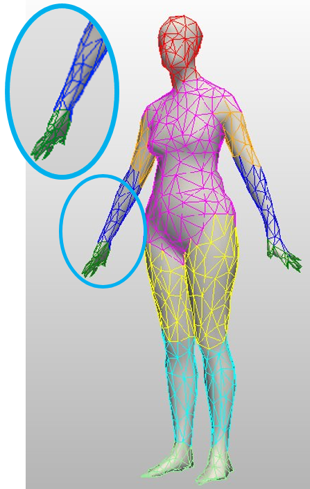
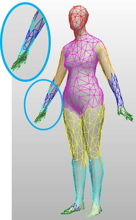
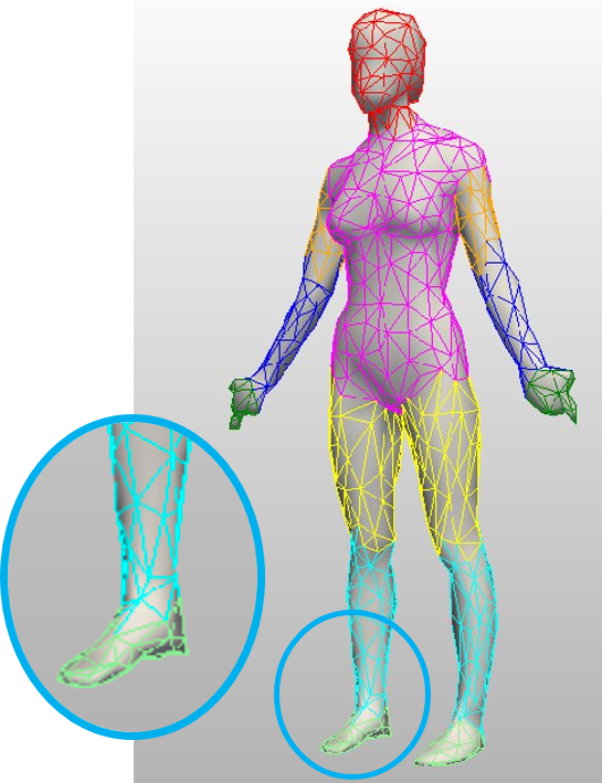
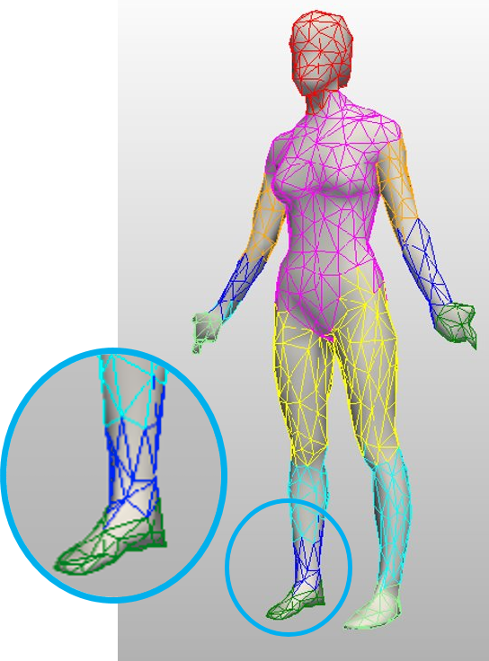
(a) Ours	(b) (Hanocka et al., 2019)	(c) Ours	(d) (Hanocka et al., 2019)

Figure 5. Qualitative results for human shape segmentation from (Maron et al., 2017). Our system avoids mis-classifications, not mixing lower legs with lower arms or hands with feet. We note that for most shapes in the dataset, both systems produce equally-good results.

5.2. Mesh semantic segmentation

Shape segmentation is an important building block for many applications in shape analysis and synthesis. The goal is to determine, for every vertex, the segment it belongs to. We tested MeshWalker on two datasets: COSEG (Wang et al., 2012) and human-body Segmentation (Maron et al., 2017).

Given mesh, multiple random walks are generated (in practice, $32$ $\times$ # segment classes; see the discussion in Section 6). These walks are run through the trained network, which predicts the probabilities of belonging to the segments. Similarly to the training process, only vertices of the second half of each walk are considered trustworthy. For each vertex, the predictions of the walks it belongs to are averaged. Then, as post-processing, we consider the average prediction of the vertex neighbors and add this average with $0.5$ weight. Finally, the prediction for each vertex is the argmax-ed.

Formally, let $\{W\}$ be the set of walks performed on a mesh. Let $P^{i}_{v}$ be the vector that is the Softmax output for vertex $v$ from walk $i$ (if walk $i$ does not visit $v$, $P^{i}_{v}$ is set to a $0$-vector). Let $v^{ring}$ be the list of the vertices adjacent to $v$ and $N_{v}$ be the size of this list. The predicted label, $l_{v}$ of vertex $v$ is defined as (where $argmax$ finds the maximum vector entry):

(5) $$l_{v}=argmax(\sum_{i\in\{W\}}P^{i}_{v}+\frac{1}{2N_{v}}\sum_{\tilde{v}\in v^{ring}}\sum_{i\in\{W\}}P^{i}_{{\tilde{v}}}).$$

We follow the accuracy measure proposed in (Hanocka et al., 2019): Given the prediction for each edge, the accuracy is defined as the percentage of the correctly-labeled edges, weighted by their length. Since MeshWalker predicts the segment of the vertices, if the predictions of the endpoints of the edge agree, the edge gets the endpoints’ label; otherwise, the label with the higher prediction is chosen. The overall accuracy is the average over all meshes.

Human-body segmentation.

The dataset consists of $370$ training models from SCAPE (Anguelov et al., 2005), FAUST (Bogo et al., 2014), MIT (Vlasic et al., 2008) and Adobe Fuse (Adobe, 2016). The test set consists of $18$ humans from SHREC’07 (Giorgi et al., 2007) . The meshes are manually segmented into eight labeled segments according to (Kalogerakis et al., 2010).

Table 4. Human-body segmentation results on (Maron et al., 2017). The accuracy is calculated on edges of the simplified meshes.

Method	Edge Accuracy
MeshWalker	94.8%
MeshCNN	92.3%

Table 5. Human-body segmentation results on (Maron et al., 2017). The reported results are on the original meshes; For MeshCNN, the results shown are ours. Our results outperform those of state-of-the-art algorithms.

Method	Input	Face
		Accuracy
MeshWalker (ours)	Mesh	92.7%
MeshCNN (Hanocka et al., 2019)	Mesh	89.0%
LRF-Conv (Yang et al., 2020)	Mesh	89.9%
SNGC (Haim et al., 2019)	Mesh	91.3%
Toric Cover (Maron et al., 2017)	Mesh	88.0%
GCNN (Masci et al., 2015)	Mesh	86.4%
MDGCNN	Mesh	89.5%
(Poulenard and Ovsjanikov, 2018)
PointNet++ (Qi et al., 2017b)	Point cloud	90.8%
DynGraphCNN (Wang et al., 2019d)	Point cloud	89.7%

There are two common measures of segmentation results, according to the correct classification of faces (Haim et al., 2019) or of edges (Hanocka et al., 2019). Tables 4 and 5 compare our results to those of previous works, according to the reported measure and the type of objects (simplified or not). Since our method is trained on simplified meshes, to get results on the original meshes, we apply a simple projection to the original meshes jointly with boundary smoothing, as in (Katz and Tal, 2003). In both measures, MeshWalker outperforms other methods. Fig. 5 presents qualitative examples where the difference between the resulting segmentations is evident.

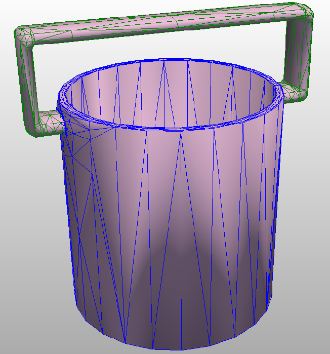
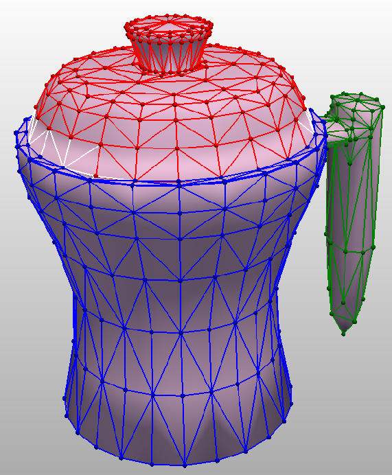
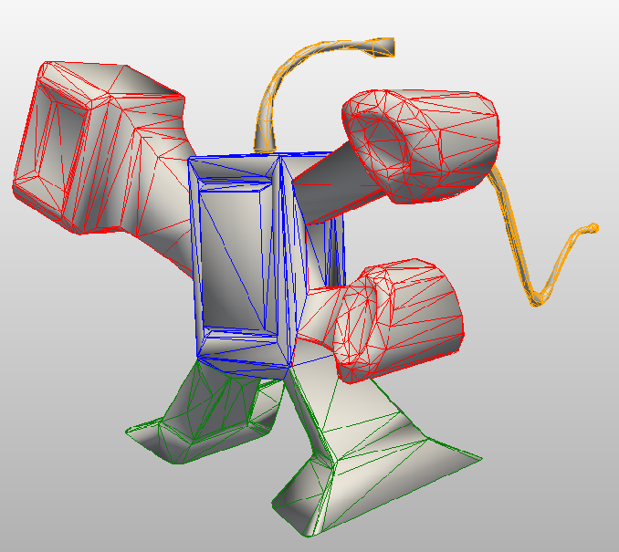
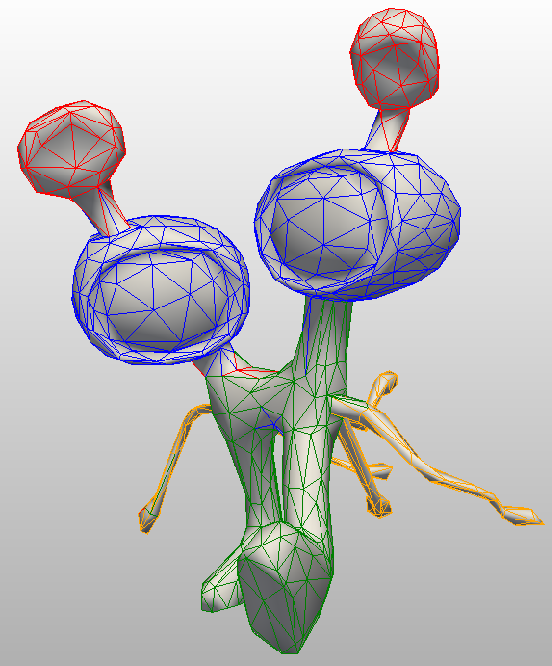
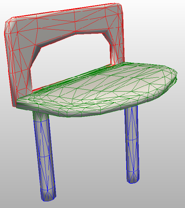
(a) Vases	(b) Aliens	(c) Chairs

Figure 6. Qualitative results of segmentation for meshes from COSEG (Wang et al., 2012).

COSEG segmentation.

This dataset contains three large classes: aliens, vases and chairs with $200$, $300$ and $400$ shapes, respectively. Each category is split into $85\%$/$15\%$ train/test sets. Fig. 6 presents some qualitative results, where it can be seen that our method performs very well. Table 6 shows the accuracy of our results, where the results of the competitors are reported in (Hanocka et al., 2019). Our method achieves state-of-the-art results for all categories.

Table 6. Segmentation results on COSEG (Wang et al., 2012). Our method achieves state-of-the-art results for all categories.

Method	Vases	Chairs	Telealiens	Mean
MeshWalker (ours)	98.7%	99.6%	99.1%	99.1%
MeshCNN	97.3%	99.6%	97.6%	98.2%
PointNet++	94.7%	98.9%	79.1%	90.9%
PointCNN (Li et al., 2018)	96.4%	99.3%	97.4%	97.7%

6. Experiments

6.1. Ablation study

Size of the training dataset.

How many training models are needed in order to achieve good performance? In the 3D case this question is especially important, since creating a dataset is costly. Table 7 shows the accuracy of our model for the COSEG dataset, when trained on different dataset sizes. As expected, the larger the dataset, the better the results. However, even when using only $4$ shapes for training, the results are pretty good ($80.5\%$). This outstanding result can be explained by the fact that we can produce many random walks for each mesh, hence the actual number of training examples is large. This result is consistent across all categories and datasets. Table 8 shows a similar result for the human-body segmentation dataset.

Table 7. Analysis of the training dataset size (COSEG segmentation). ”Full” training is $170$, $255$ and $240$ shapes for tele-aliens, vases and chairs, respectively. As expected, the larger the dataset, the better the results. However, even if the training dataset is very small, our results are good.

# training shapes	Vases	Chairs	Tele-aliens	Mean
Full	$98.7\%$	$99.6\%$	$99.1\%$	$99.1\%$
32	$95.3\%$	$98.5\%$	$94.2\%$	$96.0\%$
16	$93.6\%$	$93.4\%$	$92.4\%$	$93.1\%$
8	$83.7\%$	$87.7\%$	$86.7\%$	$86.0\%$
4	$77.5\%$	$83.7\%$	$80.4\%$	$80.5\%$
2	$67.3\%$	$78.4\%$	$69.7\%$	$71.8\%$
1	$60.9\%$	$59.9\%$	$40.6\%$	$53.8\%$

Table 8. Analysis of the training dataset size (human-body segmentation). As before, the performance of our method degrades gracefully with the size of the training set. We note that the results of MeshCNN are not reported in their paper, but rather the results of new runs of their system.

# training shapes	MeshWalker	MeshCNN
	(ours)	(Hanocka et al., 2019)
381 (full)	94.8%	$92.3\%$
16	92.0%	$55.7\%$
4	84.3%	$48.3\%$
2	80.8%	$42.4\%$

Walk length.

Fig. 1 has shown that the accuracy of our method depends on the walk length. What would be an ideal length for our system to ”understand” a shape? Fig. 7 analyzes the influence of the length on the task of classification for SHREC11. As expected, the accuracy increases with length. However, it can be seen that when we use at least $16$ walks per mesh, a walk whose length is $0.15V$ suffices to get excellent results. Furthermore, there is a trade-off between the number of walks we use and the length of these walks. Though the exact length depends both on the task in hand and on the dataset, this correlation is consistent across datasets and tasks.

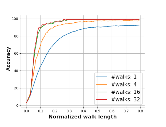
Figure 7. Walk length analysis. The accuracy increases with walk length, for classification on SHREC11. Here, the $X$ axis is number of vertices along the walk, normalized by number of mesh vertices. This figure illustrates trade-off between the number of walks we use and the length of these walks. As the walk begins, using many walks is not beneficial since the RNN has not accumulated enough information yet. However, after e.g. 0.3V, two walks are better than a single 0.6V-length walk. This is because they explore different mesh regions.

Number of walks.

How many walks are needed at inference time? Table 9 shows that the more walks, the better the accuracy. However, even very few walks result in very good accuracy. In particular, on SHREC11, even with a single walk the accuracy is $90.8\%$. For the Engraved-Cubes dataset, more walks are needed, since the model is engraved on a single cube facet, which certain walks might not get to. Even in this difficult case, $4$ walks already achieve $92.1\%$ accuracy. We note that the STD is between $2.5\%$ for a single walk to $0.4\%$ for $32$ walks. As expected, the more walks used, the more stable the results are and the smaller the STD is.

Table 9. Number of walks analysis. The accuracy improves with the number of walks per shape (demonstrated on $2$ datasets).

# Walks	SHREC11 Acc	Eng.Cubes Acc
$32$	$98.3\%$	$97.6$%
$16$	$97.8\%$	$97.4$%
$8$	$97.8\%$	$95.3$%
$4$	$95.5\%$	$92.1$%
$2$	$95.0\%$	$84.8$%
$1$	$90.8\%$	$77.1$%

Robustness.

We use various rotations within data augmentation, hence robustness to orientations. In particular, to test the robustness to rotation, we rotated the models in the Human-body segmentation dataset and in SHREC11 classification dataset $36$ times for each axis, by increments of $10^{\circ}$. For each of these rotated versions of the datasets we applied the same testing as before. For both datasets, there was no difference in the results. Furthermore, the meshes are normalized, hence robustness to scaling.

Our approach is inherently robust to different triangulations, as random walks (representing the same mesh) may vary greatly anyhow. Specifically, we generated a modified version of the COSEG segmentation dataset by randomly perturbing $30\%$ of the vertex positions, realized as a shift towards a random vertex in its $1$-ring. The performance degradation is less than $0.1\%$.

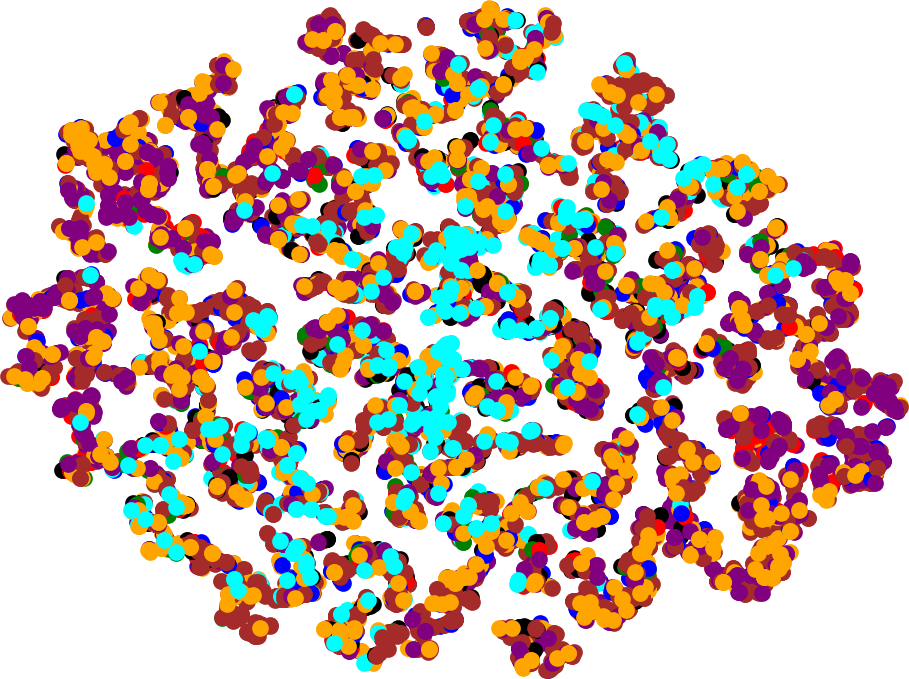
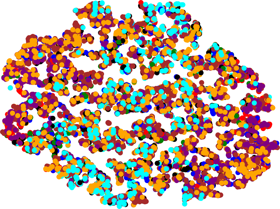
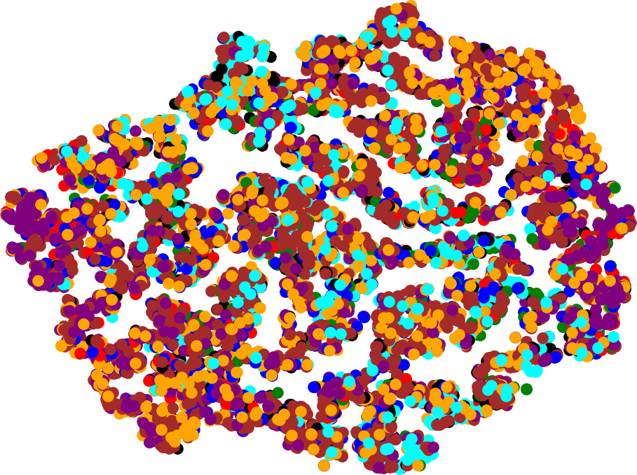
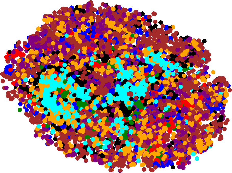
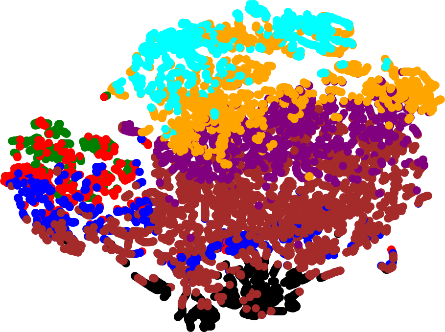
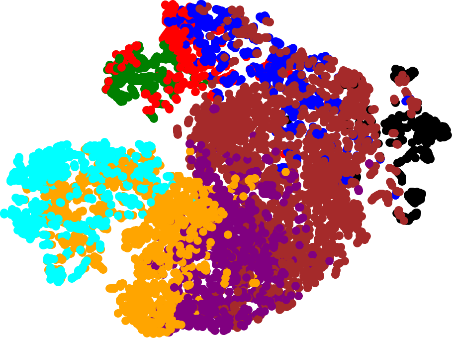
(a) input	(b) FC1	(c) FC2	(d) GRU1	(e) GRU2	(f) GRU3

Figure 8. t-SNE of the internal layers. This is a visualization of the output of the different layers for the human-body segmentation task. It can be seen how the semantic meaning of the layers’ output starts to evolve after the first GRU layer and gets better in the next two layers.

6.2. Implementation

Mesh pre-processing: simplification & data augmentation.

All the meshes used for training are first simplified into roughly the same number of faces (Garland and Heckbert, 1997; Hoppe, 1997) (MeshProcessing procedure in Algorithm 1). Simplification is analogous to the initial resizing of images. It reduces the network capacity required for training. Moreover, we could use several simplifications for each mesh as a form of data augmentation for training and for testing. For instance, for ModelNet40 we use $1K$, $2K$ and $4K$ faces. The meshes are normalized into a unit sphere, if necessary.

In addition, we augment the training data and add diversity by rotating the models. As part of batch preparation, each model is randomly rotated in each axis prior to each training iteration.

t-SNE analysis.

Does the network produce meaningful features? Fig. 8 opens the network’s ”black box” and shows the t-SNE projection to 2D of the multi-dimensional features after each stage of our learning framework, applied to the human-body segmentation task. Each feature vector is colored by its correct label.

In the input layer all the classes are mixed together. The same behavior is noticed after the first two fully-connected layers, since no information is shared between the vertices up to this stage. In the next three GRU layers, semantic meaning evolves: The features are structured as we get deeper in the network. In the last RNN layer the features are meaningful, as the clusters are evident. This visualization demonstrates the importance of the RNN hierarchy.

Fig. 9 reveals another invaluable property of our walks. It shows the t-SNE visualization of walks for classification of objects from $5$ categories of SHREC11. Each feature vector is colored by its correct label; its shape (rectangle, triangle etc) represents the object the walk belongs to. Not only clusters of shapes from the same category clearly emerge, but also walks that belong to the same object are grouped together! This is another indication to the quality of our proposed features.

Computation time.

Training takes between $5$ hours (for classification on SHREC11) to $12$ hours (for segmentation on human-body), using GTX 1080 TI graphics card. At inference, a $100$-step walk, which is typical for SHREC11, takes about $4$ milliseconds. When we use $32$ walks per shape, the running time would be $128$ milliseconds. Remeshing takes e.g. $4.6$ seconds from $400K$ faces to $1.5K$ or $0.85$ from $100K$ face to $1.5K$ faces. We note that our method is easy to parallelize, as every walk could be processed on a different processor, which is yet another benefit of our approach.

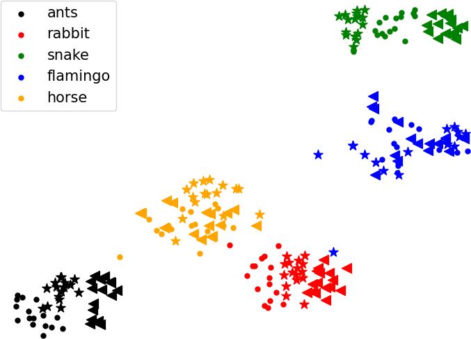
Figure 9. t-SNE analysis for classification. This figure shows feature hierarchy: Meshes that belong to the same category (indicated by the color) are clustered together. Furthermore, walks that belong to the same mesh (indicated by the shape of the 2D point) are also clustered.

Training configurations.

We implemented our network using TensorFlow V2. The network architecture is given in Table 10. The source code is available on "https://github.com/AlonLahav/MeshWalker".

Table 10. Training configuration

Layer	Output Dimension
Vertex description	$3$
Fully Connected	$128$
Instance Normalization	$128$
ReLU	$128$
Fully Connected	$256$
Instance Normalization	$256$
ReLU	$256$
GRU	$1024$
GRU	$1024$
GRU	$512$
Fully Connected	# of classes

Optimization: To update the network weights, we use Adam optimizer (Kingma and Ba, 2014). The learning rate is set in a cyclic way, as suggested by (Smith, 2017). The initial and the maximum learning rates are set to $10^{-6}$ and $5\cdot 10^{-4}$ respectively. The cycle size is $20k$ iterations.

Batch strategy: Walks are grouped into batches of $32$ walks each. For mesh classification, the walks are generated from different meshes, whereas for semantic segmentation each batch is composed of $4$ walks on $8$ meshes.

Training iterations: We train for $60$k, $60$k, $460$k, $200$k, $200$k iterations for SHREC11, COSEG, human-body segmentation, engraved-cubes and ModelNet40 datasets, respectively. This is so since for the loss to converge fast, many of the walks should cover the salient parts of the shape, which distinguish it from other classes/segments. When this is not the case, more iterations are needed in order for the few meaningful walks to influence the loss. This is the case for instance in the engraved cubes dataset, where the salient information lies on a single facet.

6.3. Limitations

Fig. 10 shows a failure of our algorithm, where parts of the hair were wrongly classified as a torso. This is the case since the training data does not contain enough models with hair to learn from. In general, learning-based algorithms rely on good training data, which is not always available.

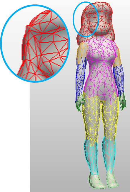
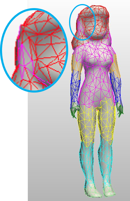
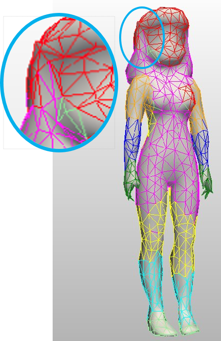
(a) Ground truth	(b) Ours	(c) (Hanocka et al., 2019)

Figure 10. Limitation. Our algorithm fails to classify the hair due to not having sufficient similar shapes in the dataset.

Another limitation is handling large meshes. The latter require long walks, which in turn might lead to run-time and memory issues. In this paper, this is solved by simplifying the meshes and then projecting the segmentation results onto the original meshes. (For classification, this is not a concern, as simplified meshes may be used).

7. Conclusion

This paper has introduced a novel approach for representing meshes within deep learning schemes. The key idea is to represent the mesh by random walks on its surface, which intuitively explore the shape of the mesh. Since walks are described by the order of visiting mesh vertices, they suit deep learning.

Utilizing this representation, the paper has proposed an end-to-end learning framework, termed MeshWalker. The random walks are fed into a Recurrent Neural Network (RNN), that ”remembers” the walk’s history (i.e. the geometry of the mesh). Prior works indicated that RNNs are unsuitable for point clouds due to both the unordered nature of the data and the number of vertices used to represent a shape. Surprisingly, we have shown that RNNs work extremely well for meshes, through the concept of random walks.

Our approach is general, yet simple. It has several additional benefits. Most notably, it works well even for extremely small datasets. e.g. even $4$ meshes per class suffice to get good results. In addition, the meshes are not require to be watertight or to consist of a single component (as demonstrated by ModelNet40 (Wu et al., 2015)); some other mesh-based approaches impose these conditions and require the meshes to be manifolds.

Last but not least, the power of this approach has been demonstrated for two key tasks in shape analysis: mesh classification and mesh semantic segmentation. In both cases, we present state-of-the-art results.

An interesting question for future work is whether there are optimal walks for meshes, rather than random walks. For instance, are there good starting points of walks? Additionally, reinforcement learning could be utilized to learn good walks. Exploring other applications, such as shape correspondence, is another intriguing future direction. Another interesting practical future work would be to work on the mesh as is, without simplification as pre-processing.

- (1)
- Adobe (2016) Adobe. 2016. Adobe Fuse 3D Characters. https://www.mixamo.com.
- Alpert and Yao (1995) Charles J Alpert and So-Zen Yao. 1995. Spectral partitioning: the more eigenvectors, the better. In Proceedings of the 32nd annual ACM/IEEE Design Automation Conference. 195–200.
- Anguelov et al. (2005) Dragomir Anguelov, Praveen Srinivasan, Daphne Koller, Sebastian Thrun, Jim Rodgers, and James Davis. 2005. SCAPE: shape completion and animation of people. In ACM SIGGRAPH 2005 Papers. 408–416.
- Attene et al. (2006) Marco Attene, Bianca Falcidieno, and Michela Spagnuolo. 2006. Hierarchical mesh segmentation based on fitting primitives. The Visual Computer 22, 3 (2006), 181–193.
- Attene et al. (2006) M. Attene, S. Katz, M. Mortara, G. Patane, M. Spagnuolo, and A. Tal. 2006. Mesh Segmentation - A Comparative Study. In IEEE International Conference on Shape Modeling and Applications 2006 (SMI’06). 7–7.
- Atzmon et al. (2018) Matan Atzmon, Haggai Maron, and Yaron Lipman. 2018. Point convolutional neural networks by extension operators. arXiv preprint arXiv:1803.10091 (2018).
- Bai et al. (2016) Song Bai, Xiang Bai, Zhichao Zhou, Zhaoxiang Zhang, and Longin Jan Latecki. 2016. Gift: A real-time and scalable 3d shape search engine. In Proceedings of the IEEE conference on computer vision and pattern recognition. 5023–5032.
- Ben-Shabat et al. (2018) Yizhak Ben-Shabat, Michael Lindenbaum, and Anath Fischer. 2018. 3dmfv: Three-dimensional point cloud classification in real-time using convolutional neural networks. IEEE Robotics and Automation Letters 3, 4 (2018), 3145–3152.
- Bogo et al. (2014) Federica Bogo, Javier Romero, Matthew Loper, and Michael J Black. 2014. FAUST: Dataset and evaluation for 3D mesh registration. In Proceedings of the IEEE Conference on Computer Vision and Pattern Recognition. 3794–3801.
- Boscaini et al. (2016) Davide Boscaini, Jonathan Masci, Emanuele Rodolà, and Michael Bronstein. 2016. Learning shape correspondence with anisotropic convolutional neural networks. In Advances in neural information processing systems. 3189–3197.
- Boulch et al. (2017) Alexandre Boulch, Bertrand Le Saux, and Nicolas Audebert. 2017. Unstructured Point Cloud Semantic Labeling Using Deep Segmentation Networks. 3DOR 2 (2017), 7.
- Brock et al. (2016) Andrew Brock, Theodore Lim, James M Ritchie, and Nick Weston. 2016. Generative and discriminative voxel modeling with convolutional neural networks. arXiv preprint arXiv:1608.04236 (2016).
- Bronstein et al. (2011) Alexander M Bronstein, Michael M Bronstein, Leonidas J Guibas, and Maks Ovsjanikov. 2011. Shape google: Geometric words and expressions for invariant shape retrieval. ACM Transactions on Graphics (TOG) 30, 1 (2011), 1–20.
- Bronstein et al. (2006) Alexander M Bronstein, Michael M Bronstein, and Ron Kimmel. 2006. Efficient computation of isometry-invariant distances between surfaces. SIAM Journal on Scientific Computing 28, 5 (2006), 1812–1836.
- Chazelle et al. (1997) Bernard Chazelle, David P Dobkin, Nadia Shouraboura, and Ayellet Tal. 1997. Strategies for polyhedral surface decomposition: an experimental study. Computational Geometry 7, 5-6 (1997), 327–342.
- Cho et al. (2014) Kyunghyun Cho, Bart Van Merriënboer, Caglar Gulcehre, Dzmitry Bahdanau, Fethi Bougares, Holger Schwenk, and Yoshua Bengio. 2014. Learning phrase representations using RNN encoder-decoder for statistical machine translation. arXiv preprint arXiv:1406.1078 (2014).
- Elad and Kimmel (2003) Asi Elad and Ron Kimmel. 2003. On bending invariant signatures for surfaces. IEEE Transactions on pattern analysis and machine intelligence 25, 10 (2003), 1285–1295.
- Ezuz et al. (2017) Danielle Ezuz, Justin Solomon, Vladimir G Kim, and Mirela Ben-Chen. 2017. GWCNN: A metric alignment layer for deep shape analysis. In Computer Graphics Forum, Vol. 36. Wiley Online Library, 49–57.
- Fanelli et al. (2011) Gabriele Fanelli, Thibaut Weise, Juergen Gall, and Luc Van Gool. 2011. Real time head pose estimation from consumer depth cameras. In Joint pattern recognition symposium. Springer, 101–110.
- Feng et al. (2019) Yutong Feng, Yifan Feng, Haoxuan You, Xibin Zhao, and Yue Gao. 2019. MeshNet: mesh neural network for 3D shape representation. In Proceedings of the AAAI Conference on Artificial Intelligence, Vol. 33. 8279–8286.
- Feng et al. (2018a) Yifan Feng, Zizhao Zhang, Xibin Zhao, Rongrong Ji, and Yue Gao. 2018a. GVCNN: Group-View Convolutional Neural Networks for 3D Shape Recognition. In The IEEE Conference on Computer Vision and Pattern Recognition (CVPR).
- Feng et al. (2018b) Yifan Feng, Zizhao Zhang, Xibin Zhao, Rongrong Ji, and Yue Gao. 2018b. GVCNN: Group-view convolutional neural networks for 3D shape recognition. In Proceedings of the IEEE Conference on Computer Vision and Pattern Recognition. 264–272.
- Garland and Heckbert (1997) Michael Garland and Paul S Heckbert. 1997. Surface simplification using quadric error metrics. In Proceedings of the 24th annual conference on Computer graphics and interactive techniques. 209–216.
- Gelfand and Guibas (2004) Natasha Gelfand and Leonidas J Guibas. 2004. Shape segmentation using local slippage analysis. In Proceedings of the 2004 Eurographics/ACM SIGGRAPH symposium on Geometry processing. 214–223.
- Gezawa et al. (2020) Abubakar Sulaiman Gezawa, Yan Zhang, Qicong Wang, and Lei Yunqi. 2020. A Review on Deep Learning Approaches for 3D Data Representations in Retrieval and Classifications. IEEE Access 8 (2020), 57566–57593.
- Giorgi et al. (2007) Daniela Giorgi, Silvia Biasotti, and Laura Paraboschi. 2007. Shape retrieval contest 2007: Watertight models track. SHREC competition 8, 7 (2007).
- Gomez-Donoso et al. (2017) Francisco Gomez-Donoso, Alberto Garcia-Garcia, J Garcia-Rodriguez, Sergio Orts-Escolano, and Miguel Cazorla. 2017. Lonchanet: A sliced-based cnn architecture for real-time 3d object recognition. In 2017 International Joint Conference on Neural Networks (IJCNN). IEEE, 412–418.
- Gong et al. (2019) Shunwang Gong, Lei Chen, Michael Bronstein, and Stefanos Zafeiriou. 2019. Spiralnet++: A fast and highly efficient mesh convolution operator. In Proceedings of the IEEE International Conference on Computer Vision Workshops. 0–0.
- Gotsman (2003) Craig Gotsman. 2003. On graph partitioning, spectral analysis, and digital mesh processing. In 2003 Shape Modeling International. IEEE, 165–171.
- Grady (2006) Leo Grady. 2006. Random walks for image segmentation. IEEE transactions on pattern analysis and machine intelligence 28, 11 (2006), 1768–1783.
- Graves et al. (2008) Alex Graves, Marcus Liwicki, Santiago Fernández, Roman Bertolami, Horst Bunke, and Jürgen Schmidhuber. 2008. A novel connectionist system for unconstrained handwriting recognition. IEEE transactions on pattern analysis and machine intelligence 31, 5 (2008), 855–868.
- Guerrero et al. (2018) Paul Guerrero, Yanir Kleiman, Maks Ovsjanikov, and Niloy J Mitra. 2018. PCPNet learning local shape properties from raw point clouds. In Computer Graphics Forum, Vol. 37. Wiley Online Library, 75–85.
- Guo et al. (2015) Kan Guo, Dongqing Zou, and Xiaowu Chen. 2015. 3d mesh labeling via deep convolutional neural networks. ACM Transactions on Graphics (TOG) 35, 1 (2015), 1–12.
- Haim et al. (2019) Niv Haim, Nimrod Segol, Heli Ben-Hamu, Haggai Maron, and Yaron Lipman. 2019. Surface Networks via General Covers. In Proceedings of the IEEE International Conference on Computer Vision. 632–641.
- Han et al. (2019) Zhizhong Han, Honglei Lu, Zhenbao Liu, Chi-Man Vong, Yu-Shen Liu, Matthias Zwicker, Junwei Han, and CL Philip Chen. 2019. 3d2seqviews: Aggregating sequential views for 3d global feature learning by cnn with hierarchical attention aggregation. IEEE Transactions on Image Processing 28, 8 (2019), 3986–3999.
- Hanocka et al. (2018) Rana Hanocka, Noa Fish, Zhenhua Wang, Raja Giryes, Shachar Fleishman, and Daniel Cohen-Or. 2018. Alignet: Partial-shape agnostic alignment via unsupervised learning. ACM Transactions on Graphics (TOG) 38, 1 (2018), 1–14.
- Hanocka et al. (2019) Rana Hanocka, Amir Hertz, Noa Fish, Raja Giryes, Shachar Fleishman, and Daniel Cohen-Or. 2019. MeshCNN: a network with an edge. ACM Transactions on Graphics (TOG) 38, 4 (2019), 1–12.
- He et al. (2018) Xinwei He, Yang Zhou, Zhichao Zhou, Song Bai, and Xiang Bai. 2018. Triplet-center loss for multi-view 3d object retrieval. In Proceedings of the IEEE Conference on Computer Vision and Pattern Recognition. 1945–1954.
- Henaff et al. (2015) Mikael Henaff, Joan Bruna, and Yann LeCun. 2015. Deep convolutional networks on graph-structured data. arXiv preprint arXiv:1506.05163 (2015).
- Hilaga et al. (2001) Masaki Hilaga, Yoshihisa Shinagawa, Taku Kohmura, and Tosiyasu L Kunii. 2001. Topology matching for fully automatic similarity estimation of 3D shapes. In Proceedings of the 28th annual conference on Computer graphics and interactive techniques. 203–212.
- Hochreiter and Schmidhuber (1997) Sepp Hochreiter and Jürgen Schmidhuber. 1997. Long short-term memory. Neural computation 9, 8 (1997), 1735–1780.
- Hoppe (1997) Hugues Hoppe. 1997. View-dependent refinement of progressive meshes. In Proceedings of the 24th annual conference on Computer graphics and interactive techniques. 189–198.
- Hua et al. (2018) Binh-Son Hua, Minh-Khoi Tran, and Sai-Kit Yeung. 2018. Pointwise convolutional neural networks. In Proceedings of the IEEE Conference on Computer Vision and Pattern Recognition. 984–993.
- Jain and Zhang (2007) Varun Jain and Hao Zhang. 2007. A spectral approach to shape-based retrieval of articulated 3D models. Computer-Aided Design 39, 5 (2007), 398–407.
- Johns et al. (2016) Edward Johns, Stefan Leutenegger, and Andrew J Davison. 2016. Pairwise decomposition of image sequences for active multi-view recognition. In Proceedings of the IEEE Conference on Computer Vision and Pattern Recognition. 3813–3822.
- Johnson and Hebert (1999) Andrew E. Johnson and Martial Hebert. 1999. Using spin images for efficient object recognition in cluttered 3D scenes. IEEE Transactions on pattern analysis and machine intelligence 21, 5 (1999), 433–449.
- Kalogerakis et al. (2017) Evangelos Kalogerakis, Melinos Averkiou, Subhransu Maji, and Siddhartha Chaudhuri. 2017. 3D shape segmentation with projective convolutional networks. In Proceedings of the IEEE Conference on Computer Vision and Pattern Recognition. 3779–3788.
- Kalogerakis et al. (2010) Evangelos Kalogerakis, Aaron Hertzmann, and Karan Singh. 2010. Learning 3D mesh segmentation and labeling. In ACM SIGGRAPH 2010 papers. 1–12.
- Kanezaki et al. (2018) Asako Kanezaki, Yasuyuki Matsushita, and Yoshifumi Nishida. 2018. Rotationnet: Joint object categorization and pose estimation using multiviews from unsupervised viewpoints. In Proceedings of the IEEE Conference on Computer Vision and Pattern Recognition. 5010–5019.
- Katz et al. (2005) Sagi Katz, George Leifman, and Ayellet Tal. 2005. Mesh segmentation using feature point and core extraction. The Visual Computer 21, 8-10 (2005), 649–658.
- Katz and Tal (2003) Sagi Katz and Ayellet Tal. 2003. Hierarchical mesh decomposition using fuzzy clustering and cuts. ACM transactions on graphics (TOG) 22, 3 (2003), 954–961.
- Kingma and Ba (2014) Diederik P Kingma and Jimmy Ba. 2014. Adam: A method for stochastic optimization. arXiv preprint arXiv:1412.6980 (2014).
- Kipf and Welling (2016) Thomas N Kipf and Max Welling. 2016. Semi-supervised classification with graph convolutional networks. arXiv preprint arXiv:1609.02907 (2016).
- Koschan (2003) AF Koschan. 2003. Perception-based 3D triangle mesh segmentation using fast marching watersheds. In 2003 IEEE Computer Society Conference on Computer Vision and Pattern Recognition, 2003. Proceedings., Vol. 2. IEEE, II–II.
- Lai et al. (2008) Yu-Kun Lai, Shi-Min Hu, Ralph R. Martin, and Paul L. Rosin. 2008. Fast Mesh Segmentation Using Random Walks. In Proceedings of the 2008 ACM Symposium on Solid and Physical Modeling (SPM ’08). ACM, New York, NY, USA, 183–191. https://doi.org/10.1145/1364901.1364927
- Lavoué et al. (2005) Guillaume Lavoué, Florent Dupont, and Atilla Baskurt. 2005. A new CAD mesh segmentation method, based on curvature tensor analysis. Computer-Aided Design 37, 10 (2005), 975–987.
- Li et al. (2018) Yangyan Li, Rui Bu, Mingchao Sun, Wei Wu, Xinhan Di, and Baoquan Chen. 2018. Pointcnn: Convolution on x-transformed points. In Advances in neural information processing systems. 820–830.
- Lian et al. (2011) Z Lian, A Godil, B Bustos, M Daoudi, J Hermans, S Kawamura, Y Kurita, G Lavoua, and P Dp Suetens. 2011. Shape retrieval on non-rigid 3D watertight meshes. In Eurographics workshop on 3d object retrieval (3DOR). Citeseer.
- Lian et al. (2013) Zhouhui Lian, Afzal Godil, Benjamin Bustos, Mohamed Daoudi, Jeroen Hermans, Shun Kawamura, Yukinori Kurita, Guillaume Lavoué, Hien Van Nguyen, Ryutarou Ohbuchi, et al. 2013. A comparison of methods for non-rigid 3D shape retrieval. Pattern Recognition 46, 1 (2013), 449–461.
- Lim et al. (2018) Isaak Lim, Alexander Dielen, Marcel Campen, and Leif Kobbelt. 2018. A simple approach to intrinsic correspondence learning on unstructured 3d meshes. In Proceedings of the European Conference on Computer Vision (ECCV). 0–0.
- Liu and Zhang (2004) Rong Liu and Hao Zhang. 2004. Segmentation of 3D meshes through spectral clustering. In 12th Pacific Conference on Computer Graphics and Applications, 2004. PG 2004. Proceedings. IEEE, 298–305.
- Liu et al. (2019) Yongcheng Liu, Bin Fan, Shiming Xiang, and Chunhong Pan. 2019. Relation-shape convolutional neural network for point cloud analysis. In Proceedings of the IEEE Conference on Computer Vision and Pattern Recognition. 8895–8904.
- Liu et al. (2006) Yi Liu, Hongbin Zha, and Hong Qin. 2006. Shape topics: A compact representation and new algorithms for 3d partial shape retrieval. In 2006 IEEE Computer Society Conference on Computer Vision and Pattern Recognition (CVPR’06), Vol. 2. IEEE, 2025–2032.
- Lovász et al. (1993) László Lovász et al. 1993. Random walks on graphs: A survey. Combinatorics, Paul erdos is eighty 2, 1 (1993), 1–46.
- Lowe (2004) David G Lowe. 2004. Distinctive image features from scale-invariant keypoints. International journal of computer vision 60, 2 (2004), 91–110.
- Mahmoudi and Sapiro (2009) Mona Mahmoudi and Guillermo Sapiro. 2009. Three-dimensional point cloud recognition via distributions of geometric distances. Graphical Models 71, 1 (2009), 22–31.
- Maron et al. (2017) Haggai Maron, Meirav Galun, Noam Aigerman, Miri Trope, Nadav Dym, Ersin Yumer, Vladimir G Kim, and Yaron Lipman. 2017. Convolutional neural networks on surfaces via seamless toric covers. ACM Trans. Graph. 36, 4 (2017), 71–1.
- Masci et al. (2015) Jonathan Masci, Davide Boscaini, Michael Bronstein, and Pierre Vandergheynst. 2015. Geodesic convolutional neural networks on riemannian manifolds. In Proceedings of the IEEE international conference on computer vision workshops. 37–45.
- Maturana and Scherer (2015) Daniel Maturana and Sebastian Scherer. 2015. Voxnet: A 3d convolutional neural network for real-time object recognition. In 2015 IEEE/RSJ International Conference on Intelligent Robots and Systems (IROS). IEEE, 922–928.
- Mémoli (2007) Facundo Mémoli. 2007. On the use of Gromov-Hausdorff distances for shape comparison. (2007).
- Mémoli and Sapiro (2005) Facundo Mémoli and Guillermo Sapiro. 2005. A theoretical and computational framework for isometry invariant recognition of point cloud data. Foundations of Computational Mathematics 5, 3 (2005), 313–347.
- Noh and Rieger (2004) Jae Dong Noh and Heiko Rieger. 2004. Random walks on complex networks. Physical review letters 92, 11 (2004), 118701.
- Ovsjanikov et al. (2009) Maks Ovsjanikov, Alexander M Bronstein, Michael M Bronstein, and Leonidas J Guibas. 2009. Shape google: a computer vision approach to isometry invariant shape retrieval. In 2009 IEEE 12th International Conference on Computer Vision Workshops, ICCV Workshops. IEEE, 320–327.
- Perozzi et al. (2014) Bryan Perozzi, Rami Al-Rfou, and Steven Skiena. 2014. Deepwalk: Online learning of social representations. In Proceedings of the 20th ACM SIGKDD international conference on Knowledge discovery and data mining. 701–710.
- Poulenard and Ovsjanikov (2018) Adrien Poulenard and Maks Ovsjanikov. 2018. Multi-directional geodesic neural networks via equivariant convolution. ACM Transactions on Graphics (TOG) 37, 6 (2018), 1–14.
- Qi et al. (2017a) Charles R Qi, Hao Su, Kaichun Mo, and Leonidas J Guibas. 2017a. Pointnet: Deep learning on point sets for 3d classification and segmentation. In Proceedings of the IEEE conference on computer vision and pattern recognition. 652–660.
- Qi et al. (2016) Charles R Qi, Hao Su, Matthias Nießner, Angela Dai, Mengyuan Yan, and Leonidas J Guibas. 2016. Volumetric and multi-view cnns for object classification on 3d data. In Proceedings of the IEEE conference on computer vision and pattern recognition. 5648–5656.
- Qi et al. (2017b) Charles Ruizhongtai Qi, Li Yi, Hao Su, and Leonidas J Guibas. 2017b. Pointnet++: Deep hierarchical feature learning on point sets in a metric space. In Advances in neural information processing systems. 5099–5108.
- Reuter et al. (2005) Martin Reuter, Franz-Erich Wolter, and Niklas Peinecke. 2005. Laplace-spectra as fingerprints for shape matching. In Proceedings of the 2005 ACM symposium on Solid and physical modeling. 101–106.
- Rodrigues et al. (2018) Rui SV Rodrigues, José FM Morgado, and Abel JP Gomes. 2018. Part-based mesh segmentation: a survey. In Computer Graphics Forum, Vol. 37. Wiley Online Library, 235–274.
- Roynard et al. (2018) Xavier Roynard, Jean-Emmanuel Deschaud, and François Goulette. 2018. Classification of point cloud scenes with multiscale voxel deep network. arXiv preprint arXiv:1804.03583 (2018).
- Sarkar et al. (2018) Kripasindhu Sarkar, Basavaraj Hampiholi, Kiran Varanasi, and Didier Stricker. 2018. Learning 3d shapes as multi-layered height-maps using 2d convolutional networks. In Proceedings of the European Conference on Computer Vision (ECCV). 71–86.
- Sedaghat et al. (2016a) Nima Sedaghat, Mohammadreza Zolfaghari, Ehsan Amiri, and Thomas Brox. 2016a. Orientation-boosted voxel nets for 3d object recognition. arXiv preprint arXiv:1604.03351 (2016).
- Sedaghat et al. (2016b) Nima Sedaghat, Mohammadreza Zolfaghari, and Thomas Brox. 2016b. Orientation-boosted Voxel Nets for 3D Object Recognition. CoRR abs/1604.03351 (2016). arXiv:1604.03351 http://arxiv.org/abs/1604.03351
- Shamir (2008) Ariel Shamir. 2008. A survey on mesh segmentation techniques. In Computer graphics forum, Vol. 27. Wiley Online Library, 1539–1556.
- Shlafman et al. (2002) Shymon Shlafman, Ayellet Tal, and Sagi Katz. 2002. Metamorphosis of polyhedral surfaces using decomposition. In Computer graphics forum, Vol. 21. Wiley Online Library, 219–228.
- Sinha et al. (2016) Ayan Sinha, Jing Bai, and Karthik Ramani. 2016. Deep learning 3D shape surfaces using geometry images. In European Conference on Computer Vision. Springer, 223–240.
- Smith (2017) Leslie N Smith. 2017. Cyclical learning rates for training neural networks. In 2017 IEEE Winter Conference on Applications of Computer Vision (WACV). IEEE, 464–472.
- Su et al. (2015) Hang Su, Subhransu Maji, Evangelos Kalogerakis, and Erik Learned-Miller. 2015. Multi-view convolutional neural networks for 3d shape recognition. In Proceedings of the IEEE international conference on computer vision. 945–953.
- Sun et al. (2009) Jian Sun, Maks Ovsjanikov, and Leonidas Guibas. 2009. A concise and provably informative multi-scale signature based on heat diffusion. In Computer graphics forum, Vol. 28. Wiley Online Library, 1383–1392.
- Sun et al. (2002) Yiyong Sun, David Lon Page, Joon Ki Paik, Andreas Koschan, and Mongi A Abidi. 2002. Triangle mesh-based edge detection and its application to surface segmentation and adaptive surface smoothing. In Proceedings. International Conference on Image Processing, Vol. 3. IEEE, 825–828.
- Sundar et al. (2003) Hari Sundar, Deborah Silver, Nikhil Gagvani, and Sven Dickinson. 2003. Skeleton based shape matching and retrieval. In 2003 Shape Modeling International. IEEE, 130–139.
- Tam and Lau (2007) G Tam and R Lau. 2007. Deformable model retrieval based on topological and geometric signatures. IEEE transactions on visualization and computer graphics. 13, 3 (2007), 470–482.
- Tchapmi et al. (2017) Lyne Tchapmi, Christopher Choy, Iro Armeni, JunYoung Gwak, and Silvio Savarese. 2017. Segcloud: Semantic segmentation of 3d point clouds. In 2017 international conference on 3D vision (3DV). IEEE, 537–547.
- Thomas et al. (2019) Hugues Thomas, Charles R Qi, Jean-Emmanuel Deschaud, Beatriz Marcotegui, François Goulette, and Leonidas J Guibas. 2019. Kpconv: Flexible and deformable convolution for point clouds. In Proceedings of the IEEE International Conference on Computer Vision. 6411–6420.
- Ulyanov et al. (2016) Dmitry Ulyanov, Andrea Vedaldi, and Victor Lempitsky. 2016. Instance normalization: The missing ingredient for fast stylization. arXiv preprint arXiv:1607.08022 (2016).
- Veličković et al. (2017) Petar Veličković, Guillem Cucurull, Arantxa Casanova, Adriana Romero, Pietro Lio, and Yoshua Bengio. 2017. Graph attention networks. arXiv preprint arXiv:1710.10903 (2017).
- Verma et al. (2018) Nitika Verma, Edmond Boyer, and Jakob Verbeek. 2018. Feastnet: Feature-steered graph convolutions for 3d shape analysis. In Proceedings of the IEEE conference on computer vision and pattern recognition. 2598–2606.
- Vlasic et al. (2008) Daniel Vlasic, Ilya Baran, Wojciech Matusik, and Jovan Popović. 2008. Articulated mesh animation from multi-view silhouettes. In ACM SIGGRAPH 2008 papers. 1–9.
- Wang et al. (2019a) Cheng Wang, Ming Cheng, Ferdous Sohel, Mohammed Bennamoun, and Jonathan Li. 2019a. NormalNet: A voxel-based CNN for 3D object classification and retrieval. Neurocomputing 323 (2019), 139–147.
- Wang et al. (2019c) Chu Wang, Marcello Pelillo, and Kaleem Siddiqi. 2019c. Dominant set clustering and pooling for multi-view 3d object recognition. arXiv preprint arXiv:1906.01592 (2019).
- Wang et al. (2019b) Lei Wang, Yuchun Huang, Yaolin Hou, Shenman Zhang, and Jie Shan. 2019b. Graph attention convolution for point cloud semantic segmentation. In Proceedings of the IEEE Conference on Computer Vision and Pattern Recognition. 10296–10305.
- Wang et al. (2012) Yunhai Wang, Shmulik Asafi, Oliver Van Kaick, Hao Zhang, Daniel Cohen-Or, and Baoquan Chen. 2012. Active co-analysis of a set of shapes. ACM Transactions on Graphics (TOG) 31, 6 (2012), 1–10.
- Wang et al. (2019d) Yue Wang, Yongbin Sun, Ziwei Liu, Sanjay E Sarma, Michael M Bronstein, and Justin M Solomon. 2019d. Dynamic graph cnn for learning on point clouds. ACM Transactions on Graphics (TOG) 38, 5 (2019), 1–12.
- Williams et al. (2019) Francis Williams, Teseo Schneider, Claudio Silva, Denis Zorin, Joan Bruna, and Daniele Panozzo. 2019. Deep geometric prior for surface reconstruction. In Proceedings of the IEEE Conference on Computer Vision and Pattern Recognition. 10130–10139.
- Wu et al. (2015) Zhirong Wu, Shuran Song, Aditya Khosla, Fisher Yu, Linguang Zhang, Xiaoou Tang, and Jianxiong Xiao. 2015. 3d shapenets: A deep representation for volumetric shapes. In Proceedings of the IEEE conference on computer vision and pattern recognition. 1912–1920.
- Xu et al. (2019) Mingye Xu, Zhipeng Zhou, and Yu Qiao. 2019. Geometry Sharing Network for 3D Point Cloud Classification and Segmentation. arXiv preprint arXiv:1912.10644 (2019).
- Xu et al. (2018) Yifan Xu, Tianqi Fan, Mingye Xu, Long Zeng, and Yu Qiao. 2018. Spidercnn: Deep learning on point sets with parameterized convolutional filters. In Proceedings of the European Conference on Computer Vision (ECCV). 87–102.
- Yang et al. (2020) Zhangsihao Yang, Or Litany, Tolga Birdal, Srinath Sridhar, and Leonidas Guibas. 2020. Continuous Geodesic Convolutions for Learning on 3D Shapes. arXiv preprint arXiv:2002.02506 (2020).
- Yavartanoo et al. (2018) Mohsen Yavartanoo, Euyoung Kim, and Kyoung Mu Lee. 2018. SPNet: Deep 3D Object Classification and Retrieval using Stereographic Projection. CoRR abs/1811.01571 (2018). arXiv:1811.01571 http://arxiv.org/abs/1811.01571
- Zanuttigh and Minto (2017) Pietro Zanuttigh and Ludovico Minto. 2017. Deep learning for 3d shape classification from multiple depth maps. In 2017 IEEE International Conference on Image Processing (ICIP). IEEE, 3615–3619.
- Zhang et al. (2005) Hao Zhang, Rong Liu, et al. 2005. Mesh segmentation via recursive and visually salient spectral cuts. In Proc. of vision, modeling, and visualization. 429–436.
- Zhi et al. (2018) Shuaifeng Zhi, Yongxiang Liu, Xiang Li, and Yulan Guo. 2018. Toward real-time 3D object recognition: A lightweight volumetric CNN framework using multitask learning. Computers & Graphics 71 (2018), 199–207.
- Zhou and Huang (2004) Yinan Zhou and Zhiyong Huang. 2004. Decomposing polygon meshes by means of critical points. In 10th International Multimedia Modelling Conference, 2004. Proceedings. IEEE, 187–195.
- Zhu et al. (2019) Lei Zhu, Weinan Chen, Xubin Lin, Li He, Yisheng Guan, and Hong Zhang. 2019. Random Walk Network for 3D Point Cloud Classification and Segmentation. In 2019 IEEE International Conference on Robotics and Biomimetics (ROBIO). IEEE, 1921–1926.