User Cooperation for IRS-aided Secure SWIPT MIMO Systems

Abstract

In this paper, intelligent reflecting surface (IRS) is proposed to enhance the physical layer security in the Rician fading channel where the angular direction of the eavesdropper is aligned with a legitimate user. In this scenario, we consider a two-phase communication system under the active attacks and passive eavesdropping. Particularly, in the first phase, the base station avoids direct transmission to the attacked user. While, in the second phase, other users cooperate to forward signals to the attacked user with the help of IRS and energy harvesting technology. Under the active attacks, we investigate an outage constrained beamforming design problem under the statistical cascaded channel error model, which is solved by using the Bernstein-type inequality. As for the passive eavesdropping, an average secrecy rate maximization problem is formulated, which is addressed by a low complexity algorithm. Numerical results show that the negative effect of the eavesdropper’s channel error is greater than that of the legitimate user.

I Introduction

Communication security is widely regarded as one of the important issues in wireless communications. Traditionally, security is enforced by imposing cryptographic protocols in the application layer [1]. However, this upper layer solution is not flexible as it requires complex key exchange protocols. Fortunately, it is shown by Wyner [2] that secure communication can be guaranteed by adopting advanced signal processing techniques developed in the physical layer. In specific, these techniques exploit differences in channel conditions and interference environment to enhance the received signal of legitime users (LUs) and suppress the signal received by the eavesdropper (ED).

In order to enhance physical layer security, intelligent reflecting surface (IRS), a kind of passive metasurface, has emerged as a promising technique [3, 4, 5]. By changing the reflection direction of the incident signal, the IRS is capable of reconfiguring the wireless channels, enhancing the signal from the base station (BS) to LU and suppressing the radio frequency (RF) power leaked to the ED [6, 7, 8, 9, 10]. Furthermore, the IRS can be readily coated on existing buildings, such as the walls and ceilings, which reduces the cost and complexity of deployment operations. Hence, IRS holds great promise for security enhancement as it provides a cost-effective and energy-efficient approach.

In general, ED works in two modes: active attacks and passive eavesdropping [11, 12]. In an active attack, in order to mislead the BS to send signals to the ED, the ED pretends to be a LU sending pilot signals to the BS during the channel estimation procedure. Nonetheless, a passive attack is more challenging to tackle since the passive ED can hide itself and its channel state information (CSI) is not available at the BS.

Recently, the benefits of IRS in physical layer security under the active attacks have been investigated in the existing literature [6, 7, 8, 9, 10]. The performance gains of IRS in terms of security capacity was first explored in a simple model consisting of only one single-antenna LU and one single-antenna ED in [6]. Closed-form solutions of the phase shifters of IRS were obtained by leveraging the majorization-minimization (MM) technique in [6], which had a better performance than the classical semidefinite relaxation (SDR) method. The authors of [7] extended the results of [6] to a multiple-input multiple-output (MIMO) system where artificial noise (AN) was introduced to enhance the security performance. The results of [8] further showed that the AN-aided system without an IRS outperforms the IRS-aided system without AN when the IRS is surrounded by a large number of eavesdroppers. However, all the above contributions were based on the assumption of perfect CSI of the eavesdropping channels at the BS. This assumption is too strict and even impractical. The reasons are twofold: 1) It is challenging to estimate the IRS-related channels since IRS is passive and can neither send nor receive pilot signals. 2) The pilot transmission from the ED to the BS may not be continuous and the corresponding CSI at the BS may be outdated. To deal with the imperfect CSI of the ED, robust transmission methods for secure communication of IRS were proposed in [9, 10]. In particular, the authors of [9] proposed a worst-case robust secure transmission strategy under the assumption of imperfect CSI from the IRS to the ED. On the other hand, the authors of [10] considered the more practical imperfect cascaded BS-IRS-ED channel and proposed an outage constrained beamforming design method under the statistical CSI error model. However, the imperfect CSI of both LU and ED was not studied in [10].

To the best of our knowledge, all the existing contributions on the IRS-aided security enhancement were developed under the active attacks, where the BS can acquire the CSI of ED. There is no existing work studying the passive eavesdropping in IRS-aided secure communication systems. In addition, even for the imperfect CSI under the active attacks, the methods proposed in [9, 10] are only applicable to small-size IRS (i.e., the number of the reflection elements is less than 10) which can be observed from the numerical simulations. The limitations for the research of small-size IRS lie in twofold. The first is that some interesting observations can be found in the robust design in an IRS-aided communication system only when the number of reflection elements is large enough [13]. Secondly, IRS has advantages over the conventional massive MIMO and relay in terms of energy efficiency only when the number of IRS reflection elements is large [14].

Against the above background, this paper studies the IRS-aided secrecy communication under the active attacks and passive eavesdropping. The contributions of this paper are summarized as follows:

• This paper proposes an IRS-aided two-phase secrecy communication scheme for a scenario where the ED has a similar channel direction as a LU in order to asquire high-quality eavesdropping information. In particular, in the multicasting phase, the BS transmits signals to the LU with low transmission power to reduce the information leakage to the ED. In the user cooperation phase, other LUs forward the received signals to the attacked LU with the assistance of IRS by using the energy harvested in the previous phase. In addition, two models of ED are considered in this work, i.e. active attack and passive eavesdropping.

• In the presence of statistical CSI error under the active attack, we develop an outage constrainted beamforming design that maximizes the secrecy rate subject to the unit-modulus constraint, the energy harvesting constraint and the secrecy rate outage probability constraint. Here, the outage probability constraint guarantees the maximum secrecy rate of the system for secure communication under a predetermined probability. By resorting to the Bernstein-Type inequality (BTI) and convex approximations, the non-convexity of constraints is addressed. Then, the active precoders and the passive reflection beamforming are updated by using the proposed semidefinite programming (SDP) and penalty convex-concave procedure (CCP) technique respectively in an iterative manner.

• For the passive ED case with only partial CSI, we maximize an average secrecy rate subject to the unit-modulus constraint of the reflection beamforming and the energy harvesting constraint. To address the numerical integration in the objective function, an angular secrecy model, which is analytically non-convex, is proposed. A low-complexity algorithm is proposed based on the MM-based alternate optimization (AO) framework, where the precoders are updated by solving a convex optimization problem and the reflection beamforming is updated in a closed-form solution which is globally optimal.

• The numerical results demonstrate that the level of the cascaded CSI error plays a vital role in the IRS-aided secure communication systems. In particular, at low error of cascaded CSI, the secrecy rate increases with the number of elements at the IRS due to the increased beamforming gain. However, at large level of cascaded CSI error, the secrecy rate decreases with the number of elements at the IRS due to the increased channel estimation error. Hence, whether to enable the IRS for enhancing the security capacity in the communication systems depends on the level of the cascaded CSI error. In addition, the IRS can enhance the average secrecy rate under the passive eavesdropping.

The remainder of this paper is organized as follows. Section II introduces the channel model and the system model. Outage constrained robust design problem is formulated for the active eavesdropper model in Section III. Section IV further investigates the average eavesdropping rate maximization problem under the passive eavesdropping. Finally, Section V and Section VI show the numerical results and conclusions, respectively.

Notations: The following mathematical notations and symbols are used throughout this paper. Vectors and matrices are denoted by boldface lowercase letters and boldface uppercase letters, respectively. The symbols $\mathbf{X}^{*}$, $\mathbf{X}^{\mathrm{T}}$, $\mathbf{X}^{\mathrm{H}}$, and $||\mathbf{X}||_{F}$ denote the conjugate, transpose, Hermitian (conjugate transpose), Frobenius norm of matrix $\mathbf{X}$, respectively. The symbol $||\mathbf{x}||_{2}$ denotes 2-norm of vector $\mathbf{x}$. The symbols $\mathrm{Tr}\{\cdot\}$, $\mathrm{Re}\{\cdot\}$, $|\cdot|$, $\lambda(\cdot)$, and $\angle\left(\cdot\right)$ denote the trace, real part, modulus, eigenvalue, and angle of a complex number, respectively. $\mathrm{diag}(\mathbf{x})$ is a diagonal matrix with the entries of $\mathbf{x}$ on its main diagonal. $[\mathbf{x}]_{m}$ means the $m^{\mathrm{th}}$ element of the vector $\mathbf{x}$. The Kronecker product and the Hadamard product between two matrices $\mathbf{X}$ and $\mathbf{Y}$ is denoted by $\mathbf{X}\otimes\mathbf{Y}$ and $\mathbf{X}\odot\mathbf{Y}$, respectively. $\mathbf{X}\succeq\mathbf{Y}$means that $\mathbf{X}-\mathbf{Y}$ is positive semidefinite. Additionally, the symbol $\mathbb{C}$ denotes complex field, $\mathbb{R}$ represents real field, and $j\triangleq\sqrt{-1}$ is the imaginary unit.

II System Model

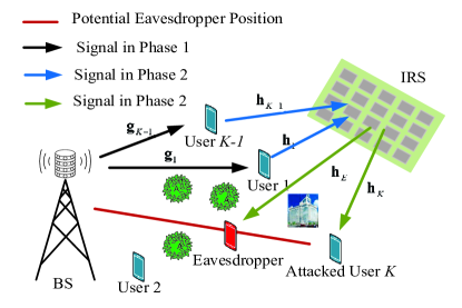
Figure 1: Two-phase communication system

As shown in Fig. 1, we consider Rician wiretap channels where a BS with $N$ transmit antennas communicates with $K$ single-antenna LUs in the presence of a single-antenna ED. An IRS with $M$ reflection elements is introduced to aid the secure communication.

II-A Channel Model

Figure 2: Coordinates of communication nodes in the system

Define the set of all LUs as $\mathcal{K}=\{1,2,...,K\}$, and denote set $\mathcal{K}_{-K}=\mathcal{K}/\{K\}$ and set $\mathcal{K}_{+E}=\mathcal{K}\cup\{E\}$. By denoting $\{D_{i},\theta_{i}\}_{\forall i\in\mathcal{\mathcal{K}}_{+E}}$ as the distances and the azimuth angles respectively from the BS to the LUs and the ED, as shown in Fig. 1, then the corresponding channels $\{\mathbf{g}_{i}\in\mathbb{C}^{N\times 1}\}_{\forall i\in\mathcal{\mathcal{K}}_{+E}}$ follow the Rician fading distribution [15]:

$$\mathbf{g}_{i}=\sqrt{\varrho_{0}\left(\frac{D_{i}}{d_{0}}\right)^{-\alpha_{\mathrm{BS}}}}\Biggl{(}\sqrt{\frac{K_{\mathrm{BS}}}{1+K_{\mathrm{BS}}}}\mathbf{g}_{i}^{\mathrm{LOS}}+\sqrt{\frac{1}{1+K_{\mathrm{BS}}}}\mathbf{g}_{i}^{\mathrm{NLOS}}\Biggr{)},\forall i\in\mathcal{K}_{+E},$$ (1)

where $\varrho_{0}$ is the pathloss at the reference distance of $d_{0}$, $\alpha_{BS}$ and $K_{BS}$ are the pathloss exponent and the Rician factor of the BS-related links, respectively. It is assumed that the BS is equipped with a uniform linear array (ULA). Then, the line-of-sight (LoS) component is given by $\mathbf{g}_{i}^{\mathrm{LOS}}=\left[1,e^{-\mathrm{j}\pi\sin\theta_{i}},\cdots,e^{-\mathrm{j}(N-1)\pi\sin\theta_{i}}\right]$, and the non-LoS component is drawn from a Rayleigh fading, i.e., $\mathbf{g}_{i}^{\mathrm{NLOS}}\sim\mathcal{CN}(\mathbf{0},\mathbf{I}_{N})$.

Furthermore, by denoting $\{D_{\mathrm{IRS}},\theta_{\mathrm{IRS}}\}$ as the distance and the azimuth angle from the BS to the IRS, it is straightforward to obtain the distances $\{d_{\mathrm{IRS},i}\}_{\forall i\in\mathcal{\mathcal{K}}_{+E}}$ and the azimuth angles $\{\varphi_{i}\}_{\forall i\in\mathcal{\mathcal{K}}_{+E}}$ from the IRS to the LUs and the ED as shown in Fig. 2, i.e.,

$$d_{\mathrm{IRS},i} =\Bigl{[}(D_{\mathrm{IRS}}\cos\theta_{\mathrm{IRS}}-D_{i}\cos\theta_{i})^{2}+(D_{\mathrm{IRS}}\sin\theta_{\mathrm{IRS}}-D_{i}\sin\theta_{i})^{2}\Bigr{]}^{-1/2},$$

$$\sin\varphi_{i} =\frac{1}{d_{\mathrm{IRS},i}}(D_{i}\sin\theta_{i}-D_{\mathrm{IRS}}\sin\theta_{\mathrm{IRS}}),$$

$$\cos\varphi_{i} =\frac{1}{d_{\mathrm{IRS},i}}(D_{\mathrm{IRS}}\cos\theta_{\mathrm{IRS}}-D_{i}\cos\theta_{i}).$$

The corresponding channels $\{\mathbf{h}_{i}\in\mathbb{C}^{N\times 1}\}_{\forall i\in\mathcal{\mathcal{K}}_{+E}}$ are given by

$$\mathbf{h}_{i} =\sqrt{\varrho_{0}\left(\frac{d_{\mathrm{IRS},i}}{d_{0}}\right)^{-\alpha_{\mathrm{IRS}}}}\Biggl{(}\sqrt{\frac{K_{\mathrm{IRS}}}{1+K_{\mathrm{IRS}}}}\mathbf{h}_{i}^{\mathrm{LOS}}+\sqrt{\frac{1}{1+K_{\mathrm{IRS}}}}\mathbf{h}_{i}^{\mathrm{NLOS}}\Biggr{)},\forall i\in\mathcal{K}_{+E},$$ (2)

where $\alpha_{\mathrm{IRS}}$ and $K_{\mathrm{IRS}}$ are the pathloss exponent and the Rician factor of the IRS-related links, respectively. The non-LoS component follows the distribution of $\mathbf{h}_{i}^{\mathrm{NLOS}}\sim\mathcal{CN}(\mathbf{0},\mathbf{I}_{M})$. It is assumed that the IRS is an uniform plane array (UPA) with size of $M=M_{{\rm x}}M_{{\rm y}}$, where $M_{{\rm x}}$ and $M_{{\rm y}}$ are the number of reflection elements in x-axis and y-axis, respectively. Then, the LoS component is written as

$$\mathbf{h}_{i}^{\mathrm{LOS}}=[1,\cdots,e^{-\mathrm{j}\pi(x\cos\varphi_{i}\cos\phi+y\sin\varphi_{i}\cos\phi)\sin\theta_{i}},\cdots,e^{-\mathrm{j}\pi((M_{{\rm x}}-1)\cos\varphi_{i}\cos\phi+(M_{y}-1)\sin\varphi_{i}\cos\phi)\sin\theta_{i}}],$$

where $1\leq x\leq M_{{\rm x}}$, $1\leq y\leq M_{{\rm y}}$ and $\phi$ is the elevation angle observed at the IRS side.

II-B Signal Transmission

To achieve high success rate of attack, the ED can locate the line between the BS and legitimate user. In this situation, the signal received by the ED is highly correlated with that of this user [11, 12], thus posing great threats to the system. As shown in Fig. 1, we assume that the ED hides at the line connecting the BS and one of the users, denoted as user $K$, which leads to $\theta_{E}\approx\theta_{K}$, $\mathbf{g}_{E}^{\mathrm{LOS}}\approx\mathbf{g}_{K}^{\mathrm{LOS}}$ and $D_{E}\in(0,D_{K})$. When the Rician factor $K_{\mathrm{BS}}$ is sufficiently large, the channel $\mathbf{g}_{E}$ is approximately equal to the channel $\mathbf{g}_{K}$.

In order to achieve high-quality secure communication, the angle aware user cooperation (AAUC) scheme [15] is adopted here. In particular, in the first phase, the BS multicasts the common signal to all users except user $K$. In the second phase, the helping users $(\forall k\in\mathcal{K}_{-K})$ forward the decoded common signal to user $K$ via the IRS. In this work, in order to implement the AAUC scheme without consuming extra energy, the LUs adopt the hybrid information and energy harvesting receiving mode which splits the received signal into two power streams with power splitting ratios $t_{k}$ and $1-t_{k}$. The former is used for decoding the signal and the latter is for energy harvesting.

II-B1 Multicasting Phase

In this phase, the BS multicasts the signal $s$ to the helping LUs through beamforming vector ${\bf f}\in\mathbb{C}^{N\times 1}$ which is limited to the maximum transmit power $P_{\max}$, i.e., $||{\bf f}||_{2}^{2}\leq P_{\max}$. Since $\mathbf{g}_{E}\approx\mathbf{g}_{K}$, the beamforming ${\bf f}$ needs to satisfy $|\mathbf{g}_{K}^{\mathrm{H}}{\bf f}|=0$ to ensure that $|\mathbf{g}_{E}^{\mathrm{H}}{\bf f}|\approx 0$. Let $\mathbf{Q}\in\mathbb{C}^{N\times\text{(}N-1)}$ be the orthogonal matrix which spans the null space of $\mathbf{g}_{K}$ by using the QR decomposition, i.e., $\mathbf{Q}^{\mathrm{H}}\mathbf{Q}={\bf I}$. Then, we can design ${\bf f}=\mathbf{Q}\mathbf{z}$, where $\mathbf{z}\in\mathbb{C}^{\text{(}N-1)\times 1}$ is a newly introduced variable. Therefore, the signal received by LU $k$ is given by $\mathbf{g}_{k}^{\mathrm{H}}\mathbf{Q}\mathbf{z}+n_{k}$, where $n_{k}$ is the received noise with the noise power of $\sigma_{k}^{2}$. By adopting the hybrid receiving mode and let ${\bf{t}}=[t_{1},...,t_{K-1}]^{{\rm{T}}}$ where $t_{k}$ is the power splitting ratio of LU $k$, the achievable rate at LU $k\neq K$ is

$$R_{k}\left({\bf z},t_{k}\right)=\frac{1}{2}\log_{2}\left(1+\frac{t_{k}}{\sigma_{k}^{2}}\left|\mathbf{g}_{k}^{\mathrm{H}}\mathbf{Q}\mathbf{z}\right|^{2}\right),$$ (3)

where the factor 1/2 is due to the two transmission phases. The harvested power at LU $k\neq K$ is

$$(1-t_{k})\left|\mathbf{g}_{k}^{\mathrm{H}}\mathbf{Q}\mathbf{z}\right|^{2}.$$ (4)

II-B2 User Cooperation Phase

In this phase, the helping LUs $(\forall k\in\mathcal{K}_{-K})$ forward the signal $s$ to LU $K$ through a beamforming vector ${\bf w}\in\mathbb{C}^{(K-1)\times 1}=[w_{1},...,w_{K-1}]^{\mathrm{T}}$ by using the power harvested in the multicasting phase. Since LU $K$ is randomly selected by the ED and assume that there are many obstacles in the communication environment, such as indoor applications, the direct links between the helping LUs and the LU $K$ may be blocked. To address this issue, an IRS can be installed on the building with a certain height, and thus the IRS is capable of reflecting the signals forwarded by the helping LUs to LU $K$. Denote by $\mathbf{e}$ the reflection coefficient vector of the IRS, where $|e_{m}|^{2}=1,\forall m=1,\cdots,M$. Then, the signal received by LU $K$ is given by

$$y_{K} =\mathbf{h}_{K}^{\mathrm{H}}\mathrm{diag}(\mathbf{e}^{*})\mathbf{H}_{\mathrm{IRS}}\mathbf{w}s+\sigma_{K}^{2}$$

$$=\mathbf{e}^{\mathrm{H}}\mathbf{H}_{K}\mathbf{w}s+\sigma_{K}^{2},$$

where $\mathbf{H}_{\mathrm{IRS}}=\left[\mathbf{h}_{1}\text{,\thinspace\thinspace...,\thinspace\thinspace$\mathbf{h}_{K-1}$}\right]$, $\mathbf{H}_{K}=\left[\mathbf{h}_{K}^{*}\odot\mathbf{h}_{1}\text{,\thinspace\thinspace...,\thinspace\thinspace$\mathbf{h}_{K}^{*}\odot\mathbf{h}_{K-1}$}\right]$ is the cascaded LU-IRS-LU (LIL) channel, and $n_{K}\sim\mathcal{CN}(\mathbf{0},\sigma_{K}^{2})$ is the noise. The corresponding achievable rate is

$$R_{K}\left(\mathbf{w},\mathbf{e}\right)=\frac{1}{2}\log_{2}\left(1+\frac{1}{\sigma_{K}^{2}}\left|\mathbf{e}^{\mathrm{H}}\mathbf{H}_{K}\mathbf{w}\right|^{2}\right).$$ (5)

On the other hand, the signal recieved by the ED is $y_{E}=\mathbf{e}^{\mathrm{H}}\mathbf{H}_{E}\mathbf{w}s+n_{E}$, where $\mathbf{H}_{E}=\left[\mathbf{h}_{E}^{*}\odot\mathbf{h}_{1}\text{,\thinspace\thinspace...,\thinspace\thinspace$\mathbf{h}_{E}^{*}\odot\mathbf{h}_{K-1}$}\right]$ is the cascaded LU-IRS-ED (LIE) channel, and $n_{E}\sim\mathcal{CN}(\mathbf{0},\sigma_{E}^{2})$ is the received noise at the ED.

The corresponding eavesdropping rate is

$$R_{E}\left(\mathbf{w},\mathbf{e}\right)=\frac{1}{2}\log_{2}\left(1+\frac{1}{\sigma_{E}^{2}}\left|\mathbf{e}^{\mathrm{H}}\mathbf{H}_{E}\mathbf{w}\right|^{2}\right).$$ (6)

Finally, the secrecy rate of this system under the AAUC scheme can be expressed as [12]:

$$\left[\min_{\forall k\in\mathcal{K}}R_{k}-R_{E}\right]^{+}.$$ (7)

In the following two sections, we consider the system design for two ED models: the active eavesdropper model and the passive eavesdropper model.

III ED Model I: Active Eavesdropper Model

In this section, we consider the active attack case, in which the ED pretends to be an LU sending pilot signals to the transmitters (including the BS and the helping LUs) during the channel estimation procedure [11, 12]. It is reasonable to assume that the BS is capable of addressing this attack by using the multi-antenna technique, so as to obtain perfect CSI of the system. Nevertheless, the signle-antenna helping LUs only have the imperfect CSI of LU $K$ and the ED due to their limited anti-interference ability.

III-A Channel Uncertainties

Based on the above assumption, the cascaded channels can be modeled as

$$\mathbf{H}_{K} =\widehat{\mathbf{H}}_{K}+\bm{\bigtriangleup}_{K},\thinspace\thinspace\mathbf{H}_{E}=\widehat{\mathbf{H}}_{E}+\bm{\bigtriangleup}_{E},$$ (8)

where $\widehat{\mathbf{H}}_{K}$ and $\widehat{\mathbf{H}}_{E}$ are the estimated cascaded channels, $\bm{\bigtriangleup}_{K}=[\bm{\bigtriangleup}_{1}^{K}\cdots\bm{\bigtriangleup}_{K-1}^{K}]$ and $\bm{\bigtriangleup}_{E}=[\bm{\bigtriangleup}_{1}^{E}\cdots\bm{\bigtriangleup}_{K-1}^{E}]$ are the unknown cascaded channel errors. $\bm{\bigtriangleup}_{k}^{K}$ and $\bm{\bigtriangleup}_{k}^{E}$ are the unknown cascaded LIL and LIE channel error vectors at LU $k$, respectively.

According to [13], the robust beamforming under the statistical CSI error model outperforms the bounded CSI error model in terms of the minimum transmit power, convergence speed and computational complexity. In addition, the statistical channel error model is more suitable to model the channel estimation error when the channel estimation is based on the minimum mean sum error (MMSE) method. Hence, we adopt the statistical model to characterize the cascadepd CSI imperfection [13], i.e., each CSI error vector is assumed to follow the circularly symmetric complex Gaussian (CSCG) distribution, i.e.,

$$\bm{\bigtriangleup}_{k}^{K} \sim\mathcal{CN}(\mathbf{0},\bm{\Sigma}_{k}^{K}),\bm{\Sigma}_{k}^{K}\succeq\mathbf{0},\forall k\in\mathcal{K}_{-K},$$ (9a)

$$\bm{\bigtriangleup}_{k}^{E} \sim\mathcal{CN}(\mathbf{0},\bm{\Sigma}_{k}^{E}),\bm{\Sigma}_{k}^{E}\succeq\mathbf{0},\forall k\in\mathcal{K}_{-K},$$ (9b)

where $\bm{\Sigma}_{k}^{K}\in\mathbb{C}^{M\times M}$ and $\bm{\Sigma}_{k}^{E}\in\mathbb{C}^{M\times M}$ are positive semidefinite error covariance matrices. Note that the CSI error vectors of different LUs are independent with each other. Therefore, we have

$$\mathrm{vec}(\bm{\bigtriangleup}_{K})\sim\mathcal{CN}(\mathbf{0},\bm{\Sigma}_{K}),\thinspace\thinspace\mathrm{vec}(\bm{\bigtriangleup}_{E})\sim\mathcal{CN}(\mathbf{0},\bm{\Sigma}_{E}),$$ (10)

where $\bm{\Sigma}_{K}$ and $\bm{\Sigma}_{E}$ are block diagonal matrices, i.e., $\bm{\Sigma}_{K}=\mathrm{diag}(\bm{\Sigma}_{1}^{K},...,\bm{\Sigma}_{K-1}^{K})$ and $\bm{\Sigma}_{E}=\mathrm{diag}(\bm{\Sigma}_{1}^{E},...,\bm{\Sigma}_{K-1}^{E})$.

III-B Outage constrained beamforming design

Under the statistical CSI error model, we develop a probabilistically robust algorithm for the secrecy rate maximization problem, which is formulated as

$$\max\limits_{R_{\mathrm{sec}},\mathbf{z},\mathbf{w},\mathbf{e},\mathbf{t}} R_{\mathrm{sec}}$$ (11a)

s.t. $$\mathrm{Pr}\left\{\min_{\forall k\in\mathcal{K}}R_{k}-R_{E}\geq R_{\mathrm{sec}}\right\}\geq 1-\rho$$ (11b)

$$||{\bf z}||_{2}^{2}\leq P_{\max}$$ (11c)

$$\;|e_{m}|^{2}=1,1\leq m\leq M$$ (11d)

$$0\leq\mathbf{t}\leq 1$$ (11e)

$$|w_{k}|^{2}\leq(1-t_{k})\left|\mathbf{g}_{k}^{\mathrm{H}}\mathbf{Q}\mathbf{z}\right|^{2},\forall k\in\mathcal{K}_{-K},$$ (11f)

where $\rho\in(0,1]$ is the secrecy rate outage probability.

Problem (11) is difficult to solve due to the computationally intractable rate outage probability constraint (11b), the non-convex unit-modulus constraint (11d), and the non-convex power constraint (11f).

Firstly, we replace constraint (11b) with the development of a safe approximation consisting of three steps in the following.

Step 1: Decouple the Probabilistic Constraint: First of all, based on the independence between $\{\mathbf{g}_{k}\}_{\forall k\in\mathcal{K}_{-K}}$ and $\mathbf{H}_{K}$, we have

$$(\ref{eq:r-c})\Leftrightarrow \prod_{k=1}^{K}\mathrm{Pr}\left\{R_{k}-R_{E}\geq R_{\mathrm{sec}}\right\}\geq 1-\rho$$ (12)

$$\Leftarrow \mathrm{Pr}\left\{R_{k}-R_{E}\geq R_{\mathrm{sec}}\right\}\geq 1-\bar{\rho},\forall k\in\mathcal{K}_{K},$$ (13)

where $\bar{\rho}=1-(1-\rho)^{1/K}$.

Step 2: Convenient Approximations: To address the non-concavity of $R_{k}-R_{E},\forall k\in\mathcal{K}_{K}$, we need to construct a sequence of surrogate functions of $\{R_{i}\}_{\forall i\in\mathcal{K}_{+E}}$. More specifically, we need the following lemmas.

Lemma 1

[16] The quadratic-over-linear function $\frac{x^{2}}{y}$ is jointly convex in $(x,y)$, and lower bounded by its linear first-order Tayler approximation $\frac{2x^{(n)}}{y^{(n)}}x-(\frac{x^{(n)}}{y^{(n)}})^{2}y$ at fixed point $(x^{(n)},y^{(n)})$.

By substituting $x$ with $\mathbf{g}_{k}^{\mathrm{H}}\mathbf{Q}\mathbf{z}$ and $y$ with $1/t_{k}$, we utilize Lemma 1 to obtain a concave lower bound of rate $R_{k}\left(\mathbf{z},t_{k}\right)$ for $\forall k\in\mathcal{K}_{-K}$. The lower bound is given by

$$\widetilde{R}_{k}(\mathbf{z},t_{k}|\mathbf{z}^{(n)},t_{k}^{(n)})=\frac{1}{2}\log_{2}\Biggl{(}1-\frac{t_{k}^{(n),2}}{\sigma_{k}^{2}t_{k}}\left|\mathbf{g}_{k}^{\mathrm{H}}\mathbf{Q}\mathbf{z}^{(n)}\right|^{2}+2t_{k}^{(n)}\mathrm{Re}\left\{\frac{1}{\sigma_{k}^{2}}{\bf z}^{(n),\mathrm{H}}\mathbf{Q}^{\mathrm{H}}\mathbf{g}_{k}\mathbf{g}_{k}^{\mathrm{H}}\mathbf{Q}\mathbf{z}\right\}\Biggr{)}$$ (14)

for any feasible solution $\{\mathbf{z}^{(n)},t_{k}^{(n)}\}$.

Lemma 2

The upper bound of rate $R_{E}\left(\mathbf{w},\mathbf{e}\right)$ is given by

$$\widetilde{R}_{E}\left(\mathbf{w},\mathbf{e},a_{E}\right) =\frac{a_{E}\left|\mathbf{e}^{\mathrm{H}}\mathbf{H}_{E}\mathbf{w}\right|^{2}/\sigma_{E}^{2}+a_{E}-\ln a_{E}-1}{2\ln 2},$$

where $a_{E}$ is the auxiliary variable.

Proof: See Appendix A.                                       $\blacksquare$

Lemma 3

The lower bound of rate $R_{K}\left(\mathbf{w},\mathbf{e}\right)$ is given by

$$\widetilde{R}_{K}(\mathbf{w},\mathbf{e},a_{K},v)=\frac{1}{2\ln 2}(-a_{K}|v|^{2}|\mathbf{e}^{\mathrm{H}}\mathbf{H}_{K}\mathbf{w}|^{2}-\sigma_{K}^{2}a_{K}|v|^{2}+2a_{K}\text{Re}\left\{v\mathbf{e}^{\mathrm{H}}\mathbf{H}_{K}\mathbf{w}\right\}-a_{K}+\ln a_{K}+1),$$

where $a_{K}$ and $v$ are the auxiliary variables.

Proof: See Appendix B.                                       $\blacksquare$

For the convenience of derivations, we assume that $\bm{\Sigma}_{k}^{K}=\varepsilon_{K,k}^{2}\mathbf{I}_{M}$ and $\bm{\Sigma}_{k}^{E}=\varepsilon_{E,k}^{2}\mathbf{I}_{M}$, then $\bm{\Sigma}_{K}=\bm{\Lambda}_{K}\otimes\mathbf{I}_{M}$ where $\bm{\Lambda}_{K}=\mathrm{diag}(\varepsilon_{K,1}^{2},...,\varepsilon_{K,K-1}^{2})$, and $\bm{\Sigma}_{E}=\bm{\Lambda}_{E}\otimes\mathbf{I}_{M}$ where $\bm{\Lambda}_{E}=\mathrm{diag}(\varepsilon_{E,1}^{2},...,\varepsilon_{E,K-1}^{2})$. Furthermore, the error vectors in (10) can be rewritten as $\mathrm{vec}(\bm{\bigtriangleup}_{K})=\bm{\Sigma}_{K}^{\frac{1}{2}}\mathbf{i}_{K}$ where $\mathbf{i}_{K}\sim\mathcal{CN}(\mathbf{0},\mathbf{I}_{M(K-1)})$, and $\mathrm{vec}(\bm{\bigtriangleup}_{E})=\bm{\Sigma}_{E}^{\frac{1}{2}}\mathbf{i}_{E}$ where $\mathbf{i}_{E}\sim\mathcal{CN}(\mathbf{0},\mathbf{I}_{M(K-1)})$. Define $\mathbf{E}=\mathbf{e}\mathbf{e}^{\mathrm{H}}$ and $\mathbf{W}=\mathbf{w}\mathbf{w}^{\mathrm{H}}$. Combining (14) with Lemma 2, the secrecy rate outage probabilities for $\forall k\in\mathcal{K}_{-K}$ in (13) are equivalent to

$$\mathrm{Pr}\left\{R_{k}-R_{E}\geq R_{\mathrm{sec}}\right\}$$

$$\geq \mathrm{Pr}\left\{\widetilde{R}_{k}-\widetilde{R}_{E}\geq R_{\mathrm{sec}}\right\}$$

$$= \mathrm{Pr}\Bigl{\{}a_{E}\mathrm{Tr}\left(\mathbf{E}(\widehat{\mathbf{H}}_{E}+\bm{\bigtriangleup}_{E})\mathbf{W}(\widehat{\mathbf{H}}_{E}^{\mathrm{H}}+\bm{\bigtriangleup}_{E}^{\mathrm{H}})\right)-[2\ln 2(\widetilde{R}_{k}-R_{\mathrm{sec}})-a_{E}+\ln a_{E}+1]\sigma_{E}^{2}\leq 0\Bigr{\}}$$

$$= \mathrm{Pr}\left\{\mathbf{i}_{E}^{\mathrm{H}}\mathbf{U}_{E}\mathbf{i}_{E}+2\mathrm{Re}\left\{\mathbf{u}_{E}^{\mathrm{H}}\mathbf{i}_{E}\right\}+u_{k}\leq 0\right\},$$ (15)

where

$$\mathbf{U}_{E} =a_{E}\bm{\Sigma}_{E}^{\frac{1}{2}}(\mathbf{W}^{\mathrm{T}}\otimes\mathbf{E})\bm{\Sigma}_{E}^{\frac{1}{2}},$$ (16a)

$$\mathbf{u}_{E} =a_{E}\bm{\Sigma}_{E}^{\frac{1}{2}}\mathrm{vec}(\mathbf{E}\mathbf{\widehat{H}}_{E}\mathbf{W}),$$ (16b)

$$u_{k} =a_{E}\mathrm{Tr}\left(\mathbf{E}\mathbf{\widehat{H}}_{E}\mathbf{W}\widehat{\mathbf{H}}_{E}^{\mathrm{H}}\right)-[(\widetilde{R}_{k}-R_{\mathrm{sec}})2\ln 2-a_{E}+\ln a_{E}+1]\sigma_{E}^{2}.$$ (16c)

Combining Lemma 2 with Lemma 3, the secrecy rate outage probability for LU $K$ in (13) is equivalent to

$$\mathrm{Pr}\left\{R_{K}-R_{E}\geq R_{\mathrm{sec}}\right\}$$

$$\geq \mathrm{Pr}\left\{\widetilde{R}_{K}-\widetilde{R}_{E}\geq R_{\mathrm{sec}}\right\}$$

$$= \mathrm{Pr}\Bigl{\{}a_{K}|v|^{2}\mathrm{Tr}\left(\mathbf{E}(\widehat{\mathbf{H}}_{K}+\bm{\bigtriangleup}_{K})\mathbf{W}(\widehat{\mathbf{H}}_{K}^{\mathrm{H}}+\bm{\bigtriangleup}_{K}^{\mathrm{H}})\right)-2a_{K}\mathrm{Re}\left\{v\mathbf{e}^{\mathrm{H}}(\widehat{\mathbf{H}}_{K}+\bm{\bigtriangleup}_{K})\mathbf{w}\right\}+$$

$$\frac{a_{E}}{\sigma_{E}^{2}}\mathrm{Tr}\left(\mathbf{E}(\widehat{\mathbf{H}}_{E}+\bm{\bigtriangleup}_{E})\mathbf{W}(\widehat{\mathbf{H}}_{E}^{\mathrm{H}}+\bm{\bigtriangleup}_{E}^{\mathrm{H}})\right)-c\leq 0\Bigr{\}}$$

$$= \mathrm{Pr}\left\{\mathbf{i}^{\mathrm{H}}\mathbf{U}_{K}\mathbf{i}+2\mathrm{Re}\left\{\mathbf{u}_{K}^{\mathrm{H}}\mathbf{i}\right\}+u_{K}\leq 0\right\},$$ (17)

where

$$\mathbf{i} =[\begin{array}[]{cc}\mathbf{i}_{K}^{\mathrm{H}},&\mathbf{i}_{E}^{\mathrm{H}}\end{array}]^{\mathrm{H}},$$ (18b)

$$\mathbf{U}_{K} =\mathrm{diag}\Bigl{\{}a_{K}|v|^{2}\bm{\Sigma}_{K}^{\frac{1}{2}}(\mathbf{W}^{\mathrm{T}}\otimes\mathbf{E})\bm{\Sigma}_{K}^{\frac{1}{2}},\ \frac{a_{E}}{\sigma_{E}^{2}}\bm{\Sigma}_{E}^{\frac{1}{2}}(\mathbf{W}^{\mathrm{T}}\otimes\mathbf{E})\bm{\Sigma}_{E}^{\frac{1}{2}}\Bigr{\}},$$ (18c)

$$\mathbf{u}_{K} =[a_{K}|v|^{2}\mathrm{vec}^{\mathrm{H}}(\mathbf{E}\mathbf{\widehat{H}}_{K}\mathbf{W})\bm{\Sigma}_{K}^{\frac{1}{2}}-a_{K}v\mathrm{vec}^{\mathrm{H}}(\mathbf{e}\mathbf{w}^{\mathrm{H}})\bm{\Sigma}_{K}^{\frac{1}{2}},\ \frac{a_{E}}{\sigma_{E}^{2}}\mathrm{vec}^{\mathrm{H}}(\mathbf{E}\mathbf{\widehat{H}}_{E}\mathbf{W})\bm{\Sigma}_{E}^{\frac{1}{2}}]^{\mathrm{H}},$$ (18d)

$$u_{K} =a_{K}|v|^{2}\mathrm{Tr}\left(\mathbf{E}\mathbf{\widehat{H}}_{K}\mathbf{W}\widehat{\mathbf{H}}_{K}^{\mathrm{H}}\right)+\frac{a_{E}}{\sigma_{E}^{2}}\mathrm{Tr}\left(\mathbf{E}\mathbf{\widehat{H}}_{E}\mathbf{W}\widehat{\mathbf{H}}_{E}^{\mathrm{H}}\right)\ -2a_{K}\mathrm{Re}\left\{v\mathbf{e}^{\mathrm{H}}\mathbf{\widehat{H}}_{K}\mathbf{w}\right\}-c,$$ (18e)

$$c =\ln a_{E}+\ln a_{K}-a_{E}-a_{K}-2R_{\mathrm{sec}}\ln 2\ -\sigma_{K}^{2}a_{K}|v|^{2}+2.$$ (18f)

Now, substituting (15) and (17) into (13), then (13) is replaced by

$$\mathrm{Pr}\left\{\mathbf{i}_{E}^{\mathrm{H}}\mathbf{U}_{E}\mathbf{i}_{E}+2\mathrm{Re}\left\{\mathbf{u}_{E}^{\mathrm{H}}\mathbf{i}_{E}\right\}+u_{k}\leq 0\right\}\geq 1-\bar{\rho},\forall k\in\mathcal{K}_{-K},$$ (19a)

$$\mathrm{Pr}\left\{\mathbf{i}^{\mathrm{H}}\mathbf{U}_{K}\mathbf{i}+2\mathrm{Re}\left\{\mathbf{u}_{K}^{\mathrm{H}}\mathbf{i}\right\}+u_{K}\leq 0\right\}\geq 1-\bar{\rho}.$$ (19b)

Step 3: A Bernstein-Type Inequality-Based Safe Approximation: The outage probabilities in (19) are characterized by quadratic inequalities, which can be safely approximated by using the following lemma.

Lemma 4

(Bernstein-Type Inequality) [17] Assume $f(\mathbf{x})=\mathbf{x}^{\mathrm{H}}\mathbf{U}\mathbf{x}+2\mathrm{Re}\{\mathbf{u}^{\mathrm{H}}\mathbf{x}\}+u$, where $\mathbf{U}\in\mathbb{H}^{n\times n}$, $\mathbf{u}\in\mathbb{C}^{n\times 1}$, $u\in\mathbb{R}$ and $\mathbf{x}\in\mathbb{C}^{n\times 1}\sim\mathcal{CN}(\mathbf{0},\mathbf{I})$. Then for any $\rho\in[0,1]$, the following approximation holds:

$$\mathrm{Pr}\{\mathbf{x}^{\mathrm{H}}\mathbf{U}\mathbf{x}+2\mathrm{Re}\{\mathbf{u}^{\mathrm{H}}\mathbf{x}\}+u\leq 0\}\geq 1-\rho$$

$$\Rightarrow \mathrm{Tr}\left\{\mathbf{U}\right\}+\sqrt{2\ln(1/\rho)}x-\ln(\rho)\lambda_{\max}^{+}(\mathbf{U})+u\leq 0$$

$$\Rightarrow \left\{\begin{array}[]{c}\mathrm{Tr}\left\{\mathbf{U}\right\}+\sqrt{2\ln(1/\rho)}x-\ln(\rho)y+u\leq 0\\ \sqrt{||\mathbf{U}||_{F}^{2}+2||\mathbf{u}||_{2}^{2}}\leq x\\ y\mathbf{I}-\mathbf{U}\succeq\mathbf{0},y\geq 0,\end{array}\right.$$ (23)

where $\lambda_{\max}^{+}(\mathbf{U})=\max(\lambda_{\max}(\mathbf{U}),0)$. $x$ and $y$ are slack variables.                                                         $\blacksquare$

Before using Lemma 4, we need the following simplified derivations for LU $k$, $\forall k\in\mathcal{K}_{-K}$, i.e.,

$$\mathrm{Tr}\left\{\mathbf{U}_{E}\right\}=\mathrm{Tr}\left\{a_{E}\bm{\Sigma}_{E}^{\frac{1}{2}}(\mathbf{W}^{\mathrm{T}}\otimes\mathbf{E})\bm{\Sigma}_{E}^{\frac{1}{2}}\right\}$$

$$\ \ \ \ \ \ \ \ \ \ =\mathrm{Tr}\left\{a_{E}(\mathbf{W}^{\mathrm{T}}\otimes\mathbf{E})(\bm{\Lambda}_{E}\otimes\mathbf{I}_{M})\right\}$$

$$\ \ \ \ \ \ \ \ \ \ =a_{E}M\mathrm{Tr}\left\{\bm{\Lambda}_{E}\mathbf{W}\right\},$$ (24a)

$$||\mathbf{U}_{E}||_{F}^{2}=a_{E}^{2}M^{2}||\bm{\Lambda}_{E}\mathbf{W}||_{F}^{2},$$ (24b)

$$||\mathbf{u}_{E}||_{2}^{2}=a_{E}^{2}\mathrm{vec}^{\mathrm{H}}(\mathbf{E}\mathbf{\widehat{H}}_{E}\mathbf{W})(\bm{\Lambda}_{E}\otimes\mathbf{I}_{M})\mathrm{vec}(\mathbf{E}\mathbf{\widehat{H}}_{E}\mathbf{W})$$

$$\ \ \ \ \ \ \ =a_{E}^{2}M||\bm{\Lambda}_{E}^{\frac{1}{2}}\mathbf{W}\mathbf{\widehat{H}}_{E}^{\mathrm{H}}\mathbf{e}||_{2}^{2},$$ (24c)

$$\lambda_{\max}(\mathbf{U}_{E})=\lambda_{\max}(a_{E}\bm{\Sigma}_{E}^{\frac{1}{2}}(\mathbf{W}^{\mathrm{T}}\otimes\mathbf{E})\bm{\Sigma}_{E}^{\frac{1}{2}})$$

$$\ \ \ \ \ \ \ \ \ \ \ \ =\lambda_{\max}(a_{E}(\bm{\Lambda}_{E}\mathbf{W}^{\mathrm{T}}\otimes\mathbf{E}))$$

$$\ \ \ \ \ \ \ \ \ \ \ \ =a_{E}\lambda_{\max}(\bm{\Lambda}_{E}\mathbf{W})\lambda(\mathbf{E})=a_{E}M\mathbf{w}^{\mathrm{H}}\bm{\Lambda}_{E}\mathbf{w}.$$ (24d)

By substituting (24) into (23) and introducing slack variables $\{x_{E},y_{E}\}$, the constraints for $\forall k\in\mathcal{K}_{-K}$ in (19a) are transformed into the following deterministic form:

$$\textrm{BTI}_{1}\triangleq\left\{\begin{array}[]{c}\mathrm{Tr}\left\{\mathbf{U}_{E}\right\}+\sqrt{2\ln(1/\bar{\rho})}x_{E}-\ln(\bar{\rho})y_{E}\\ +u_{k}\leq 0,\forall k\in\mathcal{K}_{-K}\\ \left\|\begin{array}[]{c}a_{E}M\mathrm{vec}(\bm{\Lambda}_{E}\mathbf{W})\\ \sqrt{2M}a_{E}\bm{\Lambda}_{E}^{\frac{1}{2}}\mathbf{W}\mathbf{\widehat{H}}_{E}^{\mathrm{H}}\mathbf{e}\end{array}\right\|\leq x_{E}\\ y_{E}\geq a_{E}M\mathbf{w}^{\mathrm{H}}\bm{\Lambda}_{E}\mathbf{w}.\end{array}\right.$$ (31)

On the other hand, the simplified derivations for LU $K$ are given by

$$\mathrm{Tr}\left\{\mathbf{U}_{K}\right\}=a_{K}|v|^{2}M\mathrm{Tr}\left\{\bm{\Lambda}_{K}\mathbf{W}\right\}+\frac{a_{E}}{\sigma_{E}^{2}}M\mathrm{Tr}\left\{\bm{\Lambda}_{E}\mathbf{W}\right\},$$ (32a)

$$||\mathbf{U}_{K}||_{F}^{2}=a_{K}^{2}|v|^{4}M^{2}||\bm{\Lambda}_{K}\mathbf{W}||_{F}^{2}+\frac{a_{E}^{2}}{\sigma_{E}^{4}}M^{2}||\bm{\Lambda}_{E}\mathbf{W}||_{F}^{2},$$ (32b)

$$||\mathbf{u}_{K}||^{2}=M||\bm{\Lambda}_{K}^{\frac{1}{2}}\left(a_{K}|v|^{2}\mathbf{W}\mathbf{\widehat{H}}_{K}^{\mathrm{H}}\mathbf{e}-a_{K}v\mathbf{w}\right)||_{2}^{2}+\frac{a_{E}^{2}}{\sigma_{E}^{4}}M||\mathbf{e}^{\mathrm{H}}\mathbf{\widehat{H}}_{E}\mathbf{W}\bm{\Lambda}_{E}^{\frac{1}{2}}||_{2}^{2},$$ (32c)

$$\lambda_{\max}(\mathbf{U}_{K})=\max\left\{a_{K}|v|^{2}M\mathbf{w}^{\mathrm{H}}\bm{\Lambda}_{K}\mathbf{w},\thinspace\thinspace\thinspace\frac{a_{E}}{\sigma_{E}^{2}}M\mathbf{w}^{\mathrm{H}}\bm{\Lambda}_{E}\mathbf{w}\right\}.$$

By substituting the above equations into (23) and introducing slack variables $\{x_{K},y_{K}\}$, the constraint for LU $K$ in (19b) is transformed into the following deterministic form:

$$\textrm{BTI}_{2}\triangleq\left\{\begin{array}[]{c}\mathrm{Tr}\left\{\mathbf{U}_{K}\right\}+\sqrt{2\ln(1/\bar{\rho})}x_{K}-\ln(\bar{\rho})y_{K}+u_{K}\leq 0\\ \left\|\begin{array}[]{c}a_{K}|v|^{2}M\mathrm{vec}(\bm{\Lambda}_{K}\mathbf{W})\\ a_{E}M\mathrm{vec}(\bm{\Lambda}_{E}\mathbf{W})/\sigma_{E}^{2}\\ \sqrt{2M}\bm{\Lambda}_{K}^{\frac{1}{2}}\left(a_{K}|v|^{2}\mathbf{W}\mathbf{\widehat{H}}_{K}^{\mathrm{H}}\mathbf{e}-a_{K}v\mathbf{w}\right)\\ \sqrt{2M}a_{E}\bm{\Lambda}_{E}^{\frac{1}{2}}\mathbf{W}\mathbf{\widehat{H}}_{E}^{\mathrm{H}}\mathbf{e}/\sigma_{E}^{2}\end{array}\right\|\leq x_{K}\\ y_{K}\geq\lambda_{\max}(\mathbf{U}_{K}),y_{K}\geq 0.\end{array}\right.$$ (40)

Then, to handle the non-convex power constraint (11f), we replace the right hand side of (11f) with its linear lower bound

$$\Xi({\bf z},t_{k})= 2(1-t_{k}^{(n)})\mathrm{Re}\left\{{\bf z}^{(n),\mathrm{H}}\mathbf{Q}^{\mathrm{H}}\mathbf{g}_{k}\mathbf{g}_{k}^{\mathrm{H}}\mathbf{Q}\mathbf{z}\right\}-\frac{(1-t_{k}^{(n)})^{2}\left|\mathbf{g}_{k}^{\mathrm{H}}\mathbf{Q}\mathbf{z}^{(n)}\right|^{2}}{(1-t_{k})}$$ (41)

at feasible point $\{\mathbf{z}^{(n)},t_{k}^{(n)}\}$ by adopting the same first-order Taylor approximation used in Lemma 1.

Therefore, based on (31), (40) and (41) and denoting $\mathbf{x}=[x_{E},x_{K}]^{\mathrm{T}}$and $\mathbf{y}=[y_{E},y_{K}]^{\mathrm{T}}$, the approximation problem of Problem (11) is given by

$$\max\limits_{R_{\mathrm{sec}},\mathbf{z},\mathbf{w},\mathbf{e},\mathbf{t},a_{K},a_{E},v,\mathbf{x},\mathbf{y}} R_{\mathrm{sec}}$$ (42a)

s.t. $$(\ref{eq:BTI-1}),(\ref{eq:BTI-2}),(\ref{eq:p-c})-(\ref{eq:sp-c}),$$ (42b)

$$|w_{k}|^{2}\leq\Xi({\bf z},t_{k}),\forall k\in\mathcal{K}_{-K}.$$ (42c)

For given $\{\mathbf{e},a_{K},a_{E},v\}$, we introduce a new variable $\mathbf{W}=\mathbf{w}\mathbf{w}^{\mathrm{H}}$ with $\mathrm{rank}(\mathbf{W})=1$. However, different from the general semidefinite programming (SDP), $\mathbf{w}$ and $\mathbf{W}$, here, coexist in (LABEL:eq:v) and (32c). Therefore, the semidefinite relaxation (SDR) technique is not applicable here. In order to handle this problem, we assume $\mathbf{w}$ and $\mathbf{W}$ are two different variables. If $\mathrm{Tr}\left\{\mathbf{W}\right\}=\lambda_{\max}(\mathbf{W})$, then we have $\mathrm{rank}(\mathbf{W})=1$. If the obtained $\mathbf{W}$ is not rank one, we will have $\mathrm{Tr}\left\{\mathbf{W}\right\}-\lambda_{\max}(\mathbf{W})>0$. Therefore, we constrain $\mathrm{Tr}\left\{\mathbf{W}\right\}-\lambda_{\max}(\mathbf{W})$ less than a very small real positive number threshold $\varepsilon$ to guarantee the rank-1 condition of $\mathbf{W}$, yielding the surrogate constraint of rank-1 constraint as

$$\mathrm{Tr}\left\{\mathbf{W}\right\}-\lambda_{\max}(\mathbf{W})\leq\varepsilon.$$ (43a)

When $\mathrm{rank}(\mathbf{W})\approx 1$, the relationship between $\mathbf{w}$ and $\mathbf{W}$ is given by the following constraint:

$$-\varepsilon\leq||\mathbf{w}||^{2}-\mathrm{Tr}\left\{\mathbf{W}\right\}\leq\varepsilon.$$ (44a)

As for constraint (43a), since $\lambda_{\max}(\mathbf{W})$ is a convex function of $\mathbf{W}$ [16], the left hand side of (43a) is concave, which is the difference between a linear function and a convex function. Hence, we need to construct a convex approximation of constraint (43a). To address this issue, we introduce the following lemma.

Lemma 5

Denote by $\mathbf{v}_{max}$ the eigenvector corresponding to the maximum eigenvalue of a matrix $\mathbf{V}$, we have

$$\mathrm{Tr}\left\{\mathbf{v}_{max}\mathbf{v}_{max}^{\mathrm{H}}(\mathbf{Z}-\mathbf{V})\right\} =\mathbf{v}_{max}^{\mathrm{H}}\mathbf{Z}\mathbf{v}_{max}-\mathbf{v}_{max}^{\mathrm{H}}\mathbf{V}\mathbf{v}_{max}$$

$$=\mathbf{v}_{max}^{\mathrm{H}}\mathbf{Z}\mathbf{v}_{max}-\lambda_{\max}(\mathbf{V})$$

$$\leq\lambda_{\max}(\mathbf{Z})-\lambda_{\max}(\mathbf{V})$$

for any Hermitian matrix $\mathbf{Z}$.                                                                                                        $\blacksquare$

Let $\mathbf{d}_{\mathbf{W}}^{(n)}$ be the eigenvector corresponding to the maximum eigenvalue of the feasible point $\mathbf{W}^{(n)}$. Then, by using Lemma 5, the surrogate convex constraint of (43a) is given by

$$\mathrm{Tr}\left\{\mathbf{W}\right\}-\lambda_{\max}(\mathbf{W}^{(n)})-\mathrm{Tr}\left\{\mathbf{d}_{\mathbf{W}}^{(n)}\mathbf{d}_{\mathbf{W}}^{(n),\mathrm{H}}(\mathbf{W}-\mathbf{W}^{(n)})\right\}\leq\varepsilon.$$ (45)

Now, we consider constraint (44a). By appying the first-order Tayler approximation to $||\mathbf{w}||^{2}$, we obtain the following convex approximation of the constraint in (44a) as

$$||\mathbf{w}||^{2}-\mathrm{Tr}\left\{\mathbf{W}\right\} \leq\varepsilon,$$ (46a)

$$2\mathrm{Re}\left\{\mathbf{w}^{(n),\mathrm{H}}\mathbf{w}\right\}-||\mathbf{w}^{(n)}||^{2}-\mathrm{Tr}\left\{\mathbf{W}\right\} \geq-\varepsilon.$$ (46b)

Finally, the subproblem w.r.t., $\{\mathbf{z},\mathbf{w},\mathbf{W},\mathbf{t}\}$ is formulated as

$$\max\limits_{R_{\mathrm{sec}},\mathbf{z},\mathbf{w},\mathbf{W},\mathbf{t},\mathbf{x},\mathbf{y}} R_{\mathrm{sec}}$$ (47a)

s.t. $$(\ref{eq:BTI-1}),(\ref{eq:BTI-2}),(\ref{eq:p-c}),(\ref{eq:sp-c}),$$ (47b)

$$(\ref{eq:ph2}),(\ref{Pro:W-c-1}),(\ref{Pro:W-c-2})$$ (47c)

$$\mathbf{W}\succeq\mathbf{0}.$$ (47d)

Problem (47) is an SDP and can be solved by the CVX tool [18].

For given $\{\mathbf{w},a_{K},a_{E},v\}$, Problem (42) with optimization variable $\mathbf{e}$ can be solved by applying the penalty CCP [13, 19, 20] to relax the unit-modulus constraint (11d). Comparing with the SDR technique, the penalty CCP method is capable of finding a feasible solution to meet constraint (11d). In particular, the constraint of (11d) can be relaxed by

$$|e_{m}^{[j]}|^{2}-2\mathrm{Re}(e_{m}^{\mathrm{H}}e_{m}^{[j]})\leq b_{m}-1,1\leq m\leq M,$$ (48a)

$$|e_{m}|^{2}\leq 1+b_{M+m},1\leq m\leq M,$$ (48b)

where $e_{m}^{[j]}$ is any feasible solution and $\mathbf{b}=[b_{1},...,b_{2M}]^{\mathrm{T}}$ is slack vector variable. The proof of (48) can be found in [13, 19]. Following the penalty CCP framework, the subproblem for optimizing $\mathbf{e}$ is formulated as

$$\max\limits_{R_{\mathrm{sec}},\mathbf{e},\mathbf{x},\mathbf{y}} R_{\mathrm{sec}}-\lambda^{[j]}||\mathbf{b}||_{1}$$ (49a)

s.t. $$(\ref{eq:BTI-1}),(\ref{eq:BTI-2}),(\ref{Pro:e-c-1}).$$ (49b)

Problem (49) is an SDP and can be solved by the CVX tool. The algorithm for finding a feasible solution of $\mathbf{e}$ is summarized in Algorithm 1.

Algorithm 1 Penalty CCP optimization for reflection beamforming optimization

0:  Initialize $\mathbf{e}^{[0]}$, $\gamma^{[0]}>1$, and set $j=0$.

1:  repeat

2:     if $j<J_{max}$ then

3:        Update $\mathbf{e}^{[j+1]}$ by solving Problem (49);

4:        Update $\lambda^{[j+1]}=\min\{\gamma\lambda^{[j]},\lambda_{max}\}$;

5:        $j=j+1$;

6:     else

7:        Initialize with a new random $\mathbf{e}^{[0]}$, set up $\gamma^{[0]}>1$ again, and set $j=0$.

8:     end if

9:  until $||\mathbf{b}||_{1}\leq\chi$ and $||\mathbf{e}^{[j]}-\mathbf{e}^{[j-1]}||_{1}\leq\nu$.

10:  Output $\mathbf{e}^{(n+1)}=\mathbf{e}^{[j]}$.

In addition, Problem (42) is convex in $\{R_{\mathrm{sec}},v,\mathbf{x},\mathbf{y}\}$ for given $\{\mathbf{z},\mathbf{w},\mathbf{e},\mathbf{t},a_{K},a_{E},\}$, and convex in $\{R_{\mathrm{sec}},a_{K},a_{E},\mathbf{x},\mathbf{y}\}$ for given $\{\mathbf{z},\mathbf{w},\mathbf{e},\mathbf{t},v,\}$. Finally, Problem (42) is addressed under the alternate optimization (AO) framework containing four subproblems. The convergence of the AO framework can be guaranteed due to the fact that each subproblem can obtain a non-decreasing sequence of objective function values.

IV ED Model II: Passive Eavesdropper Model

In this section, we focus on the transmission design for the passive attack, which is more practical and more challenging to address, since the passive ED can hide itself and its CSI is not known [11, 12]. The authors of [15] proposed to exploit the angular information of the ED to combat its passive attack, which is also applicable here. In this section, the cascaded LIL channel $\mathbf{H}_{K}$ and the channel $\mathbf{H}_{\mathrm{IRS}}$ are assumed to be perfect, which is reasonable due to the fact that the pilot information for channel estimation for LUs is known at the BS.

IV-A Average eavesdropping rate Maximization

The signal received by the ED is formulated as

$$y_{E} =\mathbf{h}_{E}^{\mathrm{H}}\mathrm{diag}(\mathbf{e}^{*})\mathbf{H}_{\mathrm{IRS}}\mathbf{w}s+\sigma_{E}^{2}.$$

Since the ED is passive, we can only detect the activity of the ED on the line segment between the BS and LU $K$ without knowing its exact location. This detection of a passive attack is based on spectrum sensing [21]. Hence, the average eavesdropping rate is considered which can be computed as follows [22, 23, 15]:

$$R_{E}^{av}\left(\mathbf{w},\mathbf{e}\right)=\frac{1}{D_{K}}\int_{0}^{D_{K}}\mathbb{E}_{\{\mathbf{h}_{E}\}}\Biggl{[}\frac{1}{2}\log_{2}\biggl{(}1+\frac{1}{\sigma_{E}^{2}}\left|\mathbf{h}_{E}^{\mathrm{H}}\mathrm{diag}(\mathbf{e}^{*})\mathbf{H}_{\mathrm{IRS}}\mathbf{w}\right|^{2}\biggr{)}\Biggr{]}\mathrm{d}_{D_{E}}.$$ (50)

With (50), we formulate the following optimization problem:

$$\max\limits_{\mathbf{z},\mathbf{w},\mathbf{e},\mathbf{t}} \left\{\min_{\forall k\in\mathcal{K}}R_{k}-R_{E}^{av}\left(\mathbf{w},\mathbf{e}\right)\right\}$$ (51a)

s.t. $$(\ref{eq:p-c})-(\ref{eq:ph-c}).$$ (51b)

The main challenge to solve Problem (51) is from the average eavesdropping rate containing the integration over $D_{E}$ and the expectation over $\mathbf{h}_{E}$. To address this issue, we use Jensen’s inequality to construct an upper bound of $R_{E}^{av}\left(\mathbf{w},\mathbf{e}\right)$ given by

$$R_{E}^{up}\left(\mathbf{w},\mathbf{e}\right) =\frac{1}{2}\log_{2}\left(1+\frac{\int_{0}^{D_{K}}\mathbb{E}_{\{\mathbf{h}_{E}\}}\left[\left|\mathbf{h}_{E}^{\mathrm{H}}\mathrm{diag}(\mathbf{e}^{*})\mathbf{H}_{\mathrm{IRS}}\mathbf{w}\right|^{2}\right]\mathrm{d}_{D_{E}}}{\sigma_{E}^{2}D_{K}}\right)$$

$$=\frac{1}{2}\log_{2}\left(1+\frac{1}{\sigma_{E}^{2}}\mathbf{w}^{\mathrm{H}}\mathbf{H}_{\mathrm{IRS}}^{\mathrm{H}}\mathrm{diag}(\mathbf{e})\mathbf{R}_{E}\mathrm{diag}(\mathbf{e}^{*})\mathbf{H}_{\mathrm{IRS}}\mathbf{w}\right),$$ (52)

where $\mathbf{R}_{E}=\frac{1}{D_{K}}\int_{0}^{D_{K}}\mathbb{E}_{\{\mathbf{h}_{E}\}}[\mathbf{h}_{E}\mathbf{h}_{E}^{\mathrm{H}}]\mathrm{d}_{D_{E}}$ which can be computed via one-dimension integration.

According to (2), we define

$$\overline{\mathbf{h}}_{E} =\sqrt{\varrho_{0}\left(\frac{d_{\mathrm{IRS},E}}{d_{0}}\right)^{-\alpha_{\mathrm{IRS}}}\frac{K_{\mathrm{IRS}}}{1+K_{\mathrm{IRS}}}}\mathbf{h}_{E}^{\mathrm{LOS}},$$ (53a)

$$\mathbf{R}_{E} =\varrho_{0}\left(\frac{d_{\mathrm{IRS},E}}{d_{0}}\right)^{-\alpha_{\mathrm{IRS}}}\frac{1}{1+K_{\mathrm{IRS}}}\mathbf{I}_{M},$$ (53b)

where $\overline{\mathbf{h}}_{E}$ describes the LoS component and is the mean of channel $\mathbf{h}_{E}$. Moreover, $\mathbf{R}_{E}$ is a positive semi-definite covariance matrix representing the spatial correlation characteristics of the NLoS component. Therefore, we have $\mathbf{h}_{E}\sim\mathcal{CN}(\overline{\mathbf{h}}_{E},\mathbf{R}_{E})$ [24], and further get

$$\mathbb{E}_{\{\mathbf{h}_{E}\}}[\mathbf{h}_{E}\mathbf{h}_{E}^{\mathrm{H}}] =\left[\mathbf{R}_{E}+\overline{\mathbf{h}}_{E}\overline{\mathbf{h}}_{E}^{\mathrm{H}}\right]$$

$$=\varrho_{0}\left(\frac{d_{\mathrm{IRS},E}}{d_{0}}\right)^{-\alpha_{\mathrm{IRS}}}\cdot\left[\frac{1}{1+K_{\mathrm{IRS}}}\mathbf{I}_{M}+\frac{K_{\mathrm{IRS}}}{1+K_{\mathrm{IRS}}}\mathbf{h}_{E}^{\mathrm{LOS}}(\mathbf{h}_{E}^{\mathrm{LOS}})^{\mathrm{H}}\right].$$

IV-B Proposed Algorithm

By replacing $R_{E}^{av}\left(\mathbf{w},\mathbf{e}\right)$ with $R_{E}^{up}\left(\mathbf{w},\mathbf{e}\right)$ in the objective function of Problem (51), we have

$$\max\limits_{\mathbf{z},\mathbf{w},\mathbf{e},\mathbf{t}} \left\{\min_{\forall k\in\mathcal{K}}R_{k}-R_{E}^{up}\right\}$$ (54a)

s.t. $$(\ref{eq:p-c})-(\ref{eq:ph-c}).$$ (54b)

Problem (54) is still difficult to solve due to the non-convex constraints and objective function, as well as the coupled variables $\mathbf{w}$ and $\mathbf{e}$. Hence, we propose an MM-based AO method to update $\mathbf{w}$ and $\mathbf{e}$ iteratively. More specifically, by first fixing $\mathbf{e}$, the non-concave objective function w.r.t., $\{{\bf z},\mathbf{w},\mathbf{t}\}$ is replaced by its customized concave surrogate function and then solved by the CVX. $\{{\bf z},\mathbf{w},\mathbf{t}\}$ are then fixed and the closed-form solution of $\mathbf{e}$ can be found by constructing an easy-to-solve surrogate objective function w.r.t $\mathbf{e}$.

The surrogate functions of $R_{k}\left(\mathbf{z},t_{k}\right)$ for $\forall k\in\mathcal{K}_{-K}$ are given by $\widehat{R}_{k}(\mathbf{z},t_{k}|\mathbf{z}^{(n)},t_{k}^{(n)})=\widetilde{R}_{k}(\mathbf{z},t_{k}|\mathbf{z}^{(n)},t_{k}^{(n)})$ given in (14), and those of $R_{K}\left(\mathbf{w},\mathbf{e}\right)$ and $R_{E}\left(\mathbf{w},\mathbf{e}\right)$ are given in the following lemma by using the first-order Taylor approximation.

Lemma 6

Let $\{\mathbf{w}^{(n)},\mathbf{e}^{(n)}\}$ be any feasible solution, then $R_{K}\left(\mathbf{w},\mathbf{e}\right)$ is lower bounded by a concave surrogate function $\widehat{R}_{K}\left(\mathbf{w},\mathbf{e}|\mathbf{w}^{(n)},\mathbf{e}^{(n)}\right)$ defined by

$$\widehat{R}_{K}(\mathbf{w},\mathbf{e}|\mathbf{w}^{(n)},\mathbf{e}^{(n)}) =\frac{1}{2}\log_{2}\Biggl{(}1-\frac{q_{K}^{(n)}}{\sigma_{K}^{2}}+2\mathrm{Re}\left\{\frac{q_{K}}{\sigma_{K}^{2}}\right\}\Biggr{)},$$ (55)

where $q_{K}^{(n)}=\left|\mathbf{e}^{(n),\mathrm{H}}\mathbf{H}_{K}\mathbf{w}^{(n)}\right|^{2}$ and $q_{K}=\mathbf{e}^{(n),\mathrm{H}}\mathbf{H}_{K}\mathbf{w}^{(n)}\mathbf{w}^{\mathrm{H}}\mathbf{H}_{K}^{\mathrm{H}}\mathbf{e}$.

Meanwhile, $R_{E}\left(\mathbf{w},\mathbf{e}\right)$ is upper bounded by a convex surrogate function $\widehat{R}_{E}\left(\mathbf{w},\mathbf{e}|\mathbf{w}^{(n)},\mathbf{e}^{(n)}\right)$ given by

$$\widehat{R}_{E}^{up}\left(\mathbf{w},\mathbf{e}|\mathbf{w}^{(n)},\mathbf{e}^{(n)}\right)=\frac{1}{2}\log_{2}\left(1+\frac{q_{E}^{(n)}}{\sigma_{E}^{2}}\right)+\frac{q_{E}-q_{E}^{(n)}}{2(\sigma_{E}^{2}+q_{E}^{(n)})\ln 2},$$ (56)

where $q_{E}^{(n)}=\mathbf{w}^{(n),\mathrm{H}}\mathbf{H}_{\mathrm{IRS}}^{\mathrm{H}}\mathrm{diag}(\mathbf{e}^{(n)})\mathbf{R}_{E}\mathrm{diag}(\mathbf{e}^{(n),*})\mathbf{H}_{\mathrm{IRS}}\mathbf{w}^{(n)}$ and $q_{E}=\mathbf{w}^{\mathrm{H}}\mathbf{H}_{\mathrm{IRS}}^{\mathrm{H}}\mathrm{diag}(\mathbf{e})\mathbf{R}_{E}\mathrm{diag}(\mathbf{e}^{*})\mathbf{H}_{\mathrm{IRS}}\mathbf{w}$.

Furthermore, we have the following proposition.

Proposition 1

The functions $\{\widehat{R}_{k},\widehat{R}_{K},\widehat{R}_{E}^{up}\}$ preserve the first-order property of functions $\{R_{k},R_{K},R_{E}\}$, respectively. Let’s take $\widehat{R}_{K}$ and $R_{K}$ as an example

$$\nabla_{\mathbf{w}}\widehat{R}_{K}(\mathbf{w},\mathbf{e}^{(n)}|\mathbf{w}^{(n)},\mathbf{e}^{(n)})|_{\mathbf{w}=\mathbf{w}^{(n)}}= \nabla_{\mathbf{w}}R_{K}\left(\mathbf{w},\mathbf{e}^{(n)}\right)|_{\mathbf{w}=\mathbf{w}^{(n)}},$$

$$\nabla_{\mathbf{e}}\widehat{R}_{K}(\mathbf{w}^{(n)},\mathbf{e}|\mathbf{w}^{(n)},\mathbf{e}^{(n)})|_{\mathbf{e}=\mathbf{e}^{(n)}}= \nabla_{\mathbf{e}}R_{K}\left(\mathbf{w}^{(n)},\mathbf{e}\right)|_{\mathbf{e}=\mathbf{e}^{(n)}}.$$

Proof: See Appendix B in [15].                                                                                              $\blacksquare$

Giving $\mathbf{e}$ and combining (14), (55), (56) and (42c), the subproblem of optimizing $\{{\bf z},\mathbf{w},\mathbf{t}\}$ is formulated as

$$\max\limits_{\mathbf{z},\mathbf{w},\mathbf{t}} \left\{\min_{\forall k\in\mathcal{K}}\widehat{R}_{k}-\widehat{R}_{E}^{up}\right\}$$ (57a)

s.t. $$(\ref{eq:p-c}),(\ref{eq:sp-c}),(\ref{eq:ph2}).$$ (57b)

Introducing auxiliary variable $r$, we can transform Problem (57) into

$$\max\limits_{\mathbf{z},\mathbf{w},\mathbf{t},r} \left\{r-\widehat{R}_{E}^{up}\right\}$$ (58a)

s.t. $$(\ref{eq:p-c}),(\ref{eq:sp-c}),(\ref{eq:ph2})$$ (58b)

$$\widehat{R}_{k}\geq r,\forall k\in\mathcal{K},$$ (58c)

which is convex and can be solved by using CVX.

Giving $\{{\bf z},\mathbf{w},\mathbf{t}\}$ and combining (14), (55) and (56), the subproblem w.r.t., $\mathbf{e}$ is formulated as

$$\max\limits_{\mathbf{e}} \left\{\min_{\forall k\in\mathcal{K}}\widehat{R}_{k}-\widehat{R}_{E}^{up}\right\},\textrm{s.t.}(\ref{eq:e-c}).$$ (59)

Problem (59) can be addressed by transforming it into an SOCP under the penalty CCP method mentioned in Section III-B. However, the penalty CCP method needs to solve a series of SOCP problems which incurs a high computational complexity. In the following, we aim to derive a low-complexity algorithm containing the closed-form solution of $\mathbf{e}$.

Denote by $\mathcal{R}=\min_{k=1}^{K-1}\left\{R_{k}\left(\mathbf{z},t_{k}\right)\right\}$ that is a constant, then the subproblem of Problem (54) corresponding to the optimization of $\mathbf{e}$ is given by

$$\max\limits_{\mathbf{e}} \left\{\min\{\mathcal{R},R_{K}\left(\mathbf{e}\right)\}-R_{E}^{up}\left(\mathbf{e}\right)\right\},\textrm{s.t.}(\ref{eq:e-c}).$$ (60)

Before solving Problem (60), we first consider the following two subproblems:

$$\mathcal{P}1:\thinspace\thinspace\thinspace\thinspace \min\limits_{\mathbf{e}}R_{E}^{up}\left(\mathbf{e}\right),\textrm{s.t.}(\ref{eq:e-c}),R_{K}\left(\mathbf{e}\right)\geq\mathcal{R}.$$ (61)

$$\mathcal{P}2:\thinspace\thinspace\thinspace\thinspace \max\limits_{\mathbf{e}}R_{K}\left(\mathbf{e}\right)-R_{E}^{up}\left(\mathbf{e}\right),\textrm{s.t.}(\ref{eq:e-c}),R_{K}\left(\mathbf{e}\right)\leq\mathcal{R}.$$ (62)

Denote the solutions to $\mathcal{P}1$ and $\mathcal{P}2$ as $\mathbf{e}_{1}^{\#}$ and $\mathbf{e}_{2}^{\#}$, respectively. In addition, let us denote the objective function value of Problem (60) as $obj(\mathbf{e})$, which is a function of $\mathbf{e}$. If $obj(\mathbf{e}_{1}^{\#})\geq obj(\mathbf{e}_{2}^{\#})$, then the optimal solution of Problem (60) is given by $\mathbf{e}_{1}^{\#}$. Otherwise, the optimal solution is $\mathbf{e}_{2}^{\#}$.

The solutions to Problem $\mathcal{P}1$ and Problem $\mathcal{P}2$ are given in the following lemma.

Lemma 7

The optimal solution of $\mathcal{P}1$ is given by

$$\mathbf{e}_{1}^{\#}=\exp\{\mathrm{j}\arg((\lambda_{\max}(\mathbf{A}_{E})\mathbf{I}-\mathbf{A}_{E}+\varrho_{1}^{opt}\mathbf{A}_{K})\mathbf{e}^{(n)})\},$$ (63)

where $\mathbf{A}_{E}=\text{($\mathbf{H}_{\mathrm{IRS}}$$\mathbf{w}\mathbf{w}^{\mathrm{H}}\mathbf{H}_{\mathrm{IRS}}^{\mathrm{H}}$)}\odot(\mathbf{R}_{E}^{\mathrm{T}}/\sigma_{E}^{2})$, $\mathbf{A}_{K}=\mathbf{H}_{K}\mathbf{w}\mathbf{w}^{\mathrm{H}}\mathbf{H}_{K}^{\mathrm{H}}/\sigma_{K}^{2}$ and $\varrho_{1}^{opt}$ is the price introduced by the price mechanism [25].

The optimal solution of $\mathcal{P}2$ is given by

$$\mathbf{e}_{2}^{\#}=\exp\{\mathrm{j}\arg(\mathbf{c}+\varrho_{2}^{opt}(\lambda_{\max}(\mathbf{A}_{K})\mathbf{I}-\mathbf{A}_{K})\mathbf{e}^{(n)})\},$$ (64)

where $\varrho_{2}^{opt}$ is the price and

$$\mathbf{c}=\frac{1+d_{K}^{(n)}}{(1+d_{E}^{(n)})^{2}}(\lambda_{\max}(\mathbf{A}_{E})\mathbf{I}-\mathbf{A}_{E})\mathbf{e}^{(n)}+\frac{\mathbf{A}_{K}\mathbf{e}^{(n)}}{1+d_{E}^{(n)}},$$

$$d_{K}^{(n)}=\mathbf{e}^{(n),\mathrm{H}}\mathbf{A}_{K}\mathbf{e}^{(n)},\thinspace\thinspace\thinspace\thinspace\thinspace\thinspace\thinspace\thinspace\thinspace\thinspace\thinspace\thinspace\thinspace d_{E}^{(n)}=\mathbf{e}^{(n),\mathrm{H}}\mathbf{A}_{E}\mathbf{e}^{(n)}.$$

Proof: See Appendix C.                                                                                                       $\blacksquare$

Since $\mathbf{e}_{1}^{\#}$ and $\mathbf{e}_{2}^{\#}$ are the globally optimal solutions of $\mathcal{P}1$ and $\mathcal{P}2$, respectively, hence $\mathbf{e}^{\#}$ is the globally optimal solution of Problem (60). The optimal price parameter can be obtained by using the bisection search method detailed in [25].

According to Proposition 1 and Theorem 1 in [26], the sequence $\{\mathbf{z}^{(n)},\mathbf{w}^{(n)},\mathbf{t}^{(n)},\mathbf{e}^{(n)}\}_{n=1,2,3,\ldots}$ obtained in each iteration is guaranteed to converge to the set of stationary points of Problem (54).

V Numerical results and discussions

In this section, we provide numerical results to evaluate the performance of the proposed schemes. The results are obtained by using a computer with a 1.99 GHz i7-8550U CPU and 16 GB RAM. The simulated system setup is measured with polar coordinates: The BS is located at (0 m, 0 m) and the IRS is placed at (50 m, 0 m) with elevation angle $\phi=\frac{2\pi}{3}$; $K$ LUs are randomly and uniformly distributed in an area with $D_{k}\sim\mathcal{U}(20\thinspace\mathrm{m},\thinspace 40\thinspace\mathrm{m})$ and $\theta_{k}\sim\mathcal{U}(-\frac{\pi}{2},\thinspace\frac{\pi}{2})$ for $\forall k\in\mathcal{K}$, where $\mathcal{U}$ is the uniform distribution. The ED is located at $(D_{E},\theta_{K})$ with $D_{E}\in(0,D_{K})$. The pathloss at the distance of 1 m is $-30$ dB, the pathloss exponents are set to $\alpha_{\mathrm{BS}}=\alpha_{\mathrm{IRS}}=2.2$ and the Rician factor is 5. The transmit power budget at the BS is $P_{\max}=30$ dBm and the noise powers are $\{\sigma_{i}^{2}=-100\thinspace\thinspace\mathrm{dBm}\}_{\forall i\in\mathcal{K}_{+E}}$. For the statistical CSI error model, the variances of {$\bm{\bigtriangleup}_{i}^{K},\bm{\bigtriangleup}_{i}^{E}\}_{\forall i\in\mathcal{K}_{-K}}$ are defined as $\{\varepsilon_{K,i}^{2}=\delta_{K}^{2}||\mathbf{h}_{K}^{*}\odot\mathbf{h}_{i}||_{2}^{2},\varepsilon_{E,i}^{2}=\delta_{E}^{2}||\mathbf{h}_{E}^{*}\odot\mathbf{h}_{i}||_{2}^{2}\}_{\forall i\in\mathcal{K}_{-K}}$, where $\delta_{K}\in[0,1)$ and $\delta_{E}\in[0,1)$ measure the relative amount of CSI uncertainties. In addition, the outage probability of secrecy rate is $\rho=0.05$.

V-A Robust secrecy rate in ED Model I

In order to verify the performance of the proposed outage constrained beamforming in the AAUC, the case of $N=8$ and $K=5$ is simulated. For comparison, we also consider the “Non-robust” as the benchmark scheme, in which the estimated cascaded LIL and LIE channels are naively regarded as perfect channels, resulting in the following problem

$$\max\limits_{\mathbf{z},\mathbf{w},\mathbf{e},\mathbf{t}} \left\{\min_{\forall k\in\mathcal{K}}R_{k}-R_{E}\right\}$$ (66a)

s.t. $$(\ref{eq:p-c})-(\ref{eq:ph-c}),$$ (66b)

where $R_{K}\left(\mathbf{e}\right)=\frac{1}{2}\log_{2}(1+|\mathbf{e}^{\mathrm{H}}\widehat{\mathbf{H}}_{K}\mathbf{w}|^{2}/\sigma_{K}^{2})$ and $R_{E}\left(\mathbf{e}\right)=\frac{1}{2}\log_{2}(1+|\mathbf{e}^{\mathrm{H}}\widehat{\mathbf{H}}_{E}\mathbf{w}|^{2}/\sigma_{E}^{2})$. Problem (66) can be solved by using the proposed low complexity algorithm used to solve Problem (51).

Fig. 3 investigates the feasibility rate and the maximum secrecy rate versus the distance of the ED, in which the coordinate of X-axis is set to the ratio of $D_{E}/D_{K}$. The feasibility rate is defined as the ratio of the number of channel realizations that have a feasible solution to the outage constrained problem of (11) to the total number of channel realizations. It is observed from Fig. 3(a) that the closer the ED is to LU $K$, the lower the feasibility rate will be, which means that the location of the eavesdropper imposes a great threat to the security system. From Fig. 3(b), we can see that the secrecy rate drops fast when the ED approaches LU $K$, and this secrecy rate reduces to zero when the channel error is large. At this situation, the whole system is no longer suitable for secure communication.

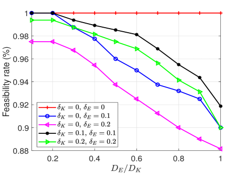
(a) Feasibility rate

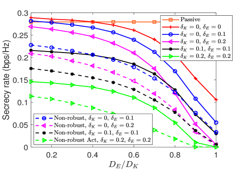
(b) Secrecy rate

Figure 3: Performance versus $D_{E}/D_{K}$ under $N=8$, $M=32$ and $K=5$.

Next, the performance versus the size of the IRS, i.e., $M$, is verified in Fig. 4. Assume that the ED is located at $D_{E}/D_{K}=0.5$. In Fig. 4(a), the feasibility rate decreases rapidly with $M$ when the level of channel uncertainty is high. In Fig. 4(b), the case of $\delta_{K}=\delta_{E}=0$ is regarded as the perfect cascaded CSI case, and its maximum secrecy rate increases with $M$, which is consistent with that of Fig. 6 in [14]. The performance of $\delta_{K}=\delta_{E}=0$ can be used as the performance upper bound of the proposed outage constrained beamforming method. The maximum secrecy rate under small channel uncertainty levels, e.g., $(\delta_{K}=\{0.1,0.2\},\delta_{E}=0)$ or $(\delta_{K}=0,\delta_{E}=0.1)$, also increases with $M$. In addition, it is observed that black lines of $\delta_{E}=0$ are higher than blue lines of $\delta_{K}=0$, which means that the negative impact of cascaded LIL channel error on secrecy rate is smaller than that of the cascaded LIE channel error. Furthermore, when $\delta_{\mathrm{E}}$ increases to $0.1$ or larger, secrecy rate starts to decrease at large $M$. The reason is that increasing $M$ can not only enhance the secrecy rate due to its increased beamforming gain, but also increase the cascaded channel estimation error.

Therefore, at small channel uncertainty level, especially that of the ED, the benefits brought by the increased $M$ outweighs its drawbacks, and vice versa. This observation provides useful guidance to carefully chose the size of the IRS according to the level of the channel uncertainty.

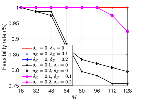
(a) Feasibility rate

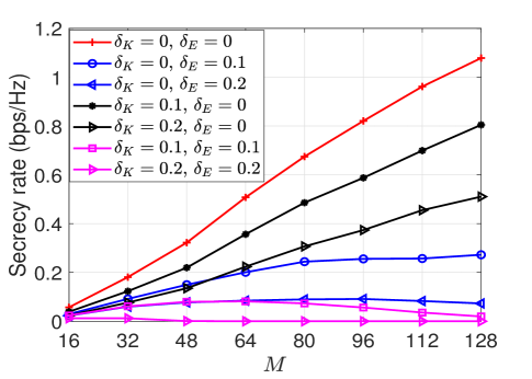
(b) Secrecy rate

Figure 4: Performance versus $M$ under $N=8$ and $K=5$.

V-B Average secrecy rate in ED Model II

This subsection evaluates the performance of the proposed scheme under the passive attack. In order to evaluate the performance of the proposed low complexity algorithm, we consider two benchmark algorithms which are given by: 1) The “SOCP” based scheme, i.e., the CVX is used to solve the SOCP version of Problem (59). 2) The “Random” phase scheme, in which the phases of the reflection elements are randomly generated.

Under the case of $N=8$ and $K=5$, the average secrecy rate versus $M$ is shown in Fig. 5(a). It can be seen that the performance of the proposed algorithm is almost the same as that of the SOCP algorithm, and both of them outperform the scheme with random phases. Moreover, increasing the size of the IRS can significantly increase the average secrecy rate of the system. Accordingly, Fig. 5(b) describes the CPU time required for these three algorithms. The simulation setup is the same as that of Fig. 5(a). It is observed from Fig. 5(b) that the proposed algorthm with closed-form solution requires much less CPU running time than the SOCP scheme. In addition, the CPU running time of the SCOP-based algorithm increases significantly with the size of the IRS, but the proposed algorithm is not sensitive to the size of the IRS. This is because the computational complexity of the SOCP depends on $M$, while that of the closed-form solution does not.

(a) Average secrecy rate

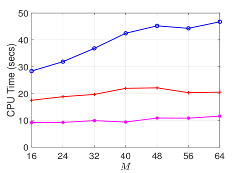
(b) Average CPU time

Figure 5: Performance versus $M$ under $N=8$ and $K=5$.

Finally, Fig. 6 illustrates the performance and the complexity versus the number of users in the case of $M=64$. Again, the proposed algorithm can achieve the same performance of the SOCP-based scheme with less CPU running time. However, the average secrecy rate is saturated when the number of users is greater than 7.

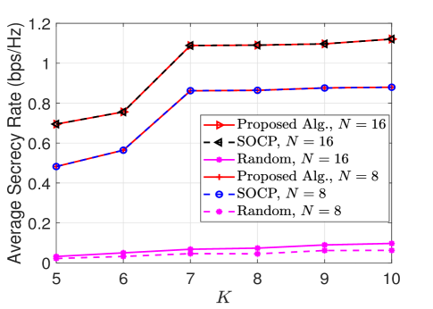
(a) Average secrecy rate

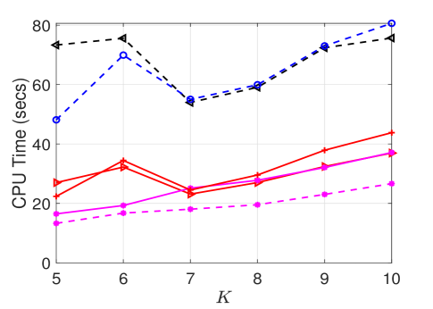
(b) Average CPU time

Figure 6: Performance versus $K$ under $M=64$.

VI Conclusions

In this work, we have proposed a two-phase IRS-aided communication system to realize the secure communication under the active attacks and passive eavesdropping. In order to address the cascaded channel error caused by the active attacks, we maximize the secrecy rate subject to secrecy rate outage probability constraints, which has been tackled by using the Bernstein-Type inequality. For the case of the partial CSI of the ED, average secrecy rate maximization problem was considered, which is addressed by the proposed low-complexity algorithm. It was shown that the negative effect of the ED’s channel error is greater than that of the LU. In addition, the number of elements on the IRS has a negative impact on system performance when the channel error is large. This conclusion provides an engineering insight for the careful selection of the number of elements at the IRS.

Appendix A The proof of Lemma 2

To begin, we introduce the following lemma.

Lemma 8

Let $x\geq 0$ be a positive real number, and consider the function $g_{1}(a,x)=-ax+\ln a+1$, then

$$\ln x^{-1}=\max_{a\geq 0}g_{1}(a,x).$$

By appying Lemma 8, we can construct an upper bound of rate $R_{E}\left(\mathbf{w},\mathbf{e}\right)$ as

$$R_{E}\left(\mathbf{w},\mathbf{e}\right) =\frac{-\ln(1+\left|\mathbf{e}^{\mathrm{H}}\mathbf{H}_{E}\mathbf{w}\right|^{2}/\sigma_{E}^{2})^{-1}}{2\ln 2}$$

$$\overset{\mathrm{(a)}}{=}\frac{-\max_{a_{E}\geq 0}g_{1}(a_{E},1+\left|\mathbf{e}^{\mathrm{H}}\mathbf{H}_{E}\mathbf{w}\right|^{2}/\sigma_{E}^{2})}{2\ln 2}$$

$$=\frac{\min_{a_{E}\geq 0}-g_{1}(a_{E},1+\left|\mathbf{e}^{\mathrm{H}}\mathbf{H}_{E}\mathbf{w}\right|^{2}/\sigma_{E}^{2})}{2\ln 2}$$

$$\leq\frac{-g_{1}(a_{E},1+\left|\mathbf{e}^{\mathrm{H}}\mathbf{H}_{E}\mathbf{w}\right|^{2}/\sigma_{E}^{2})}{2\ln 2},\textrm{for any }a_{E}\geq 0$$

$$=\frac{a_{E}\left|\mathbf{e}^{\mathrm{H}}\mathbf{H}_{E}\mathbf{w}\right|^{2}/\sigma_{E}^{2}+a_{E}-\ln a_{E}-1}{2\ln 2}$$

$$=\widetilde{R}_{E}\left(\mathbf{w},\mathbf{e},a_{E}\right),$$ (67)

where the equality (a) is from Lemma 8.

Hence, the proof is completed.

Appendix B The proof of Lemma 3

To prove Lemma 3, we first introduce the following lemma.

Lemma 9

Let $v$ be a complex number, and consider the function $g_{2}(v,x)=(|x|^{2}+\sigma^{2})|v|^{2}-2\text{Re}\left\{vx\right\}+1$, then

$$\frac{\sigma^{2}}{|x|^{2}+\sigma^{2}}=\min_{v}g_{2}(a,x).$$

By appying Lemma 9, we can construct a lower bound of rate $R_{K}\left(\mathbf{w},\mathbf{e}\right)$ as

$$R_{K}\left(\mathbf{w},\mathbf{e}\right) =\frac{\ln\left(1-\frac{\left|\mathbf{e}^{\mathrm{H}}\mathbf{H}_{K}\mathbf{w}\right|^{2}}{\sigma_{K}^{2}+\left|\mathbf{e}^{\mathrm{H}}\mathbf{H}_{K}\mathbf{w}\right|^{2}}\right)^{-1}}{2\ln 2}$$

$$\overset{\mathrm{(a)}}{=}\frac{\max_{a_{K}\geq 0}g(a_{K},1-\frac{\left|\mathbf{e}^{\mathrm{H}}\mathbf{H}_{K}\mathbf{w}\right|^{2}}{\sigma_{K}^{2}+\left|\mathbf{e}^{\mathrm{H}}\mathbf{H}_{K}\mathbf{w}\right|^{2}})}{2\ln 2}$$

$$\geq\frac{g(a_{K},1-\frac{\left|\mathbf{e}^{\mathrm{H}}\mathbf{H}_{K}\mathbf{w}\right|^{2}}{\sigma_{K}^{2}+\left|\mathbf{e}^{\mathrm{H}}\mathbf{H}_{K}\mathbf{w}\right|^{2}})}{2\ln 2},\textrm{for any }a_{K}\geq 0$$

$$=\frac{-a_{K}\left(\frac{\sigma_{K}^{2}}{\sigma_{K}^{2}+\left|\mathbf{e}^{\mathrm{H}}\mathbf{H}_{K}\mathbf{w}\right|^{2}}\right)+\ln a_{K}+1}{2\ln 2}$$

$$\overset{\mathrm{(b)}}{=}\frac{-a_{K}\left(\min_{v}g_{2}(v,\mathbf{e}^{\mathrm{H}}\mathbf{H}_{K}\mathbf{w})\right)+\ln a_{K}+1}{2\ln 2}$$

$$=\frac{a_{K}\left(\max_{v}-g_{2}(v,\mathbf{e}^{\mathrm{H}}\mathbf{H}_{K}\mathbf{w})\right)+\ln a_{K}+1}{2\ln 2}$$

$$\geq\frac{a_{K}\left(-g_{2}(v,\mathbf{e}^{\mathrm{H}}\mathbf{H}_{K}\mathbf{w})\right)+\ln a_{K}+1}{2\ln 2},\textrm{for any }v\geq 0$$

$$=\frac{1}{2\ln 2}(-a_{K}|v|^{2}|\mathbf{e}^{\mathrm{H}}\mathbf{H}_{K}\mathbf{w}|^{2}-\sigma_{K}^{2}a_{K}|v|^{2}+2a_{K}\text{Re}\left\{v\mathbf{e}^{\mathrm{H}}\mathbf{H}_{K}\mathbf{w}\right\}-a_{K}+\ln a_{K}+1)$$

$$=\widetilde{R}_{K}\left(\mathbf{w},\mathbf{e},a_{K},v\right)$$ (68)

where Equality (a) is from Lemma 8, and Equality (b) is from Lemma 9.

Hence, the proof is completed.

Appendix C The proof of Lemma 7

To begin with, we solve $\mathcal{P}1$: $\mathcal{P}1$ is equivalent to

$$\min\limits_{\mathbf{e}} \thinspace\thinspace\mathbf{e}^{\mathrm{H}}\mathbf{A}_{E}\mathbf{e}$$ (69a)

$$\mathrm{s.t.} (\ref{eq:e-c}),$$ (69b)

$$\mathbf{e}^{\mathrm{H}}\mathbf{A}_{K}\mathbf{e}\geq e^{2\mathcal{R}}-1.$$ (69c)

Step 1: Construct a surrogate problem: Under the MM algorithm framework [27], we have the following lemma.

Lemma 10

[28, 29] Given $\mathbf{A}\succeq\mathbf{A}_{0}$ and $\mathbf{x}$, then quadratic function $\mathbf{x}^{\mathrm{H}}\mathbf{A}_{0}\mathbf{x}$ is majorized by $\mathbf{x}^{\mathrm{H}}\mathbf{A}\mathbf{x}-2\mathrm{Re}\{\mathbf{x}^{(n),\mathrm{H}}(\mathbf{A}-\mathbf{A}_{0})\mathbf{x}\}+\mathbf{x}^{(n),\mathrm{H}}(\mathbf{A}-\mathbf{A}_{0})\mathbf{x}^{(n)}$ at $\mathbf{x}^{(n)}$.

By adopting Lemma 10 and setting $\mathbf{A}=\lambda_{\max}(\mathbf{A}_{E})\mathbf{I}$ for simplicity, the quadratic objective function in (69a) is majorized by

$$2\lambda_{\max}(\mathbf{A}_{E})M -2\mathrm{Re}\{\mathbf{e}^{(n),\mathrm{H}}(\lambda_{\max}(\mathbf{A}_{E})\mathbf{I}-\mathbf{A}_{E})\mathbf{e}\}-\mathbf{e}^{(n),\mathrm{H}}\mathbf{A}_{E}\mathbf{e}^{(n)}$$ (70)

at feasible point $\mathbf{e}^{(n)}$. To deal with the non-convex constraint (69c), we replace $\mathbf{e}^{\mathrm{H}}\mathbf{A}_{K}\mathbf{e}$ with its linear lower bound, resulting in the following equivalent constraint

$$(\ref{eq:r-c1})\Rightarrow 2\mathrm{Re}\{\mathbf{e}^{(n),\mathrm{H}}\mathbf{A}_{K}\mathbf{e}\}\geq e^{2\mathcal{R}}-1+\mathbf{e}^{(n),\mathrm{H}}\mathbf{A}_{K}\mathbf{e}^{(n)}.$$ (71)

Step 2: Closed-form solution :

By omitting the constant, Problem (69) then becomes

$$\max\limits_{\mathbf{e}} \ 2\mathrm{Re}\{\mathbf{e}^{(n),\mathrm{H}}(\lambda_{\max}(\mathbf{A}_{E})\mathbf{I}-\mathbf{A}_{E})\mathbf{e}\},$$ (72a)

s.t. $$\ (\ref{eq:e-c}),(\ref{eq:r-c2}).$$ (72b)

According to [25], we introducing a price mechanism for solving Problem (72), i.e.,

$$\max\limits_{\mathbf{e}} \thinspace\thinspace 2\mathrm{Re}\{\mathbf{e}^{(n),\mathrm{H}}(\lambda_{\max}(\mathbf{A}_{E})\mathbf{I}-\mathbf{A}_{E})\mathbf{e}\}+\varrho_{1}2\mathrm{Re}\{\mathbf{e}^{(n),\mathrm{H}}\mathbf{A}_{K}\mathbf{e}\}$$

$$\mathrm{s.t.}$$   (11d).

where $\varrho_{1}$ is a nonnegative price. Then, the globally optimal solution is given by

$$\mathbf{e}_{1}^{\#}(\varrho_{1}^{opt})=\exp\{\mathrm{j}\arg((\lambda_{\max}(\mathbf{A}_{E})\mathbf{I}-\mathbf{A}_{E}+\varrho_{1}\mathbf{A}_{K})\mathbf{e}^{(n)})\}.$$

The optimal $\varrho_{1}^{opt}$ is determined by using the bisection search method, the detailed information about which can be found in [25].

Then, we solve $\mathcal{P}2$: $\mathcal{P}2$ is equivalent to

$$\max\limits_{\mathbf{e}} \ \frac{1+\mathbf{e}^{\mathrm{H}}\mathbf{A}_{K}\mathbf{e}}{1+\mathbf{e}^{\mathrm{H}}\mathbf{A}_{E}\mathbf{e}},$$ (73a)

$$\mathrm{s.t.} \ (\ref{eq:e-c}),$$ (73b)

$$\ \mathbf{e}^{\mathrm{H}}\mathbf{A}_{K}\mathbf{e}\leq e^{2\mathcal{R}}-1.$$ (73c)

Step 1: Construct a surrogate problem: Under the MM algorithm framework, we construct a linear lower bound of the objective funcion in (73a) as

$$\frac{1+\mathbf{e}^{\mathrm{H}}\mathbf{A}_{K}\mathbf{e}}{1+\mathbf{e}^{\mathrm{H}}\mathbf{A}_{E}\mathbf{e}} \overset{\mathrm{(a)}}{\geq}\frac{2\mathrm{Re}\{1+d_{K}\}}{1+d_{E}^{(n)}}-\frac{1+d_{K}^{(n)}}{(1+d_{E}^{(n)})^{2}}\left(1+\mathbf{e}^{\mathrm{H}}\mathbf{A}_{E}\mathbf{e}\right)$$

$$\overset{\mathrm{(b)}}{\geq}\frac{2\mathrm{Re}\{1+d_{K}\}}{1+d_{E}^{(n)}}-\frac{1+d_{K}^{(n)}}{(1+d_{E}^{(n)})^{2}}-\frac{1+d_{K}^{(n)}}{(1+d_{E}^{(n)})^{2}}(2\lambda_{\max}(\mathbf{A}_{E})M$$

$$\ -2\mathrm{Re}\{\mathbf{e}^{(n),\mathrm{H}}(\lambda_{\max}(\mathbf{A}_{E})\mathbf{I}-\mathbf{A}_{E})\mathbf{e}\}-d_{E}^{(n)})$$

$$=2\mathrm{Re}\{\mathbf{c}^{\mathrm{H}}\mathbf{e}\}+\mathrm{const},$$

where $d_{K}=\mathbf{e}^{(n),\mathrm{H}}\mathbf{A}_{K}\mathbf{e}$. $\{d_{K}^{(n)},d_{E}^{(n)},\mathbf{c}\}$ are defined in Lemma 7. Inequality (a) is due to Lemma 1, and inequality (b) is from Lemma 10. By using Lemma 10 again, the convex constraint (73c) can be replaced by an easy-to-solve form as

$$(\ref{eq:r-c2-1})\Rightarrow 2\mathrm{Re}\{\mathbf{e}^{(n),\mathrm{H}}(\lambda_{\max}(\mathbf{A}_{K})\mathbf{I}-\mathbf{A}_{K})\mathbf{e}\}$$

$$\geq-2\lambda_{\max}(\mathbf{A}_{K})M-e^{2\mathcal{R}}+1-\mathbf{e}^{(n),\mathrm{H}}\mathbf{A}_{K}\mathbf{e}^{(n)}.$$ (74)

Step 2: Closed-form solution: By omitting the constant, Problem (73) is then equivalent to

$$\max\limits_{\mathbf{e}} \thinspace\thinspace 2\mathrm{Re}\{\mathbf{c}^{\mathrm{H}}\mathbf{e}\},$$ (75a)

$$\mathrm{s.t.} \ (\ref{eq:e-c}),(\ref{eq:ff-1}).$$ (75b)

By using the price mechanism, Problem (73) is reformulated as

$$\max\limits_{\mathbf{e}} \thinspace\thinspace 2\mathrm{Re}\{\mathbf{c}^{\mathrm{H}}\mathbf{e}\}+\varrho_{2}2\mathrm{Re}\{\mathbf{e}^{(n),\mathrm{H}}(\lambda_{\max}(\mathbf{A}_{K})\mathbf{I}-\mathbf{A}_{K})\mathbf{e}\}$$

$$\mathrm{s.t.} (\ref{eq:e-c}).$$

where $\varrho_{2}$ is a nonnegative price. The globally optimal solution is given by $\mathbf{e}_{2}^{\#}(\varrho_{2}^{opt})=\exp\{\mathrm{j}\arg(\mathbf{c}+\varrho_{2}(\lambda_{\max}(\mathbf{A}_{K})\mathbf{I}-\mathbf{A}_{K})\mathbf{e}^{(n)})\}$ where the optimal $\varrho_{2}^{opt}$ is determined by using the bisection search method.

Hence, the proof is completed.

References

• [1] W. Diffie and M. E. Hellman, “New directions in cryptography,” IEEE Trans. Inf. Theory, vol. IT-22, no. 6, pp. 644–654, Nov. 1976.
• [2] A. D. Wyner, “The wire-tap channel,” Bell Syst. Tech. J., vol. 54, no. 8, pp. 1355–1387, Oct. 1975.
• [3] E. Basar, M. Di Renzo, J. De Rosny, M. Debbah, M. Alouini, and R. Zhang, “Wireless communications through reconfigurable intelligent surfaces,” IEEE Access, vol. 7, pp. 116 753–116 773, 2019.
• [4] K. Ntontin, M. Di Renzo, J. Song et al., “Reconfigurable intelligent surfaces vs. relaying: Differences, similarities, and performance comparison,” 2019. [Online]. Available: https://arxiv.org/abs/1908.08747
• [5] K.-K. Wong, K.-F. Tong, Z. Chu, and Y. Zhang, “A vision to smart radio environment: Surface wave communication superhighways,” 2020. [Online]. Available: https://arxiv.org/abs/2005.14082
• [6] H. Shen, W. Xu, S. Gong, Z. He, and C. Zhao, “Secrecy rate maximization for intelligent reflecting surface assisted multi-antenna communications,” IEEE Commun. Lett., vol. 23, no. 9, pp. 1488–1492, Sept. 2019.
• [7] S. Hong, C. Pan, H. Ren, K. Wang, and A. Nallanathan, “Artificial-noise-aided secure mimo wireless communications via intelligent reflecting surface,” IEEE Trans. Commun., vol. 68, no. 12, pp. 7851–7866, Dec. 2020.
• [8] X. Guan, Q. Wu, and R. Zhang, “Intelligent reflecting surface assisted secrecy communication: Is artificial noise helpful or not?” 2020. [Online]. Available: https://arxiv.org/abs/1907.12839
• [9] X. Yu, D. Xu, Y. Sun, D. W. K. Ng, and R. Schober, “Robust and secure wireless communications via intelligent reflecting surfaces,” 2020. [Online]. Available: https://arxiv.org/abs/1912.01497
• [10] S. Hong, C. Pan, H. Ren, K. Wang, K. K. Chai, and A. Nallanathan, “Robust transmission design for intelligent reflecting surface aided secure communication systems with imperfect cascaded CSI,” IEEE Trans. Wireless Commun., early access, pp. 1–1, 2020.
• [11] D. Kapetanovic, G. Zheng, and F. Rusek, “Physical layer security for massive MIMO: An overview on passive eavesdropping and active attacks,” IEEE Commun. Mag., vol. 53, no. 6, pp. 21–27, Jun. 2015.
• [12] Y. Wu, A. Khisti, C. Xiao, G. Caire, K. Wong, and X. Gao, “A survey of physical layer security techniques for 5g wireless networks and challenges ahead,” IEEE J. Sel. Areas Commun., vol. 36, no. 4, pp. 679–695, Apr. 2018.
• [13] G. Zhou, C. Pan, H. Ren, K. Wang, and A. Nallanathan, “A framework of robust transmission design for IRS-aided MISO communications with imperfect cascaded channels,” IEEE Trans. Signal Process., vol. 68, pp. 5092–5106, Aug. 2020.
• [14] ——, “Intelligent reflecting surface aided multigroup multicast MISO communication systems,” IEEE Trans. Signal Process., pp. 1–1, 2020.
• [15] S. Wang, M. Wen, M. Xia, R. Wang, Q. Hao, and Y.-C. Wu.
• [16] S. Boyd and L. Vandenberghe, Convex optimization.   Cambridge Univ. Press, 2004.
• [17] I. Bechar, “A bernstein-type inequality for stochastic processes of quadratic forms of Gaussian variables,” 2009. [Online]. Available: https://arxiv.org/abs/0909.3595
• [18] M. Grant and S. Boyd, “CVX: MATLAB software for disciplined convex programming,” Version 2.1. [Online] http://cvxr.com/cvx, Dec. 2018.
• [19] G. Zhou, C. Pan, H. Ren et al., “Robust beamforming design for intelligent reflecting surface aided MISO communication systems,” IEEE Wireless Commun. Lett., vol. 9, no. 10, pp. 1658–1662, Oct. 2020.
• [20] T. Lipp and S. Boyd, “Variations and extension of the convex-concave procedure,” Optim. Eng., vol. 17, no. 2, pp. 263–287, 2016. [Online]. Available: https://doi.org/10.1007/s11081-015-9294-x
• [21] A. Chaman, J. Wang, J. Sun, H. Hassanieh, and R. R. Choudhury, “Ghostbuster: Detecting the presence of hidden eavesdroppers,” Proc. ACM Mobicom, pp. 337–351.
• [22] A. Mukherjee, “Physical-layer security in the internet of things: Sensing and communication confidentiality under resource constraints,” Proc. IEEE, vol. 103, no. 10, pp. 1747–1761, 2015.
• [23] L. Mucchi, L. Ronga, X. Zhou, K. Huang, Y. Chen, and R. Wang, “A new metric for measuring the security of an environment: The secrecy pressure,” IEEE Trans. Wireless Commun., vol. 16, no. 5, pp. 3416–3430, 2017.
• [24] Ö. Özdogan, E. Björnson, and E. G. Larsson, “Massive MIMO with spatially correlated rician fading channels,” IEEE Trans. Commun., vol. 67, no. 5, pp. 3234–3250, May 2019.
• [25] C. Pan, H. Ren, K. Wang, M. Elkashlan, A. Nallanathan, J. Wang, and L. Hanzo, “Intelligent reflecting surface aided MIMO broadcasting for simultaneous wireless information and power transfer,” IEEE J. Sel. Areas Commun., 2020.
• [26] B. R. Marks and G. P. Wright, “A general inner approximation algorithm for nonconvex mathematical programs,” Operation Research, vol. 26, no. 4, Jul. 1978.
• [27] Y. Sun, P. Babu, and D. P. Palomar, “Majorization-minimization algorithms in signal processing, communications, and machine learning,” IEEE Trans. Signal Process., vol. 65, no. 3, pp. 794–816, Feb. 2017.
• [28] J. Song, P. Babu, and D. P. Palomar, “Optimization methods for designing sequences with low autocorrelation sidelobes,” IEEE Trans. Signal Process., vol. 63, no. 15, pp. 3998–4009, Aug. 2015.
• [29] C. Pan, H. Ren, K. Wang, W. Xu, M. Elkashlan, A. Nallanathan, and L. Hanzo, “Multicell MIMO communications relying on intelligent reflecting surfaces,” IEEE Trans. Wireless Commun., pp. 1–1, 2020.