Electromagnetic instabilities of low-beta alpha/proton beams in space plasmas

Abstract

Relative drifts between different species or particle populations are characteristic to solar plasma outflows, e.g., in the fast streams of the solar winds, coronal mass ejections and interplanetary shocks. This paper characterizes the dispersion and stability of the low-beta alpha/proton drifts in the absence of any intrinsic thermal anisotropies, which are usually invoked in order to stimulate various instabilities. The dispersion relations derived here describe the full spectrum of instabilities and their variations with the angle of propagation and plasma parameters. The results unveil a potential competition between instabilities of the electromagnetic proton cyclotron and alpha cyclotron modes. For conditions specific to a low-beta solar wind, e.g., at low heliocentric distances in the outer corona, the instability operates on the alpha cyclotron branch. The growth rates of the alpha cyclotron mode are systematically stimulated by the (parallel) plasma beta and/or the alpha-proton temperature ratio. One can therefore expect that this instability develops even in the absence of temperature anisotropies, with potential to contribute to a self-consistent regulation of the observed drift of alpha particles.

1 Introduction

Plasma outflows released by the Sun in interplanetary space consist mainly of electrons, protons and minor ions, among which the alpha particles are dominant with an average abundance of about 5% of the total number density of ions. Owing to their mass density, typically 20% of the total ion mass density, alpha-ions may have important implications in the solar wind dynamics (Robbins et al., 1970; Marsch, 2006; Kasper et al., 2007; Maruca et al., 2012; Maneva et al., 2014). The in-situ measurements in the fast wind and regions not too distant from the Sun, i.e., $\lesssim 1$ AU, have revealed alpha particle streams faster than the protons, with relative speeds of the order of local Alfvén speed (Asbridge et al., 1976; Marsch et al., 1982; Neugebauer, 1981), and kinetic temperatures in general higher than proton temperature (Kohl et al., 1998). This preferential energization of heavier ions in collision-poor plasmas is attributed to the interaction with plasma waves, via Landau or cyclotron resonances (Marsch, 2006), and is supported by observations (Marsch, 1991; von Steiger et al., 1995).

The observed velocity distributions display strong deviations from thermal equilibrium, often with a dual structure combining a proton core and a drifting alpha population called alpha beam (Marsch et al., 1982). Non-thermal features of the observed ion distributions are sources of free energy that can locally generate instabilities and enhanced wave fluctuations (Gary, 1993). In our case, beaming alpha populations may destabilize the plasma system via excitations associated with the Alfvén/ion cyclotron waves and the fast magnetosonic/whistler modes (Revathy, 1978; Gary et al., 2000b; Li and Habbal, 1999). In turn, these fluctuations regulate the ion VDFs through the same wave-particle interactions, which determine a diffusion in velocity space and a thermalisation and relaxation of the alpha beam (Marsch and Livi, 1987; Gary et al., 2000a). The observations confirm that the alphas are heated in perpendicular direction and cool more slowly than what would be expected from adiabatic expansion (Reisenfeld et al., 2001; Stansby et al., 2019).

The investigations of alpha-ion beams have initially concluded that high plasma beta conditions, e.g., $\beta\geqslant 1$, more typical to large heliospheric distances ($\geqslant 1$ AU), can be favorable to magnetosonic instabilities, with a maximum growth for propagation parallel to the interplanetary magnetic field (Gary et al., 2000b, a). Later it was shown that magnetosonic instabilities were stimulated by an internal anisotropic temperature $T_{\perp}/T_{\parallel}<1$ of protons or alpha particles ($\parallel,\perp$ being directions with respect to the magnetic field), while isotropic beams, with, e.g., $T_{\alpha,\perp}/T_{\alpha,\parallel}\simeq 1$, may drive another instability of the parallel-propagating Alfvén/ion-cyclotron waves (Verscharen et al., 2013). The ion-beam instabilities are also highly dependent on the plasma beta, which decreases towards the Sun and in the outer corona ($\sim 0.3$ AU) becomes $\beta_{p,\alpha}=8\pi n_{p,\alpha}T_{p,\alpha}/B_{0}^{2}<1$ for both the protons (subscript $p$) or alpha particles (subscript $\alpha$) (Marsch et al., 1982). Here, $n_{p,\alpha}$ denote proton/alpha number densities, $T_{p,\alpha}$ their respective temperatures (in the unit of energy), and $B_{0}$ denotes the ambient magnetic field intensity. The low-beta alpha/proton beams appear to be more susceptible to Alfvénic instabilities, but again, it is not clear if these instabilities are driven by the alpha/proton drift or by the anisotropic temperature $T_{\perp}/T_{\parallel}>1$, as such a condition is always assumed for protons or alpha particles in the literature (Li and Habbal, 1999; Gomberoff and Valdivia, 2003). In the outer corona an excess of temperature (kinetic energy) in perpendicular direction may be associated only to the proton core, while suprathermal populations including proton halo or beams of protons and alpha particles rather show an opposite, relatively small anisotropy $T_{\perp}/T_{\parallel}\lesssim 1$ (Marsch et al., 1982; Marsch, 2006).

In order to complete the picture and provide a clear basic characterization of these instabilities, in the present paper we reduce the complexity of the low-beta beaming plasmas, and investigate alpha/proton drifting populations with isotropic temperatures $T_{\perp}/T_{\parallel}=1$. The dispersion and stability properties of the plasma system are derived on the basis of a general kinetic approach, which cover the full spectrum of wave-frequencies, wave-numbers and angles of propagation with respect to the magnetic field. The organization of our paper is the following: In section 2, we derive the general dispersion relation for the electromagnetic modes propagating at an arbitrary angle. Growth rates of the unstable solutions are obtained for standard representations of the particle velocity distribution as drifting-Maxwellians in section 3. The unstable solutions are discussed by numerical means in Section 4, providing also an analysis of their variation with the main plasma parameters. Section 5 summarizes our present results.

2 Dispersion Relation

In a collision-poor plasma the general linear dispersion relation for electromagnetic modes propagating at an arbitrary angle $\theta$ with respect to the uniform background magnetic field ($\bm{B}_{0}=B_{0}\hat{\bm{z}}$) is given by

$$0=\det\left|\epsilon_{ij}(\bm{k},\omega)-\frac{c^{2}k^{2}}{\omega^{2}}\left(\delta_{ij}-\frac{k_{i}k_{j}}{k^{2}}\right)\right|,$$ (1)

with a dielectric tensor defined by

$$\epsilon_{ij} = \delta_{ij}+\sum_{a}\frac{\omega_{pa}^{2}}{\omega^{2}}\int d{\bf v}\left[v_{\parallel}\left(\frac{\partial}{\partial v_{\parallel}}-\frac{v_{\parallel}}{v_{\perp}}\frac{\partial}{\partial v_{\parallel}}\right)b_{j}f_{a}\right.$$ (2)

$$+\sum_{n=-\infty}^{\infty}\frac{V_{i}V_{j}^{*}}{\omega-n\Omega_{a}-k_{\parallel}v_{\parallel}}$$

$$\left.\times\left(\frac{n\Omega_{a}}{v_{\perp}}\frac{\partial}{\partial v_{\perp}}+k_{\parallel}\frac{\partial}{\partial v_{\parallel}}\right)f_{a}\right],$$

where $\omega$ is the wave frequency, $b_{i}=\bm{B}_{0}/B_{0}=\hat{\bm{z}}$ is the unit vector along the direction of ambient magnetic field vector, $f_{a}(v_{\perp},v_{\parallel})$ is the velocity distribution function for particle species labeled $a$ ($a=e,p,\alpha$, etc., for electrons, protons, alpha particles, etc.), $\omega_{pa}=~{}\sqrt{4\pi n_{a}e^{2}/m_{a}}$ and $\Omega_{a}=e_{a}B_{0}/m_{a}$ are the plasma and cyclotron frequencies for species $a$, and

$$V_{i} = \left(v_{\perp}\frac{nJ_{n}(b)}{b},\mbox{ }-iv_{\perp}J^{\prime}_{n}(b),\mbox{ }v_{\parallel}J_{n}(b)\right)_{i},$$

$$b = \frac{k_{\perp}v_{\perp}}{\Omega_{a}}.$$ (3)

Here, $J_{n}$ is a Bessel function of the first kind, of order $n$, with argument $b$. In the above, $e$, $n_{a}$, $m_{a}$, and $c$ stand for unit electric charge, ambient density for plasma particle species $a$, their mass, and the speed of light in vacuo, respectively.

In the present analysis we adopt the cold plasma approximation for the real frequency, combined with warm plasma growth/damping rate expression in the context of weak growth/damping formula, or equivalent, the dissipative instability formalism. The weak growth or dissipative instability theory is also known as the weak kinetic instability theory, as opposed to the reactive or fluid instability theory. We take the general cold plasma dielectric tensor elements given in component form by

$$\epsilon_{xx} =1-\frac{\omega_{pe}^{2}}{\omega^{2}-\Omega_{e}^{2}}-\sum_{a}\frac{\omega_{pa}^{2}}{\omega^{2}-\Omega_{a}^{2}}=\epsilon_{yy},$$

$$\epsilon_{xy} =-i\,\frac{\Omega_{e}}{\omega}\frac{\omega_{pe}^{2}}{\omega^{2}-\Omega_{e}^{2}}+i\sum_{a}\frac{\Omega_{a}}{\omega}\frac{\omega_{pa}^{2}}{\omega^{2}-\Omega_{a}^{2}}=-\epsilon_{yx},$$

$$\epsilon_{xz} =\epsilon_{zx}=0=\epsilon_{yz}=\epsilon_{zy},$$

$$\epsilon_{zz} =1-\frac{\omega_{pe}^{2}}{\omega^{2}}-\sum_{a}\frac{\omega_{pa}^{2}}{\omega^{2}},$$ (4)

and further approximate the situation by considering two species ions, namely, protons and alpha particles, and ignore the displacement current, that is, the unity on the right-hand side of Eq. (4), which is valid for low frequency waves. We also assume $\omega^{2}\ll\Omega_{e}^{2}$, in order to simplify the dielectric tensor elements,

$$\epsilon_{xx} \approx-\frac{\omega_{pp}^{2}}{\omega^{2}-\Omega_{p}^{2}}-\frac{\omega_{p\alpha}^{2}}{\omega^{2}-\Omega_{\alpha}^{2}},$$

$$\epsilon_{xy} =i\,\frac{\omega_{pp}^{2}}{\omega\Omega_{p}}\left(\frac{n_{0}}{n_{p}}+\frac{\Omega_{p}^{2}}{\omega^{2}-\Omega_{p}^{2}}\right)+i\,\frac{\Omega_{\alpha}}{\omega}\frac{\omega_{p\alpha}^{2}}{\omega^{2}-\Omega_{\alpha}^{2}},$$

$$\epsilon_{zz} =-\frac{m_{p}}{m_{e}}\frac{n_{0}}{n_{p}}\frac{\omega_{pp}^{2}}{\omega^{2}},$$ (5)

where $\Omega_{p}=eB_{0}/(m_{p}c)$, $\Omega_{\alpha}=\Omega_{p}/2$, $\omega_{pp}^{2}=4\pi n_{p}e^{2}/m_{p}$, $\omega_{pe}^{2}=m_{p}n_{0}\omega_{pp}^{2}/(m_{e}n_{p})$, and $\omega_{p\alpha}^{2}=(n_{\alpha}/n_{p})\omega_{pp}^{2}$. Note that in $\epsilon_{zz}$ the other ion terms can be neglected compared to $m_{p}/m_{e}\gg 1$.

Substituing the dielectric tensor elements (5) to the dispersion relation (1), it can be shown that the linear dispersion relation is given in dimensionless form by

$$q^{2}=\frac{sx}{(1+\mu^{2})x\mp\sigma\sqrt{(1+\mu^{2})^{2}x^{2}+st\mu^{2}}},$$ (6)

where

$$q=\frac{ck}{\omega_{pp}},\quad x=\frac{\omega}{\Omega_{p}},\quad\mu=\cos\theta,\quad\delta=\frac{n_{\alpha}}{n_{p}},$$ (7)

are dimensionless wave number, frequency, cosine of the wave propagation angle, and the alpha-to-proton density ration, and other quantities are defined by

$$s = \frac{2(xQ_{-}+\delta P_{-}Q_{+})(xQ_{+}+\delta P_{+}Q_{-})}{D},$$

$$\sigma = \frac{|D|}{D},\quad D=Q_{+}Q_{-}+\delta P_{+}P_{-},$$

$$t = \frac{2P_{+}P_{-}Q_{+}Q_{-}}{D},$$

$$P_{\pm} = x\pm 1,\qquad Q_{\pm}=x\pm\tfrac{1}{2}.$$ (8)

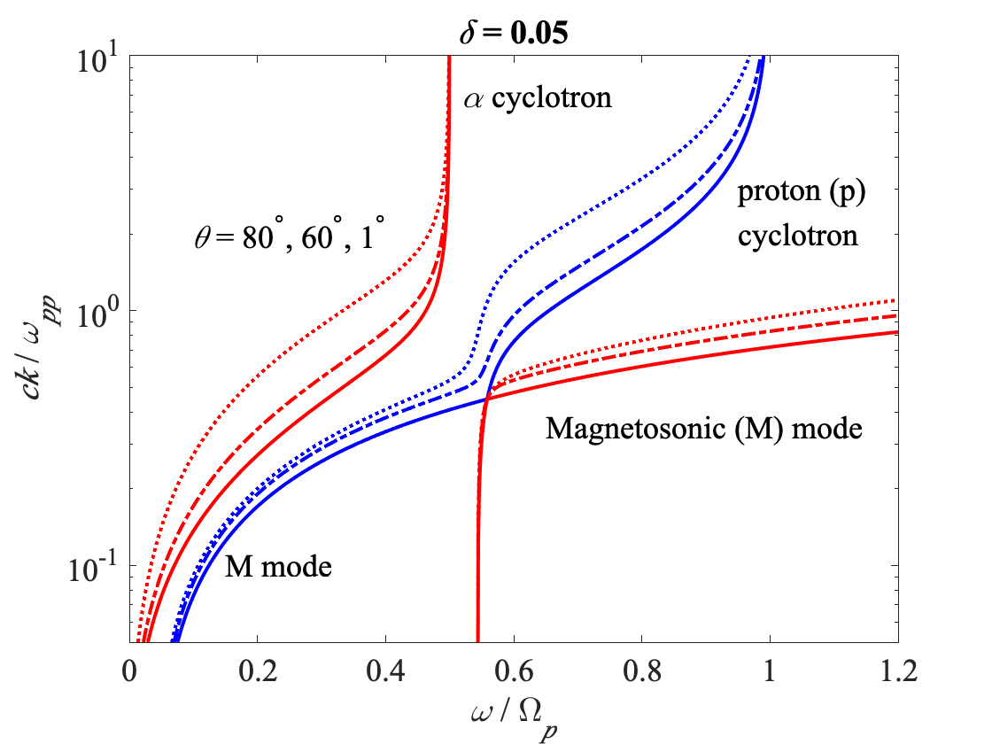
Fig. 1 : Dispersion relation plotted as $q^{2}=c^{2}k^{2}/\omega_{pp}^{2}$ versus $x=\omega/\Omega_{p}$ curves for three different values of $\theta$ corresponding to $1^{\circ}$ (solid line), $60^{\circ}$ (dash-dotted), and $\theta=80^{\circ}$ (dotted).

Figure 1 plots $q$ versus $x$ for three values of $\theta$ corresponding to $1^{\circ}$, $60^{\circ}$, and $80^{\circ}$. The dispersion curves show that they are composed of three distinct branches. The first branch (topmost, color coded in red) denotes the low frequency mode that begins as Alfvén wave for low frequency ($\omega\ll\Omega_{p}$), but gradually turns into the resonant mode (where $k\to\infty$) at the alpha cyclotron frequency, $\omega=\Omega_{\alpha}=\Omega_{p}/2$. For quasi parallel propagation angle ($\theta\to 0$), this branch is left-hand circularly polarized. The second brach (color coded in blue for $\omega<\Omega_{p}$) starts off in low frequency regime ($\omega\ll\Omega_{p}$) as fast/magnetosonic mode, and this mode is right-hand circularly polarized for quasi parallel angle of propagation. For nonzero $\theta$, this mode switches over to the proton cyclotron mode, which becomes resonant ($k\to\infty$) at the proton cyclotron frequency ($\omega=\Omega_{p}$). The switchover takes place in the vicinity of the alpha cyclotron frequency. A third brach that begins as the alpha cyclotron mode turns into the fast/magnetosonic mode above $\Omega_{\alpha}$ and beyond. The third branch is plotted with red color. In general, modes designated with red color corresponds to the lower sign in the dispersion relation (6), while the blue curves belong to the upper sign.

In the growth rate calculation to be discussed subsequently, we will denote instabilities operative on the topmost branch as the “alpha cyclotron” instability, while instabilities operative on the middle, blue-colored mode will be designated as the “proton cyclotron” instability. It turns out that the third, bottommost curve – that is, the fast/magnetosonic mode – remains stable.

3 Growth Rate

Assuming weak growth/damping rate ($|\gamma|\ll\omega$), and following the standard method of derivation (Melrose, 1986) we obtain an explicit expression for the growth/damping rate,

$$\gamma = \sum_{a}\frac{\pi\omega_{pa}^{2}}{\left[1-|{\bf e}({\bf k})\cdot\hat{\bf k}|^{2}\right]\left[\partial(\omega^{2}N^{2})/\partial\omega\right]}$$ (9)

$$\times\int d{\bf v}\sum_{n=-\infty}^{\infty}\left|{\bf e}({\bf k})\cdot{\bf V}\right|^{2}\delta(\omega-n\Omega_{a}-k_{\parallel}v_{\parallel})$$

$$\times\left(\frac{n\Omega_{a}}{v_{\perp}}\frac{\partial}{\partial v_{\perp}}+k_{\parallel}\frac{\partial}{\partial v_{\parallel}}\right)f_{a}\left(v_{\perp},v_{\parallel}\right),$$

where $N=ck/\omega$ is the index of refraction, ${\bf V}$ is defined in Eq. (3), and ${\bf e}$ represents the unit electric field vector, which is discussed in Appendix A. Making use of the dispersion relation (6) one may also compute $\partial(\omega^{2}N^{2})/\partial\omega$ explicitly, which is given in Appendix B. In Eq. (9) $f_{a}=f_{a}(v_{\perp}^{2},v_{\parallel})$ represents the velocity distribution function for ion species labeled $a$. The following is the resulting explicit expression for the growth/damping rate after taking into account the dispersive wave properties associated with the low frequency modes:

$$\frac{\gamma}{\Omega_{p}} = \sum_{a=p,\alpha}\frac{n_{a}}{n_{p}}\frac{m_{p}}{m_{a}}\frac{2\pi^{2}}{(1+M^{2}x^{2}\mu^{2})R}\int_{0}^{\infty}dv_{\perp}v_{\perp}^{3}$$

$$\times\sum_{n=-\infty}^{\infty}\left|M^{2}x^{2}\frac{n^{2}J_{n}^{2}}{b^{2}}+(J^{\prime}_{n})^{2}-2Mx\frac{nJ_{n}J^{\prime}_{n}}{b}\right|$$

$$\times\left(\frac{n\Omega_{a}}{kv_{\perp}\mu}\frac{\partial f_{a}(v_{\perp}^{2},v_{r})}{\partial v_{\perp}}+\frac{\partial f_{a}(v_{\perp}^{2},v_{r})}{\partial v_{r}}\right),$$

$$v_{r} = \frac{\omega-n\Omega_{a}}{k\mu},$$ (10)

where the argument of the Bessel function $b=k_{\perp}v_{\perp}/\Omega_{a}$ applies for proton ($a=p$) and alpha particles ($a=\alpha$), and $M$ and $R$ are defined in Eqs. (A5) and (B2), respectively.

For drifting Maxwellian distributed plasmas we replace the arbitrary distribution function $f_{a}$ in the growth rate expression (3) by

$$f_{a}(v_{\perp},v_{\parallel})=\frac{1}{\pi^{3/2}v_{Ta}^{3}}\exp\left(-\frac{v_{\perp}^{2}}{v_{Ta}^{2}}-\frac{(v_{\parallel}-V_{a})^{2}}{v_{Ta}^{2}}\right),$$ (11)

where $v_{Ta}=(2T_{a}/m_{a})^{1/2}$ stands for thermal speed, and $V_{a}$ represents the average drift speed. After some straightforward mathematical manipulations it can be shown that the growth rate expression reduces to

$$\frac{\gamma}{\Omega_{p}} = -\sum_{a}\frac{n_{a}}{n_{p}}\frac{m_{p}}{m_{a}}\frac{\pi^{1/2}}{(1+M^{2}\mu^{2})R}\sum_{n=-\infty}^{\infty}$$ (12)

$$\times\biggl{(}\frac{n(1+M^{2}x^{2})}{2}\,[I_{n-1}(\lambda_{a})-I_{n+1}(\lambda_{a})]e^{-\lambda_{a}}$$

$$+(Mnx+\lambda_{a})\,[2I_{n}(\lambda_{a})-I_{n-1}(\lambda_{a})$$

$$-I_{n+1}(\lambda_{a})]e^{-\lambda_{a}}\biggr{)}\xi_{a}\exp\left[-(\zeta_{n}^{a})^{2}\right],$$

where $I_{n}$ is the modified Bessel function of the first kind of order $n$, and

$$\xi_{a}=\frac{\omega-kV_{a}\mu}{kv_{Ta}\mu},$$

$$\zeta_{n}^{a}=\frac{\omega-n\Omega_{a}-kV_{a}\mu}{kv_{Ta}\mu},$$

$$\lambda_{a}=\frac{k^{2}v_{Ta}^{2}(1-\mu^{2})}{2\Omega_{a}^{2}}.$$ (13)

4 Numerical Analysis

The growth rate of low frequency modes is a function of frequency $\omega$ and angle of propagation $\theta$. It also depends implicitly on alpha-proton number density ratio $n_{\alpha}/n_{p}$, alpha particle drift velocity $V_{\alpha}$ (we assume zero drift for the protons, $V_{p}=0$), plasma beta parameters $\beta_{p}$ and $\beta_{\alpha}$, where $\beta_{p}=8\pi n_{p}T_{p}/B_{0}^{2}$ and $\beta_{\alpha}=8\pi n_{\alpha}T_{\alpha}/B_{0}^{2}$, respectively. In the fast solar wind alpha particles possess an average density of 5% of the total number density and are drifting with respect to the protons with a typical speed on the order of local Alfvén speed, $V_{\alpha}=v_{A}$ (Marsch et al., 1982; Reisenfeld et al., 2001). Consequently, in the present analysis, for alpha-proton relative number density we consider $n_{\alpha}/n_{p}=0.05$, and for alpha drift velocity, we fix the value at $V_{\alpha}=v_{A}$. For low corona the beta values are relatively low. We thus consider low value of $\beta_{\alpha}=0.01$ and a slightly higher proton beta of $\beta_{p}=2\beta_{\alpha}$, as an example. Note that while $\beta_{\alpha}$ and $\beta_{p}$ are comparable, this actually represent much high alpha particle temperature, since the alpha particle number density is much lower. This is consistent with observation.

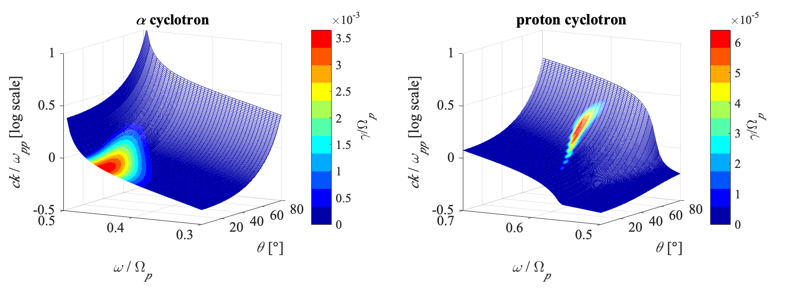
Fig. 2 : Dispersion surfaces corresponding to alpha cyclotron modes [left], and proton cyclotron mode, which includes the magnetosonic mode branch [right]. The color-coded growth rates for each mode is shown, for $n_{\alpha}/n_{p}=0.05$, $T_{\alpha}/T_{p}=2$, and $\beta_{\alpha}=0.01$. Note that the alpha cyclotron instability is an order of magnitude higher than that for the proton cyclotron instability.

Figure 2 displays on the left, the dispersion surface or manifold, corresponding to Alfvén-alpha cyclotron mode, while the right-hand panel plots the dispersion surface, depicting the proton cyclotron branch (which also includes fast/magnetosonic mode brach in the lower frequency regime). Vertical axis represents normalized wave number, $q=ck/\omega_{pp}$, while the two horizontal axes denote normalized (real) frequency $x=\omega/\Omega_{p}$, and wave propagation angle $\theta$, respectively. We indicate the region of wave growth on each surface as well as the magnitude by color scheme. As indicated by color bars, however, it is apparent that the alpha cyclotron instability growth rate is almost an order of magnitude higher than that of proton cyclotron branch. The instability for both branches take place over narrow bands of frequencies and along extended domains of propagation angles. However, only the most unstable alpha cyclotron modes take place along quasi parallel direction, while the peaking growth rates of the proton cyclotron instability peak appear at oblique angles.

In Figure 3 we plot the maximum growth rate for the unstable alpha cyclotron modes, which was determined by surveying the entire frequency and angle space for a given set of input parameters $\beta_{p}$ and $\beta_{\alpha}$. We have then systematically varied both $\beta_{p}$ and $\beta_{\alpha}$, for fixed $\delta=0.05$ and $V_{\alpha}=v_{A}$, until we covered the two dimensional parameter space $(\beta_{p},\beta_{\alpha})$. Figure 3 shows that the alpha cyclotron beam instability becomes more unstable as $\beta_{\alpha}$ decreases, for fixed value of $\beta_{p}$. Of course, one cannot indefinitely decrease $\beta_{\alpha}$, since the present weak growth/damping rate formalism assumes that the distribution function has a relatively mild of velocity space gradient, $\partial f_{\alpha}/\partial v_{\perp}$ and $\partial f_{\alpha}/\partial v_{\parallel}$. For very low $\beta_{\alpha}$ values, the distribution will have a sufficiently high velocity derivative so that the assumption of weak growth rate is violated. Such a caveat notwithstanding, it is interesting to note that the beam-driven alpha cyclotron instability becomes more unstable for lower beta values for alpha particles. Figure 3 shows that the instability is suppressed as the proton beta (or, equivalently, proton temperature) increases.

Figure 4 exhibits the maximum growth rate for proton cyclotron instability in the same format as Fig. 3. Conditions relevant for a low-beta solar wind are in general confined around the solid blue line that corresponds to the sample case assumed in Figure 2. Note that the maximum growth rate is lower in magnitude than that of the alpha cyclotron instability by an order of magnitude in an overall sense. It is interesting to note that the maximum proton cyclotron beam instability has a peak value around $\beta_{\alpha}\sim 10^{-1}$, but for both higher and lower $\beta_{\alpha}$, the maximum growth rate decreases. This behavior is in contrast to that of the alpha cyclotron instability, where the alpha cyclotron instability monotonically increases in magnitude of the maximum growth rate as $\beta_{\alpha}$ is decreased (until, presumably, the assumption of weak growth rate is eventually violated). Note that the proton cyclotron instability is also suppressed by increasing proton beta, which is similar to that of the unstable alpha cyclotron mode.

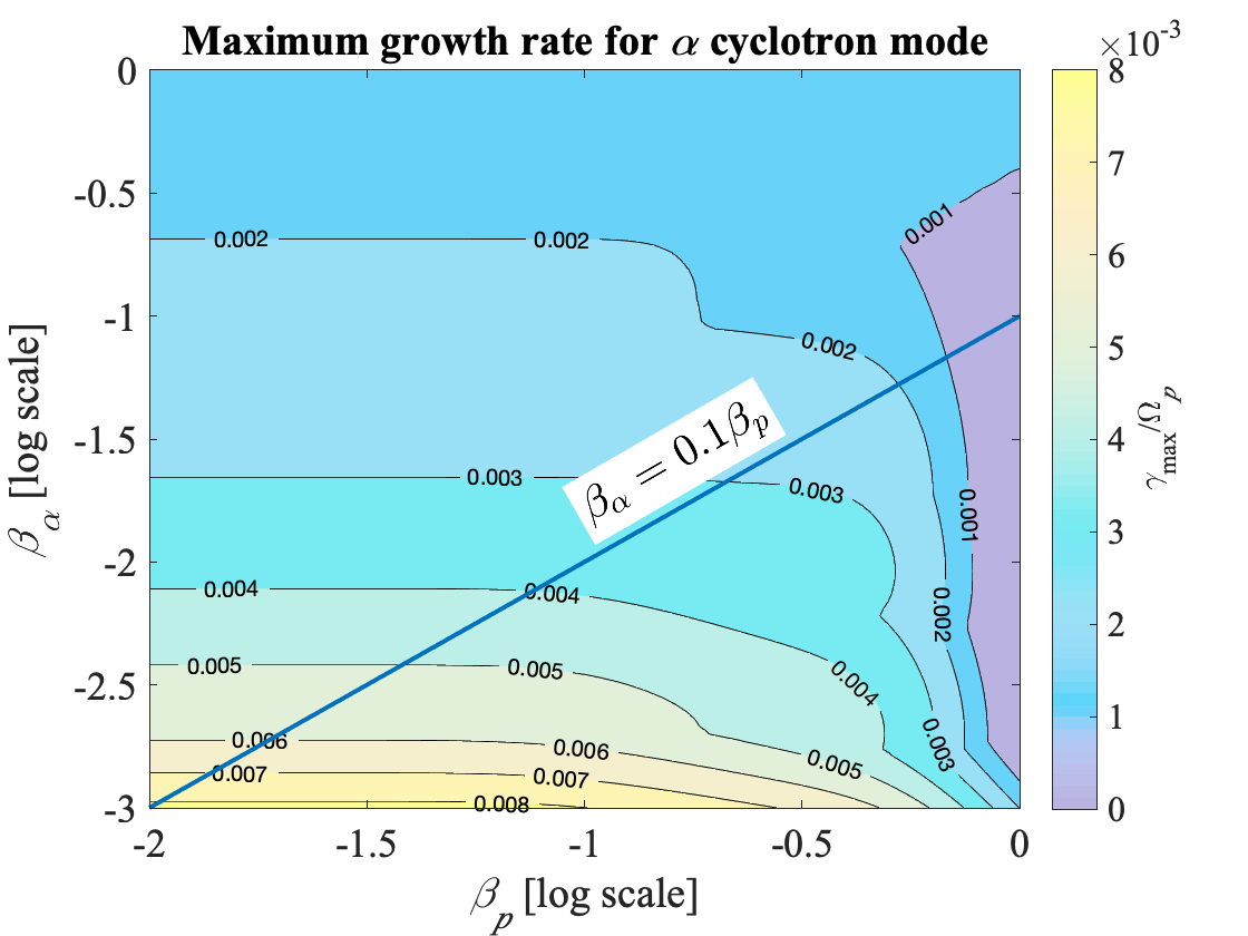
Fig. 3 : Maximum growth rate for alpha cyclotron mode branch versus $\beta_{p}$ and $\beta_{\alpha}$. Other parameters are fixed, $n_{\alpha}/n_{p}=0.05$ and $V_{\alpha}=v_{A}$.

To summarize, we find that the relative proton-alpha beam driven cyclotron instabilities of both the alpha cyclotron and proton cyclotron mode branches are generally confined to low beta regime, which in general conforms with measurements in the solar wind at low altitudes (Matteini et al., 2013; Maruca et al., 2012). Of the two modes, however, the dominant instability is that of the alpha cyclotron branch, so that in the nonlinear stage, we expect that the alpha cyclotron mode will dominate the dynamics. For higher beta values, the beam driven cyclotron instabilities are generally suppressed, which might explain why in the literature, the proton-alpha drift instabilities in the high beta regime have been typically studied in combination with temperature anisotropies of either the protons or alpha particles.

5 Conclusions

The alpha/proton beam instabilities can play an important role in constraining the beaming velocity of alpha particles, and may explain the deceleration of alpha particles in the solar wind with increasing distance from the Sun. Previous studies have explored in much detail the high beta plasma regime of these instabilities, clarifying the role of internal temperature anisotropies of protons or alpha particles, which may switch from Alfvénic instabilities for isotropic beams to an instability of fast-magnetosonic/whistler mode if alpha beam exhibit $T_{\perp}/T_{\parallel}<1$.

In this paper we have formulated a dissipative (kinetic) theory for the dispersion and stability of alpha/proton beams, and applied to low beta regime specific to solar wind conditions at low heliospheric distances closer to Sun. In this case early studies assume an intrinsic thermal anisotropy $T_{\perp}/T_{\parallel}$ for protons or alpha particles, which stimulates Alfvénic instabilities and prohibits any other instabilities to develop. Contrary to that, here we assumed alpha and proton beams with isotropic temperatures $T_{\perp}/T_{\parallel}=1$, in order to provide basic insights on the dispersion and stability of alpha/proton beams.

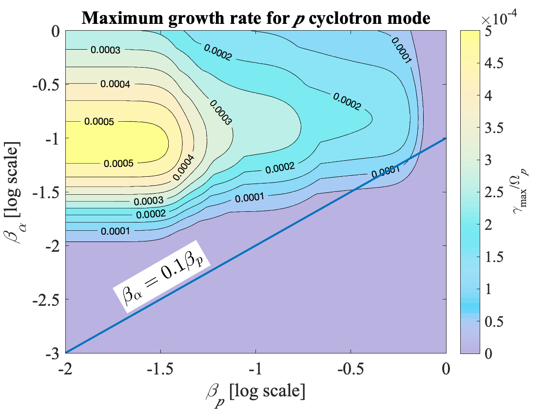
Fig. 4 : Maximum growth rate for proton cyclotron mode branch versus $\beta_{p}$ and $\beta_{\alpha}$. Other parameters are fixed, $n_{\alpha}/n_{p}=0.05$ and $V_{\alpha}=v_{A}$.

In Section 2, we have derived the general dispersion relations of electromagnetic waves propagating at arbitrary angle ($\theta$) with respect to the magnetic field. In Section 3, we formulated the weak growth rate theory for plasma particles that are assumed to be distributed according to standard (Maxwellian) statistics, with protons and alpha particles considered to be counter-drifting Maxwellians. In section 4 we have examined a sample growth rate calculation associated with the electromagnetic modes: fast-magnetosonic/whistler, proton-cyclotron and alpha-cyclotron waves, for a given set of alpha-to-proton density ratio, $n_{\alpha}/n_{p}$, alpha and proton beta’s, $\beta_{\alpha}$ and $\beta_{p}$, and alpha-proton relative drift speed, $V_{\alpha}$, which is fixed at $v_{A}$. The results unveiled a potential competition between instabilities of proton and alpha cyclotron modes, but the sample calculation also showed that the alpha cyclotron mode may reach growth rates one order of magnitude higher than that of the proton cyclotron mode. We have then proceeded with the calculation of maximum growth rates for each mode as we continuously varied $\beta_{\alpha}$ and $\beta_{p}$. It was shown that for the low beta solar wind conditions in the outer corona, the alpha cyclotron instability is the dominant mode, with growth rates increasing with decreasing $\beta_{\alpha}$. In contrast, the less unstable proton cyclotron mode has a local peak associated with the maximum growth rate around $\beta_{\alpha}=10^{-1}$, but the mode is suppressed for either decreasing or increasing $\beta_{\alpha}$ around this peaking value. Both modes, however, are stabilized by increasing proton beta, or equivalently, proton temperature.

The consequence of the excitation of these unstable modes on the solar wind proton and alpha particle dynamics cannot be understood purely on the basis of linear theory. In order to address such an issue, we will carry out quasilinear analysis in the near future. The impact of instability excitation on the radially expanding solar wind condition can also be studied in the future where, the the effects of radial expansion can be counter balanced by the wave-particle relaxation by instabilities. Such a task is a subject of our ongoing research.

Acknowledgements The authors acknowledge support from the Katholieke Universiteit Leuven (Grant No. SF/17/007, 2018), Ruhr-University Bochum, and Alexander von Humboldt Foundation. These results were obtained in the framework of the projects SCHL 201/35-1 (DFG–German Research Foundation), GOA/2015-014 (KU Leuven), G0A2316N (FWO-Vlaa- nderen), and C 90347 (ESA Prodex 9). M.A.R. acknowledges Punjab Higher Education Commission (PHEC) Pakistan for granted Postdoctoral Fellowship FY 2017-18. S.M.S. gratefully acknowledges support by a Postdoctoral Fellowship (Grant No. 12Z6218N) of the Research Foundation Flanders (FWO-Belgium). P.H.Y. acknowledges NASA Grant NNH18ZDA001N-HSR and NSF Grant 1842643 to the University of Maryland, and the BK21 plus program from the National Research Foundation (NRF), Korea, to Kyung Hee University.

Appendix A Polarization vector

For an ambient magnetic field vector directed along $z$ axis, $\hat{\bf b}={\bf B}_{0}/|B_{0}|=\hat{\bf z}$ and the wave vector lying in $xz$ plane, ${\bf k}=k_{\perp}\hat{\bf x}+k_{\parallel}\hat{\bf z}=\hat{\bf x}k\sin\theta+\hat{\bf z}k\cos\theta$, we define three orthogonal unit vectors, following (Melrose, 1986), $\hat{\bm{\kappa}}=\hat{\bf x}\sin\theta+\hat{\bf z}\cos\theta$, $\hat{\bf a}=\hat{\bf y}$, and $\hat{\bf t}=\hat{\bf x}\cos\theta-\hat{\bf z}\sin\theta$. Then the unit wave electric field vector is given by

$$\hat{\bf e}({\bf k})=\frac{\delta{\bf E}}{|\delta E|}=\frac{K\,\hat{\bm{\kappa}}+T\,\hat{\bf t}+i\,\hat{\bf a}}{(K^{2}+T^{2}+1)^{1/2}}.$$ (A1)

Making use of linear wave equation,

$$\left[\epsilon_{ij}-N^{2}\left(\delta_{ij}-k_{i}k_{j}/k^{2}\right)\right]\delta E_{j}=0,$$ (A2)

it is possible to obtain

$$\delta E_{x} =\frac{\epsilon_{xx}-N^{2}}{\epsilon_{xy}}\,\delta E_{y},$$

$$\delta E_{z} =-\frac{N^{2}\sin\theta\cos\theta}{\epsilon_{zz}-N^{2}\sin^{2}\theta}\frac{\epsilon_{xx}-N^{2}}{\epsilon_{xy}}\,\delta E_{y}.$$ (A3)

Upon direct comparison with Eq. (A1) one may identify

$$K =-\frac{i\sin\theta\,(\epsilon_{zz}-N^{2})\,\epsilon_{xy}}{\epsilon_{xx}\,\epsilon_{zz}-N^{2}\,A},$$

$$T =-\frac{i\cos\theta\,\epsilon_{zz}\,\epsilon_{xy}}{\epsilon_{xx}\,\epsilon_{zz}-N^{2}\,A},$$ (A4)

where $A=\epsilon_{xx}\sin^{2}\theta+\epsilon_{zz}\cos^{2}\theta$. Upon making use of Eq. (5), we further obtain

$$K =-M\sin\theta,\qquad T=-M\cos\theta,$$

$$M =\frac{x^{2}Q_{+}Q_{-}+\delta P_{+}P_{-}(x^{2}+\frac{1}{4})}{x^{2}D+q^{2}P_{+}P_{-}Q_{+}Q_{-}\mu^{2}},$$ (A5)

where various quantities, $P_{\pm}$, $Q_{\pm}$, and $D$, as well as normalized wave number and frequency, $q=ck/\omega_{pp}$ and $x=\omega/\Omega_{p}$, are defined in Eq. (8).

Appendix B Parameter $R$

In the growth rate expression (9) appears a quantity $\partial(\omega^{2}N^{2})/\partial\omega$, which in normalized form, is defined by

$$R=\frac{\Omega_{p}}{\omega_{pp}^{2}}\frac{\partial(\omega^{2}N^{2})}{\partial\omega}=\frac{\partial q^{2}}{\partial x}.$$ (B1)

Making use of Eqs. (6) and (8), the desired quantity $R$ can readily be computed as

$$R = \frac{x}{2P_{+}P_{-}Q_{+}Q_{-}q^{2}\mu^{2}+D(1+\mu^{2})x^{2}}$$ (B2)

$$\times\left[\left(\frac{2Q_{+}Q_{-}}{P_{+}P_{-}}+\frac{\delta}{2}\frac{P_{+}P_{-}}{Q_{+}Q_{-}}\right)q^{2}(1+\mu^{2})\right.$$

$$+2\delta^{2}P_{+}P_{-}Q_{+}Q_{-}+\frac{2x^{2}(x^{2}-2)Q_{+}Q_{-}}{P_{+}P_{-}}$$

$$\left.+\frac{\delta x^{2}}{4}\frac{8x^{4}(2x^{2}-5)+3(9x^{2}-2)}{P_{+}P_{-}Q_{+}Q_{-}}\right].$$

References

- Asbridge et al. (1976) Asbridge, J.R., Bame, S.J., Feldman, W.C., Montgomery, M.D.: J. Geophys. Res. 81(16), 2719 (1976). doi:10.1029/JA081i016p02719
- Gary (1993) Gary, S.P.: Theory of Space Plasma Microinstabilities. Cambridge University Press, Cambridge (1993). doi:10.1017/CBO9780511551512
- Gary et al. (2000a) Gary, S.P., Yin, L., Winske, D., Reisenfeld, D.B.: Journal of Geophysical Research: Space Physics 105(A9), 20989 (2000a)
- Gary et al. (2000b) Gary, S.P., Yin, L., Winske, D., Reisenfeld, D.B.: Geophys. Res. Lett. 27(9), 1355 (2000b)
- Gomberoff and Valdivia (2003) Gomberoff, L., Valdivia, J.A.: Journal of Geophysical Research: Space Physics 108(A1), 1050 (2003)
- Kasper et al. (2007) Kasper, J.C., Stevens, M.L., Lazarus, A.J., Steinberg, J.T., Ogilvie, K.W.: Astrophys. J. 660(1), 901 (2007)
- Kohl et al. (1998) Kohl, J.L., Noci, G., Antonucci, E., Tondello, G., Huber, M.C.E., Cranmer, S.R., Strachan, L., Panasyuk, A.V., Gardner, L.D., Romoli, M., Fineschi, S., Dobrzycka, D., Raymond, J.C., Nicolosi, P., Siegmund, O.H.W., Spadaro, D., Benna, C., Ciaravella, A., Giordano, S., Habbal, S.R., Karovska, M., Li, X., Martin, R., Michels, J.G., Modigliani, A., Naletto, G., Neal, R.H.O., Pernechele, C., Poletto, G., Smith, P.L., Suleiman, R.M.: Astrophys. J. 501(1), 127 (1998). doi:10.1086/311434
- Li and Habbal (1999) Li, X., Habbal, S.R.: Solar Physics 190(1-2), 485 (1999). doi:10.1023/A:1005288832535
- Maneva et al. (2014) Maneva, Y.G., Araneda, J.A., Marsch, E.: Astrophys. J. 783(2), 139 (2014). doi:10.1088/0004-637x/783/2/139
- Marsch and Livi (1987) Marsch, E., Livi, S.: J. Geophys. Res. 92(A7), 7263 (1987). doi:10.1029/JA092iA07p07263
- Marsch et al. (1982) Marsch, E., Mühlhäuser, K.-H., Rosenbauer, H., Schwenn, R., Neubauer, F.: J. Geophys. Res. 87(A1), 35 (1982)
- Marsch (1991) Marsch, E.: Kinetic Physics of the Solar Wind Plasma. Physics and Chemistry in Space, vol. 21, p. 45. Springer, Berlin, Heidelberg (1991)
- Marsch (2006) Marsch, E.: Living Rev. Solar Phys. 3(1), 1 (2006). doi:10.12942/lrsp-2006-1
- Maruca et al. (2012) Maruca, B.A., Kasper, J.C., Gary, S.P.: Astrophys. J. 748(2), 137 (2012)
- Matteini et al. (2013) Matteini, L., Hellinger, P., Goldstein, B.E., Landi, S., Velli, M., Neugebauer, M.: J. Geophys. Res. 118(6), 2771 (2013). doi:10.1002/jgra.50320
- Melrose (1986) Melrose, D.B.: Instabilities in Space and Laboratory Plasmas. Cambridge University Press, Cambridge (1986). doi:10.1017/CBO9780511564123
- Neugebauer (1981) Neugebauer, M.: Fundamentals of Cosmic Physics 7, 131 (1981)
- Reisenfeld et al. (2001) Reisenfeld, D.B., Gary, S.P., Gosling, J.T., Steinberg, J.T., McComas, D.J., Goldstein, B.E., Neugebauer, M.: J. Geophys. Res. 106(A4), 5693 (2001)
- Revathy (1978) Revathy, P.: J. Geophys. Res. 83(A12), 5750 (1978)
- Robbins et al. (1970) Robbins, D.E., Hundhausen, A.J., Bame, S.J.: J. Geophys. Res. 75(7), 1178 (1970)
- Stansby et al. (2019) Stansby, D., Perrone, D., Matteini, L., Horbury, T.S., Salem, C.S.: A&A 623, 2 (2019). doi:10.1051/0004-6361/201834900
- Verscharen et al. (2013) Verscharen, D., Bourouaine, S., Chandran, B.D.G., Maruca, B.A.: Astrophys. J. 773(1), 8 (2013)
- von Steiger et al. (1995) von Steiger, R., Geiss, J., Gloeckler, G., Galvin, A.B.: Space Sci. Rev. 72(1), 71 (1995). doi:10.1007/BF00768756