Transverse momentum dependent PDFs at N³LO

Abstract

We compute the quark and gluon transverse momentum dependent parton distribution functions at next-to-next-to-next-to-leading order (N³LO) in perturbative QCD. Our calculation is based on an expansion of the differential Drell-Yan and gluon fusion Higgs production cross sections about their collinear limit. This method allows us to employ cutting edge multiloop techniques for the computation of cross sections to extract these universal building blocks of the collinear limit of QCD. The corresponding perturbative matching kernels for all channels are expressed in terms of simple harmonic polylogarithms up to weight five. As a byproduct, we confirm a previous computation of the soft function for transverse momentum factorization at N³LO. Our results are the last missing ingredient to extend the $q_{T}$ subtraction methods to N³LO and to obtain resummed $q_{T}$ spectra at N³LL^′ accuracy both for gluon as well as for quark initiated processes.

1 Introduction

Transverse momentum dependent parton distribution functions (TMDPDFs) extend the concept of collinear PDFs, which describe the longitudinal momentum distribution of quarks and gluons inside protons, to also reflect their intrinsic transverse motion. They are important ingredients for describing high-energy scatterings at small transverse momentum, in particular the Drell-Yan process, an important benchmark observable of the Standard Model both at the Tevatron Affolder:1999jh ; Abbott:1999yd ; Abazov:2007ac ; Abazov:2010kn and the LHC Aad:2011gj ; Chatrchyan:2011wt ; Aad:2014xaa ; Khachatryan:2015oaa ; Aad:2015auj ; Khachatryan:2016nbe ; Sirunyan:2019bzr ; Aad:2019wmn . Similarly, they are required for predictions of the Higgs transverse momentum spectrum, a key observable that is of great interest for the LHC physics program Aad:2014lwa ; Aad:2014tca ; Aad:2016lvc ; Aaboud:2017oem ; Aaboud:2018xdt ; ATLAS:2020wny ; Khachatryan:2015rxa ; Khachatryan:2015yvw ; Khachatryan:2016vnn ; Sirunyan:2018kta ; Sirunyan:2018sgc . TMDPDFs also arise in measurements of semi-inclusive deep-inelastic scattering (SIDIS) Ashman:1991cj ; Derrick:1995xg ; Adloff:1996dy ; Aaron:2008ad ; Airapetian:2012ki ; Adolph:2013stb ; Aghasyan:2017ctw , where they are of particular interested because they provide a window into the proton structure Boer:2011fh ; Accardi:2012qut .

TMDPDFs measure both the longitudinal momentum fraction $z$ and the transverse momentum ${\vec{q}}_{T}$ carried by the struck parton. They are intrinsically nonperturbative objects that need to be extracted from measurements, but for perturbative $|{\vec{q}}_{T}|$ they can be perturbatively related to collinear PDFs. Schematically, this matching takes the form

$$B_{i}(z,{\vec{q}}_{T})=\sum_{j}\int_{z}^{1}\!\frac{\mathrm{d}z^{\prime}}{z^{\prime}}\,\mathcal{I}_{ij}(z^{\prime},{\vec{q}}_{T})f_{j}\Bigl{(}\frac{z}{z^{\prime}}\Bigr{)}\times\bigl{[}1+\mathcal{O}(q_{T}/\Lambda_{\mathrm{QCD}})\bigr{]}\,,$$ (1)

where $B_{i}$ is the so-called TMD beam function for a parton of flavor $i$, the sum runs over all parton flavors $j$, $\mathcal{I}_{ij}$ is the perturbative matching kernel, and $f_{j}$ is the collinear PDF. The precise knowledge of $\mathcal{I}_{ij}$ is important for measurements dominated by transverse momenta that are small compared to the hard scale $Q$ of the process but still perturbative, i.e. $\Lambda_{\mathrm{QCD}}\ll|{\vec{q}}_{T}|\ll Q$, such as Higgs and Drell-Yan production at the LHC. Precise perturbative predictions for the beam function are also essential to extract the intrinsically nonperturbative corrections, which in global fits is typically achieved through a nonperturbative model on top of eq. (1), see e.g. refs. Landry:1999an ; Landry:2002ix ; Konychev:2005iy ; DAlesio:2014mrz ; Bacchetta:2017gcc ; Scimemi:2017etj ; Scimemi:2019cmh .

Since TMDPDFs describe processes at small transverse momentum ${\vec{q}}_{T}$, they are intrinsically sensitive to the infrared structure of QCD. Hence, their perturbative structure is intimately related to the singular structure of QCD amplitudes. This property is employed in the $q_{T}$ subtraction scheme proposed in ref. Catani:2007vq to achieve the cancellation of infrared divergences in next-to-next-leading order (NNLO) calculations of color-singlet cross sections. Recently, extensions of this method to next-to-next-to-next-to-leading order (N³LO) were discussed in refs. Cieri:2018oms ; Billis:2019vxg , which however did not include the required three-loop ingredient.

TMDPDFs are composed of the TMD beam function $B_{i}(z,{\vec{q}}_{T})$ and the TMD soft function $S({\vec{q}}_{T})$. The soft function has been known at three loops since quite some time Echevarria:2015byo ; Li:2016ctv ; Luebbert:2016itl , and the quark beam function has been calculated at this accuracy recently Catani:2012qa ; Gehrmann:2012ze ; Gehrmann:2014yya ; Echevarria:2016scs ; Luo:2019hmp ; Luo:2019szz , while the gluon beam function so far is only known at two loops Catani:2011kr ; Gehrmann:2014yya ; Echevarria:2016scs ; Luo:2019bmw . In this paper, we fill this gap by calculating the full matching coefficient for the gluon beam function at N³LO. We also calculate the full quark beam function at N³LO, where we find disagreement with the recent calculation of the corresponding result in ref. Luo:2019szz in the $d_{abc}d^{abc}$ color structure. These results make it possible to fully apply the ${\vec{q}}_{T}$ subtraction at N³LO accuracy, paving the way for fully-differential cross sections of color-singlet processes at this order. Our results are also the last missing ingredient for TMD resummation at N³LL^′ accuracy. They also arise in ${\vec{q}}_{T}$-dependent event shapes at hadron colliders such as the Transverse Energy-Energy Correlator (TEEC) Gao:2019ojf , and for the azimuthal angle in vector boson $+j$ production in the back-to-back limit Chien:2019gyf ; Chien:2020hzh .

We perform the calculation of the TMDPDF at N³LO by using the framework of the collinear expansion of cross sections presented in Ebert:2020lxs . This framework allows us to efficiently compute universal building blocks of perturbative QFT in kinematic limits leveraging on modern technology developed for the computation of multiloop scattering cross sections. In particular, we expand the diagrams for the Drell-Yan and gluon fusion Higgs boson production cross section at N³LO in the collinear limit. We make use of the framework of reverse unitarity Anastasiou2003 ; Anastasiou:2002qz ; Anastasiou:2003yy ; Anastasiou2005 ; Anastasiou2004a to enforce measurement and on-shellness constraints on the final states as well as integration-by-part (IBP) identities Chetyrkin:1981qh ; Tkachov:1981wb and the method of differential equations Kotikov:1990kg ; Kotikov:1991hm ; Kotikov:1991pm ; Henn:2013pwa ; Gehrmann:1999as to obtain the cross sections differential in the rapidity and transverse momentum of the colorless final states in the collinear limit. Following ref. Ebert:2020lxs , we exploit this limit of the differential cross sections to extract the bare matching kernels of the quark and gluon ${\vec{q}}_{T}$ beam functions.

This paper is structured as follows. In section 2, we briefly review TMD factorization. In section 3, we discuss how the beam function can be calculated from the collinear limit of a color-singlet cross section using the method collinear expansions. In section 4, we present our results, before concluding in section 5. Our results are also available in electronic form in the ancillary files of this submission.

2 Review of $q_{T}$ factorization

We study the production of a color-singlet state $h$ and an additional hadronic state $X$ in a proton-proton scattering process,

$$P(P_{1})+P(P_{2})\quad\to\quad h(-p_{h})+X(-k)\,,$$ (2)

where we align the incoming protons along the directions

$$n^{\mu}=(1,0,0,1)\,,\qquad{\bar{n}}^{\mu}=(1,0,0,-1)$$ (3)

and denote their momenta as $P_{1}$ and $P_{2}$, with the center of mass energy being $S=(P_{1}+P_{2})^{2}$. We are interested in measuring the cross section differential in $p_{h}^{\mu}$, expressed through the invariant mass $Q^{2}=p_{h}^{2}$, rapidity $Y$, and transverse momentum ${\vec{q}}_{T}$.

The factorization of the cross section in the limit $q_{T}\ll Q$ was first established by Collins, Soper, and Sterman (CSS) Collins:1981uk ; Collins:1981va ; Collins:1984kg , and was further elaborated on in refs. Catani:2000vq ; deFlorian:2001zd ; Catani:2010pd ; Collins:1350496 . The factorization was also shown using Soft-Collinear Effective Theory (SCET) Bauer:2000ew ; Bauer:2000yr ; Bauer:2001ct ; Bauer:2001yt by several groups Becher:2010tm ; Becher:2011xn ; Becher:2012yn ; GarciaEchevarria:2011rb ; Echevarria:2012js ; Echevarria:2014rua ; Chiu:2012ir ; Li:2016axz . The factorized cross section is typically expressed in Fourier space in two equivalent forms,

$$\frac{\mathrm{d}\sigma}{\mathrm{d}Q^{2}\mathrm{d}Y\mathrm{d}^{2}{\vec{q}}_{T}} =\sigma_{0}\sum_{a,b}H_{ab}(Q^{2},\mu)\int\!\frac{\mathrm{d}^{2}{\vec{b}}_{T}}{(2\pi)^{2}}e^{\mathrm{i}\,{\vec{q}}_{T}\cdot{\vec{b}}_{T}}\,\tilde{B}_{a}\Bigl{(}x_{1}^{B},b_{T},\mu,\frac{\nu}{\omega_{a}}\Bigr{)}\,\tilde{B}_{b}\Bigl{(}x_{2}^{B},b_{T},\mu,\frac{\nu}{\omega_{b}}\Bigr{)}\,\tilde{S}(b_{T},\mu,\nu)$$

$$=\sigma_{0}\sum_{a,b}H_{ab}(Q^{2},\mu)\int\!\frac{\mathrm{d}^{2}{\vec{b}}_{T}}{(2\pi)^{2}}e^{\mathrm{i}\,{\vec{q}}_{T}\cdot{\vec{b}}_{T}}\,\tilde{f}_{a}(x_{1}^{B},b_{T},\mu,\zeta_{a})\,\tilde{f}_{b}(x_{2}^{B},b_{T},\mu,\zeta_{b})\,.$$ (4)

For processes inclusive in $h$, eq. (2) holds up to corrections in $\mathcal{O}(q_{T}^{2}/Q^{2})$. Power corrections of $\mathcal{O}(q_{T}^{2}/Q^{2})$ have been firstly calculated at fixed order in perturbation theory in ref. Ebert:2018gsn , while the study of their all order structure has been initiated using SCET operator formalism Kolodrubetz:2016uim ; Feige:2017zci ; Moult:2017rpl ; Chang:2017atu ; Chang:NLP and their nonperturbative structure has been explored in refs. Balitsky:2017gis ; Balitsky:2017flc . Eq. (2) receives enhanced $\mathcal{O}(q_{T}/Q)$ corrections when applying fiducial cuts to $h$ Ebert:2019zkb that can be uniquely included in the factorization for Higgs and Drell-Yan production Ebert:fiducial , and also receives linear corrections when radiation from massive final states is considered Buonocore:2019puv .

In eq. (2), we sum over all parton flavors $a$ and $b$ mediating the underlying partonic process $ab\to h$. The corresponding partonic Born cross section is denoted by $\sigma_{0}$, and the hard function $H_{ab}=1+\mathcal{O}(\alpha_{s})$ encodes virtual corrections to the Born process. For Drell-Yan and gluon fusion Higgs production in the $m_{t}\to\infty$ limit, the N³LO hard function can be found in ref. Gehrmann:2010ue , and for $b\bar{b}\to H$ in refs. Gehrmann:2014vha ; Ebert:2017uel . The $\tilde{B}_{i}(x,b_{T},\mu,\nu/\omega)$ encode the probability to find a parton of flavor $i$ with longitudinal momentum fraction $x$ and impact parameter ${\vec{b}}_{T}$, which is Fourier-conjugate to ${\vec{q}}_{T}$. The soft function $\tilde{S}$ encodes the effect of soft radiation from either proton. In the second line of eq. (2), these functions are combined into the TMDPDF

$$\tilde{f}_{i}(x,b_{T},\mu,\zeta)=\tilde{B}_{i}\Bigl{(}x,b_{T},\mu,\frac{\nu}{\sqrt{\zeta}}\Bigr{)}\sqrt{S(b_{T},\mu,\nu)}\,,$$ (5)

which is indepdent of the rapidity scale $\nu$ discussed below. Computationally, it is natural to separately consider the calculation of the beam and soft functions appearing in eq. (2), which can easily be combined into the TMDPDF if desired.

A characteristic feature of $q_{T}$ factorization is the appearance of so-called rapidity divergences Collins:1981uk ; Collins:2008ht ; Becher:2010tm ; GarciaEchevarria:2011rb ; Chiu:2011qc ; Chiu:2012ir ; Rothstein:2016bsq , which require an explicit rapidity regulator. Similar to the emergence of the renormalization scale $\mu$ from ultraviolet (UV) regularization, this induces a rapidity scale, which we generically as $\nu$. The rapidity divergences track the energy of the struck partons, encoded in the parameters

$$\omega_{a}=x_{a}\,{\bar{n}}\cdot P_{a}=Qe^{+Y}\,,\quad\omega_{b}=x_{b}\,n\cdot P_{b}=Qe^{-Y}\,,\qquad\zeta_{a,b}\propto\omega_{a,b}^{2}\quad\mathrm{s.t.}\quad\mathrm{\zeta}_{a}\zeta_{b}=Q^{4}\,.$$ (6)

There is a variety of rapidity regulators, giving rise to several formulations of the individual ingredients in eq. (2). However, all approaches yield the same fixed-order results for the physical cross section in eq. (2). Thus, we are free to choose the regulator most convenient for our calculation, and we will employ the exponential regulator of ref. Li:2016axz . Explicit definitions of the beam and soft functions in terms of gauge-invariant matrix elements formulated in SCET can be found in ref. Li:2016axz (see also refs. Luo:2019hmp ; Luo:2019bmw ), but are not required in our approach.

In this work, we focus on TMD factorization in the perturbative regime $b_{T}^{-1}\sim q_{T}\gg\Lambda_{\mathrm{QCD}}$, in which the TMD beam function and TMDPDF can be matched onto PDFs as Collins:1984kg

$$\tilde{B}_{i}\Bigl{(}z,b_{T},\mu,\frac{\nu}{\omega}\Bigr{)} =\sum_{j}\int_{z}^{1}\!\frac{\mathrm{d}z^{\prime}}{z^{\prime}}\,\tilde{\mathcal{I}}_{ij}\Bigl{(}z^{\prime},b_{T},\mu,\frac{\nu}{\omega}\Bigr{)}f_{j}\Bigl{(}\frac{z}{z^{\prime}},\mu\Bigr{)}\times\bigl{[}1+\mathcal{O}(b_{T}\Lambda_{\mathrm{QCD}})\bigr{]}\,,$$

$$\tilde{f}_{i}(z,b_{T},\mu,\zeta) =\sum_{j}\int_{z}^{1}\!\frac{\mathrm{d}z^{\prime}}{z^{\prime}}\,\tilde{\mathcal{I}}^{\rm TMD}_{ij}(z^{\prime},b_{T},\mu,\zeta)f_{j}\Bigl{(}\frac{z}{z^{\prime}},\mu\Bigr{)}\times\bigl{[}1+\mathcal{O}(b_{T}\Lambda_{\mathrm{QCD}})\bigr{]}\,.$$ (7)

The matching kernels $\tilde{\mathcal{I}}_{ij}$ and $\tilde{\mathcal{I}}^{\rm TMD}_{ij}$ are the objects of interest of this paper.

3 Beam functions from the collinear limit of cross sections

We consider the contribution to eq. (2) from the partonic process

$$i(p_{1})+j(p_{2})\quad\to\quad h(-p_{h})+X_{n}(-p_{3},\dots,-p_{n+2})\,.$$ (8)

The incoming partons carry momentum $p_{1}$ and $p_{2}$ and flavor $i$ and $j$, respectively, while we denote with $X_{n}$ the hadronic final state with total momentum $k$, consisting of $n$ partons with momenta $\{-p_{3},\dots,-p_{n+2}\}$, such that $k=\sum_{i\geq 3}p_{i}$. Note that at tree level we have $n=0$.

The final-state momenta are parameterized in terms of

$$Q^{2}=p_{h}^{2}\,,\quad Y=\frac{1}{2}\ln\frac{{\bar{n}}\cdot p_{h}}{n\cdot p_{h}}\,,\quad{w_{1}}=-\frac{\bar{n}\cdot k}{\bar{n}\cdot p_{1}}\,,\quad{w_{2}}=-\frac{n\cdot k}{n\cdot p_{2}}\,,\quad x=\frac{k^{2}}{(\bar{n}\cdot k)(n\cdot k)}\,,$$ (9)

where $Y$ is the rapidity of the color-singlet state $h$ and $Q^{2}$ its invariant mass.

The partonic cross section differential in these variables is defined as

$$\frac{\mathrm{d}\eta_{ij}}{\mathrm{d}Q^{2}\mathrm{d}{w_{1}}\mathrm{d}{w_{2}}\mathrm{d}x} =\frac{1}{\sigma_{0}}\frac{\mathcal{N}_{ij}}{2S}\sum_{X_{n}}\int\frac{\mathrm{d}\Phi_{h+n}}{\mathrm{d}{w_{1}}\mathrm{d}{w_{2}}\mathrm{d}x}\,|\mathcal{M}_{ij\to h+X_{n}}|^{2}\,.$$ (10)

Here $\mathrm{d}\Phi_{h+n}$ represents the differential phase space measure for the $h+X_{n}$ state, $|\mathcal{M}_{ij\to h+X_{n}}|^{2}$ is the squared matrix element for the partonic process in eq. (8), summed over the colors and helicities of the particles, with $\mathcal{N}_{ij}$ containing the helicity and color average of the incoming particles, and we normalize the expression by $\sigma_{0}$, the partonic Born cross section. The interested reader can find explicit expressions for $\mathcal{N}_{ij}$ and $\mathrm{d}\Phi_{h+n}$ in ref. Ebert:2020lxs .

In ref. Ebert:2020lxs , we showed that the matching coefficient in eq. (2) is obtained by taking the limit of eq. (10) where all real and loop momenta are treated as being collinear to $n$-direction, which is referred as the strict $n$-collinear limit, and we refer to ref. Ebert:2020lxs for details on its calculation:

$$\mathcal{I}_{ij}^{\rm naive}(z,q_{T})=\int_{0}^{1}\mathrm{d}x\int_{0}^{\infty}\mathrm{d}{w_{1}}\mathrm{d}{w_{2}}\, \delta[z-(1-{w_{1}})]\,\delta\Big{[}q_{T}^{2}-\frac{{w_{1}}{w_{2}}}{1-{w_{1}}}(1-x)Q^{2}\Bigr{]}$$

$$\times\,\lim\limits_{\mathrm{strict}~{}n-\mathrm{coll.}}\frac{\mathrm{d}\eta_{ij}}{\mathrm{d}Q^{2}\mathrm{d}{w_{1}}\mathrm{d}{w_{2}}\mathrm{d}x}\,.$$ (11)

Solving the $\delta$ functions fixes ${w_{1}}$ and ${w_{2}}$ as

$${w_{1}}=1-z\,,\quad{w_{2}}=\frac{q_{T}^{2}}{Q^{2}}\frac{z}{(1-x)(1-z)}\,.$$ (12)

The superscript ^naive in eq. (3) indicates that further steps are required to obtain the desired matching kernel. First, we note that the integral in eq. (3) contains the aforementioned rapidity divergences, namely divergences as $x\to 1$ or $z\to 1$ that are not regulated by dimensional regularization. We regulate these using the exponential regulator of ref. Li:2016axz , which in fact is the only regulator in the literature compatible with our approach. Inserting the regulator factor $\exp(2\tau e^{-\gamma_{E}}k^{0})$ expressed in the above variables, we obtain the regulated kernel as Ebert:2020lxs

$$\mathcal{I}_{ij}(z,q_{T},\epsilon,\tau/\omega)=\lim_{\begin{subarray}{c}\tau\to 0\\ \epsilon\to 0\end{subarray}}\int_{0}^{1}\mathrm{d}x \,\frac{z}{Q^{2}(1-x)(1-z)}\exp\left[-\tau e^{-\gamma_{E}}\frac{q_{T}^{2}}{\omega}\frac{z}{(1-x)(1-z)}\right]$$

$$\times\lim\limits_{\mathrm{strict}~{}n-\mathrm{coll.}}\frac{\mathrm{d}\eta_{ij}}{\mathrm{d}Q^{2}\mathrm{d}{w_{1}}\mathrm{d}{w_{2}}\mathrm{d}x}\biggl{|}_{\eqref{eq:vars_LP}}\,.$$ (13)

Here, $\omega=Qe^{Y}$ is the so-called label momentum. The exponential factor in eq. (3) regulates divergences as $x,z\to 1$, with $\tau$ being the rapidity regulator. UV and IR divergences are regulated by working in $d=4-2\epsilon$ dimensions, with the limit $\epsilon\to 0$ being taken after the limit $\tau\to 0$, as indicated. It is convenient to expand the exponential factor in eq. (3) in terms of distributions before carrying out the integral Luo:2019hmp , and we provide more details on this in appendix A.1.

It is common to express TMD beam functions in Fourier space, where convolutions in ${\vec{q}}_{T}$ are replaced by simple products, which in particular greatly simplifies the resummation of large logarithms Ebert:2016gcn . Denoting the Fourier-transform matching kernel as $\tilde{\mathcal{I}}_{ij}$, we obtain the renormalized kernel as

$$\tilde{\mathcal{I}}_{ij}(z,b_{T},\mu,\nu/\omega)=\sum_{k}\int_{z}^{1}\!\frac{\mathrm{d}z^{\prime}}{z^{\prime}}\,\Gamma_{jk}\Bigl{(}\frac{z}{z^{\prime}},\epsilon\Bigr{)}\,\tilde{Z}_{B}^{i}(\epsilon,\mu,\nu/\omega)\,\hat{Z}_{\alpha_{s}}(\mu,\epsilon)\,\frac{\tilde{\mathcal{I}}_{ik}(z^{\prime},b_{T},\epsilon,\tau)}{\tilde{S}(b_{T},\epsilon,\tau)}.$$ (14)

Here, following ref. Li:2016ctv we identify $\nu\equiv 1/\tau$ as the rapidity renormalization scale Chiu:2012ir . The so-called zero-bin subtraction Manohar:2006nz to subtract overlap of the beam function with the soft function is implemented by dividing by the soft function $\tilde{S}$ Luo:2019hmp . In eq. (14), the counterterm $\hat{Z}_{\alpha_{s}}$ implements the renormalization of the bare coupling constant $\alpha_{s}^{b}$ in the $\overline{\mathrm{MS}}$ scheme as stated in eq. (40). Infrared divergences are canceled through the convolution with the PDF counterterm $\Gamma_{jk}$, which is given in eq. (41). The remaining poles in $\epsilon$ are of UV nature in SCET and are thus canceled by an additional UV counter term in the effective theory, which is the beam function counter term $\tilde{Z}_{B}$.

Since the bare soft function is not given in the literature, we have directly calculated it from the soft limit of eq. (10) similar to eq. (3).

$$S(q_{T},\epsilon,\tau)=\lim_{\begin{subarray}{c}\tau\to 0\\ \epsilon\to 0\end{subarray}} \int_{0}^{1}\mathrm{d}x\int_{0}^{\infty}\,\mathrm{d}w_{1}\mathrm{d}w_{2}\,\delta\bigl{[}q_{T}^{2}-{w_{1}}{w_{2}}(1-x)Q^{2}\bigr{]}$$

$$\times\exp\bigl{[}-2Q\tau e^{-\gamma_{E}}({w_{1}}+{w_{2}})\bigr{]}\lim\limits_{\text{strict soft}}\frac{\mathrm{d}\eta_{ij}}{\mathrm{d}Q^{2}\mathrm{d}{w_{1}}\mathrm{d}{w_{2}}\mathrm{d}x}\,.$$ (15)

In the strict soft limit, both ${w_{1}}$ and ${w_{2}}$ are treated as small quantities, such the measurement $\delta$ function and the exponential regulator in eq. (3) are simpler than in eq. (3). The Fourier transform of eq. (3) yields the bare soft function $\tilde{S}(b_{T},\epsilon,\tau)$ required in eq. (14). We have also verified that the renormalized soft function reproduces the N³LO result of ref. Li:2016ctv . Since the bare soft function in the exponential regulator is only given at NLO in the literature Li:2016axz , we provide the bare soft function in electronic format in the ancillary files.

The strict soft limit of the general differential partonic coefficient function is obtained by expanding the strict collinear limit in $w_{1}$ and maintaining only the first term of the generalised power series. At $n^{th}$ order in perturbation theory the strict soft limit of the partonic coefficient function takes the form

$$\lim\limits_{\text{strict soft}}\frac{\mathrm{d}\eta_{ij}^{(n)}}{\mathrm{d}Q^{2}\mathrm{d}{w_{1}}\mathrm{d}{w_{2}}\mathrm{d}x}=\omega_{1}^{-1-n\epsilon}\omega_{2}^{-1-n\epsilon}\eta^{(n)}_{\text{strict soft}}(x,\epsilon),$$ (16)

where $\eta^{(n)}_{\text{strict soft}}(x,\epsilon)$ is independent of $w_{1}$ and $w_{2}$. Note that eq. (16) is related to the bare fully-differential soft function which measures the total soft radiation in a process. This limit is also easily related to the bare threshold soft function Li:2014afw via

$$S_{\text{thr}}^{(n)}(z,\epsilon)=\int_{0}^{\infty}\mathrm{d}w_{1}\,\mathrm{d}w_{2}\int_{0}^{1}\mathrm{d}x\,\delta(1-z-w_{1}-w_{2})\eta^{(n)}_{\text{strict soft}}(x,\epsilon)\,,$$ (17)

where $z$ is the threshold parameter. We have used this relation as an additional check on our soft limit.

4 Results

Here, we present our results for the matching kernels of the TMD beam functions at N³LO. Our calculation leverages on the collinear expansion of the cross sections for off-shell photon production (Drell-Yan) and Higgs production in gluon fusion in proton-proton collisions. The computation of the Higgs boson production cross section is performed in the heavy top quark effective theory where the gluons are directly coupled to the Higgs boson via an effective operator generated by integrating out the top quark field from the SM Lagrangian Inami1983 ; Shifman1978 ; Spiridonov:1988md ; Wilczek1977 ; Chetyrkin:1997un ; Schroder:2005hy ; Chetyrkin:2005ia ; Kramer:1996iq ; Kniehl:2006bg . The matrix elements for this computation can be categorized by the number of final state partons in addition to the color singlet final state. The relevant matrix elements for the calculation of the N³LO differential cross sections in the collinear limit involve one (RVV), two (RRV) and three (RRR) final state partons.

The results for the partonic cross sections involving matrix elements with exactly one parton in the final state are available in full kinematics from refs. Duhr:2020seh ; Dulat:2014mda ; Dulat:2017brz ; Dulat:2017prg which build on previous work done in refs. Anastasiou:2013mca ; Duhr:2014nda ; Duhr:2013msa . Therefore, in order to obtain the RVV contributions in the strict collinear limit, we can straightforwardly expand the results in full kinematics and extract the required components.

To compute the collinear limit of the partonic cross sections with more than one final state parton, the necessary Feynman diagrams are obtained using QGRAF Nogueira_1993 . We carry out the spinor and color algebra using an in-house code, and perform the strict collinear expansion of these matrix elements following the procedure outlined in ref. Ebert:2020lxs . In order to integrate over loop and phase space momenta with measurement and on-shell constraints, we make use of the framework of reverse unitarity Anastasiou2003 ; Anastasiou:2002qz ; Anastasiou:2003yy ; Anastasiou2005 ; Anastasiou2004a .

We re-express our expanded cross section in terms of master integrals (MI) via integration-by-parts (IBP) identities Chetyrkin:1981qh ; Tkachov:1981wb . We obtain a basis of 492 MI, expressed in terms of the variables in eq. (9) as well as the dimensional regularization parameter $\epsilon$, of which 172 MI are required to describe the RRV contributions, while 320 are needed for the RRR ones. In order to compute the collinear master integrals we employ the method of differential equations Kotikov:1990kg ; Kotikov:1991hm ; Kotikov:1991pm ; Henn:2013pwa ; Gehrmann:1999as . We fix the boundary conditions for the differential equations by further expanding the collinear master integrals in the soft limit and integrating over the phase space, such that the result of this procedure can then be easily matched to the soft integrals calculated in refs. Anastasiou:2013srw ; Anastasiou:2014lda ; Anastasiou:2014vaa ; Anastasiou:2015yha ; Duhr:2019kwi .

Completing these steps we obtain the bare differential partonic cross section expanded in the strict collinear limit of eq. (10). We note that the ingredients computed so far are the same as those neeeded for the calculation of the N³LO $N-$jettiness beam functions of ref. Ebert:2020unb . Next, we obtain the bare matching kernel via eq. (3) and subsequently perform the Fourier transform over ${\vec{q}}_{T}$ using eq. (28). Both the calculation of the differential partonic cross section as well as the extration of the ${\vec{q}}_{T}$-dependent matching kernels will be elaborated in ref. Ebert:ThingsToCome . Finally, the renormalized matching kernel is obtained using eq. (14), where the beam function counter term $\tilde{Z}_{B}^{i}$ was predicted from the renormalization group equations (RGEs) of the beam function as shown in appendix A.4. The TMDPDF can then be straightforwardly obtained by combining the beam function with the soft function as in eq. (5).

We expand the matching kernels $\tilde{\mathcal{I}}_{ij}$ of the beam function and the matching kernels $\tilde{\mathcal{I}}^{\rm TMD}_{ij}$ of the TMDPDF obtained in this way in powers of $\alpha_{s}/\pi$,

$$\tilde{\mathcal{I}}_{ij}(z,b_{T},\mu,\nu/\omega) =\sum_{\ell=0}^{\infty}\Bigl{(}\frac{\alpha_{s}}{\pi}\Bigr{)}^{\ell}\tilde{\mathcal{I}}_{ij}^{(\ell)}(z,b_{T},\mu,\nu/\omega)\,,$$

$$\tilde{\mathcal{I}}^{\rm TMD}_{ij}(z,b_{T},\mu,\zeta) =\sum_{\ell=0}^{\infty}\Bigl{(}\frac{\alpha_{s}}{\pi}\Bigr{)}^{\ell}\tilde{\mathcal{I}}^{\mathrm{TMD}\,(\ell)}_{ij}(z,b_{T},\mu,\zeta)\,,$$ (18)

where the coefficients $\tilde{\mathcal{I}}_{ij}^{(\ell)}$ and $\tilde{\mathcal{I}}^{\mathrm{TMD}~{}(\ell)}_{ij}$ can be written as a polynomial in logarithms of the appearing scales with $z$-dependent coefficient functions,

$$\tilde{\mathcal{I}}_{ij}^{(\ell)}(z,b_{T},\mu,\nu/\omega) =\sum_{m,n=0}^{\ell}\tilde{\mathcal{I}}_{ij}^{(\ell,m,n)}(z)L_{b}^{n}L_{\omega}^{m}\,,$$ (19)

$$\tilde{\mathcal{I}}^{\mathrm{TMD}\,(\ell)}_{ij}(z,b_{T},\mu,\zeta) =\sum_{n=0}^{2\ell}\sum_{m=0}^{\ell}\tilde{\mathcal{I}}^{\mathrm{TMD}~{}(\ell,m,n)}_{ij}(z)L_{b}^{n}L_{\zeta}^{m}\,.$$

The logarithms in eq. (19) are defined as

$$L_{b}=\ln\frac{b_{T}^{2}\mu^{2}}{4e^{-2\gamma_{E}}}\,,\qquad L_{\omega}=\ln\frac{\nu}{\omega}\,,\qquad L_{\zeta}=\ln\frac{\mu^{2}}{\zeta}\,,$$ (20)

where $\gamma_{E}$ is the Euler-Mascheroni constant, and we remind the reader that $\zeta=\omega^{2}$ is the energy of the struck parton. The logarithmic terms with $m>0$ or $n>0$ in eq. (19) fully describe the scale dependence of both the TMDPDF as well as of the beam function. Therefore, their structure is completely determined by the beam function RGEs (see appendix A.3) in terms of its anomalous dimensions and lower-order ingredients. The nonlogarithmic beam function boundary term at N³LO

$$\tilde{I}_{ij}^{(3)}(z)\equiv\tilde{\mathcal{I}}_{ij}^{(3,0,0)}(z)\,,$$ (21)

is the genuinely new result calculated by us in this work. Remarkably, it can be expressed entirely in terms of standard plus distributions and harmonic polylogarithms Remiddi:1999ew of argument $z$ and transcendental weight less or equal to five. To allow for an easy numeric implementation, we also provide a generalized power series expansion of our results around $z=0$ and $z=1$ with up to 50 terms in each expansion. Both expansions formally converge in the unit interval, but, clearly, the convergence of the series improves as the expansion parameter gets smaller. In the ancillary files of the arXiv submission of this article we provide both power series as well as the analytic solution for all matching kernels.

We performed several checks on our results. Firstly, we verified that the UV and IR subtraction as given in eq. (14) correctly removes all poles in $\epsilon$. Our NLO and NNLO results for the renormalized beam function are validated against ref. Luebbert:2016itl , and the bare results through $\mathcal{O}(\epsilon^{4})$ at NLO and through $\mathcal{O}(\epsilon^{2})$ are verified against refs. Luo:2019hmp ; Luo:2019bmw . Given that the logarithmic terms in eq. (19) are dictaded by the beam function RGE, we verify that all logarithmic terms of our result are correct by comparing them against those predicted in ref. Billis:2019vxg by solving the beam function RGE. We also verified the eikonal limit

$$\lim_{z\to 1}\tilde{I}_{ij}^{(3)}(z) =\frac{\gamma_{2}^{r}}{64}\,\delta_{ij}\,\mathcal{L}_{0}(1-z)\,,$$ (22)

which was derived in ref. Billis:2019vxg from consistency with joint $q_{T}$ and soft threshold resummation relations Li:2016axz ; Lustermans:2016nvk , and also conjectured in ref. Echevarria:2016scs . In eq. (22), $\gamma_{2}^{r}$ is the three-loop coefficient of the so-called rapidity anomalous dimension Chiu:2012ir , as given in Eq. (16) of ref. Li:2016ctv (see also ref. Vladimirov:2016dll ), where the appropriate color structure is implicit. The rapidity anomalous dimensions is also closely related to the Collins-Soper kernel of refs. Collins:1981uk ; Collins:1981va . For the quark beam function, we also compared with the results recently obtained in ref. Luo:2019szz . We find discrepancies for terms proportional to the color structure $d^{abc}d_{abc}$ entering in all quark-to-quark kernels. After private communication, the authors of ref. Luo:2019szz identified and resolved a minor mistake in their calculation, after which they find agreement with our result. Furthermore, another check of our results comes from the fact that the first four terms in the soft expansion of the Higgs cross section correctly match the collinear limit of the threshold expansion of the partonic cross section obtained in  ref. Dulat:2017prg ; Dulat:2018bfe . We also note that inclusive cross section for Drell-Yan as well as for Higgs production at N³LO was calculated in refs. Anastasiou:2015ema ; Duhr:2020seh ; Mistlberger:2018etf ; Anastasiou:2014lda ; Anastasiou:2014vaa . Using the collinear partonic coefficient functions of our calculation after integration over phase space, we also correctly reproduce the leading threshold expansion contribution of all partonic initial states that contribute to the collinear limit of the partonic cross sections.

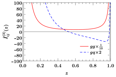
Figure 1: The N³LO beam function boundary term $\tilde{I}^{(3)}_{ij}(z)$ as a function of $z$ in all channels contributing to the quark beam function (left) and the gluon beam function (right). The different channels are rescaled as indicated in the figures.

Let us numerically illustrate our results. In figure 1 we plot the beam function boundary terms $\tilde{I}_{ij}(z)$ for the quark (left) and gluon (right) beam functions as a function of $z$. Note that in this plot we set $\delta(1-z)\to 0$ and replaced the distribution $\mathcal{L}_{0}(1-z)\to(1-z)^{-1}$. For illustration purposes we rescaled the different channel as indicated, given that they give rise to very different shapes and magnitudes.

Next, we study the impact of our calculation on the beam function and TMDPDF themselves. We use the MMHT2014nnlo68cl PDF of ref. Harland-Lang:2014zoa , using $\alpha_{s}(m_{Z})=0.118$ and the evaluation of eq. (2) is obtained through an implementation of our results in SCETlib scetlib .

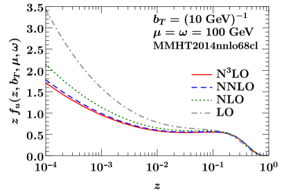
Figure 2: The $u$-quark TMDPDF (left) and the gluon TMDPDF (right) as a function of $z$ for fixed $b_{T}=(10~{}\,\mathrm{GeV})^{-1}$ and $\mu=\omega=100~{}\,\mathrm{GeV}$. We show the result at LO (which corresponds to the PDF), NLO, NNLO and N³LO.

In figure 2, we show the $u$-quark TMDPDF (left) and the gluon TMDPDF (right) at different orders in the coupling constant as a function of $z$. We fix the impact parameter $b_{T}=10~{}\,\mathrm{GeV}^{-1}$, parton energy $\omega=100~{}\,\mathrm{GeV}$ and renormalization scale $\mu=100~{}\,\mathrm{GeV}$. Since the LO result for the beam function corresponds to the PDF itself, figure 2 can be used to appreciate the difference in shape of the beam function compared to the PDF. With the inclusion of the N³LO result obtain in this work, both the quark and the gluon TMDPDFs nicely show convergence over a large range of values for $z$.

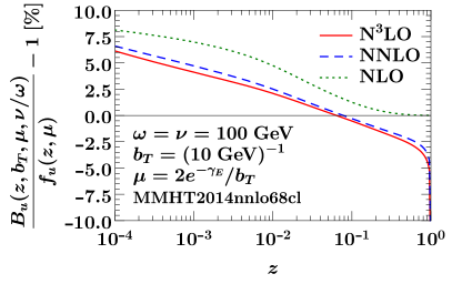
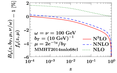
Figure 3: The relative difference of $u$-quark beam function (left) and the gluon beam function (right) to the corresponding PDF, as a function. We fix $b_{T}=(10~{}\,\mathrm{GeV})^{-1}$ and $\omega=100~{}\,\mathrm{GeV}$ and choose the canonical scales $\mu b_{T}=2e^{-\gamma_{E}}$ and $\nu=\omega$. Note that with this choice of scales, the displayed beam function is the boundary term of a resummed prediction.

In order to understand the impact of the new three-loop boundary term $\tilde{I}_{ij}^{(3)}$ in a resummed predictions, we present the beam function evaluated at the canonical scales $\mu b_{T}=2e^{-\gamma_{E}}$ and $\nu=\omega$, where all logarithms in eq. (19) vanish and only the boundary term $\tilde{I}_{ij}^{(3)}$ contributes. In figure 3, we compare the $u$-quark beam function (left) and gluon beam function (right) order by order in $\alpha_{s}$, up to N³LO, to the corresponding PDFs, choosing canonical scales for $b_{T}=(10~{}\,\mathrm{GeV})^{-1}$ and $\omega=100~{}\,\mathrm{GeV}$. We see that the beam function has a very different shape compared to the PDF, and that the beam function converges very well at N³LO.

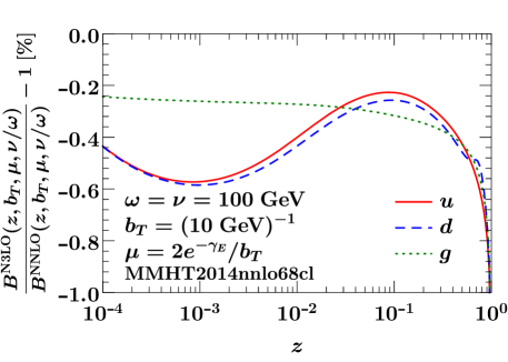
Figure 4: The $K$-factor of the N³LO beam function, i.e. the ratio of the N³LO beam function to NNLO beam function. We fix $b_{T}=(10~{}\,\mathrm{GeV})^{-1}$ and $\omega=100~{}\,\mathrm{GeV}$ and choose the canonical scales $\mu b_{T}=2e^{-\gamma_{E}}$ and $\nu=\omega$, such that the shown beam function corresponds to the boundary term in a resummed prediction. The different colors show the results for an $u$-quark, $d$-quark and gluon, respectively.

Finally, the $K$-factor of the N³LO beam function, which is defined as the ratio of the beam function at N³LO w.r.t. its value at NNLO, is shown in figure 4. As before, we choose the canonical scales for $b_{T}=(10~{}\,\mathrm{GeV})^{-1}$ and $\omega=100~{}\,\mathrm{GeV}$. We find a rather small correction of $\sim 0.2-0.5\%$, but with a notable dependence on $z$ for all channels.

For completeness, we also present the high-energy limit $z\to 0$ of the kernels $\tilde{I}_{gg}^{(3)}(z)$ and $\tilde{I}_{gq}^{(3)}(z)$ contributing to the gluon beam function in appendix B. The corresponding limit for the quark kernels were already presented in ref. Luo:2019szz , for which we find perfect agreement. These results are useful to study the small-$x$ behavior of TMDPDFs, see e.g. refs. Balitsky:2015qba ; Marzani:2015oyb ; Balitsky:2016dgz ; Xiao:2017yya .

5 Conclusions

We have calculated the perturbative matching kernel relating transverse-momentum dependent beam functions with lightcone PDFs at N³LO in QCD. This provides the first results of these kernels for the gluon TMD beam function, and corrects the result in the $d_{abc}d^{abc}$ color structure in the recent calculation of the quark TMD beam function in ref. Luo:2019szz . After private communication, the authors of ref. Luo:2019szz identified and resolved a minor mistake in their calculation, after which perfect agreement is found. This emphasizes that having two independent computations that are in accordance with each other is the most stringent cross check. Our results are obtained via a framework recently developed by us that allows for the efficient expansion of differential hadronic collinear cross sections Ebert:2020lxs , showing its applicability for the extraction of universal ingredients arising in the collinear limit of QCD to an unprecedented level of precision in perturbation theory. As a byproduct, we also confirmed a previous computation of the soft function for transverse momentum factorization Li:2016axz .

The results of our calculation are provided in the ancillary files of this paper submission. We include, for all quark and gluon channels, the renormalized TMD beam functions, along with their expansions around $z=0$ and $z=1$ up to 50 orders in each expansion, as well as the renormalized TMDPDFs and the bare and renormalized soft function.

The phenomenological applications of our results are numerous. Firstly, we provide the last missing ingredient for the fully-differential calculation of color-singlet processes at N³LO using the $q_{T}$ subtraction method Catani:2007vq ; Cieri:2018oms ; Billis:2019vxg , which can be used to obtain the first exact fully-differential cross sections at this order. They also enable the resummation of transverse momentum distributions at hadron colliders at N³LL^′ accuracy, both for gluon and quark induced hard scatterings such as Higgs-boson production and the Drell-Yan process, two key observables at the LHC.

A natural future direction of this research is the calculation of the closely related TMD fragmentation functions at N³LO, which are required to describe the small-$q_{T}$ limit semi-inclusive deep inelastic scattering and are currently only known at NNLO Echevarria:2016scs ; Luo:2019bmw ; Luo:2019hmp .

With the same techniques presented in this work, it would also be interesting to consider the calculation of other ${\vec{q}}_{T}$-dependent time-like collinear functions, such as the Energy-Energy Correlator (EEC) jet functions. The quark and gluon EEC jet functions enter the factorization of the EEC in the back-to-back limit for $e^{+}e^{-}$ annihilation and gluon initiated Higgs decay, respectively Moult:2018jzp , as well as that for the TEEC Gao:2019ojf . Their knowledge at N³LO is the only missing ingredient to achieve resummation of the EEC in the back-to-back limit at N³LL^′ accuracy. Note that at fixed order the full angle EEC has been calculated analytically through $\mathcal{O}(\alpha_{s}^{2})$ Dixon:2018qgp ; Luo:2019nig .

It will also be interesting to study the collinear expansions beyond leading power to shed light on the structure of TMD factorization at subleading power, in particular on the structure of rapidity divergences at subleading power Moult:2017xpp ; Ebert:2018gsn ; Moult:2019vou .

Appendix A Ingredients for the calculation of the beam function

In this appendix, we provide more details on the regularization and renormalization of the beam function kernels. Details of the calculation of all required integrals will be presented in ref. Ebert:ThingsToCome .

A.1 Rapidity regularization

In practice, it is useful to expand the regulator in eq. (3) in terms of plus distributions, which allows one to take the limit $\tau\to 0$ before evaluating the integral in eq. (3), see also Luo:2019hmp for a discussion at two loops. In general we want to expand a power divergence using the relation

$$\lim\limits_{\tau\to 0}\int_{0}^{1}\mathrm{d}x\,e^{-\tau/x}\frac{f(x)}{x^{1-a}}=\int_{0}^{1}\mathrm{d}x\left(f(0)\,\delta(x)\lim\limits_{\tau\to 0}G(\tau)+f(x)\left[\frac{1}{x^{1-a}}\right]_{+}\right).$$ (23)

Here, $f(x)$ is a suitable test function that is holomorphic at $x=0$ and $a$ represents a generalized power, typically proportional to the dimensional regulator $\epsilon$. We find that

$$G(\tau)=\int_{0}^{1}\mathrm{d}x\,\frac{e^{-\tau/x}}{x^{1-a}}=\frac{1}{a}\bigl{[}1-\tau^{a}\Gamma(1-a)\bigr{]}+\mathcal{O}(\tau).\\$$ (24)

We furthermore require the two-dimensional generalization of the above integral,

$$\int_{0}^{1}\!\mathrm{d}x\,\mathrm{d}y\,e^{-\tau/(xy)}x^{-1+a}y^{-1+b} = \frac{1}{ab}-\frac{\tau^{a}\Gamma(-a)}{a-b}+\frac{\tau^{b}\Gamma(-b)}{a-b}+\mathcal{O}(\tau)$$ (25)

The regularization of an integral of the type of the above equation including a test function follows along the lines of eq. (23).

In order to compute the soft function we use the following relations

$$\lim_{\tau\to 0}\int_{0}^{\infty}\mathrm{d}z_{1}\,\mathrm{d}z_{2}\int_{0}^{1}\mathrm{d}\bar{x}\,(z_{1}z_{2}\bar{x})^{-1+a\epsilon}\,\delta\bigl{(}q_{T}^{2}-\bar{x}z_{1}z_{2}\bigr{)}e^{-2\tau e^{-\gamma_{E}}(z_{1}+z_{2})}$$

$$\quad=(q_{T}^{2})^{-1+a\epsilon}\biggl{[}\frac{1}{2}\ln^{2}(4\tau^{2}q_{T}^{2})+\frac{\pi^{2}}{6}\biggr{]}\,,$$ (26)

$$\lim_{\tau\to 0}\int_{0}^{\infty}\mathrm{d}z_{1}\,\mathrm{d}z_{2}\int_{0}^{1}\mathrm{d}\bar{x}\,(z_{1}z_{2}\bar{x})^{-1+a\epsilon}\,\delta\bigl{(}q_{T}^{2}-\bar{x}z_{1}z_{2}\bigr{)}e^{-2\tau e^{-\gamma_{E}}(z_{1}+z_{2})}\ln\bar{x}$$

$$\quad=(q_{T}^{2})^{-1+a\epsilon}\biggl{[}\frac{1}{6}\ln^{3}(4\tau^{2}q_{T}^{2})+\frac{\pi^{2}}{6}\ln(4\tau^{2}q_{T}^{2})+\frac{2}{3}\zeta_{3}\biggr{]}\,.$$ (27)

A.2 Fourier transform

The Fourier transform required when going from eq. (3) to eq. (14) can be conveniently evaluated using

$$\int\!\!\frac{\mathrm{d}^{2-2\epsilon}{\vec{q}}_{T}}{\frac{1}{2}\Omega_{1-2\epsilon}q_{T}^{-2\epsilon}}\,e^{\mathrm{i}{\vec{b}}_{T}\cdot{\vec{q}}_{T}}\biggl{(}\frac{\mu^{2}}{q_{T}^{2}}\biggr{)}^{\ell\epsilon}\frac{\ln^{n}\kappa}{q_{T}^{2}}=e^{\ell\epsilon L_{b}}\Gamma(1-\epsilon)\frac{\mathrm{d}^{n}}{\mathrm{d}^{n}\eta}\bigg{|}_{\eta=0}e^{\eta(L_{\omega}-L_{s})}\frac{\Gamma(\eta-\ell\epsilon)e^{2(\eta-\ell\epsilon)\gamma_{E}}}{\Gamma[1-(\eta-\ell\epsilon)-\epsilon]}\,,$$ (28)

where $\kappa=\tau q_{T}^{2}/\omega$, $\ell$ is the loop-order, and we express all resulting logarithms in terms of

$$L_{b}=\ln\frac{b_{T}^{2}\mu^{2}}{4e^{-2\gamma_{E}}}\,,\qquad L_{\omega}=\ln\frac{1/\tau}{\omega}\,,\qquad L_{s}=\ln\frac{b_{T}^{2}/\tau^{2}}{4e^{-2\gamma_{E}}}\,.$$ (29)

In eq. (28) we divide by the angular factor $\frac{1}{2}\Omega_{1-2\epsilon}=\pi^{1-\epsilon}/\Gamma(1-\epsilon)$ and $q_{T}^{-2\epsilon}$ to account for the fact that $q_{T}$ is defined as the magnitude of the $(2-2\epsilon)$-dimensional vector, and that the associated $2-2\epsilon$-dimensional solid angle has already been integrated over in $\mathcal{I}_{ij}$.

A.3 Renormalization group equations

The beam function depends on the renormalization scale $\mu$ and the rapidity scale $\nu$, and thus obeys two coupled RGEs Chiu:2012ir ; Li:2016axz

$$\mu\frac{\mathrm{d}}{\mathrm{d}\mu}{\tilde{B}_{i}(x,b_{T},\mu,\nu/\omega)} =\tilde{\gamma}_{B}^{i}(\mu,\nu/\omega)\,\tilde{B}_{i}(x,b_{T},\mu,\nu/\omega)\,,$$

$$\nu\frac{\mathrm{d}}{\mathrm{d}\nu}{\tilde{B}_{i}(x,b_{T},\mu,\nu/\omega)} =-\frac{1}{2}\tilde{\gamma}_{\nu}^{i}(b_{T},\mu)\,\tilde{B}_{i}(x,b_{T},\mu,\nu/\omega)\,,$$ (30)

where $\tilde{\gamma}_{\nu}^{i}$ is the so-called rapidity anomalous dimension Chiu:2012ir . Its prefactor or $-1/2$ arises because $\tilde{\gamma}_{\nu}^{i}$ is defined as the $\nu$-anomalous definition of the soft function.

The beam anomalous dimension has the all-order form

$$\tilde{\gamma}_{B}^{i}(\mu,\nu/\omega)=2\Gamma_{\rm cusp}^{i}[\alpha_{s}(\mu)]\ln\frac{\nu}{\omega}+\tilde{\gamma}_{B}^{i}[\alpha_{s}(\mu)]\,,$$ (31)

where $\Gamma_{\rm cusp}^{i}(\alpha_{s})$ and $\tilde{\gamma}_{B}^{i}(\alpha_{s})$ are the cusp and the beam noncusp anomalous dimensions in the appropriate color representation $i=q$ or $i=g$, but are independent of the quark flavor.

The RGE for the matching kernel follows from eqs. (2) and (A.3) together with the DGLAP equation

$$\mu\frac{\mathrm{d}}{\mathrm{d}\mu}f_{i}(z,\mu)=2\sum_{j}\int_{z}^{1}\!\frac{\mathrm{d}z^{\prime}}{z^{\prime}}\,P_{ij}(z^{\prime},\mu)\,f_{j}\Bigl{(}\frac{z}{z^{\prime}},\mu\Bigr{)}\,.$$ (32)

It is given by

$$\mu\frac{\mathrm{d}}{\mathrm{d}\mu}\tilde{\mathcal{I}}_{ij}\Bigl{(}z,b_{T},\mu,\frac{\nu}{\omega}\Bigr{)} =\sum_{k}\int_{z}^{1}\frac{\mathrm{d}z^{\prime}}{z^{\prime}}\,\tilde{\mathcal{I}}_{ik}\Bigl{(}\frac{z}{z^{\prime}},b_{T},\mu,\frac{\nu}{\omega}\Bigr{)}\Bigl{[}\tilde{\gamma}_{B}^{i}\Bigl{(}\mu,\frac{\nu}{\omega}\Bigr{)}\delta_{kj}\delta(1-z^{\prime})-2P_{kj}(z^{\prime},\mu)\Bigr{]}\,.$$ (33)

The rapidity anomalous dimension itself is governed by an RGE in $\mu$,

$$\mu\frac{\mathrm{d}}{\mathrm{d}\mu}\tilde{\gamma}^{i}_{\nu}(b_{T},\mu)=-4\Gamma_{\rm cusp}^{i}[\alpha_{s}(\mu)]\,,$$ (34)

which can be solved as

${\tilde{\gamma }}_{\nu }^i(b_T,\mu$

References

- (1) CDF collaboration, T. Affolder et al., The transverse momentum and total cross section of pairs in the boson region from collisions at TeV, Phys. Rev. Lett. 84 (2000) 845 [hep-ex/0001021].
- (2) D0 collaboration, B. Abbott et al., Differential production cross section of bosons as a function of transverse momentum at TeV, Phys. Rev. Lett. 84 (2000) 2792 [hep-ex/9909020].
- (3) D0 collaboration, V. M. Abazov et al., Measurement of the shape of the boson transverse momentum distribution in events produced at =1.96-TeV, Phys. Rev. Lett. 100 (2008) 102002 [0712.0803].
- (4) D0 collaboration, V. M. Abazov et al., Measurement of the Normalized Transverse Momentum Distribution in Collisions at TeV, Phys. Lett. B693 (2010) 522 [1006.0618].
- (5) ATLAS collaboration, G. Aad et al., Measurement of the transverse momentum distribution of Z/γ* bosons in proton–proton collisions at =7 TeV with the ATLAS detector, Phys. Lett. B705 (2011) 415 [1107.2381].
- (6) CMS collaboration, S. Chatrchyan et al., Measurement of the Rapidity and Transverse Momentum Distributions of Bosons in Collisions at TeV, Phys. Rev. D85 (2012) 032002 [1110.4973].
- (7) ATLAS collaboration, G. Aad et al., Measurement of the boson transverse momentum distribution in collisions at = 7 TeV with the ATLAS detector, JHEP 09 (2014) 145 [1406.3660].
- (8) CMS collaboration, V. Khachatryan et al., Measurement of the Z boson differential cross section in transverse momentum and rapidity in proton–proton collisions at 8 TeV, Phys. Lett. B749 (2015) 187 [1504.03511].
- (9) ATLAS collaboration, G. Aad et al., Measurement of the transverse momentum and distributions of Drell–Yan lepton pairs in proton–proton collisions at TeV with the ATLAS detector, Eur. Phys. J. C76 (2016) 291 [1512.02192].
- (10) CMS collaboration, V. Khachatryan et al., Measurement of the transverse momentum spectra of weak vector bosons produced in proton-proton collisions at TeV, JHEP 02 (2017) 096 [1606.05864].
- (11) CMS collaboration, A. M. Sirunyan et al., Measurements of differential Z boson production cross sections in proton-proton collisions at = 13 TeV, JHEP 12 (2019) 061 [1909.04133].
- (12) ATLAS collaboration, G. Aad et al., Measurement of the transverse momentum distribution of Drell-Yan lepton pairs in proton-proton collisions at TeV with the ATLAS detector, 1912.02844.
- (13) ATLAS collaboration, G. Aad et al., Measurements of fiducial and differential cross sections for Higgs boson production in the diphoton decay channel at TeV with ATLAS, JHEP 09 (2014) 112 [1407.4222].
- (14) ATLAS collaboration, G. Aad et al., Fiducial and differential cross sections of Higgs boson production measured in the four-lepton decay channel in collisions at =8 TeV with the ATLAS detector, Phys. Lett. B738 (2014) 234 [1408.3226].
- (15) ATLAS collaboration, G. Aad et al., Measurement of fiducial differential cross sections of gluon-fusion production of Higgs bosons decaying to WW∗→eνμν with the ATLAS detector at TeV, JHEP 08 (2016) 104 [1604.02997].
- (16) ATLAS collaboration, M. Aaboud et al., Measurement of inclusive and differential cross sections in the decay channel in collisions at TeV with the ATLAS detector, JHEP 10 (2017) 132 [1708.02810].
- (17) ATLAS collaboration, M. Aaboud et al., Measurements of Higgs boson properties in the diphoton decay channel with 36 fb-1 of collision data at TeV with the ATLAS detector, Phys. Rev. D98 (2018) 052005 [1802.04146].
- (18) ATLAS collaboration, G. Aad et al., Measurements of the Higgs boson inclusive and differential fiducial cross sections in the 4 decay channel at = 13 TeV, 2004.03969.
- (19) CMS collaboration, V. Khachatryan et al., Measurement of differential cross sections for Higgs boson production in the diphoton decay channel in pp collisions at , Eur. Phys. J. C76 (2016) 13 [1508.07819].
- (20) CMS collaboration, V. Khachatryan et al., Measurement of differential and integrated fiducial cross sections for Higgs boson production in the four-lepton decay channel in pp collisions at and 8 TeV, JHEP 04 (2016) 005 [1512.08377].
- (21) CMS collaboration, V. Khachatryan et al., Measurement of the transverse momentum spectrum of the Higgs boson produced in pp collisions at TeV using decays, JHEP 03 (2017) 032 [1606.01522].
- (22) CMS collaboration, A. M. Sirunyan et al., Measurement of inclusive and differential Higgs boson production cross sections in the diphoton decay channel in proton-proton collisions at 13 TeV, JHEP 01 (2019) 183 [1807.03825].
- (23) CMS collaboration, A. M. Sirunyan et al., Measurement and interpretation of differential cross sections for Higgs boson production at 13 TeV, Phys. Lett. B 792 (2019) 369 [1812.06504].
- (24) European Muon collaboration, J. Ashman et al., Forward produced hadrons in mu p and mu d scattering and investigation of the charge structure of the nucleon, Z. Phys. C52 (1991) 361.
- (25) ZEUS collaboration, M. Derrick et al., Inclusive charged particle distributions in deep inelastic scattering events at HERA, Z. Phys. C70 (1996) 1 [hep-ex/9511010].
- (26) H1 collaboration, C. Adloff et al., Measurement of charged particle transverse momentum spectra in deep inelastic scattering, Nucl. Phys. B485 (1997) 3 [hep-ex/9610006].
- (27) H1 collaboration, F. D. Aaron et al., Measurement of the Proton Structure Function F(L)(x, Q**2) at Low x, Phys. Lett. B665 (2008) 139 [0805.2809].
- (28) HERMES collaboration, A. Airapetian et al., Multiplicities of charged pions and kaons from semi-inclusive deep-inelastic scattering by the proton and the deuteron, Phys. Rev. D87 (2013) 074029 [1212.5407].
- (29) COMPASS collaboration, C. Adolph et al., Hadron Transverse Momentum Distributions in Muon Deep Inelastic Scattering at 160 GeV/, Eur. Phys. J. C73 (2013) 2531 [1305.7317].
- (30) COMPASS collaboration, M. Aghasyan et al., Transverse-momentum-dependent Multiplicities of Charged Hadrons in Muon-Deuteron Deep Inelastic Scattering, Phys. Rev. D97 (2018) 032006 [1709.07374].
- (31) D. Boer et al., Gluons and the quark sea at high energies: Distributions, polarization, tomography, 1108.1713.
- (32) A. Accardi et al., Electron Ion Collider: The Next QCD Frontier, Eur. Phys. J. A52 (2016) 268 [1212.1701].
- (33) F. Landry, R. Brock, G. Ladinsky and C. P. Yuan, New fits for the nonperturbative parameters in the CSS resummation formalism, Phys. Rev. D63 (2001) 013004 [hep-ph/9905391].
- (34) F. Landry, R. Brock, P. M. Nadolsky and C. P. Yuan, Tevatron Run-1 boson data and Collins-Soper-Sterman resummation formalism, Phys. Rev. D67 (2003) 073016 [hep-ph/0212159].
- (35) A. V. Konychev and P. M. Nadolsky, Universality of the Collins-Soper-Sterman nonperturbative function in gauge boson production, Phys. Lett. B633 (2006) 710 [hep-ph/0506225].
- (36) U. D’Alesio, M. G. Echevarria, S. Melis and I. Scimemi, Non-perturbative QCD effects in spectra of Drell-Yan and Z-boson production, JHEP 11 (2014) 098 [1407.3311].
- (37) A. Bacchetta, F. Delcarro, C. Pisano, M. Radici and A. Signori, Extraction of partonic transverse momentum distributions from semi-inclusive deep-inelastic scattering, Drell-Yan and Z-boson production, JHEP 06 (2017) 081 [1703.10157].
- (38) I. Scimemi and A. Vladimirov, Analysis of vector boson production within TMD factorization, Eur. Phys. J. C78 (2018) 89 [1706.01473].
- (39) I. Scimemi and A. Vladimirov, Non-perturbative structure of semi-inclusive deep-inelastic and Drell-Yan scattering at small transverse momentum, 1912.06532.
- (40) S. Catani and M. Grazzini, An NNLO subtraction formalism in hadron collisions and its application to Higgs boson production at the LHC, Phys. Rev. Lett. 98 (2007) 222002 [hep-ph/0703012].
- (41) L. Cieri, X. Chen, T. Gehrmann, E. W. N. Glover and A. Huss, Higgs boson production at the LHC using the subtraction formalism at N3LO QCD, JHEP 02 (2019) 096 [1807.11501].
- (42) G. Billis, M. A. Ebert, J. K. L. Michel and F. J. Tackmann, A Toolbox for and -Jettiness Subtractions at N3LO, 1909.00811.
- (43) M. G. Echevarria, I. Scimemi and A. Vladimirov, Universal transverse momentum dependent soft function at NNLO, Phys. Rev. D93 (2016) 054004 [1511.05590].
- (44) Y. Li and H. X. Zhu, Bootstrapping Rapidity Anomalous Dimensions for Transverse-Momentum Resummation, Phys. Rev. Lett. 118 (2017) 022004 [1604.01404].
- (45) T. Lübbert, J. Oredsson and M. Stahlhofen, Rapidity renormalized TMD soft and beam functions at two loops, JHEP 03 (2016) 168 [1602.01829].
- (46) S. Catani, L. Cieri, D. de Florian, G. Ferrera and M. Grazzini, Vector boson production at hadron colliders: hard-collinear coefficients at the NNLO, Eur. Phys. J. C72 (2012) 2195 [1209.0158].
- (47) T. Gehrmann, T. Lübbert and L. L. Yang, Transverse parton distribution functions at next-to-next-to-leading order: the quark-to-quark case, Phys. Rev. Lett. 109 (2012) 242003 [1209.0682].
- (48) T. Gehrmann, T. Lübbert and L. L. Yang, Calculation of the transverse parton distribution functions at next-to-next-to-leading order, JHEP 06 (2014) 155 [1403.6451].
- (49) M. G. Echevarria, I. Scimemi and A. Vladimirov, Unpolarized Transverse Momentum Dependent Parton Distribution and Fragmentation Functions at next-to-next-to-leading order, JHEP 09 (2016) 004 [1604.07869].
- (50) M.-X. Luo, X. Wang, X. Xu, L. L. Yang, T.-Z. Yang and H. X. Zhu, Transverse Parton Distribution and Fragmentation Functions at NNLO: the Quark Case, JHEP 10 (2019) 083 [1908.03831].
- (51) M.-x. Luo, T.-Z. Yang, H. X. Zhu and Y. J. Zhu, Quark Transverse Parton Distribution at the Next-to-Next-to-Next-to-Leading Order, Phys. Rev. Lett. 124 (2020) 092001 [1912.05778].
- (52) S. Catani and M. Grazzini, Higgs Boson Production at Hadron Colliders: Hard-Collinear Coefficients at the NNLO, Eur. Phys. J. C72 (2012) 2013 [1106.4652].
- (53) M.-X. Luo, T.-Z. Yang, H. X. Zhu and Y. J. Zhu, Transverse Parton Distribution and Fragmentation Functions at NNLO: the Gluon Case, JHEP 01 (2020) 040 [1909.13820].
- (54) A. Gao, H. T. Li, I. Moult and H. X. Zhu, Precision QCD Event Shapes at Hadron Colliders: The Transverse Energy-Energy Correlator in the Back-to-Back Limit, Phys. Rev. Lett. 123 (2019) 062001 [1901.04497].
- (55) Y.-T. Chien, D. Y. Shao and B. Wu, Resummation of Boson-Jet Correlation at Hadron Colliders, JHEP 11 (2019) 025 [1905.01335].
- (56) Y.-T. Chien, R. Rahn, S. S. van Velzen, D. Y. Shao, W. J. Waalewijn and B. Wu, Azimuthal angle for boson-jet production in the back-to-back limit, 2005.12279.
- (57) M. A. Ebert, B. Mistlberger and G. Vita, Collinear expansion for color singlet cross sections, 2006.03055.
- (58) C. Anastasiou and K. Melnikov, Pseudoscalar Higgs boson production at hadron colliders in next-to-next-to-leading order QCD, Physical Review D 67 (2003) 037501.
- (59) C. Anastasiou, L. Dixon and K. Melnikov, NLO Higgs boson rapidity distributions at hadron colliders, Nuclear Physics B - Proceedings Supplements 116 (2003) 193.
- (60) C. Anastasiou, L. Dixon, K. Melnikov and F. Petriello, Dilepton Rapidity Distribution in the Drell-Yan Process at Next-to-Next-to-Leading Order in QCD, Physical Review Letters 91 (2003) 182002.
- (61) C. Anastasiou, K. Melnikov and F. Petriello, Fully differential Higgs boson production and the di-photon signal through next-to-next-to-leading order, Nuclear Physics B 724 (2005) 197.
- (62) C. Anastasiou, L. Dixon, K. Melnikov and F. Petriello, High-precision QCD at hadron colliders: Electroweak gauge boson rapidity distributions at next-to-next-to leading order, Physical Review D 69 (2004) 094008.
- (63) K. Chetyrkin and F. Tkachov, Integration by Parts: The Algorithm to Calculate beta Functions in 4 Loops, Nucl.Phys. B192 (1981) 159.
- (64) F. V. Tkachov, A Theorem on Analytical Calculability of Four Loop Renormalization Group Functions, Phys. Lett. B100 (1981) 65.
- (65) A. Kotikov, Differential equations method: New technique for massive Feynman diagrams calculation, Phys. Lett. B 254 (1991) 158.
- (66) A. Kotikov, Differential equations method: The Calculation of vertex type Feynman diagrams, Phys. Lett. B 259 (1991) 314.
- (67) A. Kotikov, Differential equation method: The Calculation of N point Feynman diagrams, Phys. Lett. B 267 (1991) 123.
- (68) J. M. Henn, Multiloop integrals in dimensional regularization made simple, Phys. Rev. Lett. 110 (2013) 251601 [1304.1806].
- (69) T. Gehrmann and E. Remiddi, Differential equations for two loop four point functions, Nucl. Phys. B580 (2000) 485 [hep-ph/9912329].
- (70) J. C. Collins and D. E. Soper, Back-To-Back Jets in QCD, Nucl. Phys. B193 (1981) 381.
- (71) J. C. Collins and D. E. Soper, Back-To-Back Jets: Fourier Transform from B to K-Transverse, Nucl. Phys. B197 (1982) 446.
- (72) J. C. Collins, D. E. Soper and G. F. Sterman, Transverse Momentum Distribution in Drell-Yan Pair and W and Z Boson Production, Nucl. Phys. B250 (1985) 199.
- (73) S. Catani, D. de Florian and M. Grazzini, Universality of nonleading logarithmic contributions in transverse momentum distributions, Nucl. Phys. B596 (2001) 299 [hep-ph/0008184].
- (74) D. de Florian and M. Grazzini, The Structure of large logarithmic corrections at small transverse momentum in hadronic collisions, Nucl. Phys. B616 (2001) 247 [hep-ph/0108273].
- (75) S. Catani and M. Grazzini, QCD transverse-momentum resummation in gluon fusion processes, Nucl. Phys. B845 (2011) 297 [1011.3918].
- (76) J. Collins, Foundations of perturbative QCD, Camb. Monogr. Part. Phys. Nucl. Phys. Cosmol. 32 (2011) 1.
- (77) C. W. Bauer, S. Fleming and M. E. Luke, Summing Sudakov logarithms in in effective field theory, Phys. Rev. D63 (2000) 014006 [hep-ph/0005275].
- (78) C. W. Bauer, S. Fleming, D. Pirjol and I. W. Stewart, An Effective field theory for collinear and soft gluons: Heavy to light decays, Phys. Rev. D63 (2001) 114020 [hep-ph/0011336].
- (79) C. W. Bauer and I. W. Stewart, Invariant operators in collinear effective theory, Phys. Lett. B516 (2001) 134 [hep-ph/0107001].
- (80) C. W. Bauer, D. Pirjol and I. W. Stewart, Soft collinear factorization in effective field theory, Phys. Rev. D65 (2002) 054022 [hep-ph/0109045].
- (81) T. Becher and M. Neubert, Drell-Yan Production at Small , Transverse Parton Distributions and the Collinear Anomaly, Eur. Phys. J. C71 (2011) 1665 [1007.4005].
- (82) T. Becher, M. Neubert and D. Wilhelm, Electroweak Gauge-Boson Production at Small : Infrared Safety from the Collinear Anomaly, JHEP 02 (2012) 124 [1109.6027].
- (83) T. Becher, M. Neubert and D. Wilhelm, Higgs-Boson Production at Small Transverse Momentum, JHEP 05 (2013) 110 [1212.2621].
- (84) M. G. Echevarria, A. Idilbi and I. Scimemi, Factorization Theorem For Drell-Yan At Low And Transverse Momentum Distributions On-The-Light-Cone, JHEP 07 (2012) 002 [1111.4996].
- (85) M. G. Echevarría, A. Idilbi and I. Scimemi, Soft and Collinear Factorization and Transverse Momentum Dependent Parton Distribution Functions, Phys. Lett. B726 (2013) 795 [1211.1947].
- (86) M. G. Echevarria, A. Idilbi and I. Scimemi, Unified treatment of the QCD evolution of all (un-)polarized transverse momentum dependent functions: Collins function as a study case, Phys. Rev. D90 (2014) 014003 [1402.0869].
- (87) J.-Y. Chiu, A. Jain, D. Neill and I. Z. Rothstein, A Formalism for the Systematic Treatment of Rapidity Logarithms in Quantum Field Theory, JHEP 05 (2012) 084 [1202.0814].
- (88) Y. Li, D. Neill and H. X. Zhu, An Exponential Regulator for Rapidity Divergences, Submitted to: Phys. Rev. D (2016) [1604.00392].
- (89) M. A. Ebert, I. Moult, I. W. Stewart, F. J. Tackmann, G. Vita and H. X. Zhu, Subleading power rapidity divergences and power corrections for qT, JHEP 04 (2019) 123 [1812.08189].
- (90) D. W. Kolodrubetz, I. Moult and I. W. Stewart, Building Blocks for Subleading Helicity Operators, JHEP 05 (2016) 139 [1601.02607].
- (91) I. Feige, D. W. Kolodrubetz, I. Moult and I. W. Stewart, A Complete Basis of Helicity Operators for Subleading Factorization, JHEP 11 (2017) 142 [1703.03411].
- (92) I. Moult, I. W. Stewart and G. Vita, A subleading operator basis and matching for gg → H, JHEP 07 (2017) 067 [1703.03408].
- (93) C.-H. Chang, I. W. Stewart and G. Vita, A Subleading Power Operator Basis for the Scalar Quark Current, JHEP 04 (2018) 041 [1712.04343].
- (94) C.-H. Chang, I. W. Stewart and G. Vita, Operator approach to distributions and the Regge limit beyond leading power, MIT-CTP 5024 (in preparation) .
- (95) I. Balitsky and A. Tarasov, Power corrections to TMD factorization for Z-boson production, JHEP 05 (2018) 150 [1712.09389].
- (96) I. Balitsky and A. Tarasov, Higher-twist corrections to gluon TMD factorization, JHEP 07 (2017) 095 [1706.01415].
- (97) M. A. Ebert and F. J. Tackmann, Impact of isolation and fiducial cuts on qT and N-jettiness subtractions, JHEP 03 (2020) 158 [1911.08486].
- (98) M. A. Ebert, J. K. L. Michel, I. W. Stewart and F. J. Tackmann, Drell-Yan Resummation of Fiducial Power Corrections at N3LL, 2006.11382.
- (99) L. Buonocore, M. Grazzini and F. Tramontano, The subtraction method: electroweak corrections and power suppressed contributions, Eur. Phys. J. C 80 (2020) 254 [1911.10166].
- (100) T. Gehrmann, E. W. N. Glover, T. Huber, N. Ikizlerli and C. Studerus, Calculation of the quark and gluon form factors to three loops in QCD, JHEP 06 (2010) 094 [1004.3653].
- (101) T. Gehrmann and D. Kara, The form factor to three loops in QCD, JHEP 09 (2014) 174 [1407.8114].
- (102) M. A. Ebert, J. K. L. Michel and F. J. Tackmann, Resummation Improved Rapidity Spectrum for Gluon Fusion Higgs Production, JHEP 05 (2017) 088 [1702.00794].
- (103) J. Collins, Rapidity divergences and valid definitions of parton densities, PoS LC2008 (2008) 028 [0808.2665].
- (104) J.-y. Chiu, A. Jain, D. Neill and I. Z. Rothstein, The Rapidity Renormalization Group, Phys. Rev. Lett. 108 (2012) 151601 [1104.0881].
- (105) I. Z. Rothstein and I. W. Stewart, An Effective Field Theory for Forward Scattering and Factorization Violation, JHEP 08 (2016) 025 [1601.04695].
- (106) M. A. Ebert and F. J. Tackmann, Resummation of Transverse Momentum Distributions in Distribution Space, JHEP 02 (2017) 110 [1611.08610].
- (107) A. V. Manohar and I. W. Stewart, The Zero-Bin and Mode Factorization in Quantum Field Theory, Phys. Rev. D76 (2007) 074002 [hep-ph/0605001].
- (108) Y. Li, A. von Manteuffel, R. M. Schabinger and H. X. Zhu, Soft-virtual corrections to Higgs production at N3LO, Phys. Rev. D91 (2015) 036008 [1412.2771].
- (109) T. Inami, T. Kubota and Y. Okada, Effective Gauge Theory and the Effect of Heavy Quarks, Zeitschrift für Physik C 18 (1983) 69.
- (110) M. Shifman, A. Vainshtein and V. Zakharov, Remarks on Higgs-boson interactions with nucleons, Physics Letters B 78 (1978) 443.
- (111) V. P. Spiridonov and K. G. Chetyrkin, Nonleading mass corrections and renormalization of the operators m psi-bar psi and g**2(mu nu), Sov. J. Nucl. Phys. 47 (1988) 522.
- (112) F. Wilczek, Decays of Heavy Vector Mesons into Higgs Particles, Physical Review Letters 39 (1977) 1304.
- (113) K. G. Chetyrkin, B. A. Kniehl and M. Steinhauser, Decoupling relations to and their connection to low-energy theorems, Nucl. Phys. B510 (1998) 61 [hep-ph/9708255].
- (114) Y. Schroder and M. Steinhauser, Four-loop decoupling relations for the strong coupling, JHEP 01 (2006) 051 [hep-ph/0512058].
- (115) K. Chetyrkin, J. Kühn and C. Sturm, QCD decoupling at four loops, Nuclear Physics B 744 (2006) 121.
- (116) M. Kramer, E. Laenen and M. Spira, Soft gluon radiation in Higgs boson production at the LHC, Nucl. Phys. B511 (1998) 523 [hep-ph/9611272].
- (117) B. Kniehl, A. Kotikov, A. Onishchenko and O. Veretin, Strong-coupling constant with flavor thresholds at five loops in the anti-MS scheme, Phys. Rev. Lett. 97 (2006) 042001 [hep-ph/0607202].
- (118) C. Duhr, F. Dulat and B. Mistlberger, The Drell-Yan cross section to third order in the strong coupling constant, 2001.07717.
- (119) F. Dulat and B. Mistlberger, Real-Virtual-Virtual contributions to the inclusive Higgs cross section at N3LO, 1411.3586.
- (120) F. Dulat, S. Lionetti, B. Mistlberger, A. Pelloni and C. Specchia, Higgs-differential cross section at NNLO in dimensional regularisation, JHEP 07 (2017) 017 [1704.08220].
- (121) F. Dulat, B. Mistlberger and A. Pelloni, Differential Higgs production at N3LO beyond threshold, JHEP 01 (2018) 145 [1710.03016].
- (122) C. Anastasiou, C. Duhr, F. Dulat, F. Herzog and B. Mistlberger, Real-virtual contributions to the inclusive Higgs cross-section at , JHEP 12 (2013) 088 [1311.1425].
- (123) C. Duhr, T. Gehrmann and M. Jaquier, Two-loop splitting amplitudes and the single-real contribution to inclusive Higgs production at N3LO, JHEP 02 (2015) 077 [1411.3587].
- (124) C. Duhr and T. Gehrmann, The two-loop soft current in dimensional regularization, Phys. Lett. B727 (2013) 452 [1309.4393].
- (125) P. Nogueira, Automatic feynman graph generation, Journal of Computational Physics 105 (1993) 279.
- (126) C. Anastasiou, C. Duhr, F. Dulat and B. Mistlberger, Soft triple-real radiation for Higgs production at N3LO, JHEP 07 (2013) 003 [1302.4379].
- (127) C. Anastasiou, C. Duhr, F. Dulat, E. Furlan, T. Gehrmann, F. Herzog et al., Higgs Boson Gluon Fusion Production Beyond Threshold in N QCD, JHEP 03 (2015) 091 [1411.3584].
- (128) C. Anastasiou, C. Duhr, F. Dulat, E. Furlan, T. Gehrmann, F. Herzog et al., Higgs boson gluon–fusion production at threshold in N3LO QCD, Phys. Lett. B737 (2014) 325 [1403.4616].
- (129) C. Anastasiou, C. Duhr, F. Dulat, E. Furlan, F. Herzog and B. Mistlberger, Soft expansion of double-real-virtual corrections to Higgs production at N3LO, JHEP 08 (2015) 051 [1505.04110].
- (130) C. Duhr, F. Dulat and B. Mistlberger, Higgs production in bottom-quark fusion to third order in the strong coupling, 1904.09990.
- (131) M. A. Ebert, B. Mistlberger and G. Vita, N-jettiness beam functions at N3LO, 2006.03056.
- (132) M. A. Ebert, B. Mistlberger and G. Vita, Calculation of Differential Collinear Expansions at N3LO, (in preparation) .
- (133) E. Remiddi and J. A. M. Vermaseren, Harmonic polylogarithms, Int. J. Mod. Phys. A15 (2000) 725 [hep-ph/9905237].
- (134) G. Lustermans, W. J. Waalewijn and L. Zeune, Joint transverse momentum and threshold resummation beyond NLL, Phys. Lett. B762 (2016) 447 [1605.02740].
- (135) A. A. Vladimirov, Correspondence between Soft and Rapidity Anomalous Dimensions, Phys. Rev. Lett. 118 (2017) 062001 [1610.05791].
- (136) F. Dulat, B. Mistlberger and A. Pelloni, Precision predictions at N3LO for the Higgs boson rapidity distribution at the LHC, Phys. Rev. D99 (2019) 034004 [1810.09462].
- (137) C. Anastasiou, C. Duhr, F. Dulat, F. Herzog and B. Mistlberger, Higgs Boson Gluon-Fusion Production in QCD at Three Loops, Phys. Rev. Lett. 114 (2015) 212001 [1503.06056].
- (138) B. Mistlberger, Higgs boson production at hadron colliders at N3LO in QCD, JHEP 05 (2018) 028 [1802.00833].
- (139) L. A. Harland-Lang, A. D. Martin, P. Motylinski and R. S. Thorne, Parton distributions in the LHC era: MMHT 2014 PDFs, Eur. Phys. J. C75 (2015) 204 [1412.3989].
- (140) M. A. Ebert, J. K. L. Michel, F. J. Tackmann et al., SCETlib: A C++ Package for Numerical Calculations in QCD and Soft-Collinear Effective Theory, DESY-17-099 (2018) .
- (141) C. Anastasiou, C. Duhr, F. Dulat, E. Furlan, T. Gehrmann, F. Herzog et al., High precision determination of the gluon fusion Higgs boson cross-section at the LHC, JHEP 05 (2016) 058 [1602.00695].
- (142) S. Forte, A. Isgrò and G. Vita, Do we need N3LO Parton Distributions?, Phys. Lett. B 731 (2014) 136 [1312.6688].
- (143) I. Balitsky and A. Tarasov, Rapidity evolution of gluon TMD from low to moderate x, JHEP 10 (2015) 017 [1505.02151].
- (144) S. Marzani, Combining and small- resummations, Phys. Rev. D 93 (2016) 054047 [1511.06039].
- (145) I. Balitsky and A. Tarasov, Gluon TMD in particle production from low to moderate x, JHEP 06 (2016) 164 [1603.06548].
- (146) B.-W. Xiao, F. Yuan and J. Zhou, Transverse Momentum Dependent Parton Distributions at Small-x, Nucl. Phys. B 921 (2017) 104 [1703.06163].
- (147) I. Moult and H. X. Zhu, Simplicity from Recoil: The Three-Loop Soft Function and Factorization for the Energy-Energy Correlation, JHEP 08 (2018) 160 [1801.02627].
- (148) L. J. Dixon, M.-X. Luo, V. Shtabovenko, T.-Z. Yang and H. X. Zhu, Analytical Computation of Energy-Energy Correlation at Next-to-Leading Order in QCD, Phys. Rev. Lett. 120 (2018) 102001 [1801.03219].
- (149) M.-X. Luo, V. Shtabovenko, T.-Z. Yang and H. X. Zhu, Analytic Next-To-Leading Order Calculation of Energy-Energy Correlation in Gluon-Initiated Higgs Decays, JHEP 06 (2019) 037 [1903.07277].
- (150) I. Moult, M. P. Solon, I. W. Stewart and G. Vita, Fermionic Glauber Operators and Quark Reggeization, JHEP 02 (2018) 134 [1709.09174].
- (151) I. Moult, G. Vita and K. Yan, Subleading Power Resummation of Rapidity Logarithms: The Energy-Energy Correlator in SYM, 1912.02188.
- (152) T. Becher and M. Neubert, Infrared singularities of scattering amplitudes in perturbative QCD, Phys. Rev. Lett. 102 (2009) 162001 [0901.0722].
- (153) G. P. Korchemsky and A. V. Radyushkin, Renormalization of the Wilson Loops Beyond the Leading Order, Nucl. Phys. B283 (1987) 342.
- (154) S. Moch, J. A. M. Vermaseren and A. Vogt, The Three loop splitting functions in QCD: The Nonsinglet case, Nucl. Phys. B688 (2004) 101 [hep-ph/0403192].
- (155) A. Vogt, S. Moch and J. A. M. Vermaseren, The Three-loop splitting functions in QCD: The Singlet case, Nucl. Phys. B691 (2004) 129 [hep-ph/0404111].
- (156) O. V. Tarasov, A. A. Vladimirov and A. Yu. Zharkov, The Gell-Mann-Low Function of QCD in the Three Loop Approximation, Phys. Lett. 93B (1980) 429.
- (157) S. A. Larin and J. A. M. Vermaseren, The Three loop QCD Beta function and anomalous dimensions, Phys. Lett. B303 (1993) 334 [hep-ph/9302208].
- (158) G. Kramer and B. Lampe, Two Jet Cross-Section in Annihilation, Z. Phys. C34 (1987) 497.
- (159) T. Matsuura and W. L. van Neerven, Second Order Logarithmic Corrections to the Drell-Yan Cross-section, Z. Phys. C38 (1988) 623.
- (160) T. Matsuura, S. C. van der Marck and W. L. van Neerven, The Calculation of the Second Order Soft and Virtual Contributions to the Drell-Yan Cross-Section, Nucl. Phys. B319 (1989) 570.
- (161) R. V. Harlander, Virtual corrections to to two loops in the heavy top limit, Phys. Lett. B492 (2000) 74 [hep-ph/0007289].
- (162) T. Gehrmann, T. Huber and D. Maitre, Two-loop quark and gluon form-factors in dimensional regularisation, Phys. Lett. B622 (2005) 295 [hep-ph/0507061].
- (163) S. Moch, J. A. M. Vermaseren and A. Vogt, The Quark form-factor at higher orders, JHEP 08 (2005) 049 [hep-ph/0507039].
- (164) S. Moch, J. A. M. Vermaseren and A. Vogt, Three-loop results for quark and gluon form-factors, Phys. Lett. B625 (2005) 245 [hep-ph/0508055].