DeepFair: Deep Learning for Improving
Fairness in Recommender Systems

Abstract.

The lack of bias management in Recommender Systems leads to minority groups receiving unfair recommendations. Moreover, the trade-off between equity and precision makes it difficult to obtain recommendations that meet both criteria. Here we propose a Deep Learning (DL) based Collaborative Filtering (CF) algorithm that provides recommendations with an optimum balance between fairness and accuracy without knowing demographic information about the users. Experimental results show that it is possible to make fair recommendations without losing a significant proportion of accuracy.
     Keywords: Recommender Systems, Collaborative Filtering, Deep Learning, Fairness, Social Equality.

1. Introduction

Fairness in Recommender System (RS) is a very important issue, since it is part of the path to get a fair society. Nowadays, recommendations come to us from a variety of online services such as Netflix, Spotify, TripAdvisor, Facebook, Amazon, etc. All these services rely on hybrid RS [7] whose kernel is the Collaborative Filtering (CF). CF data is the set of the users’ preferences on the items: tens or hundreds of millions of ratings, likes, clicks, etc. It seems great, since in theory, the more the data the better the recommendations; unfortunately, this data is usually biased [2, 13] and minority groups are the most damaged ones. Common minority groups are female (vs. male) and senior (vs. young); both groups tend to receive unfair recommendations from online services. This situation has a perverse effect: a cycle that feeds back, where unfair recommendations make minority users to lose confidence in the system, to decrease their interaction and, thus, to receive even more unfair recommendations. The time has come to increase research in fair RS as a way to reduce the digital gap [12, 28] between minority and non-minority groups.

CF RS research has been traditionally focused in accuracy improvement [27], although some other objectives have increased the research attention in the last years: novelty [25], reliability [4], diversity [20] and serendipity [10, 19] among them. Surprisingly, fairness has not been a main objective in the RS priorities. One of the reasons is the idea that improving fairness does not lead us to more valued recommendations, such as accuracy, novelty or diversity clearly do. Nevertheless, society needs to point in the opposite direction [18], and a set of new quality goals are growing [24]: relevance, fairness and satisfaction among them. The historical development of CF has not helped to the fairness research, either: when the k-Nearest Neighbors (kNN) algorithm [16] dominated the field, it was less likely that a reduced set of neighbours produced biased recommendations. However, in a very short time the Matrix Factorization (MF) method prevailed as standard, and the fairness goal relevance grew up [17]. MF makes a compressed version of the ratings that belong to the dataset, catching the essence of them. The compressed models are sensible to the data biases such as the demographic ones: gender, age, etc. [23] making fairness a particularly relevant goal.

As a consequence of the CF research evolution, existing publications to improve fairness using the kNN algorithm are scarce; as an example, in [6] authors look for balanced neighbourhoods as a mechanism to preserve personalization (accuracy) while enhancing the recommendations fairness. It is also remarkable the differentiation that takes place, in this context, between consumer-centred and provider-centred fairness. Fairness has been studied in the CF context in two main directions: a) finding that data biases really generates unfair recommendations, and b) providing quality measures or methods to quantify recommendations fairness. From the first block, in [21] authors argue that improving recommendations diversity leads to discrimination among the users and unfair results. The response of CF algorithms to the demographic distribution of ratings is studied in [11]; they find that common CF algorithms differ in the gender distribution of their recommendation lists. A preliminary experimental study on synthetic data was conducted in [29], where conditions under which a recommender exhibits bias disparity and the long-term effect of recommendations on data bias are investigated. From the second block (quality measures) in [31] they claim that biased data can lead CF methods to make unfair predictions for users from minority, and they propose new metrics that help reducing fairness. Disparity scores has also been proposed [21] to obtain fairness measures. Bias disparity can be defined as “how much an individual’s recommendation list deviates from his or her original preferences in the training set” [29], whereas average disparity measures how much preference disparity between training data and recommendation list for the minority group of users is different from that for the non-minority group [22]. Fairness quality results in our paper implement these concepts.

Fairness in information retrieval has been focused on study data bias more than acting on the machine learning models: “teams typically look to their training datasets, not their machine learning models, as the most important place to intervene to improve fairness in their products” [18]. The machine learning achievements in the fairness issue have been reviewed in [9], where they find some “frontiers” that machine learning has not crossed yet. The MF disadvantages in CF have been studied in [31], where authors state that the MF model cannot manage the two main types of imbalanced data: population imbalance and observation bias. RS fairness has been even less covered in DL than in machine learning; as an example, in this current survey of RS based on DL [26] the fairness goal is not mentioned, not even in its “possible research directions” section. The same happens with the current review paper [1] where fairness is not mentioned despite the complete set of DL-based RS included in the publication. In fact, state of the art research in this area is focused on accuracy improvements [5, 3] and it has not covered this subject. To afford a DL-based and fair RS is difficult due to the neural black box model [8], that is not easy to explain or vary. Nevertheless, to tackle CF fairness using DL has the advantage of providing a starting base where accuracy is high [30]; it is particularly convenient since the increase in fairness usually leads to the decrease in accuracy.

For the stated reasons, the hypothesis of this paper claims that it is possible to design a DL architecture that provides fair CF recommendations at the cost of reasonable decreases of accuracy. A DL approach to obtain fair recommendation provides a novel scenario in the RS field. This scenario opens the door to reach accurate and fair predictions, but it is not a straightforward how to make the architectural design: we have to deal not just with raw ratings data, but also with the necessary demographic information to determine the target minority groups: female vs. male, senior vs. young, etc. Moreover, the neural network learning model cannot be changed as easily as the kNN approach or even some machine learning algorithms. For all this, the proposed DL approach relies on an enriched set of input data and a tailored loss function that minimizes not only the accuracy errors but also the fairness ones. Fairness errors can be measured using the disparity scores concept [21], but how these scores are fed is a research open issue.

The proposed neural network learns from data that accomplish the current disparity concept: “deviation from the list of recommendations and the training data”. We have specified it into two related indexes: the items one, that assigns a minority value to each item (e.g. a femininity value to a film, that depends on the female and the male preferences on this movie), and the users one, that assigns a minority value to each user (e.g. a femininity value to a user, that depends on the femininity of the items preferred for this user). Once both indexes have been set, it is possible to design a neural network loss function that rewards equality between each user minority value and his/her recommended items minority values. An additional design decision we have taken is to choose a regression approach [4] instead a classification one [3]: since we need to simultaneously minimize accuracy and fairness errors in the loss function, it is straightforward to pack them into a combined value so that the neural network provides us with balanced fairness/accuracy regression results. Finally, we have chosen a combined MF and DL approach [4, 15]; this design allows us to decouple the accuracy and the fairness abstraction levels by assigning accuracy to the MF and fairness to the DL stage.

A main advantage of the proposed architecture is that, once the model has learned, recommendations can be made to users that do not have associated demographic information; that is: we can fairly recommend to users without knowing its minority nature. It is possible because the neural network can learn the minority pattern in the same process that it learns to minimize the accuracy/fairness prediction error. It is a commercial advantage, since many users avoid filling in their personal data.

The rest of the paper has been structured as follows: in Section 3 the proposed method is explained and the experiments design is defined. Section 4 shows the experiments’ results and their discussions. Finally, Section 5 contains the main conclusions of the paper and the future work.

2. Research objective

As already discussed in Section 1, recommendation systems are primarily focused on providing recommendations with as high an accuracy as possible. This results in biased recommendations being provided to minority groups of users whose representation within the overall picture is very unbalanced. This focus on accuracy, coupled with the fact that there is a trade-off with the equity of recommendations, makes recommendations provided by a RS focused on accuracy unfair to some minority groups.

Our research objective is to study the possibility of finding a balance between accuracy and fairness when it comes to providing recommendations to users. To this end, we propose a CF approach capable of modulating the fairness within the recommendations.

3. Materials and Methods

The proposed architecture incorporates four different abstraction levels, as depicted in Figure 1, to get the desired fair recommendations: a) raw ratings and demographic information, b) minority indexes for both users and items, c) accurate predictions, and d) fair recommendations. Level ‘b’ just makes some simple statistical operations by combining ratings and demographic information; level ‘c’ uses the classical Probabilistic Matrix Factorization (PMF) model in order to obtain users and items hidden factors; finally, level ‘d’ makes use of a Multilayer Neural Network (MLN) to combine hidden factors and a ‘fairness’ $\beta$ parameter. This MLN generates the desired fair recommendations.

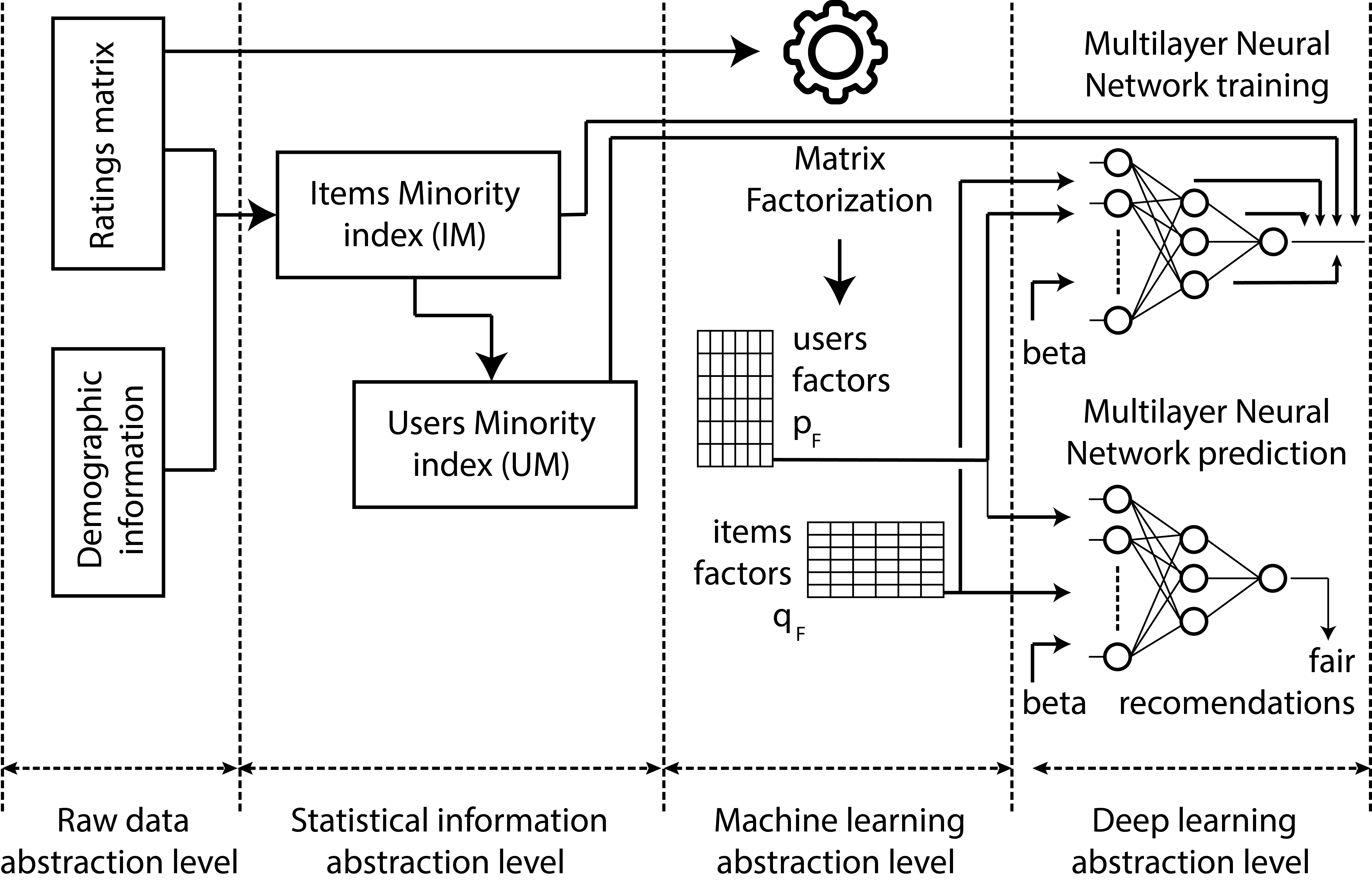
Figure 1. Architecture overview.

We will develop each of the three levels that make up our architecture: first, in the lowest level we create two related indexes: 1) items minority index (IM), and 2) users minority index (UM). The IM index will assign a minority value to each item in the dataset; e.g. when the minority group is ‘female’ we could call to the index ‘femininity’. It will contain values ($\left[-1,1\right]$) where negative ones mean feminine preferences and positive ones mean masculine preferences. Then, when an item has been assigned a negative value it means that it has been rated better by women than men. Once the IM index has been created it contains the minority values of all the items. By using the IM index, we will create the UM index. The UM index will assign a minority value to each user in the dataset. It also will contain values ($\left[-1,1\right]$), where negative ones mean minority preferences and positive ones mean not minority preferences (masculine, in our example). A user assigned a negative UM value means that this user prefers negative IM items, and vice versa. Please note that, on many occasions, female users may have assigned positive UM values and male users may have assigned negative UM values, since there exist women with masculine preferences and men with feminine ones; same as young and older persons or any other minority versus majority groups. Thus, an important concept is that both the IM and UM indexes do not contain disjoint minority/majority demographic values; they contain minority/majority preferences. This design accurately fits the existing diversity of preferences contained in the CF based RS.

Now, we will explain the IM and UM indexes design that we will take as a base to get fair recommendations in the DL stage. First, we will differentiate between relevant and not relevant votes: relevant votes are those that indicate that the user liked the item; conversely not relevant votes (in our context) are those that indicate that the user did not liked the item. They can also exist votes that indicate indifference on the part of the user. In our formulation, relevant and not relevant votes are chosen by means of two thresholds; e.g. in a dataset where votes must be in the set $\left\{1,2,3,4,5\right\}$ we can establish $4$ as the relevant threshold and $2$ as the non-relevant threshold. In this way the relevant set is $\left\{5,4\right\}$, the non-relevant set is $\left\{2,1\right\}$ and $\left\{3\right\}$ would be the ‘indifference’ set.

We define the IM index (equation 11) for each item $i$ as the majority score of $i$ minus the minority score of $i$. The majority score (resp. minority score) of the item $i$ is the number of majority (resp. minority) users that voted $i$ as relevant minus the number of majority (resp. minority) users that voted $i$ as non-relevant, divided by the total amount of majority (resp. minority) users that did not consider $i$ as indifferent, see equations 9 and 10 (resp. equations 7 and 8). When the proportion of the minority user preferences exceeds the proportion of the non-minority ones, the IM index values are negative. In the gender example, equation 11 can be read as: “proportion of males that liked item $i$ minus males that did not like it, minus the proportion of females that liked item $i$ minus females that did not like it”. We have also set a minimum number of $5$ votes to consider both the minority and non-minority sides of equation 11.

Once the IM index has been created, we can use it to establish the UM index values. Each UM value corresponds to a user of the RS dataset, and it provides the minority value of the user. Each user minority value will be defined by the minority of his/her preferences: to obtain each user UM value we just make the average of the IM minority values of the items that the user has voted, weighting each IM minority value with its corresponding user rating. LABEL:eq:um-index models the explained behaviour.

(1) Let $$\Theta_{\uparrow}\text{ be the like threshold}$$

(2) Let $$\Theta_{\downarrow}\text{ be the dislike threshold}$$

(3) Let $$I\text{ be the set of items in the dataset}$$

(4) Let $$U\text{ be the set of users in the dataset}$$

We will assign the following meanings to super index numbers, $m$ for minority and $M$ for non-minority:

(5) Let $$U^{m}\text{ be the set of minority users}$$

(6) Let $$U^{M}\text{ be the set of non-minority users}$$

(7) Let $$U_{\uparrow}(i)=\left\{u\in U|r_{u,i}\geq\Theta_{\uparrow}\right\}\text{ be the set of users who liked item }i$$

(8) Let $$U_{\downarrow}(i)=\left\{u\in U|r_{u,i}\leq\Theta_{\downarrow}\right\}\text{ be the set of users who did not like item }i$$

The majority score is

(9) $$\mathfrak{I}^{M}(i)=\frac{|U_{\uparrow}(i)\cap U^{M}|-|U_{\downarrow}(i)\cap U^{M}|}{|U_{\uparrow}(i)\cap U^{M}|+|U_{\downarrow}(i)\cap U^{M}|}$$

The minority score is

(10) $$\mathfrak{I}^{m}(i)=\frac{|U_{\uparrow}(i)\cap U^{m}|-|U_{\downarrow}(i)\cap U^{m}|}{|U_{\uparrow}(i)\cap U^{m}|+|U_{\downarrow}(i)\cap U^{m}|}$$

The IM and UM indexes are

(11) $$IM(i)=\mathfrak{I}^{M}-\mathfrak{I}^{m}$$

(12) $$IM=\left\{\left(i,IM(i)\right)|i\in I\right\}$$

(14) $$UM=\left\{\left(u,UM(u)\right)|u\in U\right\}$$

where $\circ$ means “not voted item” and $N$ is the maximum possible vote.

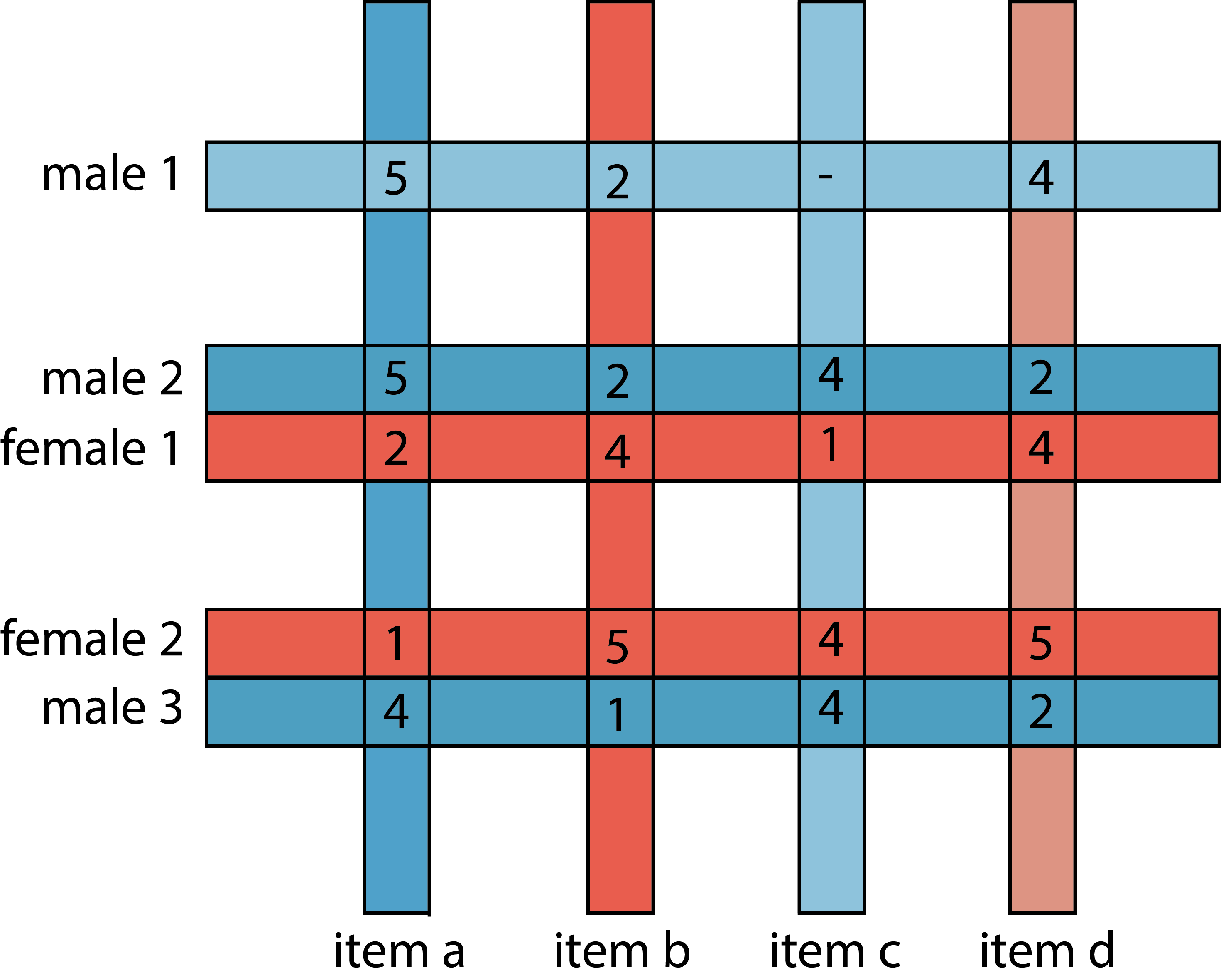
Figure 2. Data-toy example to get IM and UM minority values.

item	value
a	$[(3-0)-(0-2)]/5=1$
b	$[(0-3)-(2-0)]/5=-1$
c	$[(2-0)-(1-1)]/4=0.5$
d	$[(1-2)-(2-0)]/5=-0.6$

Figure 3. Data-toy IM results

Figure 3 shows a data-toy example containing five users and four items. We will suppose that women are a minority group in this RS, compared to the men. We can observe that ‘item a’ is clearly ‘masculine’, since it has been voted as ‘relevant’ for all the male users and it has been voted as ‘non-relevant’ for all the female users. The opposite situation is stated in ‘item b’: it is a ‘feminine’ item according to the female relevant votes and the male non-relevant ones. ‘Item c’ is quite masculine, although a female user liked it. Finally, ‘item d’ shows the opposite situation to ‘item c’. According to it, the proposed IM equations return the following item minority values:

$$\left\{\left\langle\text{item a},1\right\rangle,\left\langle\text{item b},-1\right\rangle,\left\langle\text{item c},0.5\right\rangle,\left\langle\text{item d},-0.6\right\rangle\right\}$$

that fits with the explained behaviour (Figure 3). Once the items’ minority values IM are obtained, we can get the users minority ones (UM). First, we can observe how ‘male 2’ and ‘male 3’ users in the data-toy example have casted very ‘masculine’ ratings, since they have voted ‘relevant’ to the more ‘masculine’ items, and ‘non-relevant’ to the more ‘feminine’ items. This is not the case for the ‘male 1’ user, that has a ‘relevant’ vote casted on the ‘feminine’ ‘item d’. The female users comparative is more complicated: ‘female 1’ has casted all her votes in a ‘feminine’ way, whereas the ‘female 2’ vote to the ‘masculine’ ‘item c’ was ‘relevant’; nevertheless, the ‘female 2’ feminine votes are higher than the ‘feminine 1’ ones. In this way, we expect the following results: a) positive UM values to male users and negative ones to female users, and b) a more ‘minority’ (feminine) value be assigned to ‘male 1’ than to ‘male 2’ and ‘male 3’. Figure 3 shows the Figure 3 data-toy IM results and Table 1 shows the UM ones.

user	value
male 1	$(5-3)\cdot 1+(2-3)\cdot(-1)+(4-3)\cdot(-0.6)=2.4/5=0.48$
male 2	$(5-3)\cdot 1+(2-3)\cdot(-1)+(4-3)\cdot 0.5+(2-3)\cdot(-0.6)=4.1/5=0.82$
female 1	$(2-3)\cdot 1+(4-3)\cdot(-1)+(1-3)\cdot 0.5+(4-3)\cdot(-0.6)=-3.6/5=-0.72$
female 2	$(1-3)\cdot 1+(5-3)\cdot(-1)+(4-3)\cdot 0.5+(5-3)\cdot(-0.6)=-4.7/5=-0.94$
male 3	$(4-3)\cdot 1+(1-3)\cdot(-1)+(4-3)\cdot 0.5+(2-3)\cdot(-0.6)=4.1/5=0.82$

Table 1. Data-toy UM results

Our architecture uses the PMF method to reduce the ratings matrix dimension and to get a condensed knowledge representation. From the condensed results we will be able to make accurate predictions. Equations 26 to 35 show the model formalization: the original ratings matrix is condensed in the two lower dimension matrices $P$ and $Q$ (equation 26). $P$ is the users’ matrix and $Q$ is the items’ matrix. Both $P$ and $Q$ have a common dimension of $F$ hidden factors, where $F\ll M$ and $F\ll M$ (note that $M$ is numbers of users, and $N$ the number of items). Once the model has learnt, each user will be represented by a vector $\vec{p}_{u}$ of $F$ factors, and each item will be also represented by a vector $\vec{q}_{i}$ of $F$ factors. Each prediction of an item $u$ to a user $i$ is obtained by processing the dot product of these vectors (equation 27). Since the users and the items hidden factors share the same semantic, predictions will be relevant when high values (positive or negative) of the factors line up in each user and item.

(26) $$R\approx\hat{R}=P\cdot Q^{t}$$

(27) $$\hat{r}_{u,i}=\vec{p}_{u}\cdot\vec{q}_{i}=\sum_{f=1}^{F}p_{u,f}\cdot q_{i,f}$$

The $P$ and $Q$ factors will be used in our architecture to feed the DL process input as well as to set the output target labels. Factors are obtained by means of the gradient descent algorithm. The loss function just minimizes the prediction error: the difference between the predicted value and the existing rating (equation 28).

(28) $$\mathrm{loss}(u,i)=\left(r_{u,i}-\hat{r}_{u,i}\right)^{2}$$

In order to achieve the gradient descent minimization process we obtain the partial loss derivatives: $\delta\mathrm{loss}/\delta\vec{p}_{u}$ and $\delta\mathrm{loss}/\delta\vec{q}_{i}$ (equations 29 and 30).

(29) $$\frac{\delta\mathrm{loss}}{\delta\vec{p}_{u}}=\frac{\delta}{\delta\vec{p}_{u}}\left(r_{u,i}-\vec{p}_{u}\cdot\vec{q}_{i}\right)^{2}=-2\vec{q}_{i}\cdot\left(r_{u,i}-\vec{p}_{u}\cdot\vec{q}_{i}\right)=-2\vec{q}_{i}\cdot e_{u,i}$$

(30) $$\frac{\delta\mathrm{loss}}{\delta\vec{q}_{i}}=\frac{\delta}{\delta\vec{q}_{i}}\left(r_{u,i}-\vec{p}_{u}\cdot\vec{q}_{i}\right)^{2}=-2\vec{p}_{u}\cdot\left(r_{u,i}-\vec{p}_{u}\cdot\vec{q}_{i}\right)=-2\vec{p}_{u}\cdot e_{u,i}$$

This gives rise to the corresponding gradient descent factors update Equations 31 and 32.

(31) $$\acute{p}_{u,f}=p_{u,f}+2\gamma\cdot q_{f,i}\cdot e_{u,i}$$

(32) $$\acute{q}_{f,i}=q_{f,i}+2\gamma\cdot p_{q,f}\cdot e_{u,i}$$

Finally, we can add a regularization term for controlling the growing of the factors during the learning process, which gives rise to the loss function and the update rules shown in Equations 33 to 35.

(33) $$\mathrm{loss}(u,i)=\left(r_{u,i}-\hat{r}_{u,i}\right)^{2}+\frac{\lambda}{2}\sum_{f=1}^{F}\left(\left\|P^{2}\right\|+\left\|Q^{2}\right\|\right)$$

(34) $$\acute{p}_{u,f}=p_{u,f}+\gamma\left(2q_{f,i}\cdot e_{u,i}-\lambda\cdot p_{uf}\right)$$

(35) $$\acute{q}_{f,i}=q_{f,i}+\gamma\left(2p_{uf}\cdot e_{u,i}-\lambda\cdot q_{f,i}\right)$$

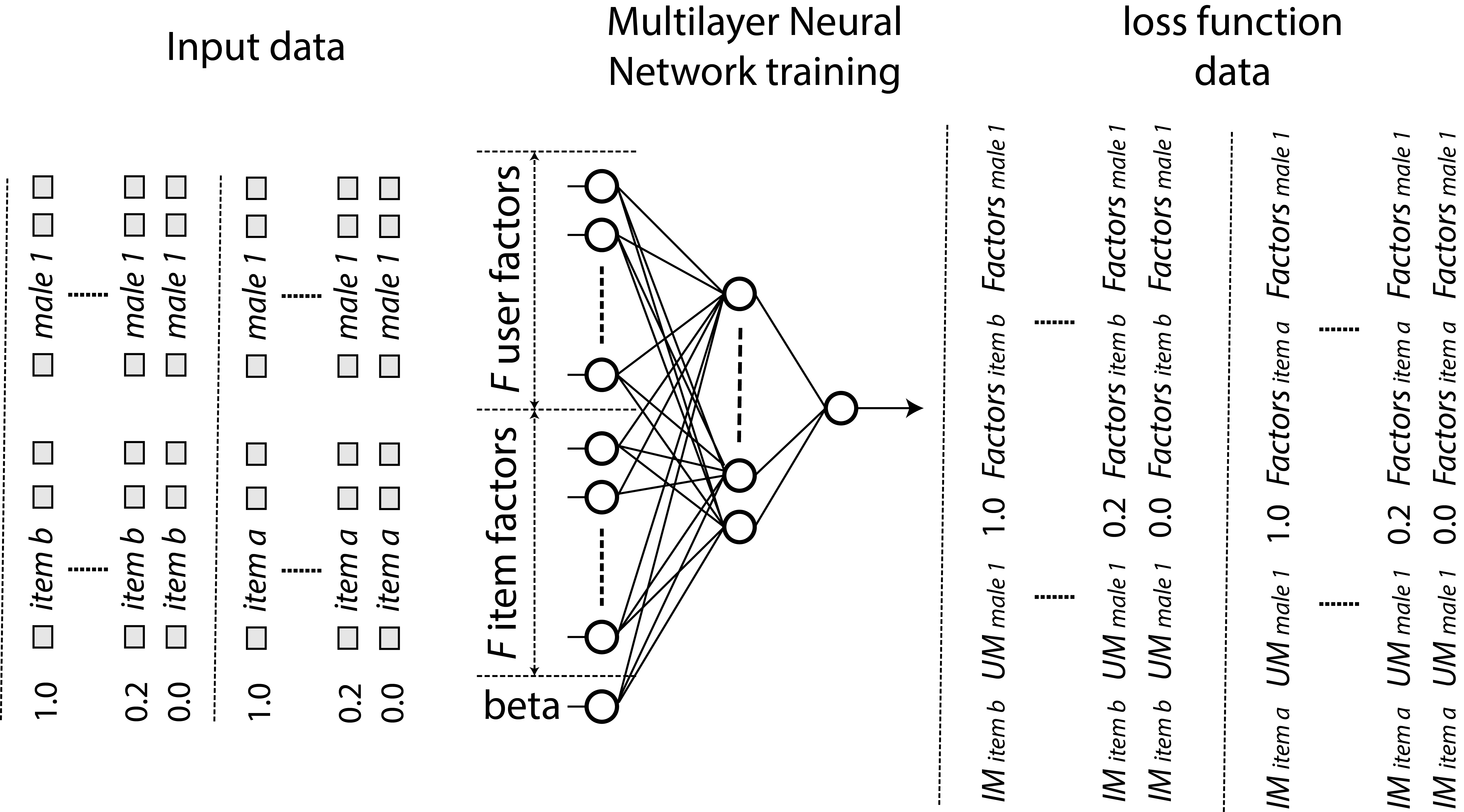
Figure 4. Training information for the proposed MLN.

The highest semantic level of the proposed architecture is based on an MLN. Our MLN (see figure 4) model will take input vectors containing the following information: a) user hidden factors $\vec{p}_{u}$, b) item hidden factors $\vec{q}_{i}$, and c) $\beta\in\left[0,1\right]$ value. The $\beta$ parameter is used to balance fairness and accuracy in predictions and recommendations: high $\beta$ values will enhance accuracy, whereas low $\beta$ values will enhance fairness. This balance is a key objective of our method: “To obtain fair recommendations just losing an acceptable degree of accuracy”. Please note that we do not include demographic information to feed the MLN input, so once the MLN has learnt it will be able to make fair recommendations to users that have not filled demographic forms asking for gender, age, etc. This is an important commercial advantage, since it allows to make better marketing processes, to improve fairness, to focus prediction tasks, etc. It is also a challenge to the proposed machine learning framework, because it is more difficult to increase recommendation fairness when demographic data is missing. The learning process has been based on input vectors containing the specified three information sources:$\left\langle p_{u,f},q_{f,i},\beta\right\rangle$ . We have set 11 input vectors to the MLN for each $\left\langle\text{user u},\text{item i}\right\rangle$ rating of the dataset:

$$\left\langle p_{u,f},q_{f,i},0.0\right\rangle,\left\langle p_{u,f},q_{f,i},0.2\right\rangle,\ldots,\left\langle p_{u,f},q_{f,i},1.0\right\rangle$$

The objective is to teach to the neural network on eleven fairness levels for each rating, as it can be seen in the left side of figure 4.

Once the MLN input vectors have been established, it is necessary to define their corresponding output labels in order to let the back propagation algorithm learn the pattern. In our case we will design a loss function that minimizes both the prediction error and the fairness error. Equation 36 shows the typical prediction loss function, as we did in equation 28. We define the fairness error as the distance between the user’s minority and the item’s minority; e.g. films recommended to a user (male or female) with an assigned $-0.8$ UM femininity value should be as similar as possible to a $-0.8$ IM in order to fit in the fairness issue. Since UM and IM vector values do not have the same distribution, we will apply a $\left[0,1\right]$ normalization in both of them and we will use the UM’ and IM’ names for the normalized versions. Then, to obtain the fairness error we establish equation 37. Finally, to combine equation 36 (accuracy) and equation 37 (fairness) the $\beta$ parameter is added (equation 38).

(36) $$e_{u,i}^{\mathrm{accuracy}}=\left(r_{u,i}-\sum_{f=0}^{F}p_{u,f}\cdot q_{i,f}\right)^{2}$$

(37) $$e_{u,i}^{\mathrm{fairness}}=\left(IM^{\prime}_{i}-UM^{\prime}_{u}\right)^{2}$$

(38) $$\mathrm{loss}_{u,i}=\beta\cdot e_{u,i}^{\mathrm{accuracy}}+\left(1-\beta\right)\cdot e_{u,i}^{\mathrm{fairness}}$$

In the feed forward prediction stage, for each testing input data $\left\langle p_{u,f},q_{f,i},\beta\right\rangle$, the proposed neural network returns a real number whose meaning is the predicted loss error for the item $i$ to the user $u$ recommendation. The lower the predicted loss error, the better the combined $\left\langle\mathrm{accuracy},\mathrm{fairness}\right\rangle$ values given the chosen $\beta$ accuracy vs. fairness balance. Once the network has learnt and the RS is in production phase, to make recommendations to an active user $u$, first we fix the $\beta$ value and then we feed the MLN with all the inputs $\left\langle\vec{p}_{u},\vec{q}_{i},\beta\right\rangle$ where $i$ runs over the set of items that the user $u$ has not voted (equation 39).

(39) $$X=\left\{\left\langle p_{u,f},q_{f,i},\beta\right\rangle\Big{|}u\in U,i\in I,r_{u,i}\neq\circ\right\}$$

The set of $N$ recommendations for the user $u$, $Z_{u,N}$ is the collection of $N$ items with minimum loss function $h(\vec{p}_{u},\vec{q}_{i},\beta)$, where the $h$ function represents the MLN feed forward operation.

Experiments have been conducted using a well known dataset called MovieLens 1M [14]. It contains 1,209,000 votes, 6040 users and 3952 items. We have used eleven different values of the $\beta$ parameter (from 0.0 to 1.0, step 0.2); consequently, the MLN has been trained using 13,299,000 input vectors and output target values. Training, validation and test sets have been established: 70%, 10% and 20%, respectively. The PMF process has been run using 30 hidden factors ($F$), 80% training ratings, 20% testing ratings. Please note that these are the MLN parameters of the proposed method, different to the previously ones specified for the DL stage. The designed MLN contains an input layer of $30+30+1=61$ values (figure 4). The first MLN internal layer has been set to 80 neurons (relu activation), followed by a 0.2 dropout layer to avoid overfitting. The second internal layer has been set to 10 neurons (relu activation) and, finally, the output layer contains just one neuron with no activation function. The chosen loss function has been mae and the optimizer rmsprop.

4. Results

The experiments we have conducted are:

• Item Minority Index (IM) and User Minority Index (UM) distributions.

• User Minority Index (UM) comparative between each minority and non-minority group.

• Fairness prediction improvement using the heuristic algorithm.

• Fairness recommendation improvement using the heuristic algorithm.

• Fairness error and accuracy error for recommendations using the proposed DL architecture.

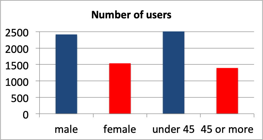
Figure 5. Proportion of users in the MovieLens gender and age minority and non-minority groups.

This section contains a subsection for each of the above set of performed experiments. We have selected two types of minority sets: a) gender: female vs. male, and b) youth: young vs. senior. Results are provided showing both minority types in two separated graphs of each figure. The MovieLens dataset, like in many other CF RS happens, is biased towards female and young people. Thus, the chosen minority types are relevant and representative for this experimental study. Specifically, the MovieLens dataset contains more males than females; most of them are under 45 years old. Figure 5 shows the proportions.

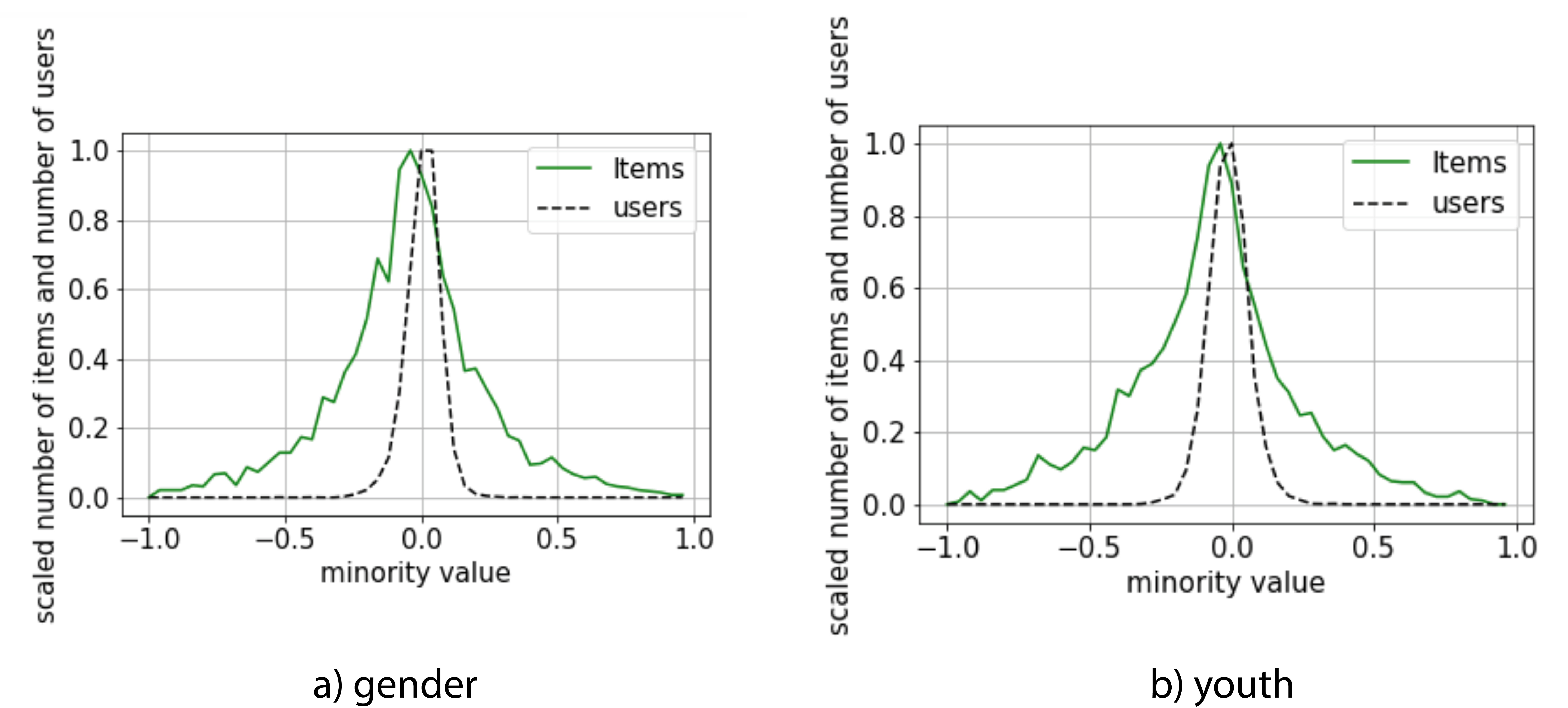
Figure 6. Item Minority Index (IM) and User Minority Index (UM) distributions.

Equations 11 and LABEL:eq:um-index describe both indexes behaviour. The IM index semantic is simple and convincing, but it is necessary to be aware that we are not working with absolute values: in order to prevent data biases and to maintain the index values in a bounded range, we are working with preferences proportions; e.g. “proportion of male users that liked the items minus proportion of female users that liked the item”. Since we expect a significant number of items that both minority and non-minority groups simultaneously like or dislike, IM proportions will be similar for both groups and consequently a significant number of IM values will concentrate around the 0.0 value. Figure 6 shows the items and users minority indexes distributions, both for the gender and the youth minority groups.

The UM index values are obtained from the ratings that each user has casted to the items and from the IM value of each of those items. We can see in figure 6 that the users UM indexes (both for gender and youth) have a large concentration of values around 0. It provides us an important conclusion: “In the reference dataset, most users have similar preferences regarding to the chosen minority groups”. Looking at the UM distributions we can also yield another main conclusion: “Although users have similar preferences, there is a clear separation between minority groups” (left and right side of the graphs). Since the UM index is only used to feed internal DL processes the relevant information here is the proportion of the differences between values, and not their absolute values.

4.1. User Minority Index (UM) comparative between each minority and non-minority group

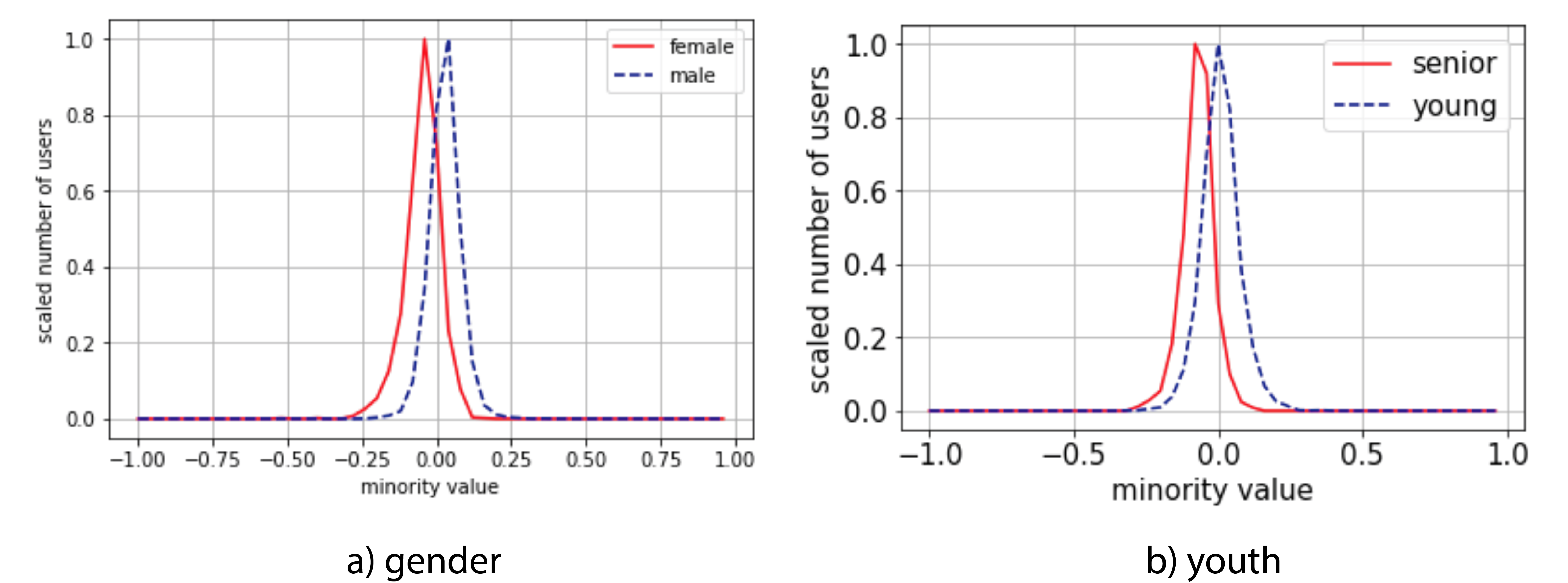
Figure 7. User Minority Index (UM) comparative.

In the above section we have confirmed two facts: 1) Users preferences are similar, even if they belong to different minority groups, and 2) Despite the previous conclusion, there is room to find minority behaviours of users. In this section we deepen in the minority UM values of users, to clear out our specific groups: male vs. female and senior vs. young. Figure 7 shows the results: we can observe, in both cases, that groups have different behaviours and also that they share a relevant number of preferences. Groups present different behaviours because they do not completely intersect their user minority values; as expected, minority groups return a mean less than zero whereas non-minority groups return it greater than zero. Groups share a relevant number of preferences because there exist a proportion of minority and non-minority users that share UM values (areas around 0.0 under both curves).

group	type	correct	incorrect	correct%
gender	female	1147	562	67.11
	male	3648	683	84.22
youth	senior	1231	195	86.32
	young	3144	1470	68.14

Table 2. Users classification attending to the minority/non-minority groups.

Due to the explained results, we can confirm that there is a not negligible proportion of minority users with non-minority preferences and vice versa. In any case, it varies depending on the specific minority group. As an example, we can observe in figure 7 how senior users have much less non-minority preferences than female ones, since there are small amounts of senior users whose minority value is greater than zero. Results show the convenience of using modern machine learning approaches to make fair recommendations to those users that share minority and non-minority preferences. Table 2 shows the specific number of users that have been classified as belonging to the minority or to the non-minority groups. Minority users (female, young) have an expected UM index less than zero. Non-minority users (male, senior) have an expected UM index greater than zero.

4.2. Fairness prediction improvement using a heuristic algorithm

	female	male	senior	young
IM mean	-0.014	0.041	-0.025	0.028

Table 3. Averaged IM values for the predictions made to each users’ group

Figure 7 and table 3 show us that the majority of the users are correctly grouped attending to their UM indexes, especially for seniors and males. They also show a considerable number of cases incorrectly classified, particularly for young and female groups. In this situation, we will obtain predictions from the test set and then check their quality in terms of the IM index. Table 3 contains these experiments results: the IM averages fit the expected ranges (negative IM average for minority users, and positive IM average for non-minority users). Despite these positive results, ranges can be too narrow to ensure fair predictions. On the other hand, there will be situations in which it is intended to force the recommendations of an RS to move towards minority items, or perhaps towards majority items, depending on the type of users and/or the company policy.

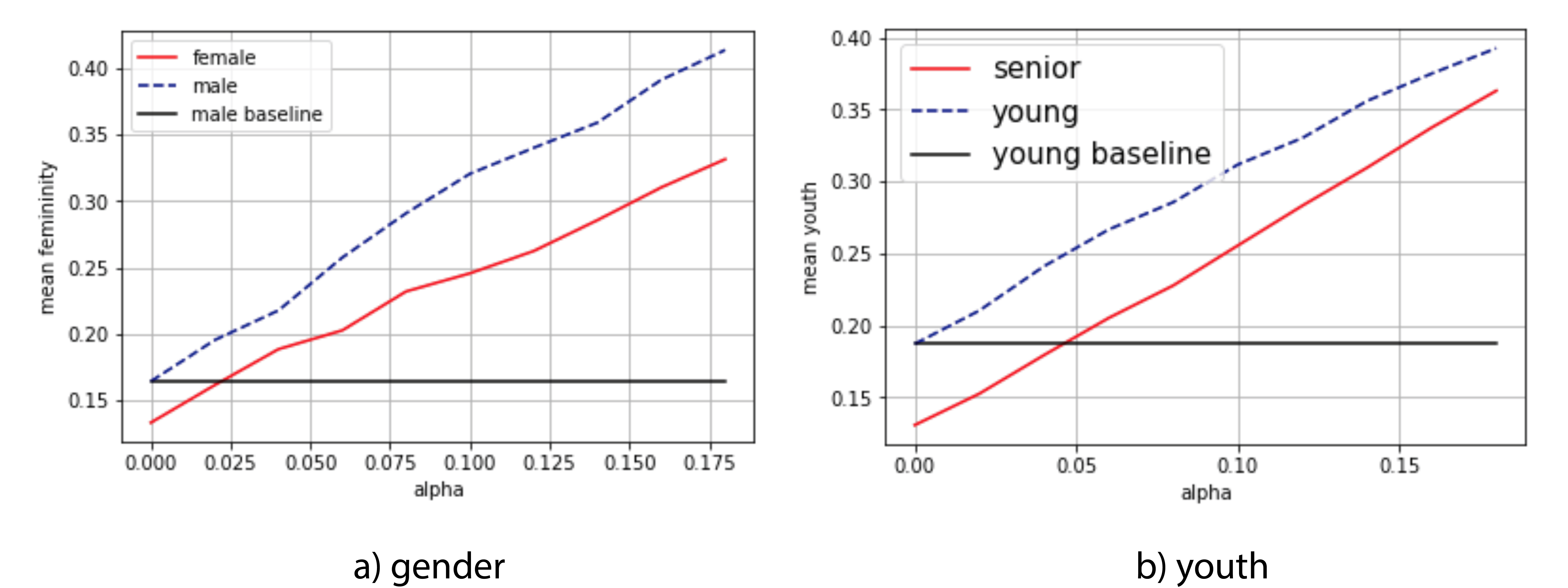
Figure 8. Groups quality improvement by filtering predictions. x axis: alpha values used to filter on the IM items index. y axis: averaged minority of the filtered predictions. Minority (female, senior) curves are drawn using their absolute values.

By filtering on the IM index, we can discard those predictions greater than a negative threshold and, in this way, increase the proportion of minority predictions. In the same way we can filter those predictions less than a positive threshold to increase the proportion of majority predictions. We have performed this experiment, calling alpha to the threshold. We can observe the expected behaviour in figure 8, where growing minority (and majority) IM values are obtained in predictions when the alpha parameter increases. It also can be seen that the non-minority users (male, young) always obtain better predictions due to the RS datasets biases. Finally, we can state that, in this case, minority values can reach the starting majority ones by using low values of the alpha parameter (0.025 for gender and 0.05 for age).

4.3. Fairness recommendation improvement using the heuristic algorithm

The previous section results show that it is possible to provide a heuristic method to improve recommendations fairness. To conduct the experiment, from the alpha filtered predictions (Figure 8), we extract the $N$ ones that provide higher prediction values, as usual in the CF operation. Thus, the complete recommendation method involves three sequential phases: 1) to obtain all the $\left\langle\text{prediction value},\text{minority value}\right\rangle$ pairs, 2) to filter the pairs according to the minority threshold alpha parameter and each minority value, and 3) to select the $N$ filtered predictions that have the $N$ highest prediction value values.

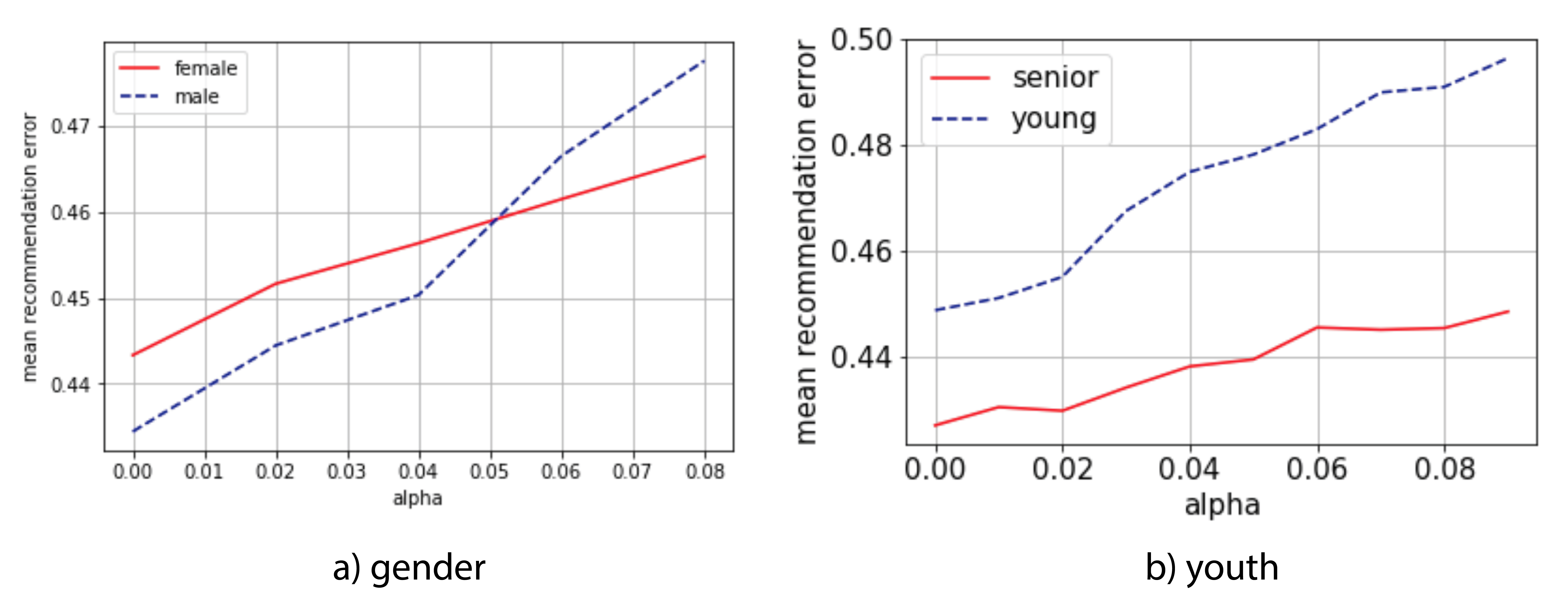
Figure 9. Recommendation quality obtained by filtering predictions. x axis: alpha values used to filter on the IM items index. y axis: averaged error of the $N$ recommendations. Lower error values are the better ones.

Results in figure 9 show the existing correlation between recommendation errors and each chosen alpha value: the highest the alpha value, the better the recommendations fairness (Figure 8), but as expected, also the worst the recommendation accuracy (higher error values in figure 9). Of course, we pay an accuracy price when we force fairer recommendations.

We have chosen a value of $N=10$ recommendations to process the set of experiments. From figure 8 it can be observed that in the ‘youth’ experiment our method provides better results (lower errors) for the minority ‘senior’ group than for the ‘young’ one. This is a good indication of the proposed heuristic method functioning. The ‘gender’ experiments provide improvement in the minority female group from a specific value threshold ($\mathrm{alpha}=0.05$). All these results are consistent with Tables 1 and 2 values.

4.4. Fairness error and accuracy error for recommendations using the proposed DL architecture

Results obtained in the previous subsection tell us that we have designed a method that correctly provides fair recommendations. It is a simple, functional and easy to implement machine learning approach. Nevertheless, it has some drawbacks:

• Choosing the adequate parameter alpha requires a fine-tuning process.

• Since the parameter alpha sign (less than or greater than zero) depends on the minority or non-minority nature of the recommended user, this recommendation method can only be applied to users with associated demographic information.

This subsection provides a DL approach that works without the above drawbacks. This method only needs the parameter $\beta$: it is used to select the accuracy vs. fairness balance. The $\beta$ range is $\left[0,1\right]$, whether 0 means 100% fairness and 0% accuracy, and 1 means 100% accuracy and 0% fairness. As it can be seen, to choose a $\beta$ value is straightforward and intuitive. Moreover: the chosen $\beta$ value does not change when the user is a minority one or he is not.

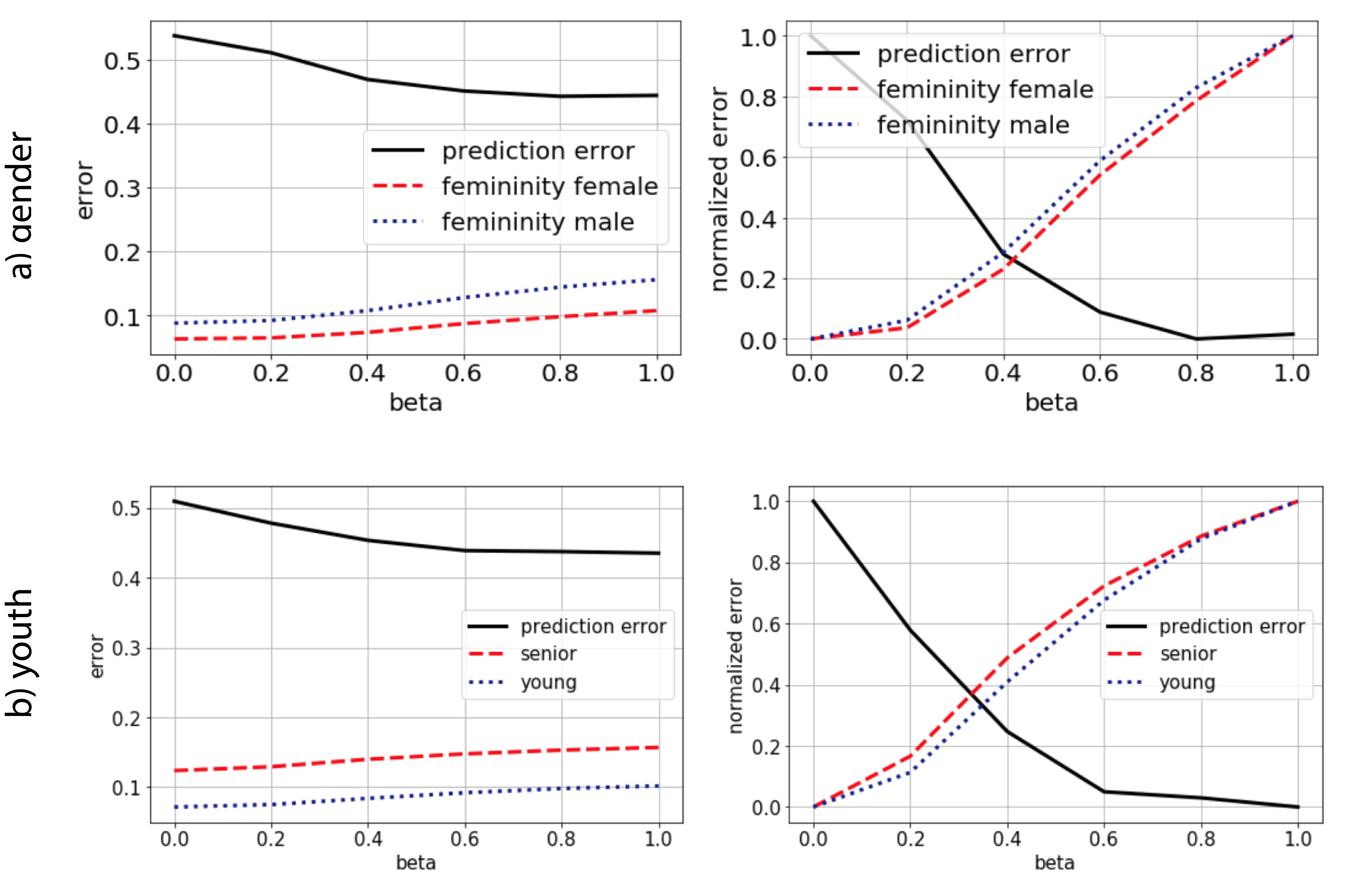
Figure 10. Recommendation results using the proposed DL approach. y axis: averaged $N=10$ recommendations error (normalized in the right graphs); x axis: $\beta$ balance between fairness and accuracy (0.0 means 100% fairness and 0% accuracy, and 1.0 means 100% accuracy and 0% fairness).

The proposed DL recommendation method explained in section 3 returns the results shown in figure 10. Graphs on the left of the figure contain the main information. Graphs on the right are $\left[0,1\right]$ scaled to find the optimum accuracy vs. fairness balances. The averaged error of the recommendations (equation 36) is plotted using black lines. Dotted and dashed lines show the minority errors (equation 37); that is: the distance between the minority value of each recommended user (UM) and the average of the minority values (IM) of their N recommended items. We are looking for recommended items in the minority range of the user; e.g. if a user (male or female) has an $UM=0.7$ (quite masculine), recommended items near $IM=0.7$ are the fairest ones, and they generate a low minority (‘femininity’) error.

‘Gender’ results are shown in the top-left graph of figure 10: as expected, accuracy increases (error decreases) as $\beta$ increases (more importance to accuracy). The price to pay for this accuracy improvement is the simultaneous increase in the fairness error values. As $\beta$ decreases (more importance to fairness), the opposite happens: higher prediction errors and lower fairness errors. ‘Youth’ results are shown in the low-left graph of figure 9: curve trends are similar to the ‘gender’ results. Graphs on the right of figure 9 show the same results by using a normalized y axis: in this way we can find the optimum $\beta$ values to balance accuracy and fairness in the recommendation task. To optimize results in this experiment, it is necessary to choose a $\beta=0.4$ value: a balanced selection, something scored to the fairness objective. This result tells us that the balanced option ($\beta=0.5$) can be the default one.

5. Conclusions

Attending to the obtained results, it is understood that designing methods to improve CF fairness is not a simple task, but it is possible to take it out. Due to the fact that an appreciable proportion of minority and non-minority users share preferences it is necessary to make use of modern machine learning approaches in order to make fair recommendations not only to the ‘purest’ minority or non-minority users, but also to the users that mix some proportion of minority and non-minority preferences.

State of the art shows a lack of DL approaches to tackle fairness in RS, probably due to the neural networks black box model. The proposed method in this paper relies on an original loss function and input data to balance fairness and accuracy. This method combines several abstraction levels and it can serve as baseline to DL future works in the field. An original architecture is provided, where machine learning and DL models are combined to obtain balanced accuracy vs. fairness recommendations. The architecture is based on two basement levels: statistical and machine learning, that provide the necessary information to train the DL model which constitutes the third architectural level. The proposed DL method provides a modern approach to tackle fairness in RS. We can easily balance accuracy and fairness, or we can automatically select the optimum trade-off. That is to say: the proposed method manages the inherent loss of accuracy when fairness is increased. Additionally, once the neural network is trained using demographic information, it can predict and recommend to users whose demographic information is unknown.

Results show adequate trends in the tested quality measures: improvement in fairness at the cost of an expected worsening in accuracy. The proposed machine learning-based heuristic approach and the DL model return similar quality results. Nevertheless, the proposed DL method does not need demographic information in the recommendation feed-forward process. It also is able to better balance and automatically balance fairness and accuracy.

Proposed future works are: a) architecture simplification, by removing the MF and transferring its functionality to the DL model, b) items and users minority indexes redefinition to better catch the minority versus non-minority differences, c) testing the methods behaviour in a variety of CF datasets, d) extending the experiments to different demographic groups (nationality, profession, studies), and e) testing the architecture on not demographic groups (users that share minority preferences).

References

- [1] Z. Batmaz, A. Yurekli, A. Bilge, and C. Kaleli. A review on deep learning for recommender systems: challenges and remedies. Artificial Intelligence Review, 52(1):1–37, June 2019.
- [2] A. Bellogín, P. Castells, and I. Cantador. Statistical biases in Information Retrieval metrics for recommender systems. Information Retrieval Journal, 20(6):606–634, Dec. 2017.
- [3] J. Bobadilla, S. Alonso, and A. Hernando. Deep Learning Architecture for Collaborative Filtering Recommender Systems. Applied Sciences, 10(7):2441, Jan. 2020.
- [4] J. Bobadilla, A. Gutiérrez, F. Ortega, and B. Zhu. Reliability quality measures for recommender systems. Information Sciences, 442-443:145–157, May 2018.
- [5] J. Bobadilla, F. Ortega, A. Gutiérrez, and S. Alonso. Classification-based deep neural network architecture for collaborative filtering recommender systems. International Journal of Interactive Multimedia and Artificial Intelligence, 6(1):68–77, Mar. 2020.
- [6] R. Burke, N. Sonboli, and A. Ordonez-Gauger. Balanced neighborhoods for multi-sided fairness in recommendation. In S. A. Friedler and C. Wilson, editors, Proceedings of the 1st Conference on Fairness, Accountability and Transparency, volume 81 of Proceedings of Machine Learning Research, pages 202–214, New York, NY, USA, 23–24 Feb 2018. PMLR.
- [7] E. Çano and M. Morisio. Hybrid recommender systems: A systematic literature review. Intelligent Data Analysis, 21(6):1487–1524, Jan. 2017.
- [8] J. Choo and S. Liu. Visual Analytics for Explainable Deep Learning. IEEE Computer Graphics and Applications, 38(4):84–92, July 2018.
- [9] A. Chouldechova and A. Roth. The frontiers of fairness in machine learning. CoRR, abs/1810.08810, 2018.
- [10] M. de Gemmis, P. Lops, G. Semeraro, and C. Musto. An investigation on the serendipity problem in recommender systems. Information Processing & Management, 51(5):695–717, Sept. 2015.
- [11] M. D. Ekstrand, M. Tian, M. R. I. Kazi, H. Mehrpouyan, and D. Kluver. Exploring author gender in book rating and recommendation. In Proceedings of the 12th ACM Conference on Recommender Systems, RecSys ’18, pages 242–250, New York, NY, USA, 2018. Association for Computing Machinery.
- [12] M. Fatehkia, R. Kashyap, and I. Weber. Using Facebook ad data to track the global digital gender gap. World Development, 107:189–209, July 2018.
- [13] R. Gao and C. Shah. Toward creating a fairer ranking in search engine results. Information Processing & Management, 57(1):102138, Jan. 2020.
- [14] F. M. Harper and J. A. Konstan. The movielens datasets: History and context. ACM Trans. Interact. Intell. Syst., 5(4), Dec. 2015.
- [15] X. He, L. Liao, H. Zhang, L. Nie, X. Hu, and T.-S. Chua. Neural collaborative filtering. In Proceedings of the 26th International Conference on World Wide Web, WWW ’17, pages 173–182, Republic and Canton of Geneva, CHE, 2017. International World Wide Web Conferences Steering Committee.
- [16] J. L. Herlocker, J. A. Konstan, L. G. Terveen, and J. T. Riedl. Evaluating collaborative filtering recommender systems. ACM Transactions on Information Systems, 22(1):5–53, Jan. 2004.
- [17] A. Hernando, J. Bobadilla, and F. Ortega. A non negative matrix factorization for collaborative filtering recommender systems based on a Bayesian probabilistic model. Knowledge-Based Systems, 97:188–202, Apr. 2016.
- [18] K. Holstein, J. Wortman Vaughan, H. Daumé, M. Dudik, and H. Wallach. Improving fairness in machine learning systems: What do industry practitioners need? In Proceedings of the 2019 CHI Conference on Human Factors in Computing Systems, CHI ’19, New York, NY, USA, 2019. Association for Computing Machinery.
- [19] D. Kotkov, S. Wang, and J. Veijalainen. A survey of serendipity in recommender systems. Knowledge-Based Systems, 111:180–192, Nov. 2016.
- [20] M. Kunaver and T. Požrl. Diversity in recommender systems – A survey. Knowledge-Based Systems, 123:154–162, May 2017.
- [21] J. Leonhardt, A. Anand, and M. Khosla. User fairness in recommender systems. In Companion Proceedings of the The Web Conference 2018, WWW ’18, pages 101–102, Republic and Canton of Geneva, CHE, 2018. International World Wide Web Conferences Steering Committee.
- [22] M. Mansoury, B. Mobasher, R. Burke, and M. Pechenizkiy. Bias Disparity in Collaborative Recommendation: Algorithmic Evaluation and Comparison. ArXiv e-prints, Aug. 2019.
- [23] N. Mehrabi, F. Morstatter, N. Saxena, K. Lerman, and A. Galstyan. A survey on bias and fairness in machine learning, 2019.
- [24] R. Mehrotra, J. McInerney, H. Bouchard, M. Lalmas, and F. Diaz. Towards a fair marketplace: Counterfactual evaluation of the trade-off between relevance, fairness & satisfaction in recommendation systems. In Proceedings of the 27th ACM International Conference on Information and Knowledge Management, CIKM ’18, pages 2243–2251, New York, NY, USA, 2018. Association for Computing Machinery.
- [25] M. Mendoza and N. Torres. Evaluating content novelty in recommender systems. Journal of Intelligent Information Systems, 54(2):297–316, Apr. 2020.
- [26] R. Mu. A Survey of Recommender Systems Based on Deep Learning. IEEE Access, 6:69009–69022, Nov. 2018.
- [27] I. Portugal, P. Alencar, and D. Cowan. The use of machine learning algorithms in recommender systems: A systematic review. Expert Systems with Applications, 97:205–227, May 2018.
- [28] N. S. Santos, A. García-Holgado, and M. C. Sánchez-Gómez. Gender gap in the digital society: A qualitative analysis of the international conversation in the wyred project. In Proceedings of the Seventh International Conference on Technological Ecosystems for Enhancing Multiculturality, TEEM’19, pages 518–524, New York, NY, USA, 2019. Association for Computing Machinery.
- [29] V. Tsintzou, E. Pitoura, and P. Tsaparas. Bias disparity in recommendation systems. CoRR, abs/1811.01461, 2018.
- [30] H. Wu, Z. Zhang, K. Yue, B. Zhang, J. He, and L. Sun. Dual-regularized matrix factorization with deep neural networks for recommender systems. Knowledge-Based Systems, 145:46–58, Apr. 2018.
- [31] S. Yao and B. Huang. Beyond parity: Fairness objectives for collaborative filtering. CoRR, abs/1705.08804, 2017.