A one-dimensional model for elasto-capillary necking

Abstract

We derive a non-linear one-dimensional (1d) strain gradient model predicting the necking of soft elastic cylinders driven by surface tension, starting from 3d finite-strain elasticity. It is asymptotically correct: the microscopic displacement is identified by an energy method. The 1d model can predict the bifurcations occurring in the solutions of the 3d elasticity problem when the surface tension is increased, leading to a localization phenomenon akin to phase separation. Comparisons with finite-element simulations reveal that the 1d model resolves the interface separating two phases accurately, including well into the localized regime, and that it has a vastly larger domain of validity than 1d model proposed so far.

1 Introduction

We consider a phase separation phenomenon occurring in very soft elastic cylinders immersed in a fluid. This phenomenon, first reported in Mora et al. (2010), is shown in figure 1. It is driven by surface tension, and is the elastic analogue of the Rayleigh-Plateau instability in fluids. It has been analyzed based on a linear bifurcation analysis (Mora et al., 2010) and, more recently, on weakly non-linear bifurcation analyses and on non-linear finite-element simulations (Taffetani and Ciarletta, 2015a; Xuan and Biggins, 2017). Here, we derive a one-dimensional model that captures this phenomenon accurately, including deeply into the post-bifurcation regime.

Various localization phenomena occurring in non-linear slender structures have been analyzed recently based on one-dimensional models, including the necking of hyper-elastic or bars (Audoly and Hutchinson, 2016), the bulging in axisymmetric balloons (Lestringant and Audoly, 2018), or the folding of tape-springs (Martin et al., 2020; Brunetti et al., 2020). Even though different one-dimensional models have been proposed for each one of these phenomena, these models are all mathematically similar.

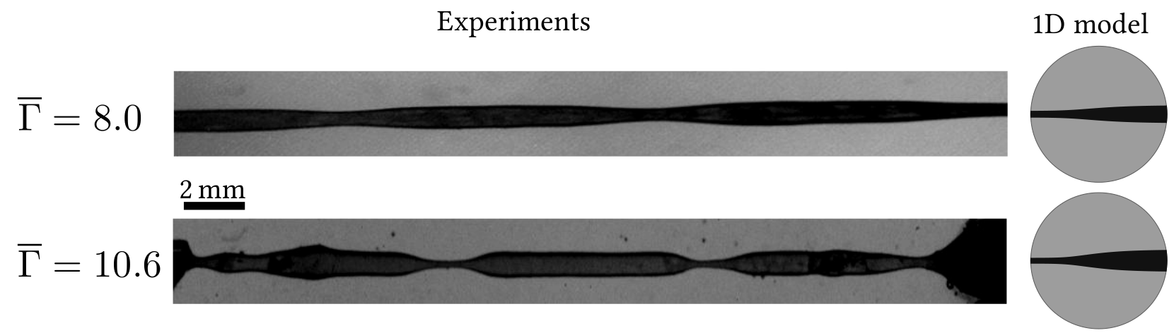
Figure 1: Equilibrium shapes of agar gel filaments with varying shear modulus $G$, fixed surface tension $\Gamma$ and undeformed radius $\rho$. The instability is controlled by the dimensionless parameter $\overline{\Gamma}=\Gamma/\,(\rho G)$ corresponding to the ratio of the elasto-capillary length to the cylinder’s radius; the critical value is $\overline{\Gamma}_{\mathrm{c}}\approx 5.7$. The aspect ratio of the filaments is $\epsilon=\rho/L\approx 0.012$. The profile of the interfaces between regions with constant radius is shown in the second column for the same set of parameters, as predicted by 1d strain gradient model derived in this paper. Experimental pictures courtesy of Serge Mora.

Like the diffuse-interface model of van der Waals (1894), they are built on a strain energy potential made up of a non-convex function of the elastic strain, plus a regularizing term function of the gradient of strain—these models will be generically referred to as strain gradient models. As is well known in the context of one-dimensional solid-solid phase separation (Ericksen, 1975; Carr et al., 1984), strain gradient models can account for localization phenomena: the non-convex energy tends to produce coexisting phases of constant strain while the regularizing term penalizes sharp variations of the strain, thereby accounting for the presence of diffuse interfaces between phases and for their energy.

One-dimensional (1d) models offer an efficient approach to localization phenomena and remove the need for complex and computationally costly simulations, such as the non-linear shell simulations that are traditionally used for the analysis of tape springs. This makes 1d models very attractive. However these models have often been derived from ad hoc kinematic assumptions (Xuan and Biggins, 2017; Martin et al., 2020): their accuracy is not well controlled and their domain of validity is unclear.

This work is part of an ongoing effort from the authors to derive 1d models for various non-linear slender structures, based on a systematic two-scales expansion method. The 1d models obtained in this way are asymptotically correct in the limit where the length-scale over which the strain varies is much larger than the transverse dimension of the structure, although in several cases they have been found to remain highly accurate in regions of large strain gradients. They also tend to be simpler than alternatives based on ad hoc kinematic assumptions, as discussed elsewhere (Audoly and Hutchinson, 2016; Lestringant and Audoly, 2018). In this paper, we apply the general reduction method which we proposed in Lestringant and Audoly (2020), to the case of an axisymmetric, hyper-elastic cylinder with surface tension; doing so, we obtain a non-linear one-dimensional strain gradient model that captures elasto-capillary necking. We compare its predictions to finite-element simulations of full three-dimensional (3d) model, and find good agreement, including deep in the post-bifurcation regime when the interfaces are well localized. This complements previous work on a 1d model for elastic necking without surface tension, where the comparison with the full 3d model was limited to the neighborhood of the bifurcation (Audoly and Hutchinson, 2016).

For cylinders made of very soft solids, the elasto-capillary length, defined as the ratio of the surface tension over the shear modulus, is comparable to the cylinder radius. In this regime, surface tension competes with elasticity, generating localized patterns akin to those produced by the Plateau-Rayleigh instability in fluids. This was experimentally demonstrated by Mora et al. (2010) in filaments of agar gel. By varying the shear modulus $G$ for a fixed surface tension $\Gamma$ and a fixed undeformed radius $\rho$, they showed that the dimensionless parameter $\overline{\Gamma}=\Gamma/(\rho\,G)$ determines the width of the interfaces, as illustrated in Figure 1. Using a linear stability analysis they found that the instability occurs when $\overline{\Gamma}$ exceeds a critical value $\overline{\Gamma}_{\text{c}}$. This instability has been further explored and characterized by Taffetani and Ciarletta (2015a); Taffetani and Ciarletta (2015b) using 3d finite elasticity theory combined with linear and weakly nonlinear bifurcation analysis and numerical simulations in the nonlinear regime. Recently, Xuan and Biggins (2017) revisited the elasto-capillary buckling as a phase separation process, and used Maxwell’s construction to predict the amplitude of the localization pattern. Based on a weakly non-linear analysis, they derived a 1d strain gradient model capturing the onset of localization, i.e., when $\overline{\Gamma}-\overline{\Gamma}_{\text{c}}\ll 1$.

In this paper, we extend the work of Xuan & Biggins and derive a 1d gradient model that is not limited to the onset of localization. Our model allows finite variations of the axial strain across the length of the cylinder, and does not assume the parameter $\overline{\Gamma}-\overline{\Gamma}_{\text{c}}$ to be small. It is asymptotically justified when the gradient of the axial strain is small compared to the inverse radius of the cylinder but remains highly accurate even when this assumption is not satisfied, i.e., in the presence of the sharp interfaces that arise for relatively large values of $\overline{\Gamma}/\overline{\Gamma}_{\text{c}}$.

2 Problem formulation and summary of the main result

2.1 Finite-elasticity problem in 3d

We consider a hyper-elastic cylinder with undeformed length $L$ and undeformed radius $\rho$. The aspect-ratio $\epsilon=\rho/L$ is assumed to be small, $\epsilon\ll 1$. The cylinder deforms in an axisymmetric way under the combined effect of a traction force applied at its two ends, and of surface tension of its lateral boundary; the surface tension is represented in the model by an energy $\Gamma$ per unit area of the lateral surface, measured in actual configuration. The cylinder is assumed to be homogeneous, and its elastic constitutive law to be transversely isotropic (this includes the case of an isotropic material as a particular case). With these assumptions, there exist solutions to the elasticity problem with surface tension, such that the cross-sections remain planar and perpendicular to the axis; note that these ‘fundamental’ solutions may however not be stable. We use the cylindrical coordinates $(T,\Theta,S)$ in the reference, undeformed configuration as Lagragian variables and we denote by $(\mathbf{d}_{S},\mathbf{d}_{T}(\Theta),\mathbf{d}_{\Theta}(\Theta))$ the corresponding moving orthonormal frame, as sketched in Figure 2(a).

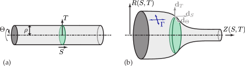
Figure 2: A hyper-elastic cylinder in (a) reference (undeformed) configuration and (b) actual configuration.

The current position of the point with Lagrangian coordinates $(T,\Theta,S)$ is $Z(S,T)\,\mathbf{d}_{S}+R(S,T)\,\mathbf{d}_{T}(\Theta)$, as shown in Figure 2(b). In axisymmetric geometry, the deformation gradient writes $\mathbf{F}=Z_{,S}\,\mathbf{d}_{S}\otimes\mathbf{d}_{S}+Z_{,T}\,\mathbf{d}_{S}\otimes\mathbf{d}_{T}+R_{,S}\,\mathbf{d}_{T}\otimes\mathbf{d}_{S}+R_{,T}\,\mathbf{d}_{T}\otimes\mathbf{d}_{T}+\frac{R}{T}\,\mathbf{d}_{\Theta}\otimes\mathbf{d}_{\Theta}$. The Green-Lagrange strain can then be calculated as

$$\mathbf{E}=\frac{1}{2}\left(\mathbf{F}^{T}\cdot\mathbf{F}-\mathbf{I}\right)=\frac{1}{2}\begin{pmatrix}Z_{,S}^{2}+R_{,S}^{2}-1&Z_{,S}Z_{,T}+R_{,S}R_{,T}&0\\ Z_{,S}Z_{,T}+R_{,S}R_{,T}&Z_{,T}^{2}+R_{,T}^{2}-1&0\\ 0&0&\left(\left(\frac{R}{T}\right)^{2}-1\right)\end{pmatrix}_{(S,T,\Theta)},$$ (1)

where the matrix notation provides the components of the tensor in the orthonormal local basis $(\mathbf{d}_{S},\mathbf{d}_{T}(\Theta),\mathbf{d}_{\Theta}(\Theta))$, as indicated by the label $(S,T,\Theta)$ in subscript of the matrix.

A model for the elastic material is specified through a strain energy potential $w(\mathbf{E})$; we work for the moment with a generic material model that is transversely symmetric with respect to the axis $Z$, and compressible. Later, we will focus on the special case of an incompressible neo-Hookean material.

The area magnification factor on the lateral surface is the quantity

$$J=\left.\frac{R}{T}\sqrt{Z_{,S}^{2}+R_{,S}^{2}}\right|_{T=\rho}\textrm{.}$$ (2)

The sum of the strain energy and the capillary energy of the system writes

$$\Phi_{\text{3d}}=\int_{0}^{L}\left(\int_{0}^{\rho}w(\mathbf{E})2\pi T\mathrm{d}T+\Gamma 2\pi\rho J\right)\mathrm{d}S.$$ (3)

The dimension reduction will be carried out on the potential $\Phi_{\text{3d}}$: the forces applied on the endpoints of the cylinder will be introduced later.

2.2 Dimension reduction strategy

With a view of conducting a dimension reduction procedure and thus reducing the kinematics of the system to a macroscopic apparent deformation, we define the average current coordinate $z(S)$ of the cross-section whose undeformed coordinate is $S$,

$$z(S)=\langle Z\rangle(S)=\frac{1}{\pi\rho^{2}}\int_{0}^{\rho}Z(S,T)\,2\pi T\,\mathrm{d}T,$$ (4)

where $\langle f\rangle$ denotes the average of a quantity $f$ over a cross-section. By construction, $z(S)$ is a function of the longitudinal coordinate $S$ only, see Figure 3(a); it will be the main kinematic variable of the 1d model. We define the apparent axial stretch ratio $\lambda(S)$ as $\lambda(S)=\frac{\mathrm{d}z}{\mathrm{d}S}$. The quantity $\lambda(S)$ with be the strain measure of our 1d model; it is apparent in the sense that $z(S)$ is an average position and not the coordinate of any material point.

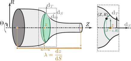
Figure 3: 3d kinematics in actual configuration. The macroscopic deformation is captured by the position $z(S)$ along the $Z$-axis of the center-of-mass of the cross-section with label $S$, while the detailed deformation in the cross-sections is fully described by the microscopic displacement $(Z(S,T)-z(S),R(S,T))$ (inset).

We focus on configurations of the cylinders such that typical scale of variation of $\lambda(S)$ is $L$: $\lambda(S)$ does not vary significantly on the scale $\rho\ll L$. In addition we allow finite variations of the stretch, $\lambda(S)=\mathcal{O}(1)$. With the convention that $L=\mathcal{O}(1/\epsilon)$ and $\rho=\mathcal{O}(1)$, this leads to the scaling assumption

$$\lambda(S)=\mathcal{O}(1),\quad\lambda^{\prime}(S)=\mathcal{O}(\epsilon),\quad\lambda^{\prime\prime}(S)=\mathcal{O}(\epsilon^{2}),\quad\textrm{etc.}$$ (5)

The reduction strategy documented in Lestringant and Audoly (2020) is implemented by (i) expanding the potential $\Phi_{\text{3d}}$ in (3) in powers of $\epsilon$, and (ii) by relaxing the microscopic displacement $(Z(S,T)-z(S),R(S,T))$ order by order in $\epsilon$. By ‘relaxing the microscopic displacement’, we mean that the functions $Z(S,T)$ and $R(S,T)$ are solved for in terms of the prescribed macroscopic variable $z(S)$, from the condition that $\Phi_{\text{3d}}$ is stationary among all functions $Z(S,T)$ and $R(S,T)$ satisfying the constraint $\langle Z\rangle(S)=z(S)$ for all $S$, see equation (4). Based on this relaxation method, the microscopic displacement $(Z(S,T),R(S,T))$ is obtained as a function of the macroscopic displacement $z(S)$, and the potential $\Phi_{\text{3d}}$ is effectively reduced to a one-dimensional potential $\Phi_{1d}[\lambda]$. The dimension reduction strategy is therefore variational, and ad hoc kinematic hypothesis is involved in the process.

2.3 Analysis of homogeneous solutions

Let us analyze homogeneous solutions first. In view of the assumed transverse isotropy of the material, solutions with constant axial stretch ratio $\lambda$ correspond to

$$Z_{\text{hom}}(S,T)=\lambda\,S+\mathrm{Cte},\quad R_{\text{hom}}(S,T)=\mu T$$

where the transverse stretch ratio $\mu$ is a function of $\lambda$ that captures Poisson’s effect in the non-linear setting. The associated Green-Lagrange strain is $\mathbf{E}_{\text{hom}}(\lambda,\mu)=\frac{1}{2}\text{diag}\big{(}\lambda^{2}-1,\mu^{2}-1,\mu^{2}-1\big{)}_{(S,T,\Theta)}$ and the area magnification factor is $J_{\mathrm{hom}}(\lambda,\mu)=\lambda\,\mu$. We define the strain energy density of a homogeneous solution as $w_{\text{hom}}(\lambda,\mu)=w(\mathbf{E}_{\text{hom}}(\lambda,\mu))$. The associated Piola-Kirchhoff stress is diagonal and writes

$$\boldsymbol{\Sigma}_{\text{hom}}(\lambda)=\frac{\partial w}{\partial\mathbf{E}}(\mathbf{E}_{\text{hom}}(\lambda,\mu_{\lambda}))=\text{diag}\left(\Sigma_{\text{hom}}^{\parallel}(\lambda,\mu),\Sigma_{\text{hom}}^{\perp}(\lambda,\mu),\Sigma_{\text{hom}}^{\perp}(\lambda,\mu)\right),$$ (6)

where $\Sigma_{\text{hom}}^{\parallel}(\lambda,\mu)=\frac{1}{\lambda}\frac{\partial w_{\text{hom}}}{\partial\lambda}(\lambda,\mu)$ and $\Sigma_{\text{hom}}^{\perp}(\lambda,\mu)=\frac{1}{2\,\mu}\frac{\partial w_{\text{hom}}}{\partial\mu}(\lambda,\mu)$ are the longitudinal and transverse Piola-Kirchhoff stress in the homogeneous solution, respectively.

The quantity $\mu$ is found by setting to zero the first variation of the strain energy $\Phi_{\text{3d}}$ in (3) with respect to the transverse strain $\mu$. This yields an implicit equation for $\mu$ expressing the equilibrium in the transverse direction,

$$\frac{\Gamma\lambda}{\rho}+\mu\,\Sigma_{\text{hom}}^{\perp}(\lambda,\mu)=0.$$ (7)

The solution $\mu$ of this equation is denoted as $\mu_{\lambda}$.

2.4 Main result

The outcome of the reduction method is as follows. The full 3d energy (3) reduces to a 1d potential that depends on the macroscopic strain $\lambda$ only, i.e., $\Phi_{\text{3d}}\approx\Phi_{\text{1d}}[\lambda]$ where

$$\Phi_{\text{1d}}[\lambda]=\int_{0}^{L}\left(W_{\text{hom}}(\lambda(S))+\frac{1}{2}\,\mathrm{B}_{\lambda(S)}\,\lambda^{\prime\,2}(S)\right)\mathrm{d}S+[\mathrm{C}_{\lambda(S)}\,\lambda^{\prime}(S)]_{0}^{L}+\mathcal{O}(L\,\epsilon^{3}).$$ (8a)

This model is asymptotically exact to order $$\epsilon^{2} \Phi_{\text{1d}}[\lambda] \lambda$$. The dependence of on is non-linear, as the model accounts for finite stretch ratios and for the (yet unspecified) non-linear material law. The quantity

$$W_{\text{hom}}(\lambda)=\pi\rho^{2}\,w_{\mathrm{hom}}(\lambda,\mu_{\lambda})+\Gamma\,2\pi\rho\,\lambda\,\mu_{\lambda}$$ (8b)

defines the 1d model at order $$\epsilon^{0} \lambda W_{\text{hom}}(\lambda)$$: it is a non-linear potential that characterizes homogeneous solutions with uniform axial stretch ratio . For the problem at hand and for other problems involving localization, the potential may be non-convex for some values of the parameters.

The coefficients $\mathrm{B}_{\lambda}$ and $\mathrm{C}_{\lambda}$ in equation (8a) are found in the forthcoming section as

$$\frac{1}{2}\mathrm{B}_{\lambda}=\pi\rho^{4}\frac{(\nabla\mu_{\lambda})^{2}}{4}\left(\Sigma_{\text{hom}}^{\parallel}(\lambda,\mu_{\lambda})+5\frac{\Gamma}{\rho}\frac{\mu_{\lambda}}{\lambda}\right)\quad\text{and}\quad\mathrm{C}_{\lambda}=-\pi\,\rho^{3}\frac{\Gamma}{2}\,\frac{\mu_{\lambda}^{2}}{\lambda}\,\nabla\mu_{\lambda},$$ (8c)

where the $\nabla$ notation stands for derivatives with respect to the axial stretch $\lambda$,

$$\nabla\mu_{\lambda}=\frac{\mathrm{d}\mu_{\lambda}}{\mathrm{d}\lambda}.$$ (8d)

One can derive the equations of equilibrium of the 1d model by applying the calculus of variations to the potential $\Phi_{\text{1d}}$ in equation (8a), see §33.3. The resulting set of ordinary differential equations are much easier to solve numerically than the original finite elasticity model; they are also well suited for bifurcation and stability analyses, see §44.2 or Lestringant and Audoly (2018) . We will demonstrate the accuracy of this model in section 4 by comparing its predictions to numerical simulations of the full model (3) obtained by the finite element method.

3 Dimension reduction

In the following, the primes are reserved for the derivation with respect to the longitudinal coordinate $S$ while the derivation with respect to the radial coordinate is represented by $\partial_{T}$. For a function $f(S,T)$, this writes

$$f^{\prime}=\frac{\partial f}{\partial S},\quad\partial_{T}f=\frac{\partial f}{\partial T}.$$

We consider a prescribed distribution of the macroscopic axial strain $\lambda(S)$ with $0\leq S\leq L$, such that the scaling assumptions in (5) hold. We seek a current configuration of the cylinder compatible with the prescribed macroscopic strain $\lambda(S)$ in the form

$$Z(S,T) =\int_{0}^{S}\lambda(\tilde{S})\,\mathrm{d}\tilde{S}+\frac{1}{2}\mathcal{A}(S)\left(T^{2}-\frac{\rho^{2}}{2}\right)+\mathcal{O}(\epsilon^{3})$$ (9a)

$$R(S,T) =\mu(S)\,T+\mathcal{B}(S,T)+\mathcal{O}(\epsilon^{4}),$$ (9b)

where

$$\mathcal{A}(S)=\mathcal{O}(\epsilon),\quad\mathcal{B}(S,T)=\mathcal{O}(\epsilon^{2}),\quad\frac{\mathrm{d}}{\mathrm{d}S}=\mathcal{O}(\epsilon).$$ (9c)

Note that this expansion (9) is such that $\langle Z\rangle(S)=\int\lambda\,\mathrm{d}S=z(S)$, so that the constraint (4) is automatically satisfied. The correction $\mathcal{A}(S)$ to the longitudinal displacement curves the initially planar cross-sections into paraboloids having radial curvature $\mathcal{A}(S)$. As we will show, the correction $\mathcal{B}(S,T)$ to the radial displacement plays no role in the asymptotic expansion of the energy up to order $L\,\epsilon^{2}$: to determine this quantity, one would need to push the expansion to a higher order.

We have argued in section 2 that our reduction method is asymptotically correct, and free of any ad hoc assumption, and it may seem paradoxical that it starts with equation (9) which looks like a kinematic assumption. It is actually possible to justify the form of the expansion (9) by asymptotic analysis, by applying the systematic reduction method from Lestringant and Audoly (2020). This full derivation works along exactly the same lines as the worked examples presented in Lestringant and Audoly (2020); it is straightforward but somewhat tedious. It is not included here, and we use the form (9) as a starting point to keep the presentation concise. It can be checked at the end of the calculation that our solution satisfies all the equations of equilibrium to the appropriate order in $\epsilon$.

The dimension reduction method is variational: among the fields of the form (9), we seek the one that minimizes the strain energy $\Phi[\lambda,\mu,\mathcal{A},\mathcal{B}]$ obtained by inserting the displacement (9) into the 3d strain energy (3),

$$\Phi[\lambda,\mu,\mathcal{A},\mathcal{B}]=\int_{0}^{L}\left(\int_{0}^{\rho}w\big{(}\mathbf{E}^{{\dagger}}\big{)}2\pi T\,\mathrm{d}T+2\pi\rho\,\Gamma J^{{\dagger}}\right)\mathrm{d}S.$$ (10a)

Here, the strain is obtained as

$$\mathbf{E}^{{\dagger}}=\frac{1}{2}\left(\begin{smallmatrix}\left(\lambda+\frac{\mathcal{A}^{\prime}}{2}t(T)\right)^{2}+(\mu^{\prime}T+\mathcal{B}^{\prime})^{2}-1&\text{sym}&0\\ \left(\lambda+\frac{\mathcal{A}^{\prime}}{2}t(T)\right)T\mathcal{A}+(\mu^{\prime}T+\mathcal{B}^{\prime})(\mu+\partial_{T}\mathcal{B})&(T\mathcal{A})^{2}+(\mu+\partial_{T}\mathcal{B})^{2}-1&0\\ 0&0&\left(\mu+\frac{\mathcal{B}}{T}\right)^{2}-1\end{smallmatrix}\right)_{(S,T,\Theta)}$$ (10b)

where the ‘$$\mathrm{sym} t(T)=T^{2}-\frac{\rho^{2}}{2}$$’ entry is repeated from across the diagonal by symmetry and . The area magnification factor writes

$$J^{{\dagger}}=\left(\mu+\frac{\mathcal{B}(S,\rho)}{\rho}\right)\,\sqrt{\left(\lambda+\frac{\mathcal{A}^{\prime}\,\rho^{2}}{4}\right)^{2}+\left(\mu^{\prime}\rho+\mathcal{B}^{\prime}(S,\rho)\right)^{2}}\textrm{.}$$ (10c)

The final 1d energy $\Phi_{\text{1d}}[\lambda]$ is obtained by minimizing the potential energy (10) with respect to the functions $\mu$, $\mathcal{A}$ and $\mathcal{B}$ order by order in $\epsilon$.

3.1 Order $\epsilon^{0}$: non-convex bar model

At order $0$ in $\epsilon$, the axial gradients such as $\lambda^{\prime}$ and $\mu^{\prime}$, as well as the coefficients involving $\mathcal{A}(S)$ and $\mathcal{B}(S,T)$ do not contribute to the strain (10b–10c), see the scaling assumptions in (5) and (9c). The potential energy (10a) thus writes

$$\Phi[\lambda,\mu,\mathcal{A},\mathcal{B}]=\int_{0}^{L}\left(\pi\rho^{2}w_{\text{hom}}(\lambda(S),\mu(S))+2\pi\rho\,\Gamma\lambda(S)\,\mu(S)\right)\mathrm{d}S+\mathcal{O}(L\,\epsilon)$$ (11)

where $w_{\mathrm{hom}}$ and $\mathbf{E_{\mathrm{hom}}}$ have been defined in (7) and immediately before (7), respectively.

For a given distribution $\lambda$ of apparent stretch ratio, the minimization of the potential energy (11) with respect to $\mu(S)$ yields an implicit equation for the transverse stretch $\mu(S)$ as

$$\frac{\Gamma\lambda}{\rho}+\mu(S)\,\Sigma_{\text{hom}}^{\perp}(\lambda(S),\mu(S))=0.$$ (12)

Equation (12) expresses the fact that the uniform transverse stress inside the cylinder is at equilibrium with the surface tension at the boundary; it is exactly the same relation as obtained earlier in equation (7) when we analyzed homogeneous solutions. Its solution $\mu$ is a function of $\lambda$ that is denoted as $\mu_{\lambda}$, where the mapping $\lambda\mapsto\mu_{\lambda}$ is the catalog of homogeneous solutions labelled by the (uniform) axial stretch $\lambda$. Stated differently, we have shown that the transverse stretch must match, at order $\epsilon^{0}$, the transverse stretch $\mu_{\lambda(S)}$ predicted by the analysis of homogeneous solutions, as if the stretch were everywhere equal to the local stretch ratio $\lambda(S)$,

$$\mu(S)=\mu_{\lambda(S)}\textrm{.}$$ (13)

Inserting this into (11), we obtain

$$\Phi_{\text{1d}}\left[\lambda\right]=\int_{0}^{L}W_{\text{hom}}(\lambda(S))\,\mathrm{d}S+\mathcal{O}(L\,\epsilon),$$ (14)

where $W_{\mathrm{hom}}(\lambda)$ has been defined in (8b). This is in agreement with the 1d model introduced in Xuan and Biggins (2017).

The potential (14) defines a non-linear bar model; no dependence on the strain gradient is present at this order. The potential $W_{\mathrm{hom}}$ is non-convex when the surface tension $\Gamma$ exceeds a critical value (Xuan and Biggins, 2017): in such circumstances, it admits non-smooth solutions made of two or more phases of distinct stretch ratios $\lambda$, separated by sharp interfaces. This non-regularized model is therefore akin to Ericksen’s bar model introduced in the context of necking (Ericksen, 1975). Both the stretch ratios in the two phases and the overall transformation stretch can be predicted using Maxwell’s construction (Maxwell, 1875), as observed in Xuan and Biggins (2017). For example, for an incompressible neo-Hookean material with a shear modulus $G$, the homogeneous solution is $\mu_{\lambda}=1/\sqrt{\lambda}$ and the 1d energy density defined in (8b) and (14) writes, see equation (B.40) in appendix B,

$$W_{\text{hom}}(\lambda)=\frac{\pi\,\rho^{2}\,G}{2}\,\left(\lambda^{2}+\frac{2}{\lambda}+4\,\overline{\Gamma}\,\lambda^{1/2}\right)\qquad\textrm{(incompressible neo-Hookean material)}$$ (15)

where the dimensionless parameter $\overline{\Gamma}=\Gamma/(G\rho)$ measures the ratio of the elasto-capillary length to the diameter of the cylinder. The critical value for the surface tension associated with a loss of convexity for $W_{\text{hom}}$ is then $\overline{\Gamma}_{\text{c}}=\sqrt{32}$, as found in Xuan and Biggins (2017).

The 1d bar model in (11) captures phase separation (Xuan and Biggins, 2017) but it cannot predict the shape of interfaces between the phases as the gradient $\lambda^{\prime}(S)$ has been neglected so far. In addition, the 1d bar model in (11) does not capture finite-size effects, such the dependence on the aspect-ratio $L/\rho$ of the critical surface tension $\Gamma$ that makes the homogeneous solution unstable. With the aim to overcome these limitations, we push the asymptotic expansion further in the next section, and derive a regularized 1d model that accounts for the strain energy associated with the strain gradient $\lambda^{\prime}$.

For further reference we note the Piola-Kirchhoff stress in the homogeneous configuration as

$$\boldsymbol{\Sigma}_{\text{hom}}(\lambda)=\frac{\partial w}{\partial\mathbf{E}}(\mathbf{E}_{\text{hom}}(\lambda,\mu_{\lambda}))=\text{diag}\left(\Sigma_{\text{hom}}^{\parallel}(\lambda),\Sigma_{\text{hom}}^{\perp}(\lambda),\Sigma_{\text{hom}}^{\perp}(\lambda)\right)\textrm{,}$$ (16)

where, as earlier in equation (6), $\Sigma_{\text{hom}}^{\parallel}(\lambda)=\Sigma_{\text{hom}}^{\parallel}(\lambda,\mu_{\lambda})$ and $\Sigma_{\text{hom}}^{\perp}(\lambda)=\Sigma_{\text{hom}}^{\perp}(\lambda,\mu_{\lambda})$. We also define the tangent stiffness in the homogeneous configuration $\boldsymbol{K}_{\text{hom}}(\lambda)$ as the operator entering in the expansion of the strain energy about $\mathbf{E}_{\text{hom}}$,

$$w(\mathbf{E}_{\text{hom}}+\mathbf{\hat{E}})=w(\mathbf{E}_{\text{hom}})+\boldsymbol{\Sigma}_{\text{hom}}(\lambda):\mathbf{\hat{E}}+\frac{1}{2}\mathbf{\hat{E}}:\boldsymbol{K}_{\text{hom}}(\lambda):\mathbf{\hat{E}}+\cdots$$ (17a)

Here, the double dot notation stands for a double contraction, as in $$\boldsymbol{\Sigma}_{\text{hom}}:\mathbf{\hat{E}}=\sum_{i,j=1}^{3}\Sigma_{\mathrm{hom},ij}\,\hat{E}_{ij} K_{\text{hom}}^{STST}(\lambda)$$. We finally define the (scalar) tangent shear modulus in the homogeneous configuration which for transversely symmetric materials is such that

$$\boldsymbol{K}_{\text{hom}}(\lambda):\left(\mathbf{d}_{S}\otimes\mathbf{d}_{T}+\mathbf{d}_{T}\otimes\mathbf{d}_{S}\right)=2\,K_{\text{hom}}^{STST}(\lambda)\left(\mathbf{d}_{S}\otimes\mathbf{d}_{T}+\mathbf{d}_{T}\otimes\mathbf{d}_{S}\right).$$ (17b)

3.2 Optimal correction

Here, we push the expansion to order $\epsilon^{2}$, and calculate the optimal values of the quantities $\mathcal{A}(S)$ and $\mathcal{B}(S,T)$ in (9) that minimize the energy (10a).

With a view of expanding $\Phi[\lambda,\mu_{\lambda},\mathcal{A},\mathcal{B}]$ in powers of the successive gradients of $\lambda$ up to order $\epsilon^{2}$, we start by expanding the Green-Lagrange deformation gradient (10b):

$$\mathbf{E}^{{\dagger}}=\mathbf{E}_{\text{hom}}(\lambda,\mu_{\lambda})+\mathbf{E}_{1}+\mathbf{E}_{2}+\mathcal{O}(\epsilon^{3}),$$ (18a)

where

$$\mathbf{E}_{1} =E_{1}^{ST}\,\left(\mathbf{d}_{S}\otimes\mathbf{d}_{T}+\mathbf{d}_{T}\otimes\mathbf{d}_{S}\right),\qquad E_{1}^{ST}=\frac{(\mathcal{A}\lambda+\nabla\mu_{\lambda}\lambda^{\prime}\mu)\,T}{2}$$ (18b)

$$\mathbf{E}_{2} =\frac{1}{2}\begin{pmatrix}(\nabla\mu_{\lambda}\lambda^{\prime})^{2}T^{2}+\mathcal{A}^{\prime}\lambda\,t(T)&0&0\\ 0&\mathcal{A}^{2}T^{2}+2\mu_{\lambda}\partial_{T}\mathcal{B}&0\\ 0&0&2\mu_{\lambda}\frac{\mathcal{B}}{T}\end{pmatrix}_{(S,T,\Theta)}$$ (18c)

The radial stretch $\mu(S)=\mu_{\lambda(S)}$ imposed by the optimality condition at order $\epsilon^{0}$ has been used, see (13). In particular the derivative $\mu^{\prime}(S)$ has been calculated as

$$\mu^{\prime}(S)=\frac{\mathrm{d}[\mu_{\lambda(S)}]}{\mathrm{d}S}=\frac{\mathrm{d}\mu_{\lambda}}{\mathrm{d}\lambda}\,\frac{\mathrm{d}\lambda}{\mathrm{d}S}=\big{[}\nabla\mu_{\lambda}\big{]}_{\lambda(S)}\,\lambda^{\prime}(S),$$ (19)

using the $\nabla$ notation from (8d). The expression of $J^{{\dagger}}$ in (10c) is expanded similarly to order $\epsilon^{2}$,

$$\begin{split}J^{{\dagger}}&=\left(\mu_{\lambda}+\frac{\mathcal{B}(S,\rho)}{\rho}\right)\,\sqrt{\left(\lambda+\frac{\mathcal{A}^{\prime}\,\rho^{2}}{4}\right)^{2}+\left(\nabla\mu_{\lambda}\lambda^{\prime}\rho+\mathcal{B}^{\prime}(S,\rho)\right)^{2}}\\ &=\mu_{\lambda}\lambda+\mu_{\lambda}\frac{(\nabla\mu_{\lambda})^{2}\lambda^{\prime\,2}\rho^{2}+\mathcal{A}^{\prime}\lambda\,\frac{\rho^{2}}{2}}{2\lambda}+\frac{\lambda}{\rho}\,\mathcal{B}(S,\rho)+\mathcal{O}(\epsilon^{3}).\end{split}$$ (20)

The expansion of the energy (10a) is then found as

$$\Phi[\lambda,\mu_{\lambda},\mathcal{A},\mathcal{B}]=\int_{0}^{L}W_{\text{hom}}(\lambda(S))\mathrm{d}S+\Phi_{1}+\Phi_{2}+\mathcal{O}(L\,\epsilon^{3}),$$ (21a)

where, after using the special form of $$\mathbf{E}_{1}$$ from (18b) as well as the identity (17b),

$$\Phi_{1} =\int_{0}^{L}\left(\int_{0}^{\rho}\boldsymbol{\Sigma}_{\text{hom}}:\mathbf{E}_{1}\,2\pi T\mathrm{d}T\right)\mathrm{d}S$$ (21b)

$$\Phi_{2} =\int_{0}^{L}\Bigg{[}\int_{0}^{\rho}\left(\boldsymbol{\Sigma}_{\text{hom}}:\mathbf{E}_{2}+2K_{\text{hom}}^{STST}\,(\mathrm{E}_{1}^{ST})^{2}\right)2\pi T\mathrm{d}T\cdots$$

$$\hskip 56.9055pt{}+2\pi\rho\Gamma\frac{(\nabla\mu_{\lambda})^{2}\lambda^{\prime\,2}\rho^{2}+\mathcal{A}^{\prime}\lambda\,\frac{\rho^{2}}{2}}{2\lambda}\mu_{\lambda}+2\pi\,\Gamma\,\lambda\,\mathcal{B}(S,\rho)\Bigg{]}\mathrm{d}S$$ (21c)

Unnecessary function arguments have been omitted for the sake of legibility: quantities in the integrands such as $\boldsymbol{\Sigma}_{\text{hom}}$ and $K_{\text{hom}}^{STST}$ are all evaluated implicitly with $\lambda=\lambda(S)$.

In the expansion (21), the term $\Phi_{1}$ of order $\epsilon$ is zero because $\boldsymbol{\Sigma}_{\text{hom}}$ is diagonal and therefore orthogonal to $\mathbf{E}_{1}$,

$$\Phi_{1}=0\textrm{.}$$ (22)

The contributions to $\Phi_{2}$ that depend on the radial correction $\mathcal{B}$ come from $\boldsymbol{\Sigma}_{\text{hom}}(\lambda):\mathbf{E}_{2}$ on the one hand, see (18), and from last term in the integrand in (21c) on the other hand. These contributions sum up to

$$\int_{0}^{L}\left(\mu_{\lambda(S)}\,\Sigma_{\text{hom}}^{\perp}(\lambda(S))\int_{0}^{\rho}\left(\partial_{T}\mathcal{B}+\frac{\mathcal{B}}{T}\right)2\pi T\mathrm{d}T+2\pi\,\Gamma\,\lambda\,\mathcal{B}(S,\rho)\right)\mathrm{d}S\cdots\\ {}=2\pi\,\int_{0}^{L}\left(\mu_{\lambda(S)}\,\Sigma_{\text{hom}}^{\perp}(\lambda(S))\int_{0}^{\rho}\frac{\mathrm{d}[\mathcal{B}\,T]}{\mathrm{d}T}\,\mathrm{d}T+\Gamma\,\lambda\,\mathcal{B}(S,\rho)\right)\mathrm{d}S\cdots\\ {}=2\pi\,\rho\int_{0}^{L}\left(\mu_{\lambda(S)}\,\Sigma_{\text{hom}}^{\perp}(\lambda(S))+\Gamma\,\frac{\lambda}{\rho}\right)\mathcal{B}(S,\rho)\,\mathrm{d}S$$ (23)

This quantity is zero by the transverse equilibrium condition (12): the correction $\mathcal{B}$ to the displacement does not enter in the energy at this order.

Expanding first term in the integrand of $\Phi_{2}$ and ignoring the $\mathcal{B}$ term which has already been processed, we find

$$\int_{0}^{\rho}\boldsymbol{\Sigma}_{\text{hom}}:\mathbf{E}_{2}\,2\pi T\mathrm{d}T =\int_{0}^{\rho}\left(\Sigma_{\text{hom}}^{\parallel}\left((\nabla\mu_{\lambda}\lambda^{\prime})^{2}T^{2}+\mathcal{A}^{\prime}\lambda(T^{2}-\frac{\rho^{2}}{2})\right)+\Sigma_{\text{hom}}^{\perp}\mathcal{A}^{2}T^{2}\right)\pi T\mathrm{d}T$$

$$=\frac{\pi\rho^{4}}{4}\left(\Sigma_{\text{hom}}^{\parallel}(\nabla\mu_{\lambda}\lambda^{\prime})^{2}-\frac{\Gamma}{\rho}\frac{\lambda}{\mu_{\lambda}}\mathcal{A}^{2}\right),$$

where we have used the equilibrium equation (12) to eliminate $\Sigma_{\text{hom}}^{\perp}$. The first term in the second line of $\Phi_{2}$ can be integrated by parts,

$$\int_{0}^{L}2\pi\rho\Gamma\frac{(\nabla\mu_{\lambda})^{2}\lambda^{\prime\,2}\rho^{2}+\mathcal{A}^{\prime}\lambda\,\frac{\rho^{2}}{2}}{2\lambda}\mu_{\lambda}\,\mathrm{d}S=\\ \int_{0}^{L}\frac{\pi\,\rho^{4}}{4}\frac{\Gamma}{\rho}\left(4\frac{\mu_{\lambda}}{\lambda}(\nabla\mu_{\lambda})^{2}\lambda^{\prime\,2}-2\mathcal{A}\nabla\mu_{\lambda}\lambda^{\prime}\right)\mathrm{d}S+\left[\pi\rho^{4}\frac{\Gamma}{\rho}\frac{\mathcal{A}\mu_{\lambda}}{2}\right]_{0}^{L}.$$

Lastly, we integrate the second term in the first line of $\Phi_{2}$ with respect to the radial coordinate as

$$\begin{split}\int_{0}^{\rho}2\,(\mathrm{E}_{1}^{ST})^{2}\,K_{\text{hom}}^{STST}\,2\pi T\mathrm{d}T&=K_{\text{hom}}^{STST}\left(\mathcal{A}\lambda+\nabla\mu_{\lambda}\lambda^{\prime}\mu\right)^{2}\,\int_{0}^{\rho}\pi\,T^{3}\,\mathrm{d}T\\ &=\frac{\pi\rho^{4}}{4}\,K_{\text{hom}}^{STST}\left(\mathcal{A}\lambda+\nabla\mu_{\lambda}\lambda^{\prime}\mu\right)^{2}.\end{split}$$

Inserting all this into (21), we find

$$\Phi[\lambda,\mu_{\lambda},\mathcal{A},0]=\int_{0}^{L}W_{\text{hom}}(\lambda(S))\mathrm{d}S+\int_{0}^{L}\pi\frac{\rho^{4}}{4}(\nabla\mu_{\lambda}\lambda^{\prime})^{2}\left(\Sigma_{\text{hom}}^{\parallel}+4\frac{\Gamma\mu_{\lambda}}{\rho\lambda}\right)\mathrm{d}S+\left[\pi\rho^{4}\frac{\Gamma}{\rho}\frac{\mathcal{A}\mu_{\lambda}}{2}\right]_{0}^{L}\\ +\int_{0}^{L}\frac{\pi\,\rho^{4}}{4}\Bigg{(}\underbrace{K_{\text{hom}}^{STST}\left(\mathcal{A}\lambda+\mu_{\lambda}\,\nabla\mu_{\lambda}\lambda^{\prime}\right)^{2}-\frac{2\,\Gamma}{\rho\,\mu_{\lambda}}\left(\frac{1}{2}\,\mathcal{A}^{2}\,\lambda+\mathcal{A}\,\mu_{\lambda}\,\nabla\mu_{\lambda}\,\lambda^{\prime}\right)}_{\mathcal{F}(\mathcal{A})}\Bigg{)}\mathrm{d}S.$$ (24)

The energy (24) is quadratic with respect to the curvature $\mathcal{A}(S)$. It is also convex, i.e., the coefficient of the $\mathcal{A}^{2}(S)$ term is positive,

$$\lambda\,K_{\mathrm{hom}}^{{STST}}-\frac{\Gamma}{\rho\,\mu_{\lambda}}>0\textrm{,}$$ (25)

as shown in the appendix in the case of an incompressible material, see equation (B.39). The following stationarity condition therefore warrants that the energy (24) is minimum with respect to $\mathcal{A}(S)$,

$$0=\frac{\partial\mathcal{F}}{\partial\mathcal{A}}=2\,\left(\mathcal{A}\lambda+\nabla\mu_{\lambda}\lambda^{\prime}\mu\right)\left(\lambda\,K_{\text{hom}}^{STST}-\frac{\Gamma}{\rho\,\mu_{\lambda}}\right)\textrm{.}$$ (26)

The solution is

$$\mathcal{A}(S)=-\frac{\mu_{\lambda(S)}}{\lambda(S)}\,\big{[}\nabla\mu_{\lambda}\big{]}_{\lambda(S)}\lambda^{\prime}(S)$$ (27)

This expression of the curvature $\mathcal{A}(S)$ of the cross-sections agrees with expressions derived in the literature in the absence of surface tension, see equation 2.26b from Audoly and Hutchinson (2016). The curvature of the cross-section is such that the first-order correction to the strain is zero, $\mathbf{E}_{1}=\mathbf{0}$, as revealed by a comparison of equations (18b) and (26). This is a nice consequence of the fact that our derivation is asymptotically correct: when ad hoc kinematic assumptions are used, the curvature of the cross-sections is typically overlooked, $\mathcal{A}(S)=0$, and a spurious shear strain $\mathbf{E}_{1}\neq\mathbf{0}$ is obtained; the associated spurious shear stress on the lateral boundaries makes it impossible to satisfy the equilibrium, as discussed in Audoly and Hutchinson (2016).

3.3 Higher-order bar model

When the solution for $\mathcal{A}(S)$ from (27) is inserted into the energy expansion (24), the term proportional to $K_{\text{hom}}^{STST}$ cancels and the second line in (24) boils down to $\int_{0}^{L}\frac{\pi\,\rho^{4}}{4}\frac{\Gamma\mu_{\lambda}}{\rho\lambda}(\nabla\mu_{\lambda}\lambda^{\prime})^{2}\mathrm{d}S$. After some algebra, one obtains the final expression for the 1d model capturing the gradient effect, $\Phi[\lambda,\mu_{\lambda},\mathcal{A},0]=\Phi_{\text{1d}}[\lambda]$, as

$$\Phi_{\text{1d}}[\lambda]=\int_{0}^{L}\left(W_{\text{hom}}(\lambda(S))+\frac{1}{2}\,\mathrm{B}_{\lambda(S)}\,\lambda^{\prime\,2}(S)\right)\mathrm{d}S+\Big{[}\mathrm{C}_{\lambda(S)}\,\lambda^{\prime}(S)\Big{]}_{0}^{L}+\mathcal{O}(L\,\epsilon^{3}),$$ (28a)

where the gradient moduli $$\mathrm{B}_{\lambda} \mathrm{C}_{\lambda}$$ and are found as

$$\frac{1}{2}\mathrm{B}_{\lambda}=\pi\rho^{4}\frac{(\nabla\mu_{\lambda})^{2}}{4}\left(\Sigma_{\text{hom}}^{\parallel}(\lambda,\mu_{\lambda})+5\frac{\Gamma}{\rho}\frac{\mu_{\lambda}}{\lambda}\right)\quad\text{and}\quad\mathrm{C}_{\lambda}=-\pi\rho^{4}\frac{\Gamma}{2\rho}\frac{\mu_{\lambda}^{2}}{\lambda}\nabla\mu_{\lambda},$$ (28b)

as announced in (8a) and (8c). In the absence of surface tension, $\Gamma=0$, the modulus $\mathrm{C}_{\lambda}$ cancels and the second term in $\mathrm{B}_{\lambda}$ vanishes: the prediction of Audoly and Hutchinson (2016) is recovered, see equations 2.28a and 2.28b in their paper. A distinctive feature of our 1d strain gradient model (28a), is that both the potential $W_{\text{hom}}(\lambda)$ and the gradient moduli $\mathrm{C}_{\lambda}$ and $\mathrm{B}_{\lambda}$ are nonlinear functions of the strain $\lambda$ that capture both the material and geometric nonlinearities present in the hyper-elastic cylinder model which we started from. By contrast, existing 1d models proposed in the literature typically replace the functions $W_{\text{hom}}(\lambda)$, $\mathrm{B}_{\lambda}$ and $\mathrm{C}_{\lambda}$ by some expansions about a critical value of $\lambda$ corresponding to the onset of localization.

Given any particular material model, one can classify the homogeneous solutions $\mu_{\lambda}$ by solving the transverse equilibrium equation (7), and then derive the 1d strain energy functional $\Phi_{\text{1d}}[\lambda]$ explicitly. For constitutive laws such that the catalog $\mu_{\lambda}$ is not available in closed analytical form, $\mu_{\lambda}$ can be tabulated numerically as a function $\lambda$ and $\Gamma$: this makes it possible to evaluate numerically all the coefficients entering in the non-linear equations of equilibrium (29). For the incompressible neo-Hookean model, considered in Taffetani and Ciarletta (2015a); Taffetani and Ciarletta (2015b); Xuan and Biggins (2017), an explicit expression of the 1d strain energy functional $\Phi_{\text{1d}}[\lambda]$ in (28) is derived in appendix B.

To derive the equilibrium equations for the 1d model, one has to impose that the total energy is stationary with respect to perturbations in $\lambda$. However, this variational problem is ill-posed due to the presence of the boundary term $[C_{\lambda}\,\lambda^{\prime}]_{0}^{L}$ appearing in $\Phi_{\text{1d}}$, as can be checked. This can be interpreted by the fact that the variational structure of the problem is broken when higher-order terms are discarded. There are two possible ways around this difficulty. The first one is simply to ignore the boundary terms, i.e., to set $C_{\lambda}=0$; this approximation is reasonably accurate (but not exact, because we are also restricting the virtual perturbations arbitrarily) for solutions such that $\lambda^{\prime}$ cancels on both sides of the domain, as the ones we consider in the sequel. The second approach is rigorous, but also slightly more complex, and involves changing the definition of the centroid $z(S)$, so as to make the boundary terms go away; this amounts to modify the expression of the quantity $\mathrm{B}_{\lambda}$ in the 1d model, i.e., to use a a quantity $\mathrm{D}_{\lambda}$ instead that differs by an additional term, see equation (A.37b) in the appendix. The first approach is used in the numerical simulations shown in the next section. The second approach is documented in appendix A, for future reference. For all the numerical simulations shown in the next section, we have verified that the approximate and rigorous approaches yield curves that are very similar: their respective curves can hardly be distinguished in any of the plots.

We now proceed to derive the equations of equilibrium, assuming $C_{\lambda}=0$. The dimension reduction has been carried out so far without considering any loading. The equilibrium of the cylinder subjected to a tensile force $F$ applied at its ends is governed by the total potential energy of the system $\Phi_{\text{1d}}[\lambda]-F\int_{0}^{L}\lambda(S)\mathrm{d}S$. In the absence of any kinematic constraint, the Euler-Lagrange equations characterizing the equilibrium are found as

$$\begin{array}[]{c}W_{\mathrm{hom}}^{\prime}(\lambda)+\frac{1}{2}\frac{\mathrm{d}\mathrm{B}_{\lambda}}{\mathrm{d}\lambda}(\lambda(S))\,\lambda^{\prime\,2}-\frac{\mathrm{d}}{\mathrm{d}S}\left(\mathrm{B}_{\lambda}\lambda^{\prime}(S)\right)-F=0,\\ \\ \lambda^{\prime}(S)=0\quad\text{for}\quad S=0\quad\text{and}\quad S=L.\end{array}$$ (29)

If, however, the position of the endpoints is prescribed, the external force of the problem $F$ becomes an unknown; this unknown is set by the condition that the average stretch $\lambda$ is consistent with the end-to-end distance imposed by the boundary conditions.

4 Numerical results and discussion

In this section, we solve the 1d nonlinear boundary value problem (29) numerically for different values of the surface tension $\Gamma$, of the aspect-ratio $\epsilon$ and for different types of boundary conditions. The behavior of the system is controlled by the dimensionless parameters $\epsilon$ and $\overline{\Gamma}=\frac{\Gamma}{\rho G}$. Localization is possible when the unregularized energy $W_{\mathrm{hom}}$ is not convex, which happens when $\overline{\Gamma}>\overline{\Gamma}_{\text{c}}$; the critical dimensionless surface tension is $\overline{\Gamma}_{\text{c}}=\sqrt{32}$.

We analyze two types of geometries in the forthcoming sections, and compare the predictions of the 1d model to finite-element simulations from earlier work (Taffetani and Ciarletta, 2015a; Xuan and Biggins, 2017). This allows us to test the accuracy of our 1d gradient model and to characterize its range of validity. In §44.1, we derive a bifurcation diagram when the axial force $F$ is varied, keeping the geometric and physical parameters fixed. The diagram is typical of a propagative instability, with a plateau for the axial force $F$ associated with the propagation of a localized interface sweeping the length of the cylinder. Next, in §44.2, we analyze the case of fixed endpoints, such that the end-to-end distance is fixed to $Z(L)=L$, and we vary the parameter $\overline{\Gamma}$.

In all the numerical simulations, we use an incompressible neo-Hookean material model: we use the expressions (B.40) and (B.41) from appendix B for the terms appearing in the non-linear equilibrium equation (29).

The 1d non-linear boundary-value problem (29) can be solved numerically by quadrature (Audoly and Hutchinson, 2016), but we prefer to use arc-length continuation instead. To do so, we use the AUTO-07p library (Doedel et al., 2007). We solve (29) on a domain covering one half of the cylinder, assuming a symmetry condition $\lambda^{\prime}(L/2)=0$ at the center; we focus attention on the first buckling mode in this half-domain, which represents the second buckling mode of the full domain $(0,L)$ (the first mode in the full domain is anti-symmetric). The other buckling modes can be analyzed similarly. Numerical simulations of the 1d model are considerably faster than typical finite-element simulations in axisymmetric geometry: the entire phase diagrams shown in figures 4 and 6 can be generated in a few seconds on a personal computer.

4.1 Varying force, keeping elasto-capillary properties fixed

Localization is associated with a loss of convexity of the non-regularized potential $W_{\text{hom}}(\lambda)$. The non-convexity manifests itself by the fact that the loading curve $W^{\prime}_{\mathrm{hom}}(\overline{l}=\lambda)=F$ corresponding homogeneous solutions has an up-down-up shape in the plane $(\overline{l},F)$ when $\overline{\Gamma}>\overline{\Gamma}_{\mathrm{c}}=\sqrt{32}=5.66$, where $\overline{l}=Z(L)/L=\lambda$ is the (homogeneous) axial stretch ratio: the curve for homogeneous solutions is plotted in blue in figure 4 for $\overline{\Gamma}=6$. The continuous curves with the different shades of gray correspond to solutions of the 1d strain gradient model, using finite values of the aspect-ratio $\epsilon$. These gray curves bifurcate from the blue curve slightly after (respectively, before) the blue curve attains Considère’s point where the force is maximum (respectively, minimum): this is a classical size effect captured by strain gradient models. Slender cylinders tend to bifurcate closer to the Considère’s point of maximum force, while bifurcation is delayed for more stubby cylinders.

Using the 1d gradient model, the bifurcation load $\lambda$ can be predicted by the implicit equation, see for instance Audoly and Hutchinson (2016)

$$\frac{\mathrm{d}^{2}W_{\text{hom}}}{\mathrm{d}\lambda^{2}}(\lambda)=-\frac{4\pi^{2}}{L^{2}}\mathrm{B}_{\lambda}.$$ (30)

Numerical solutions of this equation for different values of $\epsilon$ are represented by the hourglass symbols in Figure 4; they match accurately the bifurcation points of the branches calculated by the continuation method.

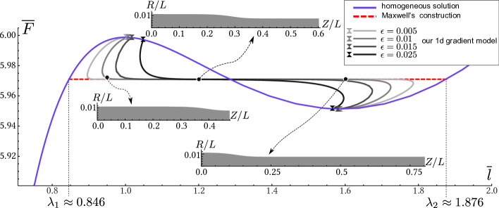
Figure 4: Bifurcation diagram predicted by the 1d gradient model in the $(\overline{l},\overline{F})$-plane for $\overline{\Gamma}=6$, where $\overline{l}=Z(L)/L$ is the average stretch ratio and $\overline{F}=F/(\pi G\rho^{2})$ is the scaled force. We consider symmetric modes with $\lambda^{\prime}(S=L/2)=0$. The gray curves were obtained by solving the 1d model using a continuation method for different aspect-ratios $\epsilon\in\{0.005,0.01,0.015,0.025\}$ (from light gray to black shades). The bifurcation condition (30) is represented by the hourglass symbols. The curve corresponding to homogeneous solutions, i.e., to a constant function $\lambda$, is drawn in blue; Maxwell’s construction is represented by the dotted red line. Insets: current configuration for $\epsilon=0.01$ at $\overline{l}=\{0.95,1.2,1.6\}$ (only the intersection of the half-plane $\Theta=0$ and of the half-cylinder $S\leq L/2$ is shown: the $Z/L$-axis is the axis of symmetry while the endpoint on the right is the center of the symmetric neck).

When following the bifurcation curves starting from the bifurcation point, the simulations capture a zone of localized axial stretch that grows progressively in amplitude while the axial force decreases (initiation); these solutions are unstable by standard symmetry exchange arguments, until the fold point where the axial forces starts to increase again. Further down the curve, the axial force converges to a Plateau value, independent on the value of $\epsilon$. The applied stretch can then be increased at a constant axial force, while the interface sweeps the length of the cylinder (propagation). Deformed shapes of the cylinder illustrating this evolution are drawn in Figure 4 for $\epsilon=0.01$.

The propagative behavior has been documented in other localized instabilities such as elastic necking or the bulging of elastic membranes (G’Sell et al., 1983; Kyriakides and Chang, 1991) and it can be interpreted as a phase transformation process (Chater and Hutchinson, 1984; Xuan and Biggins, 2017; Lestringant and Audoly, 2018). In this view, equilibrium solutions made of phases of constant strain are connected by sharp interfaces; the coexistence of these solutions is predicted by the 1d energy at order $\epsilon^{0}$, see equation (14). Consider two of such homogeneous phases in equilibrium, with axial stretch $\lambda_{1}$ and $\lambda_{2}$, and occupying fractions $f$ and $1-f$ of the initial domain (as measured by their extent in the Lagrangian domain $0\leq S\leq L/2$), respectively: the condition that the energy is stationary with respect to $\lambda_{1}$, $\lambda_{2}$ and $f$ writes

$$\begin{split}&\frac{\partial W_{\text{hom}}(\lambda)}{\partial\lambda}-F=0\quad\text{for}\quad\lambda=\lambda_{1}\quad\text{and}\quad\lambda=\lambda_{2},\\ &W_{\text{hom}}(\lambda_{1})-F\lambda_{1}=W_{\text{hom}}(\lambda_{2})-F\lambda_{2}.\end{split}$$ (31)

This system of equations can be solved for $\lambda_{1}$, $\lambda_{2}$ and $F$, which yields Maxwell’s plateau where two phases can be in equilibrium in an infinite domain (Maxwell, 1875; Xuan and Biggins, 2017). The plateau is shown by the dotted red line in the diagram in Figure 4: it provides an accurate prediction of the axial force observed during the propagation phase, when interfaces are well localized.

The strain gradient model goes one step beyond Maxwell’s construction by allowing the spatial distribution of the two phases, the width and the detailed shape of the interface to be determined. In Figure 5, we compare the deformed interface predicted by the 1d gradient model (continuous blue line) with that predicted by finite-element simulations of the full (3d-axisymmetric hyper-elastic) model (3) available from Xuan and Biggins (2017) (blue dots). We plot the scaled stretch ratio $\tilde{\lambda}(S)=\frac{2}{\lambda_{2}-\lambda_{1}}\left(\lambda(S)-\frac{\lambda_{1}+\lambda_{2}}{2}\right)$, where $\lambda_{1}$ and $\lambda_{2}$ are the transformation stretch ratios as determined by Maxwell’s construction (31), as a function of the scaled axial coordinate $\tilde{S}=\frac{S-S_{\mathrm{ct}}}{\rho}\sqrt{\overline{\Gamma}-\overline{\Gamma}_{\text{c}}}$; here $S_{\mathrm{ct}}$ is the Lagrangian coordinate at the center of the neck. In these scaled variables, the prediction of Xuan and Biggins’ weakly non-linear analysis (Xuan and Biggins, 2017) writes, see equation (14) in their paper,

$$\tilde{\lambda}(\tilde{S})=-\tanh\frac{2^{3/4}\tilde{S}}{\sqrt{17}}\qquad\qquad\textrm{(for $|\overline{\Gamma}-\overline{\Gamma}_{\mathrm{c}}|\ll 1$),}$$ (32)

and it is shown by the dashed brown line in Figure 5.

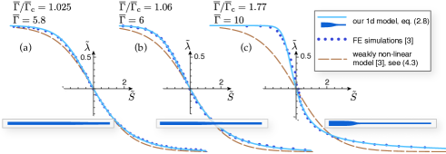
Figure 5: Solution for the interface in the propagation regime for different values of the rescaled surface tension $\overline{\Gamma}\in\{5.8,6,10\}$: solutions of the 1d gradient model with $\epsilon=0.01$ and an average stretch ratio $\overline{l}=1.2$ (light blue lines), finite element calculations in axisymmetric geometry from Xuan and Biggins (2017) (dark blue dots), and weakly non-linear gradient model from Xuan & Biggins (dashed brown curve). The actual shape of the bar predicted by the 1d gradient model is shown in the overlays in dark blue.

This weakly non-linear analysis captures the shape of the interface close to bifurcation, see Figure 5a. However, the agreement deteriorates in the post-bifurcation regime, the prediction on the scaled stretch $\tilde{\lambda}$ being underestimated by $\sim 10\%$ locally when $\overline{\Gamma}$ is 6% over the bifurcation threshold $\overline{\Gamma}_{\mathrm{c}}$, see Figure 5(b). By contrast, the 1d strain gradient model derived here remains highly accurate over a significantly larger range of values of $\overline{\Gamma}$, see Figure 5(c) in particular.

4.2 Varying elasto-capillary properties, keeping endpoints fixed

In the experiments of Mora et al. (2010), the amplitude of necking in cylinders having fixed endpoints has been measured in gels having different shear moduli $G$. In these experiments, the surface tension is $\Gamma=36.5\,10^{{-3}}\,\mathrm{N}\,\mathrm{m}^{-1}$ and the initial radius is $\rho=0.24\,\mathrm{mm}$, hence a scaled surface tension $\overline{\Gamma}=\Gamma/(\rho\,G)=(152\;\mathrm{Pa})/G$. With the aim to interpret these experiments, Taffetani and Ciarletta carried out non-linear finite element simulations of incompressible neo-Hookean cylinders subjected to surface tension (Taffetani and Ciarletta, 2015a), and investigated the post-buckled equilibria of the mode with $n$ wavelengths, i.e., having wavelength $\tilde{L}/n$, where $\tilde{L}=20\;\mathrm{mm}$ is the actual length of the cylinder used in the experiments. A comparison with the predictions of our 1d model is proposed in Figure 6. The 1d model was simulated by the same method as earlier in Figure 4, except that the parameter $\overline{\Gamma}$ was varied, and the force $\overline{F}$ was treated as an unknown set by the condition $\int_{0}^{L/2}\lambda(S)\,\mathrm{d}S=L/2$. In addition, the 1d model was solved numerically in a domain $0\leq S\leq L/2$ representing just a half wave of the buckling mode, i.e., a fraction $1/(2n)$ of the length $\tilde{L}$ of the cylinder in the experiments: $L=\tilde{L}/n$. With this choice, the buckling modes represented in the insets from Figures 4 and 6 match. Accordingly, we used in the 1d model an aspect-ratio $\epsilon=\rho/L=n\,\rho/\tilde{L}=0.012\,n$, where $\rho/\tilde{L}=0.012$ is the aspect-ratio in the experiments.

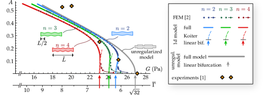
Figure 6: Necking in a cylinder having fixed endpoints: comparison of the predictions of the 1d model to the experiments of Mora et al. (2010) and to the finite-element simulations of Taffetani and Ciarletta (2015a). In all simulations, an incompressible neo-Hookean model is used: based on the experimental parameters from Mora et al. (2010), the shear modulus $G$ is connected to the scaled surface tension $\overline{\Gamma}$ by $G=152\;\mathrm{Pa}/\overline{\Gamma}$ (double horizontal axis). The amplitude $A$ of the modes comprising $n=2$, $3$, or $4$ full wavelengths are plotted (blue, green and red curves and data-points, respectively). The amplitude $A$ is defined as the maximum minus the minimum radius, divided by twice the initial radius. The gray curve is the prediction of the unregularized model. The agreement between the predictions of the 1d model (thick bright curves) and the finite-element simulations (dark dots) is excellent far from the bifurcation threshold; close to threshold, the finite-element simulations are affected by numerical imperfections (dark dots connected by thin dark curves). The buckling threshold (arrows) and the weakly non-linear prediction obtained by the Koiter method (dashed parabolas) derived from the 1d model agree well with its non-linear solutions; the instability is found to be sub-critical.

Far from the bifurcation threshold, the agreement in Figure 6 between the 1d model (bright thick curves) and the finite-element simulations (dots) is excellent; this confirms the accuracy of the 1d model in the deeply post-bifurcated regime, as seen already in Figure 5. Close to the bifurcation threshold, the agreement is significantly poorer but this is because the finite-element solution is affected by the imperfections that were introduced numerically to trigger buckling, as is evident from the ‘heels’ near the horizontal axis (dark thin curves connecting the dots); no such imperfections need to be introduced in the continuation method used to solve the 1d model. In fact, since the 1d model has been derived based on the assumption that the strain gradient $\lambda^{\prime}(S)$ is small, it is even more accurate close to threshold than far from threshold, even though the comparison to the finite element solution is not meaningful close to threshold.

We have carried out a weakly non-linear analysis of the 1d model to relate the dimensionless surface tension $\overline{\Gamma}$ to the buckling amplitude $A$ of the bifurcation mode $\lambda(S)=1-2\,A\,\cos(2\,\pi\,S/L)+\mathcal{O}(A^{2})=1-2\,A\,\cos(2\,n\,\pi\,S/\tilde{L})+\mathcal{O}(A^{2})$ close to threshold (the coeffient $-2\,A$ here warrants consistency with the amplitude $A$ defined in the legend in terms of the local radius $\rho\,\mu(S)=\rho\,\lambda^{-1/2}(S)$ reconstructed by the incompressibility condition). The weakly non-linear expansion is relatively straightforward to derive, and very similar to that presented in Lestringant and Audoly (2018) for the case of axisymmetric membranes; the details are not given here. The result is

$$\overline{\Gamma}=\overline{\Gamma}_{\mathrm{c}}(n)+\frac{\overline{\Gamma}^{\prime\prime}_{\mathrm{K}}(n)}{2}\,A^{2}+\mathcal{O}(A^{4}),$$ (33a)

where the critical parameter $$\overline{\Gamma}_{\mathrm{c}}(n) W_{\mathrm{hom}}^{\prime\prime}(\lambda)=-\frac{4\,\pi^{2}}{\tilde{L}^{2}/n^{2}}\,B_{\lambda} \lambda=1 \overline{\Gamma}^{\prime\prime}_{\mathrm{K}}(n)$$ is such that at , as earlier in equation (30), and the coefficient given by the Koiter method writes

$$\overline{\Gamma}^{\prime\prime}_{\mathrm{K}}(n)=\frac{3(4(-8+\overline{\Gamma})^{2}-4\overline{k}_{n}^{2}(24-83\overline{\Gamma}+13\overline{\Gamma}^{2})+\overline{k}_{n}^{4}(9-28\overline{\Gamma}+60\overline{\Gamma}^{2}))}{16\overline{k}_{n}^{2}(-1+\overline{k}_{n}^{2})\overline{\Gamma}},\quad\overline{k}_{n}=2\pi\,\frac{n\,\rho}{\tilde{L}}$$ (33b)

The predictions of this weakly non-linear analysis are shown by the dashed curves in the figure, and agree very well with the non-linear simulations of the 1d model. For the set of parameters used here, we find $\overline{\Gamma}^{\prime\prime}_{\mathrm{K}}(n)<0$, implying that the bifurcation is a sub-critical (discontinuous) pitchfork bifurcation: along the bifurcated curves in figure 6 (light thicker curves) and for an increasing amplitude $A$, the parameter $\overline{\Gamma}$ initially decreases close to bifurcation but the branch goes through an inflexion point soon after and $\overline{\Gamma}$ increases with $A$.

A weakly non-linear analysis of an incompressible neo-Hookean cylinder with surface tension in axisymmetric geometry was carried out in Taffetani and Ciarletta (2015a). For the same set of parameters as those used in Figure 6, the authors concluded that the bifurcation is super-critical (continuous), which is at odds with our own conclusion. Our previous analysis of bulging in axisymmetric membranes (Lestringant and Audoly, 2018) shows that the 1d model captures amplitude equations such as (33a) correctly at the dominant order: the assumption $|\lambda^{\prime}|\ll 1/L$ is well satisfied close to threshold. The weakly non-linear analyses based on the 1d model in equation (33) and that reported in Taffetani and Ciarletta (2015a) should give exactly the same result. We are confident that our result (33) is correct as (i) it accurately matches the non-linear solutions close to threshold—such a verification could not be made in Taffetani and Ciarletta (2015a) due to the presence of the numerical imperfections, see the ‘heels’ in figure 6—, (ii) the weakly non-linear expansion based on the 1d model is considerably simpler than that based on the full model, and therefore less prone to errors, and (iii) a close examination of the finite-element results reveals a jump in the amplitude (a gap in the blue dots around $G=25\;\mathrm{Pa}$ is visible in figure 6), which suggests that a discontinuity, not entirely suppressed by the smoothing effect of the numerical imperfections, is indeed present.

Far from threshold, the bifurcation branches for $2\leq n\leq 4$ are all well approximated by the curve shown in gray. The gray curve has been obtained from the unregularized model as follows: for any value of $\overline{\Gamma}$, the transformation stretches $\lambda_{1}$ and $\lambda_{2}$ have been calculated using Maxwell’s construction, see equation (31), and the necking amplitude has been defined based on the two phases in equilibrium as $A=(\lambda_{2}^{{-1/2}}-\lambda_{1}^{-1/2})/2$. In this unregularized model, the interfaces are treated as discontinuities and the detailed distribution of the coexisting phases along the length of the cylinder remains undefined, but this is of no importance here. The unregularized model gives similar predictions as the 1d gradient model when the amplitude is larger than $A\stackrel{{\scriptstyle>}}{{\sim}}0.3$: this is because the buckling mode, which is initially evenly distributed along the entire length of the cylinder, localizes quickly in the post-bifurcation regime, thereby mimicking the predictions of the unregularized model. Overall, the unregularized model, despite being quite simple, captures the general trend in the experimental data-points fairly well.

In the bifurcation diagram in Figure 6, the Koiter expansion appears to have a very limited range of validity. This is caused by the quick localization of the bifurcation mode in the post-bifurcation regime, a phenomenon that is not captured by the Koiter expansion (a similar issue arises in spherical shell buckling (Audoly and Hutchinson, 2020) in an even more severe form). This fast localization phenomenon is not captured by the weakly non-linear approaches that have been used in earlier work on elasto-capillary necking. By contrast, our 1d model accurately captures localization, by retaining the relevant nonlinearity in both the unregularized potential $W_{\mathrm{hom}}(\lambda)$ and in the second gradient modulus $B_{\lambda}$.

5 Conclusion

We derived a 1d strain gradient model for the elasto-capillary necking of soft hyper-elastic cylinders. A generic, transversely symmetric elastic constitutive law has been considered, which includes isotropic materials as a particular case; the case of an incompressible neo-Hookean material has been considered as an application. The model has been derived starting from a kinematic ansatz for the sake of brevity, but the particular form of the displacement used as a starting point can be justified from a systematic reduction method (Lestringant and Audoly, 2020). It can also be checked that the solution thus constructed satisfies the equations of equilibrium at the dominant orders. The resulting model is asymptotically correct in the limit where the ratio $\epsilon$ of the radius $\rho$ to the typical scale of variation of the longitudinal stretch $\lambda(S)$ is small, $\epsilon\ll 1$.

Our model consists of a non-convex strain energy density depending on the axial stretch ratio $\lambda(S)$ at leading order $\epsilon^{0}$, regularized by a term depending quadratically on the strain gradient $\lambda^{\prime}(S)$ and non-linearly on $\lambda(S)$. This regularizing term is formally of order $\epsilon^{2}$. Expressions for all the coefficients entering the 1d strain energy functional have been derived in terms of the cylinder’s radius and of the hyper-elastic constitutive behavior. It is a distinctive and crucial feature of our 1d model that the non-linear dependence of the energy on $\lambda(S)$ is retained. This warrants accurate predictions in a broad range of parameters, as shown by the comparison with finite element simulations of the full 3d finite-strain elasticity problem.

Besides being significantly easier to solve numerically, the 1d model is easily amenable to linear and weakly nonlinear bifurcation analyses. It also reveals the deep analogy with other propagative instabilities and with phase transitions: the 1d model which we derived is akin to the diffuse-interface model introduced by van der Waals for the analysis of the liquid-vapor phase transition (van der Waals, 1894). Despite its simplicity, it is remarkably accurate, even beyond the onset of localization where it is mathematically justified. This unexpected accuracy is manifest on the third plot in Figure 5, when the bifurcation parameter is as large as $\overline{\Gamma}/\overline{\Gamma}_{\mathrm{c}}=10/5.7=1.77$, as well as in Figure 6. A similar, unexpectedly broad domain of validity has been reported with the 1d strain gradient model derived for the analysis of the bulging of axisymmetric membranes (Lestringant and Audoly, 2018). There is probably a common explanation for these nice surprises but we could not identify it. We hope that this intriguing fact will be investigated further.

Ethics statement. This work did not involve any ethical issue.
Data accessibility statement. This work does not have any experimental data.
Competing interests statement. We have no competing interests.
Authors’ contributions. Both authors have equally contributed to all aspects of the work.
Funding. There has been no dedicated funding for this work.
Acknowledgments. We would like to thank Serge Mora for sharing pictures of his experiments.

Appendix A Elimination of the boundary terms

The dimension reduction produces boundary terms $[C_{\lambda}\,\lambda^{\prime}]_{0}^{L}$ in the energy functional (28a). These boundary term make the variational problem of equilibrium ill-posed. In this appendix, we fix this issue by introducing an alternate definition of the centroid $z(S)$ of the cross-sections. When expressed in terms of the new centroid, the energy functional has no boundary terms, and the equations of equilibrium can be obtained variationally. This change of unknown amounts to discard the boundary term $\mathrm{C}_{\lambda}$, and to add another contribution to the coefficient $\mathrm{B}_{\lambda}$.

Moving the boundary term in (28a) under the integration sign yields

$$\Phi_{\text{1d}}[\lambda]=\int_{0}^{L}\left(W_{\text{hom}}(\lambda(S))+\frac{1}{2}\left(\mathrm{B}_{\lambda(S)}+2\frac{\mathrm{d}\mathrm{C}_{\lambda}}{\mathrm{d}\lambda}(\lambda(S))\right)\lambda^{\prime 2}(S)+\mathrm{C}_{\lambda(S)}\lambda^{\prime\prime}(S)\right)\mathrm{d}S+\mathcal{O}(L\varepsilon^{3}).$$

With a view of eliminating the second derivative of $\lambda$ in this energy functional, we change the definition of the centroid to

$$z_{\star}(S)=z(S)+f(\lambda(S))\lambda^{\prime}(S),$$ (A.34)

where the function $f(\lambda)$ will be specified later. With the aim to motivate this change of variable, we observe that it is akin to switching from the uniform averaging in (4), to a weighted average with weight $g(R)$ in the cross-section, i.e., $z_{\star}=\int_{0}^{L}g(T)Z(S,T)2\pi T\mathrm{d}T$. Indeed, the latter yields, in view of the curvature effect, $z_{\star}\sim z+\mathcal{A}(S)\int_{0}^{L}g(T)t(T)2\pi T\mathrm{d}T\sim z+\lambda^{\prime}(S)\int_{0}^{L}g(T)t(T)2\pi T\mathrm{d}T$, which is indeed of the same form as (A.34).

With the new centroid definition (A.34), the apparent stretch becomes

$$\lambda_{\star}(S)=\frac{\mathrm{d}z_{\star}}{\mathrm{d}S}=\frac{\mathrm{d}z}{\mathrm{d}S}+\frac{\mathrm{d}f}{\mathrm{d}\lambda}\lambda^{\prime 2}+f\lambda^{\prime\prime}=\lambda(S)+\frac{\mathrm{d}f}{\mathrm{d}\lambda}(\lambda(S))\lambda^{\prime 2}(S)+f(\lambda(S))\lambda^{\prime\prime}(S).$$

As both terms $\frac{\mathrm{d}f}{\mathrm{d}\lambda}\lambda^{\prime 2}$ and $f\lambda^{\prime\prime}$ are of order $\varepsilon^{2}$, this relation can be inverted as $\lambda(S)=\lambda_{\star}(S)-\left(\frac{\mathrm{d}f}{\mathrm{d}\lambda}(\lambda_{\star}(S))\lambda_{\star}^{\prime 2}(S)+f(\lambda_{\star}(S))\lambda_{\star}^{\prime\prime}(S)\right)+\mathcal{O}(\varepsilon^{4})$. In terms of $\lambda_{\star}$, the energy functional writes

$$\begin{array}[]{lll}\Phi_{\text{1d}}[\lambda_{\star}]&=&\int_{0}^{L}\left[W_{\text{hom}}\left(\lambda_{\star}(S)-\frac{\mathrm{d}f}{\mathrm{d}\lambda}(\lambda_{\star}(S))\lambda_{\star}^{\prime 2}(S)-f(\lambda_{\star}(S))\lambda_{\star}^{\prime\prime}(S)\right)\cdots\right.\\ &&\hskip 40.00006pt\left.+\frac{1}{2}\left(\mathrm{B}_{\lambda_{\star}(S)}+2\frac{\mathrm{d}\mathrm{C}_{\lambda}}{\mathrm{d}\lambda}(\lambda_{\star}(S))\right)\lambda^{\prime 2}(S)+\mathrm{C}_{\lambda_{\star}(S)}\lambda_{\star}^{\prime\prime}(S)\mathrm{d}S\right]+\mathcal{O}(L\varepsilon^{3}),\\ &=&\int_{0}^{L}\left[W_{\text{hom}}(\lambda_{\star}(S))+\frac{1}{2}\left(\mathrm{B}_{\lambda_{\star}(S)}+2\frac{\mathrm{d}\mathrm{C}_{\lambda}}{\mathrm{d}\lambda}(\lambda_{\star}(S))-2\frac{\mathrm{d}W_{\text{hom}}}{\mathrm{d}\lambda}(\lambda_{\star}(S))\frac{\mathrm{d}f}{\mathrm{d}\lambda}(\lambda_{\star}(S))\right)\lambda_{\star}^{\prime 2}(S)\right.\cdots\\ &&\hskip 40.00006pt\left.+\left(\mathrm{C}_{\lambda_{\star}(S)}-\frac{\mathrm{d}W_{\text{hom}}}{\mathrm{d}\lambda}(\lambda_{\star}(S))f(\lambda_{\star}(S))\right)\lambda_{\star}^{\prime\prime}(S)\right]\mathrm{d}S+\mathcal{O}(L\varepsilon^{3}).\end{array}$$

With the particular definition

$$f(\lambda)=\frac{\mathrm{C}_{\lambda}}{\frac{\mathrm{d}W_{\text{hom}}}{\mathrm{d}\lambda}(\lambda)},$$ (A.35)

the term proportional to $\lambda_{\star}^{\prime\prime}(S)$ cancels in the new energy functional. This corresponds to a re-definition of the centroid (A.34) and of the stretch measure as

$$z_{\star}=z+\frac{\mathrm{C}_{\lambda}}{\frac{\mathrm{d}W_{\text{hom}}}{\mathrm{d}\lambda}}\lambda^{\prime},\qquad\lambda_{\star}=\lambda+\frac{\mathrm{d}}{\mathrm{d}\lambda}\left(\frac{\mathrm{C}_{\lambda}}{\frac{\mathrm{d}W_{\text{hom}}}{\mathrm{d}\lambda}}\right)\lambda^{\prime 2}+\frac{\mathrm{C}_{\lambda}}{\frac{\mathrm{d}W_{\text{hom}}}{\mathrm{d}\lambda}}\lambda^{\prime\prime}\textrm{.}$$ (A.36)

Note that both $\lambda$ and $\lambda_{\star}$ are of order 1, while the correction is small, of order $\epsilon^{2}$.

Inserting the expression of $f$ in the expression of the energy above, we find

$$\Phi_{\text{1d}}[\lambda_{\star}]=\int_{0}^{L}\left(W_{\text{hom}}(\lambda_{\star}(S))+\frac{1}{2}\mathrm{D}_{\lambda_{\star}(S)}\lambda_{\star}^{\prime 2}(S)\right)\mathrm{d}S+\mathcal{O}(L\,\varepsilon^{3}),$$ (A.37a)

where

$$\mathrm{D}_{\lambda_{\star}}=\mathrm{B}_{\lambda_{\star}}+2\mathrm{C}_{\lambda_{\star}}\frac{\frac{\mathrm{d}^{2}W_{\text{hom}}}{\mathrm{d}\lambda^{2}}(\lambda_{\star})}{\frac{\mathrm{d}W_{\text{hom}}}{\mathrm{d}\lambda}(\lambda_{\star})}.$$ (A.37b)

A comparison of the original energy (28a) and the one just derived shows that the boundary terms in the energy can be discarded provided the elastic modulus $B_{\lambda}$ is replaced with $D_{\lambda}$.

Appendix B 1d model for an incompressible neo-Hookean material

The strain energy of a quasi-incompressible neo-Hookean material with a shear modulus $G$, subjected to an equi-biaxial strain of axial stretch $\lambda$ and radial strain $\mu$, can be written as

$$w(\lambda,\mu)=\frac{G}{2}\left(\lambda^{2}+2\,\mu^{2}\right)+\frac{1}{2\,\eta}\,\left(\lambda\,\mu^{2}-1\right)^{2},$$

where $\eta\ll 1$ is a penalization parameter enforcing inextensibility. There are different ways to this energy that are equivalent in the limit $\eta\to 0$, and we picked a simple one. The transverse equilibrium (7) yields

$$2\,G\,\mu+\frac{1}{\eta}\,\left(\lambda\,\mu^{2}-1\right)\,2\,\mu\,\lambda+\frac{2\,\Gamma}{\rho}\,\lambda=0.$$ (B.38)

From (6), the axial Piola-Kirchhoff stress is $\Sigma^{\parallel}=\frac{1}{\lambda}\,\frac{\partial w}{\partial\lambda}=G+\frac{1}{\eta}\,\left(\lambda\,\mu^{2}-1\right)\,\frac{\mu^{2}}{\lambda}$. Inserting the hydrostatic pressure $\frac{1}{\eta}\,\left(\lambda\,\mu^{2}-1\right)$ found from (B.38), we have $\Sigma^{\parallel}=\frac{1}{\lambda}\,\frac{\partial w}{\partial\lambda}=G\,\left(1-\frac{\mu}{\lambda}\,\overline{\Gamma}-\,\frac{\mu^{2}}{\lambda^{2}}\right)$. In the incompressible limit, $\eta\rightarrow 0$ and $\mu_{\lambda}=\lambda^{-1/2}$, so that

$$\Sigma^{\parallel}_{\text{hom}}(\lambda)=G\,\left(1-\frac{\overline{\Gamma}}{\lambda^{3/2}}-\,\frac{1}{\lambda^{3}}\right).$$

The tangent shear modulus $K_{\mathrm{hom}}^{{STST}}(\lambda)$ can be found by considering a shear perturbation $\hat{\mathbf{E}}=\hat{E}_{ST}\,(\mathbf{d}_{S}\otimes\mathbf{d}_{T}+\mathbf{d}_{T}\otimes\mathbf{d}_{S})$ to the equi-biaxial strain $\mathbf{E}_{\mathrm{hom}}(\lambda,\lambda^{{-1/2}})$, as in (17a), by expanding the strain energy, and by identifying the result with with (17b). This yields

$$K_{\text{hom}}^{STST}(\lambda)=G\,\left(\lambda^{-2}+\overline{\Gamma}\,\lambda^{{-1/2}}\right).$$ (B.39)

The potential of the unregularized model reads from (8b)

$$W_{\text{hom}}(\lambda)=\frac{\pi\,\rho^{2}\,G}{2}\,\left(\lambda^{2}+\frac{2}{\lambda}+4\,\overline{\Gamma}\,\lambda^{1/2}\right),$$ (B.40)

as announced earlier in equation (15), and in equation 2 in Xuan and Biggins (2017).

The gradient of transverse stretch defined in (8d) reads $\nabla\mu_{\lambda}=\frac{\mathrm{d}\mu_{\lambda}}{\mathrm{d}\lambda}=\frac{\mathrm{d}\lambda^{-1/2}}{\mathrm{d}\lambda}=-\frac{1}{2\,\lambda^{3/2}}$, and we find the gradient moduli in the energy (28a) from (28b) as

$$\frac{1}{2}\,B_{\lambda}=\frac{\pi\,\rho^{4}\,G}{16\,\lambda^{6}}\,\left(\lambda^{3}+4\,\overline{\Gamma}\,\lambda^{3/2}-1\right),\qquad\qquad C_{\lambda}=\frac{\pi\,\rho^{4}\,G}{4\,\lambda^{7/2}}\,\overline{\Gamma}.$$ (B.41)

The elimination of boundary terms using the method in appendix A is carried out by inserting (B.40) and (B.41) into (A.37b), which yields

$$\frac{1}{2}\,D_{\lambda}=\frac{\pi\,\rho^{4}\,G}{16\,\lambda^{6}}\,\frac{(\lambda^{3}-1)^{2}+3\,\overline{\Gamma}\,\lambda^{3/2}\,\left(3\,\lambda^{3}+1\right)+2\,\overline{\Gamma}^{2}\,\lambda^{3}}{\lambda^{3}+\overline{\Gamma}\,\lambda^{3/2}-1}.$$ (B.42)

The relative change in second-gradient modulus $\left|\frac{D_{\lambda}-B_{\lambda}}{B_{\lambda}}\right|$ is typically less that 10% for $\overline{\Gamma}\leq 10$ and $1\leq\lambda\leq 2$.

References

- Audoly and Hutchinson (2016) B. Audoly and J. W. Hutchinson. Analysis of necking based on a one-dimensional model. Journal of the Mechanics and Physics of Solids, 97:68–91, 2016.
- Audoly and Hutchinson (2020) B. Audoly and J. W. Hutchinson. Localization in spherical shell buckling. Journal of the Mechanics and Physics of Solids, 136:103720, 2020.
- Brunetti et al. (2020) M. Brunetti, A. Favata, and S. Vidoli. From Föppl–von Kármán shells to enhanced one-dimensional rods: localization phenomena and multistability. arXiv:2003.09425v1, 2020.
- Carr et al. (1984) J. Carr, M. E. Gurtin, and M. Slemrod. Structured phase transitions on a finite interval. Archive for Rational Mechanics and Analysis, 86:317–351, 1984.
- Chater and Hutchinson (1984) E. Chater and J. W. Hutchinson. On the propagation of bulges and buckles. Journal of Applied Mechanics, 51:269–277, 1984.
- Doedel et al. (2007) E. J. Doedel, A. R. Champneys, T. F. Fairgrieve, Y. A. Kuznetsov, B. Sandstede, and X. J. Wang. AUTO-07p: continuation and bifurcation software for ordinary differential equations. See http://indy.cs.concordia.ca/auto/, 2007.
- Ericksen (1975) J. L. Ericksen. Equilibium of bars. Journal of Elasticity, 5:191, 1975.
- G’Sell et al. (1983) C. G’Sell, N. A. Aly-Helal, and J. J. Jonas. Effect of stress triaxiality on neck propagation during the tensile stretching of solid polymers. Journal of Materials Science, 18:1731–1742, 1983.
- Kyriakides and Chang (1991) S. Kyriakides and Yu-Chung Chang. The initiation and propagation of a localized instability in an inflated elastic tube. International Journal of Solids and Structures, 27(9):1085–1111, 1991.
- Lestringant and Audoly (2018) C. Lestringant and B. Audoly. A diffuse interface model for the analysis of propagating bulges in cylindrical balloons. Proceedings of the Royal Society A: Mathematical, Physical and Engineering Sciences, 474:20180333, 2018.
- Lestringant and Audoly (2020) Claire Lestringant and Basile Audoly. Asymptotically exact strain-gradient models for nonlinear slender elastic structures: A systematic derivation method. Journal of the Mechanics and Physics of Solids, 136:103730, 2020.
- Martin et al. (2020) M Martin, Stéphane Bourgeois, B Cochelin, and F Guinot. Planar folding of shallow tape springs: The rod model with flexible cross-section revisited as a regularized ericksen bar model. International Journal of Solids and Structures, 188:189–209, 2020.
- Maxwell (1875) J. C. Maxwell. On the dynamical evidence of the molecular constitution of bodies. Nature, 11:357, 1875.
- Mora et al. (2010) Serge Mora, Ty Phou, Jean-Marc Fromental, Len M Pismen, and Yves Pomeau. Capillarity driven instability of a soft solid. Physical review letters, 105(21):214301, 2010.
- Taffetani and Ciarletta (2015a) Matteo Taffetani and Pasquale Ciarletta. Beading instability in soft cylindrical gels with capillary energy: weakly non-linear analysis and numerical simulations. Journal of the Mechanics and Physics of Solids, 81:91–120, 2015a.
- Taffetani and Ciarletta (2015b) Matteo Taffetani and Pasquale Ciarletta. Elastocapillarity can control the formation and the morphology of beads-on-string structures in solid fibers. Physical Review E, 91(3):032413, 2015b.
- van der Waals (1894) J. D. van der Waals. Thermodynamische Theorie der Kapillarität unter Voraussetzung stetiger Dichteänderung. Z. Phys. Chem., 13:657–725, 1894.
- Xuan and Biggins (2017) Chen Xuan and John Biggins. Plateau-Rayleigh instability in solids is a simple phase separation. Physical Review E, 95(5):053106, 2017.