On the Bottleneck of Graph Neural Networks
and its Practical Implications

Abstract

Since the proposal of the graph neural network (GNN) by Gori et al. [2005] and Scarselli et al. [2008], one of the major problems in training GNNs was their struggle to propagate information between distant nodes in the graph. We propose a new explanation for this problem: GNNs are susceptible to a bottleneck when aggregating messages across a long path. This bottleneck causes the over-squashing of exponentially growing information into fixed-size vectors. As a result, GNNs fail to propagate messages originating from distant nodes and perform poorly when the prediction task depends on long-range interaction. In this paper, we highlight the inherent problem of over-squashing in GNNs: we demonstrate that the bottleneck hinders popular GNNs from fitting long-range signals in the training data; we further show that GNNs that absorb incoming edges equally, such as GCN and GIN, are more susceptible to over-squashing than GAT and GGNN; finally, we show that prior work, which extensively tuned GNN models of long-range problems, suffer from over-squashing, and that breaking the bottleneck improves their state-of-the-art results without any tuning or additional weights. Our code is available at https://github.com/tech-srl/bottleneck/ .

1 Introduction

Graph neural networks (GNNs) Gori et al. [2005], Scarselli et al. [2008], Micheli [2009] have seen sharply growing popularity over the last few years Duvenaud et al. [2015], Hamilton et al. [2017], Xu et al. [2019]. GNNs provide a general framework to model complex structural data containing elements (nodes) with relationships (edges) between them. A variety of real-world domains such as social networks, computer programs, chemical and biological systems can be naturally represented as graphs. Thus, many graph-structured domains are commonly modeled using GNNs.

A GNN layer can be viewed as a message-passing step Gilmer et al. [2017], where each node updates its state by aggregating messages flowing from its direct neighbors. GNN variants Li et al. [2016], Veličković et al. [2018], Kipf and Welling [2017] mostly differ in how each node aggregates the representations of its neighbors with its own representation. However, most problems also require the interaction between nodes that are not directly connected, and they achieve this by stacking multiple GNN layers. Different learning problems require different ranges of interaction between nodes in the graph to be solved. We call this required range of interaction between nodes – the problem radius.

In practice, GNNs were observed not to benefit from more than few layers. The accepted explanation for this phenomenon is over-smoothing: node representations become indistinguishable when the number of layers increases Wu et al. [2020]. Nonetheless, over-smoothing was mostly demonstrated in short-range tasks Li et al. [2018], Klicpera et al. [2018], Chen et al. [2020a], Oono and Suzuki [2020], Zhao and Akoglu [2020], Rong et al. [2020], Chen et al. [2020b] – tasks that have small problem radii, where a node’s correct prediction mostly depends on its local neighborhood. Such tasks include paper subject classification Sen et al. [2008] and product category classification Shchur et al. [2018]. Since the learning problems depend mostly on short-range information in these datasets, it makes sense why more layers than the problem radius might be extraneous. In contrast, in tasks that also depend on long-range information (and thus have larger problem radii), we hypothesize that the explanation for limited performance is over-squashing. We further discuss the differences between over-squashing and over-smoothing in Section 6.

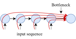
(a) The bottleneck of RNN seq2seq models

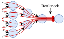
(b) The bottleneck of graph neural networks

Figure 1: The bottleneck that existed in RNN seq2seq models (before attention) is strictly more harmful in GNNs: information from a node’s exponentially-growing receptive field is compressed into a fixed-size vector. Black arrows are graph edges; red curved arrows illustrate information flow.

To allow a node to receive information from other nodes at a radius of $K$, the GNN needs to have at least $K$ layers, or otherwise, it will suffer from under-reaching – these distant nodes will simply not be aware of each other. Clearly, to avoid under-reaching, problems that depend on long-range interaction require as many GNN layers as the range of the interaction. However, as the number of layers increases, the number of nodes in each node’s receptive field grows exponentially. This causes over-squashing: information from the exponentially-growing receptive field is compressed into fixed-length node vectors. Consequently, the graph fails to propagate messages flowing from distant nodes, and learns only short-range signals from the training data.

In fact, the GNN bottleneck is analogous to the bottleneck of sequential RNN models. Traditional seq2seq models Sutskever et al. [2014], Cho et al. [2014a, b] suffered from a bottleneck at every decoder state – the model had to encapsulate the entire input sequence into a fixed-size vector. In RNNs, the receptive field of a node grows linearly with the number of recursive applications. However in GNNs, the bottleneck is asymptotically more harmful, because the receptive field of a node grows exponentially. This difference is illustrated in Figure 1.

This work does not aim to propose a new GNN variant. Rather, our main contribution is introducing the over-squashing phenomenon – a novel explanation for the major and well-known issue of training GNNs for long-range problems, and showing its harmful practical implications. We use a controlled problem to demonstrate how over-squashing prevents GNNs from fitting long-range patterns in the data, and to provide theoretical lower bounds for the required hidden size given the problem radius (Section 5). We show, analytically and empirically, that GCN Kipf and Welling [2017] and GIN Xu et al. [2019] are susceptible to over-squashing more than other types of GNNs such as GAT Veličković et al. [2018] and GGNN Li et al. [2016]. We further show that prior work that extensively tuned GNNs to real-world datasets suffer from over-squashing: breaking the bottleneck using a simple fully adjacent layer reduces the error rate by 42% in the QM9 dataset, by 12% in ENZYMES, by 4.8% in NCI1, and improves accuracy in VarMisuse, without any additional tuning.

2 Preliminaries

A directed graph $\mathcal{G}=\left(\mathcal{V},\mathcal{E}\right)$ contains nodes $\mathcal{V}$ and edges $\mathcal{E}$, where $\left(u,v\right)\in\mathcal{E}$ denotes an edge from a node $u$ to a node $v$. For brevity, in the following definitions we treat all edges as having the same type; in general, every edge can have a type and features Schlichtkrull et al. [2018].

Graph neural networks Graph neural networks operate by propagating neural messages between neighboring nodes. At every propagation step (a graph layer): the network computes each node’s sent message; every node aggregates its received messages; and each node updates its representation by combining the aggregated incoming messages with its own previous representation.

Formally, each node is associated with an initial representation $\mathbf{h}_{v}^{\left(0\right)}\in\mathcal{R}^{d_{0}}$. This representation is usually derived from the node’s label or its given features. Then, a GNN layer updates each node’s representation given its neighbors, yielding $\mathbf{h}_{v}^{\left(1\right)}\in\mathcal{R}^{d}$. In general, the $k$-th layer of a GNN is a parametric function $f_{k}$ that is applied to each node by considering its neighbors:

$$\mathbf{h}_{v}^{\left(k\right)}=f_{k}\left(\mathbf{h}_{v}^{\left(k-1\right)},\{\mathbf{h}_{u}^{\left(k-1\right)}\mid u\in\mathcal{N}_{v}\};\theta_{k}\right)$$ (1)

where $\mathcal{N}_{v}$ is the set of nodes that have edges to $v$: $\mathcal{N}_{v}=\{u\in\mathcal{V}\mid\left(u,v\right)\in\mathcal{E}\}$. The total number of layers $K$ is usually determined empirically as a hyperparameter.

The design of the function $f$ is what mostly distinguishes one type of GNN from the other. For example, graph convolutional networks (GCN) define $f$ as:

$$\mathbf{h}_{v}^{\left(k\right)}=\sigma\left(\sum\nolimits_{u\in\mathcal{N}_{v}\cup\{v\}}\frac{1}{c_{u,v}}W^{\left(k\right)}\mathbf{h}_{u}^{\left({k-1}\right)}\right)$$ (2)

where $\sigma$ is a nonlinearity such as $ReLU$, and $c_{u,v}$ is a normalization factor often set to $\sqrt{|\mathcal{N}_{v}|\cdot|\mathcal{N}_{u}}|$ or $|\mathcal{N}_{v}|$ Hamilton et al. [2017]. As another example, graph isomorphism networks (GIN) Xu et al. [2019] update a node’s representation using the following definition:

$$\mathbf{h}_{v}^{\left(k\right)}=MLP^{\left(k\right)}\left(\left(1+\epsilon^{\left(k\right)}\right)\mathbf{h}_{v}^{\left(k-1\right)}+\sum\nolimits_{u\in\mathcal{N}_{v}}\mathbf{h}_{u}^{\left({k-1}\right)}\right)$$ (3)

Usually, the last ($K$-th) layer’s output is used for prediction: in node-prediction, $\mathbf{h}_{v}^{\left(K\right)}$ is used to predict a label for $v$; in graph-prediction, a permutation-invariant “readout” function aggregates the nodes of the final layer using summation, averaging, or a weighted sum Li et al. [2016].

3 The GNN Bottleneck

Given a graph $\mathcal{G}=\left(\mathcal{V},\mathcal{E}\right)$ and a given node $v$, we denote the problem’s required range of interaction, the problem radius, by $r$. $r$ is generally unknown in advance, and usually approximated empirically by tuning the number of layers $K$. We denote the set of nodes in the receptive field of $v$ by $\mathcal{N}_{v}^{K}$, which is defined recursively as $\mathcal{N}_{v}^{1}:=\mathcal{N}_{v}$ and $\mathcal{N}_{v}^{K}:=\mathcal{N}_{v}^{K-1}\cup\{w\mid\left(w,u\right)\in\mathcal{E}\land u\in\mathcal{N}_{v}^{K-1}\}$.

When a prediction problem relies on long-range interaction between nodes, the GNN must have as many layers $K$ as the estimated range of these interactions, or otherwise, these distant nodes would not be able to interact. It is thus required that $K\geq r$. However, the number of nodes in each node’s receptive field grows exponentially with the number of layers: $\left\lvert\mathcal{N}_{v}^{K}\right\rvert=\mathcal{O}\left(\exp\left(K\right)\right)$ Chen et al. [2018]. As a result, an exponentially-growing amount of information is squashed into a fixed-length vector (the vector resulting from the $\sum$ in Equations 2 and 3), and crucial messages fail to reach their distant destinations. Instead, the model learns only short-ranged signals from the training data and consequently might generalize poorly at test time.

Figure 2: The NeighborsMatch: green nodes ( , , ) have blue neighbors ( ) and an alphabetical label. The goal is to predict the label (A, B, or C) of the green node that has the same number of blue neighbors as the target node ( ) in the same graph. In this example, the correct label is C, because the target node has two blue neighbors, like the node marked with C in the same graph.

Example Consider the NeighborsMatch problem of Figure 2. Green nodes ( , , ) have a varying number of blue neighbors ( ) and an alphabetical label. Each example in the dataset is a different graph that has a different mapping from numbers of neighbors to labels. The rest of the graph (marked as ) represents a general, unknown, graph structure. The goal is to predict a label for the target node, which is marked with a question mark ( ), according to its number of blue neighbors. The correct answer is C in this case, because the target node has two blue neighbors, like the node marked with C in the same graph. Every example in the dataset has a different mapping from numbers of neighbors to labels, and thus message propagation and matching between the target node and all the green nodes must be performed for every graph in the dataset.

Since the model must propagate information from all green nodes before predicting the label, a bottleneck at the target node is inevitable. This bottleneck causes over-squashing, which can prevent the model from fitting the training data perfectly. We demonstrate the bottleneck empirically in this problem in Section 4; in Section 5, we provide theoretical lower bounds for the GNN’s hidden size. Obviously, adding direct edges between the target node and the green nodes, or making the existing edges bidirectional, could ease information flow for this specific problem. However, in real-life domains (e.g., molecules), we do not know the optimal message propagation structure a priori, and must use the given relations (such as bonds between atoms) as the graph’s edges.

Although this is a contrived problem, it resembles real-world problems that are often modeled as graphs. For example, a computer program in a language such as Python may declare multiple variables (i.e., the green nodes in Figure 2) along with their types and values (their numbers of blue neighbors in Figure 2); later in the program, predicting which variable should be used in a specific location (predict the alphabetical label in Figure 2) must use one of the variables that are available in scope based on the required type and the required value at that point. We experiment with this VarMisuse problem in Section 4.4.

Short- vs. long-range problems Much of prior GNN work has focused on problems that were local in nature, with small problem radii, where the underlying inductive bias was that a node’s most relevant context is its local neighborhood, and long-range interaction was not necessarily needed. With the growing popularity of GNNs, their adoption expanded to domains that required longer-range information propagation as well, without addressing the inherent bottleneck. In this paper, we focus on problems that require long-range information. That is, a correct prediction requires considering the local environment of a node and interactions beyond the close neighborhood. For example, a chemical property of a molecule Ramakrishnan et al. [2014], Gilmer et al. [2017] can depend on the combination of atoms that reside in the molecule’s opposite sides. Problems of this kind require long-range interaction, and thus, a large number of GNN layers. Since the receptive field of each node grows exponentially with the number of layers, the more layers – over-squashing is more harmful.

In problems that are local in nature (small $r$) – the bottleneck is less troublesome, because a GNN can perform well with only few layers (e.g., $K$$=$2 layers in Kipf and Welling [2017]), and the receptive field of a node can be exponentially smaller. Domains such as citation networks Sen et al. [2008], social networks Leskovec and Mcauley [2012], and product recommendations Shchur et al. [2018] usually raise short-range problems and are thus not the focus of this paper. So, how long is long-range? We discuss and analyze this question in Section 5.

4 Evaluation

First, we wish to empirically show that the GNN bottleneck exists, and find the smallest values of $r$ that raise over-squashing. We generated a synthetic benchmark that is theoretically solvable; however, in practice, all GNNs fail to reach 100% training accuracy because of the bottleneck (Section 4.1). Second, we examine whether the bottleneck exists in prior work, which addressed real-world problems (Sections 4.2, 4.3 and 4.4).

4.1 Synthetic Benchmark: NeighborsMatch

The NeighborsMatch problem (Figure 2) is a contrived problem that we designed to provide an intuition to the extent of the effect of over-squashing, while allowing us to control the problem radius $r$, and thus control the intensity of over-squashing. We focus on the training accuracy of a model, to show that over-squashing prevents models from fitting long-range signals in the training set.

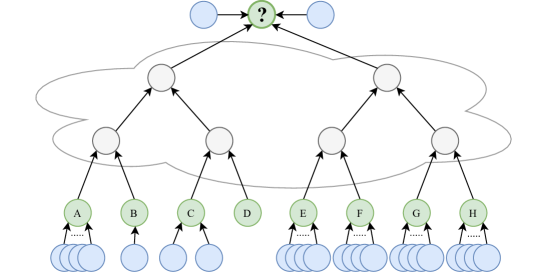
Figure 5: An example of a Tree-NeighborsMatch, that is an instance of the general NeighborsMatch problem that we examine in Section 4. The target node ( ) is the root of a tree of $depth$$=$$3$ (from the target node to the green nodes). The green nodes ( , , , …) have blue neighbors ( ) and an alphabetical label. The node has a single blue neighbor; the node has two blue neighbors; and the node has no blue neighbors; each other green node has another unique number of blue neighbors. The goal it to predict a label for the target node ( ) according to its number of blue neighbors. The correct answer is C in this example, because the target node has two blue neighbors, like the green node that is marked with C in the same graph. To make a correct prediction, the network must propagate information from all leaves toward the target node, and make the decision given a single fixed-sized vector that compresses all this information.

Tree-NeighborsMatch From the perspective of a single node $v$, the rest of the graph may look like a tree of height $K$, rooted at $v$ Xu et al. [2018], Garg et al. [2020]. To simulate this exponentially-growing receptive field, we created an instance of the general NeighborsMatch problem that we described in Section 3 and portrayed in Figure 2. We instantiated the subgraph in the middle of the graph (marked as in Figure 2) as a binary tree of depth $depth$ where the green nodes are its leaves, and the target node is the tree’s root. All edges are directed toward the root, such that information is propagated from all nodes toward the target node. The goal, as in Section 3, is to predict a label for the target node, where the correct answer is the label of the green node that has the same number of blue neighbors as the target node. An illustration is shown in Figure 5 in the appendix. This allows us to control the problem radius, i.e., $r=depth$. In this section we observe the bottleneck empirically; in Section 5 we provide a lower bound for the GNN’s hidden size given $r$.

Model We implemented a network with $r$$+$$1$ graph layers to allow an additional nonlinearity after the information from the leaves reaches the target node. Our PyTorch Geometric Fey and Lenssen [2019] implementation is available at https://github.com/tech-srl/bottleneck/. Our training configuration and hyperparameter ranges are detailed in Appendix A.

Figure 3: Accuracy across problem radius (tree depth) in the NeighborsMatch problem. Over-squashing starts to affect GCN and GIN even at $r=4$.

Results Figure 3 shows the following surprising results: some GNNs fail to fit the dataset starting from $r$$=$$4$. For example, the training accuracy of GCN Kipf and Welling [2017] at $r$$=$$4$ is 70%. At $r$$=$$5$, all GNNs fail to perfectly fit the data. Starting from $r$$=$$4$, the models suffered from over-squashing that resulted in underfitting: the bottleneck prevented the models from distinguishing between different training examples, even after they were observed tens of thousands of times. These results clearly show the existence of over-squashing, starting from $r$$=$$4$.

Why did some GNNs perform better than others? GCN and GIN managed to perfectly fit $r$$=$$3$ at most, while GGNN and GAT also reached 100% accuracy at $r$$=$$4$. This difference can be explained by their neighbor aggregation computation: consider the target node that receives messages in the $r$’th step. GCN and GIN aggregate all neighbors before combining them with the target node’s representation; they thus must compress the information flowing from all leaves into a single vector, and only afterward interact with the target node’s own representation (Equations 2 and 3). In contrast, GAT uses attention to weight incoming messages given the target’s representation: at the last layer only, the target node can ignore the irrelevant incoming edge, and absorb only the relevant incoming edge, which contains information flowing from half of the leaves. That is, a single vector compresses only half of the information. Since the number of leaves grows exponentially with $r$, it is expected that GNNs that need to compress only half of the information (GGNN and GAT) will succeed at an $r$ that is larger by 1. Following Levy et al. [2018], we hypothesize that the GRU cell in GGNNs filters incoming edges as GAT, but perform this filtering as element-wise attention.

If all GNNs have reached low training accuracy, how do GNN-based models usually do fit the training data in public datasets of long-range problems? We hypothesize that they overfit short-range signals and artifacts from the training set, rather than learning the long-range information that was squashed in the bottleneck, and thus generalize poorly at test time.

4.2 Quantum Chemistry: QM9

We wish to measure over-squashing in existing models. But, how can we measure over-squashing? Instead, we measure whether breaking the bottleneck improves the results of long-range problems.

Adding a fully-adjacent layer (FA) In Sections 4.2, 4.3 and 4.4, we took extensively tuned models from previous work, and modified adjacency in the last layer: given a GNN with $K$ layers, we modified the $K$-th layer to be a fully-adjacent layer (FA). A fully-adjacent layer is a GNN layer in which every pair of nodes is connected by an edge. In terms of Equations 1, 2 and 3, converting an existing layer to be fully-adjacent means that $\mathcal{N}_{v}\coloneqq\mathcal{V}$ for every node $v\in\mathcal{V}$, in that layer only. This does not change the type of layer nor add weights, but only changes adjacency of a data sample in a single layer. Thus, the $K-1$ graph layers exploit the graph structure using their original sparse topology, and only the $K$-th layer is an FA layer that allows the topology-aware node-representations to interact directly and consider nodes beyond their original neighbors. Hopefully, this would ease information flow, prevent over-squashing, and reduce the effect of the previously-existed bottleneck. We re-trained the models using the authors’ original code, without performing any additional tuning, to rule out hyperparameter tuning as the source of improvement. Statistics of all datasets can be found in Appendix D.

We note that an FA layer is a simple solution. Its purpose is merely to demonstrate that over-squashing in GNNs is so prevalent and untreated that even the simplest solution helps. Our main contribution is not the solution, but rather, highlighting and explaining the over-squashing problem. This simple solution opens the path for a variety of follow-up improvements and solutions for over-squashing.

Data The QM9 dataset Ramakrishnan et al. [2014], Gilmer et al. [2017], Wu et al. [2018] contains ~130,000 graphs with ~18 nodes. Each graph is a molecule where nodes are atoms, and undirected, typed edges are different types of bonds between the atoms. The goal is to regress each graph to 13 real-valued quantum chemical properties such as dipole moment and isotropic polarizability.

Models We modified the implementation of Brockschmidt [2020] who performed an extensive hyperparameter tuning for multiple GNNs, by searching over 500 configurations; we took the same splits and their best-found configurations. For most GNNs, Brockschmidt found that the best results are achieved using $K$$=$$8$ layers. This hints that this problem depends on long-range information and relies on both graph structure and distant nodes. We re-trained each modified model for each target property using the same code, configuration, and training scheme as Brockschmidt [2020], training each model five times (using different random seeds) for each target property task. We compare the “base” models, reported by Brockschmidt, with our modified and re-trained “$+$FA” models.

	R-GIN			R-GAT			GGNN
Property	base†	$+$FA		base†	$+$FA		base†	$+$FA
mu	2.64$\pm$0.11	2.54$\pm$0.09		2.68$\pm$0.06	2.73$\pm$0.07		3.85$\pm$0.16	3.53$\pm$0.13
alpha	4.67$\pm$0.52	2.28$\pm$0.04		4.65$\pm$0.44	2.32$\pm$0.16		5.22$\pm$0.86	2.72$\pm$0.12
HOMO	1.42$\pm$0.01	1.26$\pm$0.02		1.48$\pm$0.03	1.43$\pm$0.02		1.67$\pm$0.07	1.45$\pm$0.04
LUMO	1.50$\pm$0.09	1.34$\pm$0.04		1.53$\pm$0.07	1.41$\pm$0.03		1.74$\pm$0.06	1.63$\pm$0.06
gap	2.27$\pm$0.09	1.96$\pm$0.04		2.31$\pm$0.06	2.08$\pm$0.05		2.60$\pm$0.06	2.30$\pm$0.05
R2	15.63$\pm$1.40	12.61$\pm$0.37		52.39 $\pm$42.5	15.76$\pm$1.17		35.94$\pm$35.7	14.33$\pm$0.47
ZPVE	12.93$\pm$1.81	5.03$\pm$0.36		14.87$\pm$2.88	5.98$\pm$0.43		17.84$\pm$3.61	5.24$\pm$0.30
U0	5.88$\pm$1.01	2.21$\pm$0.12		7.61$\pm$0.46	2.19$\pm$0.25		8.65$\pm$2.46	3.35$\pm$1.68
U	18.71$\pm$23.36	2.32$\pm$0.18		6.86$\pm$0.53	2.11$\pm$0.10		9.24$\pm$2.26	2.49$\pm$0.34
H	5.62$\pm$0.81	2.26$\pm$0.19		7.64$\pm$0.92	2.27$\pm$0.29		9.35$\pm$0.96	2.31$\pm$0.15
G	5.38$\pm$0.75	2.04$\pm$0.24		6.54$\pm$0.36	2.07$\pm$0.07		7.14$\pm$1.15	2.17$\pm$0.29
Cv	3.53$\pm$0.37	1.86$\pm$0.03		4.11$\pm$0.27	2.03$\pm$0.14		8.86$\pm$9.07	2.25$\pm$0.20
Omega	1.05$\pm$0.11	0.80$\pm$0.04		1.48$\pm$0.87	0.73$\pm$0.04		1.57$\pm$0.53	0.87$\pm$0.09
Relative:		-39.54%			-44.58%			-47.42%

Table 1: Average error rates (5 runs $\pm$ stdev for each property) on the QM9 dataset. The best result for every property in every GNN type is highlighted in bold. Results marked with ${\dagger}$ were previously reported by Brockschmidt [2020] and reproduced by us.

Results Results for the top GNNs are shown in Table 1. The main results are that breaking the bottleneck by modifying a single layer to be an FA layer significantly reduces the error rate, by 42% on average, across six GNN types. These experiments clearly show evidence for a bottleneck in the original GNN models. Results for the other GNNs are shown in Appendix B due to space limitation.

Over-squashing or under-reaching? Barceló et al. [2020] discuss the inability of a GNN node to observe nodes that are farther away than the number of layers $K$. We denote this limitation as under-reaching: for every fixed number of layers $K$, local information cannot travel farther than distance $K$ along edges. So, was the improvement of the FA layer in Table 1 achieved thanks to the reduction in over-squashing, or did the FA layer only extend the nodes’ reachability and prevent under-reaching? To answer this, we measured the graphs’ diameter in the QM9 dataset – the maximum shortest path between any two nodes in a graph. We found that the average diameter is $6.35$$\pm$$0.91$, the maximum diameter is $10$, and the 90’th percentile is $8$, while most models were trained with $K$$=$$8$ layers. That is, at least 90% of the examples in the dataset certainly did not suffer from under-reaching, because the number of layers was greater or equal than their diameter. We trained another set of models with 10 layers, which did not show an improvement over the base models. We conclude that the source of improvement was clearly not the increased reachability, but instead, the reduction in over-squashing.

Can larger hidden sizes achieve a similar improvement? We trained another set of models with doubled dimensions. These models achieved only 5.5% improvement over the base model (Section B.2), while adding the FA layer achieved 42% improvement using the original dimensions and without adding weights. Consistently, in Section 5 we present an analysis that shows how dimensionality increase is ineffective in preventing over-squashing.

Is the entire FA layer needed? We experimented with using only a sampled fraction of edges in the FA layer. As Section B.3 shows, the fraction of added edges in the last layer correlates with the decrease in error. For example, using only half of the possible edges in the last layer (a “semi-adjacent” layer) still reduces the error rate by 31.5% on average compared to “base”.

If all GNNs benefitted from direct interaction between all nodes, maybe the graph structure is not even needed? We trained another set of models (Section B.2) where all $K$ layers are FA layers, thus ignoring the original graph topology; these models produced 1500% higher (worse) error.

4.3 Biological Benchmarks

Data The NCI1 dataset Wale et al. [2008] contains 4110 graphs with ~30 nodes on average, and its task is to predict whether a biochemical compound contains anti-lung-cancer activity. ENZYMES Borgwardt et al. [2005] contains 600 graphs with ~36 nodes on average, and its task is to classify an enzyme to one out of six classes. We used the same 10-folds and split as Errica et al. [2020].

Models We used the implementation of Errica et al. [2020] who performed a fair and thorough comparison between GNNs. The final reported result is the average of 30 test runs (10 folds$\times$3 random seeds). Additional training details are provided in Appendix C.

In ENZYMES, Errica et al. found that a baseline that does not use the graph topology at all (“No Struct”) performs better than all GNNs. In NCI1, GIN performed best. We converted the last layer into an FA layer by modifying the implementation of Errica et al., and repeated the same training procedure. We compare the “base” models from Errica et al. with our re-trained “+FA” models.

		NCI1	ENZYMES
No Struct†		69.8$\pm$2.2	65.2$\pm$6.4
DiffPool	base†	76.9$\pm$1.9	59.5$\pm$5.6
	$+$FA	77.6$\pm$1.3	65.7$\pm$4.8
GraphSAGE	base†	76.0$\pm$1.8	58.2$\pm$6.0
	$+$FA	77.7$\pm$1.8	60.8$\pm$4.5
DGCNN	base†	76.4$\pm$1.7	38.9$\pm$5.7
	$+$FA	76.8$\pm$1.5	42.8$\pm$5.3
GIN	base†	80.0$\pm$1.4	59.6$\pm$4.5
	$+$FA	81.5$\pm$1.2	67.7$\pm$5.3

Table 2: Average accuracy (30 runs$\pm$stdev) on the biological datasets. ${\dagger}$ – previously reported by Errica et al. [2020].

		SeenProj	UnseenProj
GGNN†	base†	85.7$\pm$0.5	79.3$\pm$1.2
	$+$FA	86.3$\pm$0.7	79.1$\pm$1.1
R-GCN	base†	88.3$\pm$0.4	82.9$\pm$0.8
	$+$FA	88.4$\pm$0.7	83.8$\pm$1.0
R-GIN	base†	87.1$\pm$0.1	81.1$\pm$0.9
	$+$FA	87.5$\pm$0.7	81.7$\pm$1.2
GNN-MLP	base†	86.9$\pm$0.3	81.4$\pm$0.7
	$+$FA	87.3$\pm$0.2	81.2$\pm$0.5
R-GAT	base†	86.9$\pm$0.7	81.2$\pm$0.9
	$+$FA	87.9$\pm$1.0	82.0$\pm$1.9

Table 3: Average accuracy (5 runs$\pm$stdev) on VarMisuse. ${\dagger}$ – previously reported by Brockschmidt [2020].

Results Results are shown in Table 2. The main results are as follows: (a) in NCI1, GIN+FA improves by 1.5% over GIN-base, which was previously the best performing model; (b) in ENZYMES, where Errica et al. [2020] found that none of the GNNs exploit the topology of the graph, we find that GIN+FA does exploit the structure and improves by 8.1% over GIN-base and by 2.5% over No Struct. On average, models with FA layers relatively reduce the error rate by 12% in ENZYMES and by 4.8% in NCI1. These experiments clearly show evidence for a bottleneck in the original GNN models.

4.4 Programs: VarMisuse

Data VarMisuse Allamanis et al. [2018] is a node-prediction problem that depends on long-range information in computer programs. We used the same splits as Allamanis et al. [2018].

Models We use the implementation of Brockschmidt [2020] who performed an extensive hyperparameter tuning by searching over 30 configurations for each GNN type. The best results were found using 6-10 layers, which hints that this problem requires long-range information. We modified the last layer to be an FA layer, and used the resulting representations for node classification. We used the same best found configurations as Brockschmidt [2020] add re-trained each model five times.

Results Results are shown in Table 3. The main result is that adding an FA layer to all GNNs improves their SeenProjTest accuracy, obtaining a new state-of-the-art of 88.4%. In the UnseenProjTest set, adding an an FA layer improves the results of some of most of the GNNs, obtaining a new state-of-the-art of 83.8%. These improvements are significant, especially since they were achieved on extensively tuned models, without any further tuning by us.

5 How Long is Long-Range?

Figure 4: Combinatorial and empirical lower bounds of the model dimension given the problem radius.

In this section, we analyze over-squashing combinatorially in the Tree-NeighborsMatch problem. We provide a combinatorial lower bound for the minimal hidden size that a GNN requires to perfectly fit the data (learn to 100% training accuracy) given its problem radius $r$. We denote the arity of such a tree by $m$ ($=$$2$ in our experiments); the counting base as $b$$=$$2$; the number of bits in a floating-point variable as $f$$=$$32$; and the hidden dimension of the GNN, i.e., the size of a node vector $\mathbf{h}_{v}^{\left(k\right)}$, as $d$.

A full tree of arity $m$ and problem radius $r$$=$$depth$ has $m^{r}$ green label-nodes. All $\left(m^{r}\right)!$ possible permutations of the labels {A, B, C, …} are valid, disregarding the order of sibling nodes. Thus, the number of label assignments of green nodes is $\left(m^{r}\right)!/\left(m!\right)^{m^{r}-1}$ (there are $m^{r}-1$ parent nodes, where the order of each of their $m$ siblings can be permutated). Right before interacting with the target node and predicting the label, a single vector of size $d$ must encapsulate the information flowing from all green nodes (Equations 2 and 3). Such a vector contains $d$ floating-point elements, each of them is stored as $f$ bits. Overall, the number of possible cases that this vector can distinguish between is $b^{f\cdot d}$. The number of possible cases that the vector can distinguish between must be greater than the number of different examples that this vector may encounter in the training data. This requirement is expressed in Equation 4. Considering binary trees ($m$$=$$2$), and floating-point values of $f$$=$$32$ binary ($b$$=$$2$) bits, we get Equation 5:

$$b^{f\cdot d}>\frac{\left(m^{r}\right)!}{\left(m!\right)^{m^{r}-1}}$$ (4)

$$2^{32\cdot d}>\frac{\left(2^{r}\right)!}{2^{2^{r}-1}}$$ (5)

Since factorial grows faster than an exponent with a constant base, a small increase in $r$ requires a much larger increase in $d$. Specifically, for $d$$=$$32$ as in the experiments in Section 4.1, the maximal problem radius is as low as $r$$=$$7$. That is, a model with $d$$=$$32$ cannot obtain 100% accuracy for $r$$>$$7$.

In practice, the problem is worse; i.e., the empirical minimal $d$ is higher than the combinatorial, because even if a solution to storing some information in a vector of a certain size exists, a gradient descent-based algorithm is not guaranteed to find it. Figure 4 shows the combinatorial lower bound of $d$ given $r$. We also repeated the experiments from Section 4.1 and report the minimal empirical $d$ for each value of $r$. As shown in Figure 4, the empirical and the theoretical minimal $d$ grow exponentially with $r$; for example, even $d$$=$$512$ can empirically fit $r$$=$$7$ at most.

6 Related Work

Under-reaching Barceló et al. [2020] found that the expressiveness of GNNs captures only a small fragment of first-order logic. The main limitation arises from the inability of a node to be aware of nodes that are farther away than the number of layers $K$, while the existence of such nodes can be easily described using logic. We denote this limitation as under-reaching. Nevertheless, even when information is reachable within $K$ edges, we show that this information might be over-squashed along the way. Thus, the over-squashing limitation described in this paper is tighter than under-reaching.

Over-smoothing As observed before, node representations become indistinguishable and prediction performance severely degrades as the number of layers increases. The accepted explanation to this phenomenon is over-smoothing Li et al. [2018], Wu et al. [2020], Oono and Suzuki [2020]. This might explain the empirical optimality of few layers in short-range tasks (e.g., only $K$$=$$2$ layers in Kipf and Welling [2017]). Nonetheless, some problems depend on longer-range information propagation and thus require more layers, to avoid under-reaching. We hypothesize that in long-range problems, the explanation for the degraded performance is over-squashing rather than over-smoothing. For further discussion of over-smoothing vs. over-squashing, see Appendix E.

Avoiding over-squashing Some previous work avoid over-squashing by various profitable means: Gilmer et al. [2017] add “virtual edges” to shorten long distances; Scarselli et al. [2008] add “supersource nodes”; and Allamanis et al. [2018] designed program analyses that serve as 16 “shortcut” edge types. However, none of these explicitly explained these solutions using over-squashing, and did not identify the bottleneck and its negative cross-domain implications.

7 Conclusion

We propose a novel explanation to a well known limitation in training graph neural networks: a bottleneck that causes over-squashing. Problems that depend on long-range interaction require as many GNN layers as the desired radius of each node’s receptive field. This causes an exponentially-growing amount of information to be squashed into a fixed-length vector. As a result, the GNN fails to propagate long-range information, learns only short-range signals from the training data instead, and performs poorly when the prediction task depends on long-range interaction.

We demonstrate the existence of the bottleneck in a controlled problem, provide theoretical lower bounds for the hidden size given the problem radius, and show that GCN and GIN are more susceptible to over-squashing than GAT and GGNN. We further show that prior models of chemical, biological and programmatical benchmarks suffer from over-squashing by showing that they can be dramatically improved using a simple FA layer. We conclude that over-squashing in GNNs is so prevalent and untreated in some benchmarks – that even the simplest solution helps. Our observations open the path for a variety of follow-up improvements and even better solutions for over-squashing.

Appendix A Tree-NeighborsMatch – Training Details

Data

We created a separate dataset for every tree depth (which is equal to $r$, the problem radius) and sampled up to 32,000 examples per dataset. The label of each leaf (“A”, “B”, “C” in Figure 2) is represented as a one-hot vector. To tease the effect of the bottleneck from the ability of a GNN to count neighbors, we concatenated each leaf node’s initial representation with a 1-hot vector representing the number of blue neighbors, instead of creating the blue nodes. The target node is initialized with a learned vector as its (missing) label, concatenated with a 1-hot vector representing its number of blue neighbors. Intermediate nodes are initialized with another learned vector.

Model

The network has an initial linear layer, followed by $r+1$ GNN layers. Afterward, the final target node representation goes through a linear layer and a softmax to predict its label. We experimented with GCN Kipf and Welling [2017], GGNN Li et al. [2016], GIN Xu et al. [2019] and GAT Veličković et al. [2018] as the graph layers.

In Section 4.1, we used model dimensions of $d$$=$$32$. Larger values led to the exact same trend. We added residual connections, summing every node with its own representation in the previous layer to increase expressivity, and layer normalization which eased convergence. We used the Adam optimizer with a learning rate of $10^{-3}$, decayed by $0.5$ after every 1000 epochs without an increase in training accuracy, and stopped training after 2000 epochs of no training accuracy improvement. This usually led to tens of thousands of training epochs, sometimes reaching 100,000 epochs.

To rule out hyperparameter tuning as the source of degraded performance, we experimented with changing activations (ReLu, tanh, MLP, none), using layer normalization and batch normalization, residual connections, various batch sizes, and whether or not the same GNN weights should be “unrolled” over time steps. The presented results were obtained using the configurations that achieved the best results.

Over-squashing or just long-range? To rule out the possibility that the long-range itself is preventing the GNNs from fitting the data, we repeated the experiment of Figure 3 for depths 4 to 8, where the distance between the leaves and the target node remained the same, but the amount of over-squashing was as in $r$$=$$2$. That is, the graph looks like a tree of $depth$$=$$2$, where the root is connected to a “chain” of length of up to 6, and the target node is at the other side of the chain. This setting maintains the long-range as in the original problem, but reduces the amount of information that needs to be squashed. In other words, This setting disentangles of the effect of the long-range itself from the effect of the growing amount of information (i.e., from over-squashing). In this setting, all GNN types managed to easily fit the data to close to 100% across all distances, showing that the problem is the amount of over-squashing, rather than the long-range itself.

	MLP			R-GCN			GNN-FiLM
Property	base†	$+$FA		base†	$+$FA		base†	$+$FA
mu	2.36$\pm$0.04	2.19$\pm$0.04		3.21$\pm$0.06	2.92$\pm$0.07		2.38$\pm$0.13	2.26$\pm$0.06
alpha	4.27$\pm$0.36	1.92$\pm$0.06		4.22$\pm$0.45	2.14$\pm$0.08		3.75$\pm$0.11	1.93$\pm$0.08
HOMO	1.25$\pm$0.04	1.19$\pm$0.04		1.45$\pm$0.01	1.37$\pm$0.02		1.22$\pm$0.07	1.11$\pm$0.01
LUMO	1.35$\pm$0.04	1.20$\pm$0.05		1.62$\pm$0.04	1.41$\pm$0.01		1.30$\pm$0.05	1.21$\pm$0.05
gap	2.04$\pm$0.05	1.82$\pm$0.05		2.42$\pm$0.14	2.03$\pm$0.03		1.96$\pm$0.06	1.79$\pm$0.07
R2	14.86$\pm$1.62	12.40$\pm$0.84		16.38$\pm$0.49	13.55$\pm$0.50		15.59$\pm$1.38	11.89$\pm$0.73
ZPVE	12.00$\pm$1.66	4.68$\pm$0.29		17.40$\pm$3.56	5.81$\pm$0.61		11.00$\pm$0.74	4.68$\pm$0.49
U0	5.55$\pm$0.38	1.71$\pm$0.13		7.82$\pm$0.80	1.75$\pm$0.18		5.43$\pm$0.96	1.60$\pm$0.12
U	6.20$\pm$0.88	1.72$\pm$0.12		8.24$\pm$1.25	1.88$\pm$0.22		5.95$\pm$0.46	1.75$\pm$0.08
H	5.96$\pm$0.45	1.70$\pm$0.08		9.05$\pm$1.21	1.85$\pm$0.18		5.59$\pm$0.57	1.93$\pm$0.42
G	5.09$\pm$0.57	1.53$\pm$0.15		7.00$\pm$1.51	1.76$\pm$0.15		5.17$\pm$1.13	1.77$\pm$0.05
Cv	3.38$\pm$0.20	1.69$\pm$0.08		3.93$\pm$0.48	1.90$\pm$0.07		3.46$\pm$0.21	1.64$\pm$0.10
Omega	0.84$\pm$0.02	0.63$\pm$0.04		1.02$\pm$0.05	0.75$\pm$0.04		0.98$\pm$0.06	0.69$\pm$0.05
Relative:		-40.33%			-43.40%			-39.53%

Table 4: Average error rates and standard deviations on the QM9 targets. Best result for every property in every GNN type is highlighted in bold. Results marked with ${\dagger}$ were previously reported by Brockschmidt [2020].

Appendix B QM9 – Additional Results

B.1 Additional GNN Types

Because of space limitations, in Section 4.2 we presented results on the QM9 dataset only for R-GIN, R-GAT and GGNN. In this section, we show that additional GNN architectures benefit from breaking the bottleneck using a fully-adjacent layer: GNN-MLP , R-GCN Schlichtkrull et al. [2018] and GNN-FiLM Brockschmidt [2020].

All experiments were performed using the extensively-tuned implementation of Brockschmidt [2020] who experimented with over 500 hyperparameter configurations.

Table 4 contains additional results for GGNN, R-GCN and R-GIN. As shown in Table 4, adding an FA layer significantly improves results across all GNN architectures, for all properties.

B.2 Alternative Solutions

Table 5 shows additional experiments, all performed using GCN. base^† is the original model of Brockschmidt [2020] as in Table 4. $+$FA is the model that we re-trained with the last layer modified to an FA layer.

$2$$\times$$d$ is a model that was trained with a doubled hidden dimension size, $d=256$ instead of $d=128$ as in the base model. As shown, doubling the hidden dimension size leads to a small improvement of only 5.5% reduction in error. In comparison, the $+$FA model used the original dimension sizes and achieves a much larger improvement of 43.40%.

All FA is a model that was trained with all GNN layers converted into FA layers, practically ignoring the graph topology. This led to much worse results of more than 1500% higher error. This shows that the graph topology is important in this benchmark, and that a direct interaction between nodes (as in a single FA layer) must be performed in addition to considering the topology.

$2\times$FA is a model where the last layer was modified into an FA layer, and an additional FA layer was stacked on top of it. This led to results that are very similar to $+$FA.

Penultimate FA is a model where the FA layer is the penultimate layer (the $K-1$-th), followed by a standard GNN layer as the $K$-th layer. This led to results that are even slightly better than $+$FA.

Property	base†	$+$FA	$2$$\times$$d$	All FA	$2\times$FA	Penultimate FA
mu	3.21$\pm$0.06	2.92$\pm$0.07	2.99$\pm$0.08	11.52	2.89$\pm$0.08	2.80$\pm$0.08
alpha	4.22$\pm$0.45	2.14$\pm$0.08	3.57$\pm$0.40	9.19	2.23$\pm$0.04	2.14$\pm$0.10
HOMO	1.45$\pm$0.01	1.37$\pm$0.02	1.36$\pm$1.87	9.95	1.39$\pm$0.02	1.34$\pm$0.03
LUMO	1.62$\pm$0.04	1.41$\pm$0.01	1.43$\pm$0.04	19.13	1.42$\pm$0.04	1.37$\pm$0.02
gap	2.42$\pm$0.14	2.03$\pm$0.03	2.33$\pm$0.23	24.62	2.06$\pm$0.05	2.00$\pm$0.03
R2	16.38$\pm$0.49	13.55$\pm$0.50	18.4$\pm$0.76	168.09	13.97$\pm$0.56	12.92$\pm$0.11
ZPVE	17.40$\pm$3.56	5.81$\pm$0.61	15.8$\pm$2.59	591.33	5.79$\pm$0.50	4.53$\pm$0.62
U0	7.82$\pm$0.80	1.75$\pm$0.18	7.60$\pm$2.07	188.59	1.90$\pm$0.1	1.98$\pm$0.25
U	8.24$\pm$1.25	1.88$\pm$0.22	7.65$\pm$1.51	189.72	1.71$\pm$0.16	2.05$\pm$0.23
H	9.05$\pm$1.21	1.85$\pm$0.18	8.67$\pm$1.10	191.11	1.83$\pm$0.11	1.73$\pm$0.14
G	7.00$\pm$1.51	1.76$\pm$0.15	2.90$\pm$1.15	173.68	1.93$\pm$0.11	1.96$\pm$0.42
Cv	3.93$\pm$0.48	1.90$\pm$0.07	3.99$\pm$0.07	64.18	1.90$\pm$0.14	1.83$\pm$0.11
Omega	1.02$\pm$0.05	0.75$\pm$0.04	1.03$\pm$0.54	23.89	0.69$\pm$0.06	0.67$\pm$0.01
relative	0.0%	-43.40%	-5.50%	+1520%	-43.30%	-45.2%

Table 5: Average error rates and standard deviations on the QM9 targets with GCN using alternative solutions.

	base†	0.25$\times$ FA	0.5$\times$ FA	0.75$\times$ FA	$+$FA (as in Table 4)
Avg. error compared to base†	-0%	-8.4%	-31.5%	-37.1%	-43.4%

Table 6: Average error rates and standard deviations on the QM9 targets with GCN, where we use only a fraction of the edges in the FA layer.

B.3 Partial-FA Layers

We also examined whether instead of adding a “full fully-adjacent layer”, we can randomly sample only a fraction of these edges. We randomly sampled only $\{0.25,0.5,0.75\}$ of the edges in the full FA layer in every example, and trained the model for each target property 5 times. Table 6 shows the results of these experiments using GCN. base^† is the original model of Brockschmidt [2020] as in Table 4. $+$FA is the model that we re-trained with the last layer modified to an FA layer. $\{0.25,0.5,0.75\}\times$ FA are the models were only a fraction of the edges in the FA layer were used.

As shown in Table 6, the full FA layer achieves the largest reduction in error (-43.4%), but even adding a fraction of the edges improves the results over the base model. For example, using only half of the edges (0.5$\times$ FA) reduces the error by 31.5%. Overall, the percentage of used edges in the partial-FA layer is correlated with its reduction in error.

Appendix C Biological Benchmarks – Training Details

We used the implementation of Errica et al. [2020] who performed a fair and thorough comparison between GNNs, by splitting each dataset to 10-folds; then, for each GNN type they select a configuration among a grid of 72 configurations according to the validation set; finally, the best configuration for each fold is trained three additional times, early stopped using the validation set, and evaluated on the test set. The final reported result is the average of all 30 test runs (10-folds$\times$3). The final standard deviation is computed among the average results of each of the ten folds.

Appendix D Data Statistics

D.1 Synthetic Dataset: Tree-NeighborsMatch

Statistics of the synthetic Tree-NeighborsMatch dataset are shown in Table 7.

Table 7: The number of examples, in our experiments and combinatorially, for every value of $depth$.

$depth$	# Training examples sampled	Total combinatorial: $\left(2^{depth}!\right)\cdot 2^{depth}$
2	96	96
3	8000	$>3\cdot 10^{5}$
4	16,000	$>3\cdot 10^{14}$
5	32,000	$>10^{36}$
6	32,000	$>10^{90}$
7	32,000	$>10^{217}$
8	32,000	$>10^{509}$

D.2 Quantum Chemistry: QM9

Statistics of the quantum chemistry QM9 dataset, as used in Brockschmidt [2020] are shown in Table 8.

Table 8: Statistics of the QM9 chemical dataset Ramakrishnan et al. [2014] as used by Brockschmidt [2020].

	Training	Validation	Test
# examples	110,462	10,000	10,000
# nodes - average	18.03	18.06	18.09
# nodes - standard deviation	2.9	2.9	2.9
# edges - average	18.65	18.67	18.72
# edges - standard deviation	3.1	3.1	3.1

D.3 Biological Benchmarks

Statistics of the biological datasets, as used in Errica et al. [2020], are shown in Table 9.

Table 9: Statistics of the biological datasets, as used by Errica et al. [2020].

	NCI1 Wale et al. [2008]	ENZYMES Borgwardt et al. [2005]
# examples	4110	600
# classes	2	6
# nodes - average	29.87	32.63
# nodes - standard deviation	13.6	15.3
# edges - average	32.30	64.14
# edges - standard deviation	14.9	25.5
# node labels	37	3

D.4 VarMisuse

Statistics of the VarMisuse dataset, as used in Allamanis et al. [2018] and Brockschmidt [2020], are shown in Table 10.

Table 10: Statistics of the VarMisuse dataset Allamanis et al. [2018] as used by Brockschmidt [2020].

	Training	Validation	UnseenProject Test	SeenProject Test
# graphs	254360	42654	117036	59974
# nodes - average	2377	1742	1959	3986
# edges - average	7298	7851	5882	12925

Appendix E Discussion: Over-Smoothing vs. Over-Squashing

Although over-smoothing and over-squashing are related, they are disparate phenomena that occur in different types of problems. For example, imagine a triangular graph containing only three nodes, where every node has a scalar value, an edge to each of the other nodes, and needs to compute a function of its own value and the other nodes’ values. The problem radius $r$ in this case is $r$$=$$1$. As we increase the number of layers, the representations of the nodes might become indistinguishable, and thus suffer from over-smoothing. However, there will be no over-squashing in this case, because there is no growing amount of information that is squashed into fixed-sized vectors while passing long-range messages. Contrarily, in the Tree-NeighborsMatch problem, there is no reason for over-smoothing to occur, because there are no two nodes that can converge to the same representation. A node in a “higher” level in the tree contains twice the information than a node in a “lower” level. Thus, this is a case where over-squashing can occur without over-smoothing.

References

- Allamanis et al. [2018] Miltiadis Allamanis, Marc Brockschmidt, and Mahmoud Khademi. Learning to represent programs with graphs. In International Conference on Learning Representations, 2018. URL https://openreview.net/forum?id=BJOFETxR-.
- Barceló et al. [2020] Pablo Barceló, Egor V. Kostylev, Mikael Monet, Jorge Pérez, Juan Reutter, and Juan Pablo Silva. The logical expressiveness of graph neural networks. In International Conference on Learning Representations, 2020. URL https://openreview.net/forum?id=r1lZ7AEKvB.
- Borgwardt et al. [2005] Karsten M Borgwardt, Cheng Soon Ong, Stefan Schönauer, SVN Vishwanathan, Alex J Smola, and Hans-Peter Kriegel. Protein function prediction via graph kernels. Bioinformatics, 21(suppl_1):i47–i56, 2005.
- Brockschmidt [2020] Marc Brockschmidt. Gnn-film: Graph neural networks with feature-wise linear modulation. Proceedings of the 36th International Conference on Machine Learning, ICML, 2020.
- Chen et al. [2020a] Deli Chen, Yankai Lin, Wei Li, Peng Li, Jie Zhou, and Xu Sun. Measuring and relieving the over-smoothing problem for graph neural networks from the topological view. In Proceedings of the Thirty-Fourth Conference on Association for the Advancement of Artificial Intelligence (AAAI), 2020a.
- Chen et al. [2018] Jianfei Chen, Jun Zhu, and Le Song. Stochastic training of graph convolutional networks with variance reduction. In International Conference on Machine Learning, pages 942–950, 2018.
- Chen et al. [2020b] Ming Chen, Zhewei Wei, Zengfeng Huang, Bolin Ding, and Yaliang Li. Simple and deep graph convolutional networks. In International Conference on Machine Learning, pages 1725–1735. PMLR, 2020b.
- Cho et al. [2014a] Kyunghyun Cho, Bart van Merriënboer, Dzmitry Bahdanau, and Yoshua Bengio. On the properties of neural machine translation: Encoder–decoder approaches. In Proceedings of SSST-8, Eighth Workshop on Syntax, Semantics and Structure in Statistical Translation, pages 103–111, 2014a.
- Cho et al. [2014b] Kyunghyun Cho, Bart Van Merriënboer, Caglar Gulcehre, Dzmitry Bahdanau, Fethi Bougares, Holger Schwenk, and Yoshua Bengio. Learning phrase representations using rnn encoder-decoder for statistical machine translation. arXiv preprint arXiv:1406.1078, 2014b.
- Duvenaud et al. [2015] David K Duvenaud, Dougal Maclaurin, Jorge Iparraguirre, Rafael Bombarell, Timothy Hirzel, Alán Aspuru-Guzik, and Ryan P Adams. Convolutional networks on graphs for learning molecular fingerprints. In Advances in neural information processing systems, pages 2224–2232, 2015.
- Errica et al. [2020] Federico Errica, Marco Podda, Davide Bacciu, and Alessio Micheli. A fair comparison of graph neural networks for graph classification. In International Conference on Learning Representations, 2020. URL https://openreview.net/forum?id=HygDF6NFPB.
- Fey and Lenssen [2019] Matthias Fey and Jan E. Lenssen. Fast graph representation learning with PyTorch Geometric. In ICLR Workshop on Representation Learning on Graphs and Manifolds, 2019.
- Garg et al. [2020] Vikas K Garg, Stefanie Jegelka, and Tommi Jaakkola. Generalization and representational limits of graph neural networks. arXiv preprint arXiv:2002.06157, 2020.
- Gilmer et al. [2017] Justin Gilmer, Samuel S Schoenholz, Patrick F Riley, Oriol Vinyals, and George E Dahl. Neural message passing for quantum chemistry. In Proceedings of the 34th International Conference on Machine Learning-Volume 70, pages 1263–1272. JMLR. org, 2017.
- Gori et al. [2005] Marco Gori, Gabriele Monfardini, and Franco Scarselli. A new model for learning in graph domains. In Proceedings. 2005 IEEE International Joint Conference on Neural Networks, 2005., volume 2, pages 729–734. IEEE, 2005.
- Hamilton et al. [2017] Will Hamilton, Zhitao Ying, and Jure Leskovec. Inductive representation learning on large graphs. In Advances in neural information processing systems, pages 1024–1034, 2017.
- Kipf and Welling [2017] Thomas N Kipf and Max Welling. Semi-supervised classification with graph convolutional networks. In ICLR, 2017.
- Klicpera et al. [2018] Johannes Klicpera, Aleksandar Bojchevski, and Stephan Günnemann. Predict then propagate: Graph neural networks meet personalized pagerank. In International Conference on Learning Representations, 2018.
- Leskovec and Mcauley [2012] Jure Leskovec and Julian J Mcauley. Learning to discover social circles in ego networks. In Advances in neural information processing systems, pages 539–547, 2012.
- Levy et al. [2018] Omer Levy, Kenton Lee, Nicholas FitzGerald, and Luke Zettlemoyer. Long short-term memory as a dynamically computed element-wise weighted sum. In Proceedings of the 56th Annual Meeting of the Association for Computational Linguistics (Volume 2: Short Papers), pages 732–739, 2018.
- Li et al. [2018] Qimai Li, Zhichao Han, and Xiao-Ming Wu. Deeper insights into graph convolutional networks for semi-supervised learning. In Thirty-Second AAAI Conference on Artificial Intelligence, 2018.
- Li et al. [2016] Yujia Li, Daniel Tarlow, Marc Brockschmidt, and Richard Zemel. Gated graph sequence neural networks. In International Conference on Learning Representations, 2016.
- Maron et al. [2019] Haggai Maron, Heli Ben-Hamu, Hadar Serviansky, and Yaron Lipman. Provably powerful graph networks. In Advances in Neural Information Processing Systems, pages 2153–2164, 2019.
- Micheli [2009] Alessio Micheli. Neural network for graphs: A contextual constructive approach. IEEE Transactions on Neural Networks, 20(3):498–511, 2009.
- Morris et al. [2019] Christopher Morris, Martin Ritzert, Matthias Fey, William L Hamilton, Jan Eric Lenssen, Gaurav Rattan, and Martin Grohe. Weisfeiler and leman go neural: Higher-order graph neural networks. In Proceedings of the AAAI Conference on Artificial Intelligence, volume 33, pages 4602–4609, 2019.
- Nikolentzos et al. [2019] Giannis Nikolentzos, George Dasoulas, and Michalis Vazirgiannis. k-hop graph neural networks. ArXiv, abs/1907.06051, 2019.
- Oono and Suzuki [2020] Kenta Oono and Taiji Suzuki. Graph neural networks exponentially lose expressive power for node classification. In International Conference on Learning Representations, 2020. URL https://openreview.net/forum?id=S1ldO2EFPr.
- Ramakrishnan et al. [2014] Raghunathan Ramakrishnan, Pavlo O Dral, Matthias Rupp, and O Anatole Von Lilienfeld. Quantum chemistry structures and properties of 134 kilo molecules. Scientific data, 1:140022, 2014.
- Rong et al. [2020] Yu Rong, Wenbing Huang, Tingyang Xu, and Junzhou Huang. Dropedge: Towards deep graph convolutional networks on node classification. In International Conference on Learning Representations, 2020. URL https://openreview.net/forum?id=Hkx1qkrKPr.
- Scarselli et al. [2008] Franco Scarselli, Marco Gori, Ah Chung Tsoi, Markus Hagenbuchner, and Gabriele Monfardini. The graph neural network model. IEEE Transactions on Neural Networks, 20(1):61–80, 2008.
- Schlichtkrull et al. [2018] Michael Schlichtkrull, Thomas N Kipf, Peter Bloem, Rianne Van Den Berg, Ivan Titov, and Max Welling. Modeling relational data with graph convolutional networks. In European Semantic Web Conference, pages 593–607. Springer, 2018.
- Sen et al. [2008] Prithviraj Sen, Galileo Namata, Mustafa Bilgic, Lise Getoor, Brian Galligher, and Tina Eliassi-Rad. Collective classification in network data. AI magazine, 29(3):93–93, 2008.
- Shchur et al. [2018] Oleksandr Shchur, Maximilian Mumme, Aleksandar Bojchevski, and Stephan Günnemann. Pitfalls of graph neural network evaluation. Relational Representation Learning Workshop, NeurIPS 2018, 2018.
- Sutskever et al. [2014] Ilya Sutskever, Oriol Vinyals, and Quoc V Le. Sequence to sequence learning with neural networks. In Advances in Neural Information Processing Systems, pages 3104–3112, 2014.
- Veličković et al. [2018] Petar Veličković, Guillem Cucurull, Arantxa Casanova, Adriana Romero, Pietro Liò, and Yoshua Bengio. Graph attention networks. In International Conference on Learning Representations, 2018.
- Wale et al. [2008] Nikil Wale, Ian A Watson, and George Karypis. Comparison of descriptor spaces for chemical compound retrieval and classification. Knowledge and Information Systems, 14(3):347–375, 2008.
- Wu et al. [2018] Zhenqin Wu, Bharath Ramsundar, Evan N Feinberg, Joseph Gomes, Caleb Geniesse, Aneesh S Pappu, Karl Leswing, and Vijay Pande. Moleculenet: a benchmark for molecular machine learning. Chemical science, 9(2):513–530, 2018.
- Wu et al. [2020] Zonghan Wu, Shirui Pan, Fengwen Chen, Guodong Long, Chengqi Zhang, and S Yu Philip. A comprehensive survey on graph neural networks. IEEE Transactions on Neural Networks and Learning Systems, 2020.
- Xu et al. [2018] Keyulu Xu, Chengtao Li, Yonglong Tian, Tomohiro Sonobe, Ken-ichi Kawarabayashi, and Stefanie Jegelka. Representation learning on graphs with jumping knowledge networks. In International Conference on Machine Learning, pages 5453–5462, 2018.
- Xu et al. [2019] Keyulu Xu, Weihua Hu, Jure Leskovec, and Stefanie Jegelka. How powerful are graph neural networks? In International Conference on Learning Representations, 2019. URL https://openreview.net/forum?id=ryGs6iA5Km.
- Zhao and Akoglu [2020] Lingxiao Zhao and Leman Akoglu. Pairnorm: Tackling oversmoothing in gnns. In International Conference on Learning Representations, 2020. URL https://openreview.net/forum?id=rkecl1rtwB.