The accretion history of high-mass stars:
An ArTéMiS pilot study of Infrared Dark Clouds

Abstract

The mass growth of protostars is a central element to the determination of fundamental stellar population properties such as the initial mass function. Constraining the accretion history of individual protostars is therefore an important aspect of star formation research. The goal of the study presented here is to determine whether high-mass (proto)stars gain their mass from a compact ($<0.1$ pc) fixed-mass reservoir of gas, often referred to as dense cores, in which they are embedded, or whether the mass growth of high-mass stars is governed by the dynamical evolution of the parsec-scale clump that typically surrounds them. To achieve this goal, we performed a 350$\mu$m continuum mapping of 11 infrared dark clouds, along side some of their neighbouring clumps, with the ArTéMiS camera on APEX. By identifying about 200 compact ArTéMiS sources, and matching them with Herschel Hi-GAL 70$\mu$m sources, we have been able to produce mass vs. temperature diagrams. We compare the nature (i.e. starless or protostellar) and location of the ArTéMiS sources in these diagrams with modelled evolutionary tracks of both core-fed and clump-fed accretion scenarios. We argue that the latter provide a better agreement with the observed distribution of high-mass star-forming cores. However, a robust and definitive conclusion on the question of the accretion history of high-mass stars requires larger number statistics.

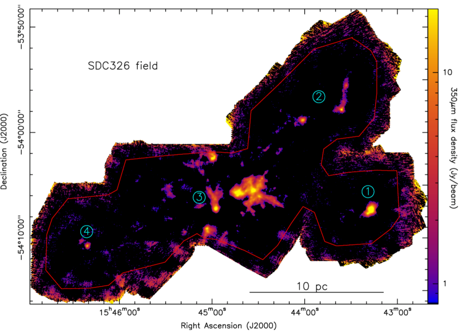
Figure 1: 350$\mu m$ ArTéMiS image of the SDC326 field (in logarithmic scale), that includes 4 targeted IRDCs whose ID numbers (in cyan) correspond to those indicated in Table 1. The area within the red polygone roughly corresponds to the area of uniform noise. The 10 pc bar scale at the bottom of the image assumes a distance of 2.6 kpc.

1 Introduction

Our knowledge about star formation has made tremendous progress in the past few years (André et al., 2014; Motte et al., 2018b). As a result of the science exploitation of Herschel data, our picture of how matter is condensed from diffuse clouds to stars has been significantly improved. In particular, one striking result has been the ubiquity of interstellar filaments in all types of molecular clouds, including low-mass star-forming (André et al., 2010), massive-star forming (Molinari et al., 2010), and even non-star-forming clouds (Men’shchikov et al., 2010). In nearby, and mostly low-mass, star-forming regions nearly all the dense gas ($n_{H_{2}}\geq 10^{4}$ cm^-3; $N_{H_{2}}\geq 10^{22}$ cm^-2) is concentrated within 0.1pc-width filaments (Arzoumanian et al., 2011, 2019). Moreover, the vast majority ($\sim$ 75%) of prestellar cores are found to lie within these filaments (Könyves et al., 2015, 2020; Ladjelate et al., 2020). It has therefore been proposed that solar-type star-forming cores form as the result of Jeans-type gravitational instabilities developing along self-gravitating filaments (Inutsuka & Miyama, 1997), providing a compact and, at least to first order, fixed mass reservoir for the protostars forming inside them. As a result, such protostars are said to be core-fed. This scenario is believed to explain the shape of the prestellar core mass function as observed in a number of low-mass star-forming clouds (e.g. Motte et al., 1998; Könyves et al., 2015), and therefore the origin of the base of the initial mass function (IMF) from $\sim 0.1$ to 5 M_⊙ (cf. André et al., 2014, 2019; Lee et al., 2017).

Table 1: Target properties. The V_lsr column corresponds to velocities that have been obtained using the MALT90 N₂H⁺(1-0) line, with the exception of SDC340.928-1.042 (marked with an asterisk) for which we used the ThrUMMS ¹³CO(1-0) line (see text). IRDCs having several velocities/distances correspond to ArTéMiS maps where several clumps have been detected. Noise values correspond to the median rms noise in each of the 5 observed fields, for both the original ArTéMiS images and the Gaussian filtered ones.

ID#	IRDC name	Coordinates	Vlsr	Distance	Radius	Mass	Unfilt. noise	Filt. noise
		(J2000)	(km/s)	(kpc)	(pc)	(M⊙)	(Jy/beam)	(Jy/beam)
1	SDC326.476+0.706	15:43:16.4 -54:07:13	-40.5	2.7	1.08	3730	0.48	0.26
2	SDC326.611+0.811	15:43:36.3 -53:57:45	-37.0	2.5	1.29	3260	0.48	0.26
3	SDC326.672+0.585	15:44:57.3 -54:07:14	-41.3	2.7	0.91	4120	0.48	0.26
4	SDC326.796+0.386	15:46:20.9 -54:10:44	-20.4	1.6	0.42	240	0.48	0.26
5	SDC328.199-0.588	15:57:59.6 -53:58:01	-44.3 -38.7	2.9 2.6	2.77	33220	0.63	0.41
6	SDC340.928-1.042	16:55:01.4 -45:11:42	-24.1∗	2.3	0.73	640	0.46	0.31
7	SDC340.969-1.020	16:54:57.1 -45:09:04	-24.1	2.3	0.66	2630	0.46	0.31
8	SDC343.722-0.178	17:00:49.6 -42:26:05	-28.0 -26.7 -25.6	2.8 2.7 2.6	1.42	5270	0.51	0.38
9	SDC343.735-0.110	17:00:32.6 -42:25:02	-27.3	2.7	0.45	510	0.51	0.38
10	SDC343.781-0.236	17:01:13.0 -42:27:42	-27.1	2.5	0.46	360	0.51	0.38
11	SDC345.000-0.232	17:05:10.8 -41:29:08	-27.8	2.9	2.14	16160	0.43	0.30

At the high-mass end of the IMF, however, it is well known that thermal Jeans-type fragmentation cannot explain the formation of cores more massive than a few solar masses (e.g. Bontemps et al., 2010). In fact, the search for compact high-mass prestellar cores with ALMA systematically reveals that reasonable candidates identified with single-dish telescopes are systematically sub-fragmented into low-mass cores (e.g. Svoboda et al., 2019; Sanhueza et al., 2019; Louvet et al., 2019). Therefore, the formation of massive stars requires additional physics. One key difference between low and high-mass star formation is that self-gravitating mass reservoirs in massive star forming regions are larger (in mass and size) by several orders of magnitude (e.g. Beuther et al., 2013). These parsec-scale structures are often referred to as clumps. Even though the question about how massive stars form is still very much debated, observations (e.g. Peretto et al., 2006; Peretto et al., 2013; Schneider et al., 2010; Duarte-Cabral et al., 2013; Urquhart et al., 2014; Csengeri et al., 2017) and simulations (e.g. Bonnell et al., 2004; Smith et al., 2009; Wang et al., 2010; Vázquez-Semadeni et al., 2019) converge toward a picture where massive stars form at the centre of globally collapsing clumps, quickly growing in mass as a result of large infall rates ($\dot{m}_{inf}\sim 10^{-3}$M_⊙/yr). In this picture, massive stars are said to be clump-fed. Two questions naturally arise: i.) Is the clump-fed scenario the dominant mode of high-mass star formation? ii.) If yes, then around what core mass does the transition from core-fed to clump-fed star formation scenarios occur?

Constraining the process through which stars gain mass is a major goal of star formation research. A number of studies have provided predictions regarding the mass and luminosity functions of protostars in the context of both the core-fed and clump-fed scenarios (Myers, 2009, 2012; McKee & Offner, 2010; Offner & McKee, 2011). Such models have been compared to observations of nearby, low-mass, proto-clusters, but flux uncertainties, the limited protostellar mass range, and the low-number statistics have so far prevented model discrimination (with the exception of the Single Isothermal Sphere model which is inconsistent with observations - Offner & McKee, 2011). Mass-luminosity diagrams of protostellar cores have also been often used to constrain the time evolution of protostars. Theoretical evolutionary tracks have been computed, mostly assuming a fixed initial mass reservoir, i.e. core-fed (Bontemps et al., 1996; Andre et al., 2000; André et al., 2008; Molinari et al., 2008; Duarte-Cabral et al., 2013).

Recently, the most complete sample of clumps in the Galactic Plane has been identified using the Herschel Hi-GAL survey (Elia et al., 2017) and such tracks were used to constrain the time evolution of the Hi-GAL parsec-scale clumps. Even though the number statistics are impressive (with more than $10^{5}$ sources), the lack of angular resolution prevents us from probing the evolution of individual dense cores, the progenitors of single/small systems of stars. The ALMAGAL project (PIs: A. Molinari, P. Schilke, C. Battersby, P. Ho), i.e. the follow-up at high-angular resolution of $\sim 1000$ Hi-GAL sources with ALMA, will provide in the near future the first large sample of individual protostellar cores. But even then, the selection bias towards the massive-star-forming clumps will likely prevent answering the question about the transition regime between high-mass and low-mass accretion scenarios. Duarte-Cabral et al. (2013) have constrained the time evolution of a sample of massive-star forming cores observed at high angular resolution with the IRAM PdBI. In that study, the authors compute the $M_{\rm core}$ vs. $L_{\rm bol}$ and $F_{\rm{CO}}$ vs. $L_{\rm{bol}}$ evolution using simple core evolution models and use Monte Carlo simulations to populate the diagram. While very promising, the low-number statistics of 9 cores, and the focus on massive protostellar sources, limit the possibility of constraining core mass growth scenarios across all evolutionary stages and masses.

In this paper, we present new ArTéMiS/APEX 350$\mu m$ continuum observations of a sample of infrared dark clouds (IRDCs hereafter). The observed fields are large (the largest presented here is $\sim 400$  arcmin² - see Fig. 1) allowing us to get a complete census of the source population within the targeted regions at relatively high angular resolution (i.e. $\sim 8^{\prime\prime}$). This is the complementary approach to surveys such as Hi-GAL and ALMAGAL. The main goal of this study is to demonstrate the potential of ArTéMiS in determining the relative importance of core-fed and clump-fed scenarios in the context of high-mass star formation. This work will serve as a pilot study for CAFFEINE, an ArTéMiS large programme currently underway.

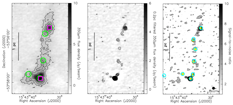
Figure 2: (left): 350$\mu m$ ArTéMiS image of part of SDC326.611+0.811 field (linear scale). Contours start at 1 Jy/beam by steps of 1 Jy/beam. The green circles show the positions of Herschel clumps from Elia et al. (2017), while the magenta squares show the positions of ATLASGAL clumps from Csengeri et al. (2014). (middle): Gaussian filtered image at 0.2 pc of the same source. Contours start at 0.5 Jy/beam in steps of 0.5 Jy/beam. (right): Signal-to-noise ratio map of the same source. Contours start at 2 by steps of 3. The yellow crosses show the position of the ArTéMiS sources, while the cyan circles show the positions of 70$\mu$m sources from Molinari et al. (2016).

2 Targets and observations

We targeted a total of 11 IRDCs from the Peretto & Fuller (2009) catalogue, selected to have a H₂ column density peak above $10^{23}$ cm^-2 and located at very similar distances, i.e. $2.6\pm 0.3$ kpc, with the exception of SDC326.796+0.386 (see Table 1). Kinematic distances to all sources, but one, have been estimated using the MALT90 N₂H⁺(1-0) data (Foster et al., 2013) and the Reid et al. (2009, 2014) galactic rotation model. Because SDC340.928-1.042 was not mapped by MALT90, we used the ThrUMMS ¹³CO(1-0) data instead (Barnes et al., 2015) to obtain its systemic velocity. These data show that it is part of the same molecular cloud as SDC340.969-1.020 and we therefore assigned the same velocity to both IRDCs. For all sources we adopted the near heliocentric distance as most IRDCs are located at the near distance (Ellsworth-Bowers et al., 2013; Giannetti et al., 2015). When more than one ArTéMiS clumps are part of a single IRDC we checked that the velocity and corresponding distances of individual clumps are similar, which turned to be always the case. The typical uncertainty on these distances is 15% (Reid et al., 2009). Table 1 shows the main properties of the sources, including their effective radii and background-subtracted masses as estimated from the Herschel column density maps from Peretto et al. (2016) within a H₂ column density contour level of $2\times 10^{22}$ cm^-2. The 11 IRDCs have been mapped as part of 5 individual fields which in some cases (in particular for the largest of all, i.e the SDC326 field) include extra sources. For all of these extra sources, we ensured that their kinematic distances were similar to the average field distance by using the same method as described above.

All targets were observed at 350$\mu$m with APEX and the ArTéMiS camera (Revéret et al., 2014; André et al., 2016) between September 2013 and August 2014 (Onsala projects O-091.F-9301A and O-093.F-9317A). The angular resolution at 350$\mu$m with APEX is $\theta_{\rm{beam}}=8^{\prime\prime}$. Observations have been carried out with individual maps of $6^{\prime}\times 6^{\prime}$, with a minimum of two coverages per field with different scanning angles. The scanning speed ranged from 20^′′/sec to $3^{\prime\prime}$/sec and the cross-scan step between consecutive scans from $6^{\prime\prime}$ to $12^{\prime\prime}$. The 350$\mu$m sky opacity (at zenith) and precipitable water vapour at the telescope were typically between 0.7 and 1.9 and between 0.35mm and 0.85mm, respectively. Absolute calibration was achieved by observing Mars as a primary calibrator, with a corresponding calibration uncertainty of $\sim$ 30%. Regular calibration and pointing checks were performed by taking short spiral scans toward the nearby secondary calibrators B13134, IRAS 16293, and G5.89 every $\sim$ 0.5-1.0 h. The pointing accuracy was within $\sim$ 3^′′. Data reduction was performed using the APIS pipeline running in IDL. The ArTéMiS images can be seen in Fig. 1 and in Appendix A.

3 Compact source identification

In order to identify compact sources in all our fields, we first convolved all ArTéMIS images with a Gaussian of FWHM of 0.2 pc ($\sim$ 15^′′ at 2.6 kpc), and subtracted that convolved image from the original image. By doing so, we filter our ArTéMiS images from emission on spatial scales $\geq 0.2$ pc, and the comparison between sources becomes independent of their background properties. We then identify compact sources using dendrograms (e.g. Rosolowsky et al., 2008; Peretto & Fuller, 2009) on signal-to-noise ratio (SNR) maps (see Fig. 2). For that purpose we computed noise maps, $\sigma_{map}$, from the ArTéMiS weight maps, $\omega_{map}$ (proportional to the integration time at every position in the map), and a noise calibration, $\sigma_{ref}$, estimated on an emission-free area of the filtered ArTéMiS maps following: $\sigma_{map}=\sigma_{ref}\sqrt{(\omega_{ref}/\omega_{map})}$, where $\omega_{ref}$ is the average weight estimated in the same region as $\sigma_{ref}$. The calibration $\sigma_{ref}$ is computed on the Gaussian filtered images (see Table 1 for median rms noise values). Our dendrogram source identification uses a starting level of $2\sigma_{map}$, a step of $3\sigma_{map}$ (i.e. all sources must have a minimum SNR peak of 5), and a minimum source solid angle of 50% of the beam solid angle which translates into a minimum effective diameter of $\sim$ 5.6^′′ ($\sim$ 0.07 pc at a distance of 2.6 kpc), i.e. 70% of the beam FWHM. The leaves of the dendrogram (i.e. structures that exhibit no further fragmentation within the boundaries set by the input parameters of the extraction) are then used as masks in the filtered ArTéMiS images to measure the peak flux density of every source. In the context of the present study, this is the only parameter we are interested in (see Sec. 5.2). As it can be seen in, e.g., Fig. 1, the noise in the image is non-uniform, and increases towards the edge of the image. In order to reduce the potential bias in the source detection created by a non-uniform noise, we defined, by hand and for each field, a mask that cuts out the noisy edges. In the following we only consider the sources that fall within this mask. In total, across all fields, we detect 203 compact ArTéMiS sources. Table 2 provides information on individual sources, and individual cutout images of each source can be found in Appendix C. Note that the source extraction parameters used in this paper are rather conservative and as a result faint sources might remain unidentified. However, the non-detection of such sources does not affect any of the results discussed here.

Table 2: Properties of the first 10 ArTéMiS sources identified in the SDC326 field. 1^st col.: source ID number; 2^nd col.: galactic longitude; 3^rd col.: galactic latitude; 4^th col: Original ArTéMiS peak flux density (i.e. non-filtered) and associated uncertainties; 5^th col.: Filtered ArTéMiS peak flux density and associated uncertainties; 6^th col.: Dust temperature estimated on 0.1pc scale (see Sec. 6.1) and associated uncertainties; 7^th col.: Gas mass estimated on 0.1pc scale (see Sec. 6.1) and associated uncertainties; 8^th: internal luminosity and associated uncertainties. If a value is given it means that the ArTéMiS source has a Herschel 70$\mu$m source from Molinari et al. (2016) associated to it; 9^th col.: Is there a Herschel clump from Elia et al. (2017) associated to it? ’y’ for yes, ’n’ for no; 10^th col.: Is there an ATLASGAL source from Csengeri et al. (2014) associated to it? ’y’ for yes, ’n’ for no; 11^th col.: Can we visually identify a mid-infrared (70$\mu$m and/or 8$\mu$m peak) peak on the individual cutout images in Appendix C? ’y’ for yes, ’n’ for no. The full table can be found online.

ID $\#$	$l$	$b$	$S_{\nu}^{\rm{pk}}$	$S_{\nu}^{\rm{pk}}$[filt]	Tdust[0.1pc]	Mgas[0.1pc]	Lint	H clump?	A clump?	mid-IR?
	(degree)	(degree)	(Jy/beam)	(Jy/beam)	(K)	(M⊙)	($\times 10^{3}$L⊙)
					SDC326	Field
1	326.7951	0.3817	$17.4\pm 5.2$	$9.8\pm 2.9$	$35.1\pm 7.0$	$3.8^{+2.9}_{-1.6}$	$1.05^{+0.26}_{-0.32}$	y	y	y
2	326.6328	0.5204	$3.9\pm 1.2$	$1.4\pm 0.4$	$30.3\pm 6.1$	$2.0^{+1.6}_{-0.9}$	$0.33^{+0.10}_{-0.10}$	y	n	y
3	326.6336	0.5288	$2.6\pm 0.8$	$1.0\pm 0.3$	$30.4\pm 6.1$	$1.4^{+1.1}_{-0.6}$	–	y	y	n
4	326.6577	0.5104	$6.7\pm 2.0$	$2.6\pm 0.8$	$30.7\pm 6.1$	$3.6^{+2.8}_{-1.6}$	$0.63^{+0.19}_{-0.19}$	y	n	y
5	326.6622	0.5200	$24.5\pm 7.4$	$11.6\pm 3.5$	$37.1\pm 7.4$	$11.0^{+8.3}_{-4.6}$	$9.41^{+2.64}_{-2.80}$	y	y	y
6	326.6584	0.5169	$13.8\pm 4.1$	$3.4\pm 1.0$	$25.1\pm 5.0$	$6.5^{+5.4}_{-3.0}$	–	y	y	n
7	326.6345	0.5328	$3.3\pm 1.0$	$1.6\pm 0.5$	$34.6\pm 6.9$	$1.7^{+1.4}_{-0.7}$	$0.87_{-0.26}^{+0.24}$	y	y	y
8	326.5636	0.5873	$2.5\pm 0.8$	$0.9\pm 0.3$	$22.4\pm 4.5$	$2.5^{+2.1}_{-1.2}$	–	n	n	y
9	326.6857	0.4950	$3.9\pm 1.2$	$1.9\pm 0.6$	$28.2\pm 5.6$	$3.0^{+2.8}_{-1.4}$	$0.21^{+0.07}_{-0.06}$	y	y	y
10	326.6272	0.5525	$1.9\pm 0.6$	$1.2\pm 0.4$	$35.0\pm 7.0$	$1.3^{+1.1}_{-0.6}$	$0.77^{+0.25}_{-0.23}$	y	n	y

Table 3: ArTéMiS source association statistics with Hi-GAL and ATLASGAL sources from Molinari et al. (2016), Elia et al. (2017), Csengeri et al. (2014) catalogues. Provides the number of ArTéMiS sources in each field, and how many are associated with at least one Hi-GAL clump, one Hi-GAL 70$\mu$m source, and one ATLASGAL source (see text). The last column provides the number of sources with no association from any of these three catalogues. The bottom line gives the summary across all fields.

Fields	$\#$ ArTéMiS	$\#$ ArTéMiS	$\#$ ArTéMiS	$\#$ ArTéMiS	$\#$ ArTéMiS
	sources	with Hi-GAL clumps	with Hi-GAL 70$\mu$m	with ATLASGAL	no association
SDC326	129	104	52	42	19
SDC328	31	24	13	9	5
SDC340	11	8	4	6	2
SDC343	13	12	11	9	1
SDC345	19	18	6	8	1
ALL	203	166	86	74	28

Table 4: Hi-GAL and ATLASGAL source association statistics (taken from Molinari et al. (2016), Elia et al. (2017), Csengeri et al. (2014) catalogues) with ArTéMiS sources. Provides the number of Hi-GAL clumps, Hi-GAL 70$\mu$m sources, and ATLASGAL sources in each field, and how many are associated with at least one ArTéMiS sources. The bottom line gives the summary across all fields.

Fields	$\#$ Hi-GAL clump	$\#$ Hi-GAL clumps	$\#$ Hi-GAL 70$\mu$m	$\#$ Hi-GAL 70$\mu$m	$\#$ ATLASGAL	$\#$ ATLASGAL
	in field	with ArTéMiS	in field	with ArTéMiS	in field	with ArTéMiS
SDC326	87	43	275	52	37	22
SDC328	20	13	114	13	14	8
SDC340	12	5	38	4	8	5
SDC343	12	8	35	11	9	8
SDC345	19	12	43	6	10	6
ALL	150	81	505	86	78	49

4 Associations of ArTéMiS sources with Hi-GAL and ATLASGAL source catalogues

In the past 10 years, far-IR and (sub-)millimetre continuum surveys of the Galactic plane have significantly contributed to improve our knowledge of massive star formation (Schuller et al., 2009; Molinari et al., 2010; Aguirre et al., 2011; Moore et al., 2015). However, even though these surveys have been, and still are, rich sources of information regarding massive star formation studies, one key issue is the lack of high-resolution, high-sensitivity observations of the cold dust on similar angular resolution as the Herschel 70$\mu$m band ($\sim 7^{\prime\prime}$ resolution) which traces the protostars’ luminosities. By filling in this gap, ArTéMiS observations allow us to unambiguously determine the envelope mass of young protostellar objects throughout the Galactic plane. In order to demonstrate the advancement that sensitive ArTésMiS observations provide over existing surveys, we here compare sub-millimetre source detections with Hi-GAL (Elia et al., 2017), and ATLASGAL (Csengeri et al., 2014), along with performing a Herschel 70$\mu$m source association using the Molinari et al. (2016) catalogue.

Association between our ArTéMiS sources and sources in published catalogues is performed by searching sources whose published coordinates lie within one beam of the central coordinates of the ArTéMiS source. We therefore used an angular separation of $8^{\prime\prime}$ when performing the 70$\mu$m association, $19^{\prime\prime}$ when performing the association with ATLASGAL sources, and $36^{\prime\prime}$ when performing the Hi-GAL clump association. The statistics of the number of sources within each field and their respective association with ArTéMiS sources are given in Table 3 and Table 4. These statistics show a number of important points. First, 14% of the ArTéMiS sources are newly identified sources that do not belong to any of the three catalogues we searched for. Also, about 54% of Hi-GAL clumps and 63% of ATLASGAL sources have an ArTéMiS detection associated to them. Finally, about 42% of the ArTéMiS sources have a published 70$\mu$m source associated to them, but when looking at the individual cutouts provided in Appendix C, one realises that an extra $\sim 25\%$ of sources have locally peaked 70$\mu$m or 8$\mu$m emission towards them. This means that about 67% of the ArTéMiS sources are protostellar, and about 33% are starless (down to the 70$\mu$m sensitivity of Hi-GAL of $\sim$ 0.1 Jy - Molinari et al., 2016).

Figure 3 shows examples for each association type (see also Appendix B and C). In this figure we display 7 sources, 4 of which are detected with ArTéMiS, 3 which are not. We also show these 7 sources at different wavelengths in order to better understand the type of sources that we do, and do not, detect with ArTéMiS. On the same figure, the symbols indicate when a source has been identified in the three different source catalogues used. By looking at Figure 3, it becomes clear that ArTéMiS is particularly good at identifying protostellar sources. In fact, even the source in the 4th column, which has not been identified in any of the three catalogue used, and which has therefore no Herschel 70$\mu$m entries in the Molinari et al. (2016) catalogue, seems to be associated with a faint point-like 70$\mu$m emission (as mentioned above, $\sim$ 25% of sources fall in this category of sources). On the other hand, all three sources displayed in Fig. 3 that have not been detected with ArTéMiS have no 70$\mu$m emission associated to them. The source in the 5th column is clearly seen in the ArTéMiS data, but falls just below our 5$\sigma$ threshold of detection. In a similar way as displayed in Fig. 3, we looked at all individual ArTéMiS sources we identified to ensure the quality of the detection. Individual images of each ArTéMiS source can be found in Appendix C.

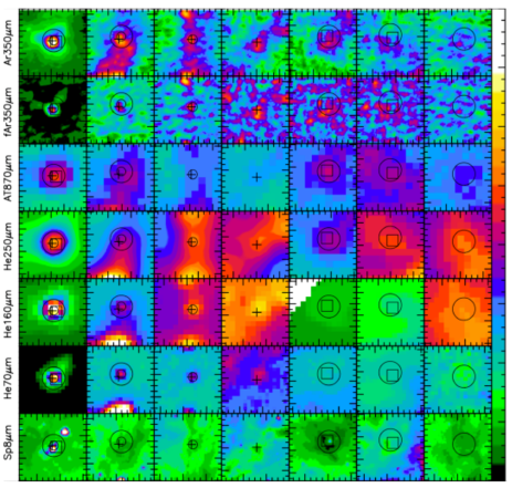
Figure 3: Examples of association types. Each column represent a different source, the first four being ArTéMiS detections (from left to right: SDC326 #123, #126, #127, #118), the last 3 being Herschel and/or ATLASGAL detections. Each row represents a given wavelength, from top to bottom: ArTéMiS 350$\mu$m; Filtered ArTéMiS 350$\mu$m; ATLASGAL 870$\mu$m; Herschel 250$\mu$m; Herschel 160$\mu$m; Herschel 70$\mu$m; Spitzer 8$\mu$m. The different symbols indicate if the source appear in a given catalogue: Crosses for ArTéMiS detections; Large circles for Herschel clumps; Small circles for Herschel 70$\mu$m detections; Squares for ATLASGAL detections.

5 Physical properties of ArTéMiS sources

5.1 Dust temperatures

A key characteristic of the compact sources we identified within our ArTéMiS data is their dust temperature. Dust temperatures are needed to estimate the mass of these sources, but also can be used as an evolutionary tracer of the sources as dust tends to become warmer as star formation proceeds. We have here computed dust temperatures in two different ways.

5.1.1 Far-infrared colour temperature, T_col

In order to compute dust temperatures of interstellar structures one usually needs multi-wavelength observations to get a reasonable coverage of the spectral energy distribution. One problem we are facing is the lack of complementary far-IR sub-millimetre observations at similar angular resolution to our ArTéMiS data. Herschel observations represent the best dataset available regarding the characterisation of cold interstellar dust emission. However, at 250$\micron$, the angular resolution of Herschel is $\sim 2.5$ times worse than that of APEX at 350$\micron$. Another big difference between the two datasets is that Herschel is sensitive to all spatial scales, and therefore recovers a lot more diffuse structures than within our ArTéMiS data. Here, we use the ratio between the 160$\mu$m and 250$\mu$m Herschel intensities at the location of each ArTéMiS source as a measure of the source dust temperature (Peretto et al., 2016). In that respect, we first need to measure the local background intensities of each source. We do this by measuring the minimum 250$\mu$m intensity value within an annulus surrounding each of the ArTéMiS source, along with the corresponding 160$\mu$m intensity at the same position. The reason behind choosing the lowest 250$\mu$m intensity is that the local background around these sources can be complex, and made of other compact sources, filaments, etc… Therefore, taking, as it is often done, an average of the intensities within the annulus would result in an uncertain background intensity estimate. By focussing on the single faintest 250$\mu$m pixel, we are relatively confident to take the background at the lowest column density point within the annulus, which should provide a reasonable estimate of the local background of the compact sources we are interested in. We finally subtract the local background measurements from the measured 250$\mu$m and 160$\mu$m peak intensities within the source mask. The resulting background-subtracted fluxes are used to compute the far-infrared colour dust temperatures of each ArTéMiS sources (Peretto et al., 2016).

5.1.2 Internal temperature, T_int

For a spherical protostellar core, in the situation where dust emission is optically thin, and where the bulk of the source luminosity is in the far-infrared, one can show that flux conservation leads to the following temperature profile (Terebey et al., 1993):

$$T_{\rm{int}}=T_{0}\left(\frac{r}{r_{0}}\right)^{-2/(\beta+4)}\left(\frac{L_{\rm{int}}}{L_{0}}\right)^{1/(\beta+4)}$$ (1)

where $\beta$ is the spectral index of the specific dust opacity law, and ($T_{0},r_{0},L_{0}$) are normalisation constants and, following Terebey et al. (1993), are here set to (25 K, 0.032 pc, 520 $L_{\odot}$), respectively. By integrating over the volume of the core, and assuming a given volume density profile, one can then obtain an expression for the mass-averaged temperature $\overline{T}_{\rm{int}}$. Here, we assume that $\rho\propto r^{-2}$, which leads to the following relation:

$$\overline{T}_{\rm{int}}=\left(\frac{\beta+4}{\beta+2}\right)T_{\rm{int}}$$ (2)

Given the luminosity of the source one can then compute the average dust temperature within a given radius $r$. In order to compute the bolometric luminosities of ArTéMiS sources we exploit their tight relationship with 70$\mu$m fluxes (Dunham et al., 2008; Ragan et al., 2012; Elia et al., 2017). Here, each ArTéMiS source has been checked against the Molinari et al. (2016) 70$\mu$m source catalogue (see Sec. 4) and their corresponding 70$\mu$m fluxes come from the same catalogue. Then, we convert fluxes into luminosities using the following relation (Elia et al., 2017):

$$L_{\rm{int}}=25.6\,\left(\frac{F_{70\mu m}}{10\rm{Jy}}\right)\left(\frac{d}{1\rm{kpc}}\right)^{2}L_{\odot}$$ (3)

where $F_{70\mu m}$ is the 70$\mu$m flux of the ArTéMiS source in Jy. This relation is very similar to that obtained for low-mass protostellar objects by Dunham et al. (2008):

$$L_{\rm{int}}=20.0\,\left(\frac{F_{70\mu m}}{10\rm{Jy}}\right)^{0.94}\left(\frac{d}{1\rm{kpc}}\right)^{1.88}L_{\odot}$$ (4)

Since we are using the same Herschel datasets as in Elia et al. (2017), we here use the former relationship. Note that these authors have identified a third relation between $L_{\rm{int}}$ and $F_{70\mu m}$ for sources that do not have a known Spitzer or WISE mid-infrared at 24$\mu$m or 21$\mu$m respectively. However, for simplicity we here only use Eq. (3), the dependence of $T_{\rm{int}}$ on $L_{\rm{int}}$ is in any case very shallow. Finally, by plugging in the corresponding luminosities in equation (1), and by setting $\beta=2$ (e.g. Hildebrand 1983), we can obtain $\overline{T}_{\rm{int}}$ for every ArTéMiS protostellar source.

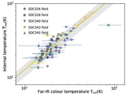
Figure 4: Far-infrared colour temperature obtained from the ratio of the Herschel 160$\mu$m to 250$\mu$m fluxes, versus the internal temperature obtained from the Herschel 70$\mu$m flux for each protostellar ArTéMiS source. The solid yellow line represents the median value of the $\overline{T}_{\rm{int}}/T_{col}$ ratio. The grey shaded area shows the 16^th to 84^th percentile range.

5.1.3 Comparison between T_col and $\overline{T}_{\rm{int}}$

Our estimates of T_col and $\overline{T}_{\rm{int}}$ use independent Herschel data, and make use of different sets of assumptions to compute the same quantity, i.e the dust temperature of ArTéMiS sources. In order to decide which of these two sets of temperatures is the most appropriate to use, we plotted them against each other (see Fig. 4). This can only be done for ArTéMiS sources with an associated 70$\mu$m source. For the purpose of making Fig. 4, $\overline{T}_{\rm{int}}$ has been here estimated within a radius equivalent to the Herschel 250$\mu$m beam (i.e. 0.23pc at 2.6 kpc distance) so that the comparison remains valid. Uncertainties have been estimated by using Monte Carlo propagation. Uncertainties for $\overline{T}_{\rm{int}}$ are much lower as a result of its shallow dependency on $F_{70\mu m}$. One can see that the two sets of values are well correlated to each other, with a median ratio $\overline{T}_{\rm{int}}/T_{\rm{col}}=1.28^{+0.20}_{-0.25}$. This shows that, for most of the points in Fig. 4, the far-IR colour temperature is lower by $\sim 28\%$ compared to its internal temperature counterpart. Interestingly, Peretto et al. (2016) showed that far-IR colour temperature were also lower by $\sim 20\%$ on average compared to dust temperatures estimated from a 4-point spectral energy distribution fit of the Herschel data. It is also worth noting that $\overline{T}_{\rm{int}}$ provides an upper limit to the temperature of compact sources as its calculation assumes optically thin emission and a spherically symmetric density profile that peaks at the location of the 70$\mu$m bright protostar. Deviations from these assumptions would lead to lower mass-averaged temperatures. As a consequence, in the remaining of the analysis, the quoted temperatures are computed using:

$$T_{\rm{dust}}=1.2(\pm 0.2)\,T_{\rm{col}}$$ (5)

with the exception of the sources that have $T_{col}>\overline{T}_{\rm{int}}$, for which we used $\overline{T}_{\rm{int}}$. Using Eq. (5) allows us to compute dust temperatures consistently for all ArTéMiS sources, something that the use of $\overline{T}_{\rm{int}}$ would not allow us to do as it requires the detection of a 70 $\mu$m source. Finally, note that these temperatures are estimated on the scale of the Herschel 250$\mu$m beam, i.e. 0.23 pc at 2.6 kpc distance, which is slightly more than twice larger than the ArTéMiS beam itself. According to Eq. (1), this can lead to a systematic underestimate of dust temperatures of $\sim$ 30% for protostellar sources. The impact of this important systematic uncertainty on temperature is discussed in Section 6.

5.2 Masses

The mass of each ArTéMiS source is estimated assuming optically thin dust emission, uniform dust properties (temperature and dust emissivity) along the line of sight, and uniform dust-to-gas mass ratio. With these assumptions, the source mass is given by:

$$M_{\rm{gas}}=\frac{d^{2}F_{\nu}}{R_{d2g}\kappa_{\nu}B_{\nu}(T_{d})}$$ (6)

where $d$ is the distance to the source, $F_{\nu}$ is the source flux, $R_{d2g}$ is the dust-to-gas mass ratio, $\kappa_{\nu}$ is the specific dust opacity at frequency $\nu$, and $B_{\nu}(T_{d})$ is the Planck function at the same frequency and dust temperature $T_{d}$. Here, we used $R_{d2g}=0.01$ and $\kappa_{\lambda}=4.44\left(\frac{\lambda}{450\rm{\mu m}}\right)^{-2}$ cm²/g (e.g. Hildebrand, 1983; Könyves et al., 2015). Regarding distances, for each field we used the average distance of the individual clumps lying within them, with the exception of SDC326.796+0.386 which has been excluded from the rest of this study since it is much closer than all the other sources (see Table 1). Finally, regarding the dust temperature we use $T_{\rm{dust}}$ as defined in Sec. 5.1.3. As far as uncertainties are concerned, we used 30%, 15%, and 20% uncertainty for $F_{\nu}$, $d$, and $T_{\rm{dust}}$, respectively, that we propagated in Eq. (6) using Monte Carlo uncertainty propagation.

The dendrogram analysis done here provides boundaries for every leaf identified in the ArTéMiS images. While we can use these to define the physical boundaries of compact sources, it is not clear if such an approach is the best. First, in some cases, especially for starless sources, these boundaries seem to encompass sub-structures that just fail to pass the detection criterion (i.e. local minimum to local maximum amplitude larger than 3$\sigma_{map}$). Also, nearly all high angular resolution ($\leq 1^{\prime\prime}$) observations of similar sources show sub-fragmentation (e.g. Svoboda et al., 2019; Sanhueza et al., 2019; Louvet et al., 2019) casting doubts on the true physical meaning of the identified ArTéMiS compact sources. Our approach here is more generic: we compute the mass within the ArTéMiS beam solid angle at the location of the peak flux density of every identified leaf. Because the sources analysed here are all within a very narrow range of distances (see Table 1), the proposed approach provides a measure of compact source masses within a comparable physical diameter of $\sim$ 0.10$\pm 0.01$ pc.

6 The mass-temperature-luminosity diagram

6.1 The ArTéMiS view

As protostars evolve with time, the temperature, luminosity, and mass of their envelopes change. The accretion history of these protostellar envelopes will define what their tracks will be on a mass vs. dust temperature diagram. Large statistical samples of protostellar sources within star-forming regions can therefore help constraining the accretion histories of these objects. In Figure 5 we show the mass vs. dust temperature diagram for all identified ArTéMiS sources with masses estimated using the temperatures given by Eq. (5) and the ArTéMiS peak flux density. On the same figure we have added the mass sensitivity limits for the minimum and maximum distances of our sample. One advantage of a mass vs. dust temperature diagrams over a more standard mass vs. luminosity one is that all sources, starless and protostellar, can easily be represented on it.

Figure  5 displays a couple of important features. First, we notice the presence of warm ($T_{\rm{dust}}>30$ K) starless sources, which might seem surprising at first. However, these sources are all located in very specific environments, that is in the direct vicinity of some of the more luminous young stellar objects we have mapped. For instance, starless sources #14, 17, 18, and 20 in the SDC328 field have all dust temperatures larger than 30K (including the two warmest ones displayed on Fig. 5 at 44K and 55K) and are all located within a radius of 0.6 pc of sources #13 and #19. These two sources have internal luminosities of $\sim 8,500$ L_⊙ and $\sim 55,000$ L_⊙, respectively. According to Eq.(1), sources with such luminosities can warm up dust up to 30K within a radius of 0.3 pc and 0.6 pc. It is therefore unsurprising to find starless sources with temperatures in excess of 30K. However, it is unclear if such sources are gravitationally bound and will form stars in the future. As a reference, a Bonnor-Ebert sphere of 0.05 pc radius and 40 K gas temperature has a critical mass of $\sim 4$ M_⊙ (Bonnor, 1956; Ebert, 1955). In Fig. 5 we added, as a blue-dotted line, the critical half-mass Bonnor-Ebert relationship for a core radius of 0.05 pc, $\frac{1}{2}M_{\rm{BE}}^{\rm{crit}}=1\times\left(\frac{T}{20K}\right)$ M_⊙. Starless sources below that line are very likely to be unbound structures.

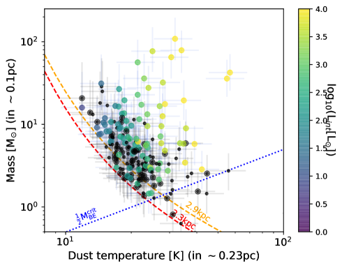
Figure 5: Mass versus dust temperature for all ArTéMiS sources. The temperatures are here estimated on the Herschel 250$\mu$m beam size (i.e. 0.23pc), while the ArTéMiS flux used to compute the mass is estimated on the ArTéMiS beam size (i.e. 0.1pc). The symbols are coded by the sources’ internal luminosities. Sources with no 70$\mu$m association from the Molinari et al. (2016) catalogue are represented as black symbols. Amongst these, those that do not display any local 70$\mu$m or 8$\mu$m peaks on the individual images presented in Appendix C are represented as filled circles. Those that do present a visually-identified mid-infrared peak in these individual images have in addition a larger empty circular symbol. The dashed lines show the mass sensitivity limits at the two extreme distances of the sources in our sample. The blue dotted line gives half the thermal critical Bonnor Ebert mass for a core radius of 0.05 pc as a function of temperature.

An even more important feature of Fig. 5 is the presence of massive protostellar sources with masses beyond 30 M_⊙ and the absence of equally massive starless counterparts. This is in line with the early result by Motte et al. (2007) on the lack of massive pre-stellar cores in Cygnus. We also note that a luminosity gradient seems to run from the low-mass low-temperature corner to the high-mass high-temperature one. These trends, however, are very much subject to the relative temperature difference between starless and protostellar sources. As noted in Sec. 5.1.3, the flux and temperature measurements used to build Fig. 5 are inconsistent with each other since they are estimated on different spatial scales, i.e. 0.1 pc and 0.23 pc, respectively. Because the temperature profiles of starless and protostellar sources scales are different, this inconsistency could create artificial trends in a diagram such as that of Fig. 5. We attempt to correct for it using Eq. (1) for protostellar sources, and assuming that starless sources are isothermal. The mass-averaged temperature correction factor for protostellar sources is given by $(0.23/0.1)^{1/3}=1.32$ (from Eq. (1), with $\beta=2$). The temperature of starless sources are left unchanged. The resulting corrected temperature vs mass diagram is shown in Fig. 6. On this figure, we see that the trends observed in Fig. 5 (i.e. protostellar sources being more massive than starless ones, and the presence of a diagonal luminosity gradient) are mostly still present, albeit with slightly decreased significance. All data (temperature, mass, and luminosity) used to produce that figure is provided in Table 1.

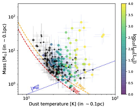
Figure 6: Same as Fig. 5 but temperatures and masses have been rescaled to a common spatial scale of 0.1pc.

The correction we made on the source temperatures relies on the fact that our starless/protostellar classification is robust. However, as mentioned in Sec. 4, $\sim 43\%$ of the ArTéMiS sources that do not have a 70$\mu$m association from the Molinari et al. (2016) catalogue seem to have a 70$\mu$m and/or 8$\mu$m emission peak when looking at the individual source images provided in Appendix C (in Figs. 5 and 6 these sources are marked as black empty circular symbols with a smaller black filled symbol in them). Also, when observed with ALMA at high angular resolution, single-dish starless sources observed in high-mass star-forming regions systematically fragment into a set of low-mass protostellar cores (e.g. Svoboda et al., 2019). This shows that the classification of sources as starless based on single-dish continuum observations (e.g. with Herschel) should be viewed with caution in these regions. The net impact of wrongly classifying a protostellar source as starless would be to underestimate its temperature and therefore overestimate its mass. In other words, the trends mentioned earlier can only be strengthened by correcting for such misclassifications. This is particularly true if the handful of cold massive sources above 10 $M_{\odot}$ would turn out to be protostellar (as Fig. 6 shows it is likely to be the case for at least three of these sources).

Finally, we also note that the relationship provided by Eq. (5), even though established on protostellar sources only, has been applied to all sources, including starless ones. This seems to be the most appropriate approach since the ratio $\overline{T}_{\rm{int}}$ over $T_{\rm{col}}$ does not appear to be a function of the internal luminosity (see Fig. 4). However, for completeness, we do show in Appendix D a version of the mass versus temperature diagram in which we used $T_{\rm{dust}}=T_{\rm{col}}$ for the starless sources while applying the same correction factors for the protosellar sources.

Given the relatively low number of sources in our sample, the trends mentioned above are rather speculative. Nevertheless, it remains interesting to determine whether or not one can recover these trends with simple models that mimic both core-fed and clump-fed accretion scenarios.

6.2 Accretion models

Following Bontemps et al. (1996), André et al. (2008), and Duarte-Cabral et al. (2013), we built a simple accretion model that is aimed at reproducing the evolution of a protostellar core as the central protostar grows in mass. The set of equations that describes the mass growth of a protostar, and the parallel mass evolution of the core, is:

$$\frac{dm_{*}}{dt}=\dot{m}_{*}$$ (7)

$$\frac{dm_{\rm{core}}}{dt}=-\dot{m}_{*}+\dot{m}_{\rm{clump}}$$ (8)

$$\dot{m}_{*}=\epsilon_{cs}\frac{m_{\rm{core}}}{\tau_{\rm{core}}}$$ (9)

$$\dot{m}_{\rm{clump}}=\epsilon_{cc}\frac{m_{\rm{clump}}}{\tau_{\rm{clump}}}$$ (10)

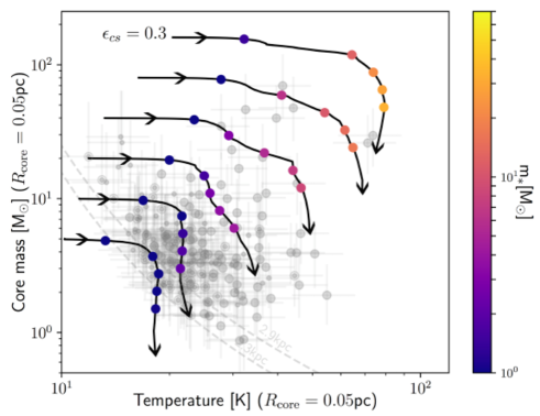
Figure 7: Core-fed models. Each track has been computed for a different initial core mass, from bottom to top ${m}_{\rm{core}}(t=0)=[5,10,20,40,80,160]$ M_⊙. The coloured symbols represent the position of the cores at times $t=[9\times 10^{3},9\times 10^{4},1.8\times 10^{5},2.7\times 10^{5},3.6\times 10^{5}]$ yr. The colour codes the stellar mass at these times as displayed by the colour bar. The background grey symbols are those presented in Fig. 6. Note that sources with $M_{\rm{gas}}<\frac{1}{2}M_{\rm{BE}}^{\rm{crit}}$ have been removed.

where $m_{*}$ is the mass of the protostar, $m_{\rm{core}}$ is the mass of the core, $\dot{m}_{*}$ is the mass accretion rate of the protostar, $\dot{m}_{\rm{clump}}$ is the mass accretion rate of the core from the clump, $\tau_{\rm{core}}$ is the characteristic star formation timescale on core scale, $\tau_{\rm{clump}}$ is the characteristic star formation timescale on clump scale, $\epsilon_{cs}$ is the star formation efficiency from core to star (the fraction of the core mass that is being accreted onto the protostar), and finally $\epsilon_{cc}$ is the core formation efficiency from clump to core (the fraction of the clump mass that ends up in a core). In the context of this set of equations, core-fed scenarios differentiate themselves from clump-fed ones by having $\dot{m}_{\rm{clump}}=0$. This is the framework Duarte-Cabral et al. (2013) worked in. The clump-fed models, on the other hand, are presented here for the first time. In the following, we explore both type of scenarios.

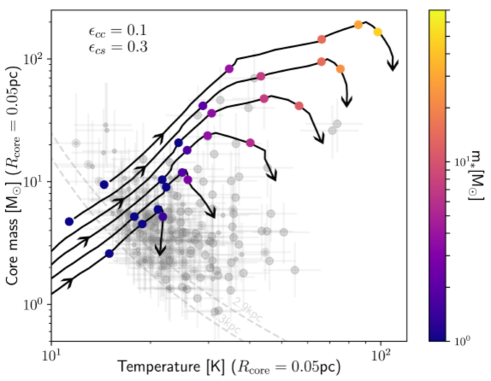
Figure 8: Clump-fed models. Each track has been computed for a different clump mass, from bottom to top $m_{\rm{clump}}=[100,200,400,800,1600,3200]$ M_⊙.The coloured symbols represent the position of the cores at times $t=[3\times 10^{4},3\times 10^{5},6\times 10^{5},9\times 10^{5},1.2\times 10^{6}]$ yr. The colour codes the stellar mass at these times as displayed by the colour bar. The background grey symbols are those presented in Fig. 6. Note that sources with $M_{\rm{gas}}<\frac{1}{2}M_{\rm{BE}}^{\rm{crit}}$ have been removed.

Equations 7 to 10 provide a description of the mass evolution of both the protostar and the surrounding core. However, in order to produce a mass vs temperature diagram one needs to compute, in parallel to the mass evolution, the evolution of the luminosity of the system. To do this, we used the protostellar evolutionary tracks from Hosokawa & Omukai (2009). These are well adapted to the formation of massive stars. These tracks provide, for a given mass accretion rate and given protostar mass, the total luminosity of the system that includes both accretion luminosity and stellar luminosity. At each time step of our numerical integration of Eq. (7) to (10), we linearly interpolate the luminosity between the closest tracks. Finally, using Equations (1), (2) and (5) one can then compute the theoretical equivalent of Fig. 6.

In the context of core-fed scenarios, cores refer to the fixed-mass reservoir of individual protostars. In nearby low-mass star-forming regions these cores have typical sizes ranging from 0.01pc to 0.1pc (e.g. Könyves et al., 2015, 2020). These can be understood as the typical sizes of the gravitational potential well’s local minima, decoupled from their larger-scale surroundings. In the context of clump-fed scenarios, these cores are located within a larger-scale minimum defined by the presence of a surrounding parsec-scale clump that continuously feeds the cores with more mass. While Eqs (7) to (10) do not explicitly refer to any size-scale, the calculation of the mass-averaged temperature, Eq. (1), does require setting a characteristic core scale. Here, we are limited by the spatial resolution of the ArTéMiS observations, i.e. $\sim 0.1$ pc at the distance of the observed regions. Hence, in the following models, we use $R_{\rm{core}}=0.05$ pc.

Figure 7 shows a set of models with $\dot{m}_{\rm{clump}}=0$ (effectively core-fed models), and for 6 different initial (prestellar) core masses, ${m}_{\rm{core}}(t=0)=[5,10,20,40,80,160]$ M_⊙, all with a radius $R_{\rm{core}}=0.05$ pc. As suggested by Duarte-Cabral et al. (2013) we set $\tau_{\rm{core}}=3\times 10^{5}$ yr for all sources. Note that the exact value used for this timescale does not change the shape of the modelled tracks, a shorter timescale would only make the evolution faster. We also set $\epsilon_{\rm{cs}}=0.3$, lower than the value of 0.5 used in Duarte-Cabral et al. (2013) to represent the fact that the modelled cores are larger. In essence, the tracks presented in Fig. 7 are identical to those presented in Fig. 5 of Duarte-Cabral et al. (2013) (albeit the slightly different set of parameter values). While these models cover a similar range of mass and temperature as the ArTéMiS sources, they require the existence of massive prestellar cores that should reside in the top left corner of the plot. For the tracks describing the evolution of the most massive stars (${m}_{\rm{core}}(t=0)=[80,160]$ M_⊙), such starless sources are not present in our ArTéMiS sample. But one could argue though that such core-fed models provide a good description of the data for initial core masses $m_{\rm{core}}\leq 30$ M_⊙ which, according to the models, would form stars with $m_{*}\leq 9$ $M_{\odot}$. These same intermediate-mass tracks also explain the presence of luminous objects (i.e. $L_{\rm{int}}\geq 10^{3}$ L_⊙) with low associated core masses as sources that arrive at the end of their accretion phase.

Figure 8 shows a set of tracks with $\dot{m}_{\rm{clump}}\neq 0$ (effectively clump-fed models) and ${m}_{\rm{clump}}$=[100, 200, 400, 800, 1600, 3200] M_⊙. They all start with the same initial core mass $m_{\rm{core}}(t=0)$=1 M_⊙, the typical Jeans mass in dense molecular clumps. We also set $\epsilon_{cc}=0.1$, $\epsilon_{\rm{cs}}=0.3$, and $\tau_{\rm{clump}}=\tau_{\rm{core}}=1\times 10^{6}$ yr, i.e. the clump crossing time controls the infall. This assumption remains valid as long as the time to regenerate the mass of the core, i.e. $\frac{m_{\rm{core}}}{m_{\rm{clump}}}\tau_{\rm{clump}}$, is shorter than the core freefall time. This is verified at all times in the models. We set a longer timescale for clump-fed models than for core-fed models since the gas density of clumps is necessarily lower than that of the cores embedded within them. However, as for the core-fed models, the exact value used for the timescale in the clump-fed models does not change the shape of the tracks. Finally, the core accretion phase is stopped once $t>\tau_{\rm{clump}}$. Note that the point of this paper is not to proceed to a thorough examination of the parameter space of the proposed model but rather to evaluate if such models could generate a reasonable agreement with the observations. As we can see in Fig. 8, these models do also cover a similar range in mass and temperature as the observations, and are able to explain the formation of the most massive stars without the need for massive starless sources. In addition, the modelled tracks evolved along the evolutionary gradients that we tentatively see in the observations. These models are therefore rather promising in the context of trying to pinpoint the physical mechanisms lying behind the mass accretion history of the most massive stars.

One could argue that the spatial resolution of the ArTéMiS data presented here (i.e. 0.1pc) is not enough to probe individual pre/protostellar cores, and that the ArTéMiS sources are therefore likely to be sub-fragmented. While this might be true, it is also likely that the measured ArTéMiS flux of each source is dominated by the brightest unresolved core lying within the ArTéMiS beam. In fact, there is evidence that this is indeed the case as Csengeri et al. (2017) observed 8 of the most massive ArTéMiS sources presented here with ALMA at $\sim 3^{\prime\prime}$ resolution, nearly 3 times better resolution than ArTéMiS and corresponding to a size scale of $\sim 8000$ AU. On that scale, the fraction of the ALMA flux locked in the brightest ALMA compact source is between 50% to 90% of the total flux. Also, Csengeri et al. (2018) presented ALMA observations of source SDC328#19 (one of the two warmest sources presented in, e.g., Fig. 5, at an angular resolution of 0.17^′′ (i.e. $\sim 500$AU at 2.75 kpc). There, no sub-fragmentation is observed.

A comparison between our ArTéMiS observations and models on scales smaller than the ArTéMiS beam requires a set of extra assumptions and is therefore most uncertain. Such comparison is provided in Appendix E.

7 Conclusions

The key observational constraint regarding core-fed star formation is the existence of massive prestellar cores. The most massive starless sources identified here have masses of $\sim 30$ M_⊙ in a 0.1pc source size, which is 3 to 4 times less massive that the most massive protostellar sources identified in the observed fields (within the same size). Taken at face value, this would suggest that the most massive ArTéMiS sources we identified keep growing in mass while simultaneously feeding massive protostar(s) at their centre, and that clump-fed models describe best the formation of massive stars. Our data though does not exclude the possibility of core-fed star formation for intermediate-mass stars. Therefore, a transition regime could exist between core-fed and clump-fed star formation scenarios around $m_{*}=8$ M_⊙.

Most of the ArTéMiS sources studied here are likely to be sub-fragmented into a number of unresolved individual cores. A larger fragmentation level in our ArTéMiS protostellar sources, compared to the starless ones, could invalidate our former conclusion and instead favour core-fed scenarios. High-angular resolution observations on 1000 AU scale of massive 0.1pc-size sources, both starless and protostellar, have indeed revealed sub-fragmentation (e.g. Bontemps et al., 2010; Palau et al., 2013; Svoboda et al., 2019; Sanhueza et al., 2019). There is however no evidence that starless sources are less fragmented than protostellar ones, and if anything, these studies show the opposite. We already know that for 8 of the most massive sources from our sample, ALMA observations at $\sim 8000$ AU resolution reveal that most of the ALMA flux comes from the brightest core (Csengeri et al., 2017), and for the one source observed at $\sim 500$ AU resolution, a single core is identified(Csengeri et al., 2018). It is therefore likely that our conclusions remain valid even on small scales (see also Appendix E).

Another argument that seems to favour the clump-fed scenario is the the shape of the upper envelope of the data point distribution in Fig. 5. As it can be seen in Fig. 8, this envelope is naturally reproduced by clump-fed tracks. Ideally, we would like to generate modelled density plots of such diagrams and compare to its observed equivalent. However, the number of sources at our disposition is currently too small to perform such an analysis. Larger number statistics would also allow us to set stronger constraints on the existence of starless sources with masses above 30 M_⊙ and their statistical lifetimes. By mapping all observable massive star-forming regions within a 3 kpc distance radius from the Sun, the CAFFEINE large programme on APEX with ArTéMiS aims at providing enough source statistics to build temperature vs mass density plots, allowing us to definitely conclude on the dominant scenario regulating the formation of massive stars and on the existence of a transition regime between core-fed and clump-fed star formation.

Appendix A ArTéMiS images

In this Appendix we present the ArTéMiS images for the SDC328, SDC340, SDC343, and SDC345 fields.

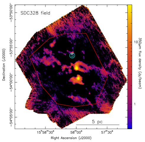
Figure 9: Same as Fig. 1 for the SDC328 field

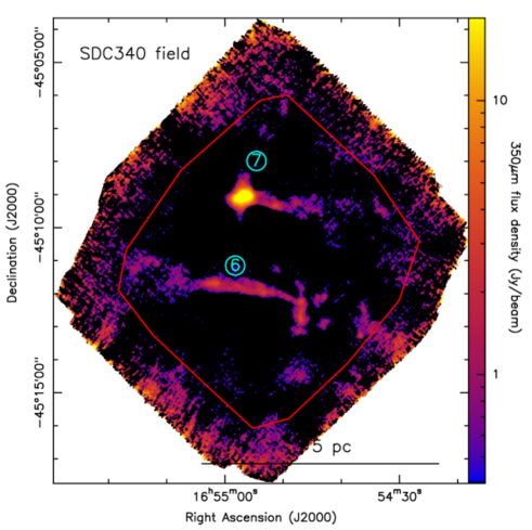
Figure 10: Same as Fig. 1 for the SDC340 field

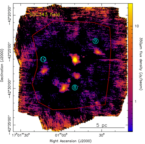
Figure 11: Same as Fig. 1 for the SDC343 field

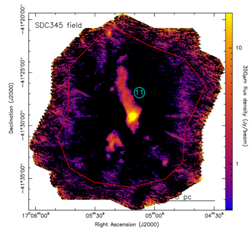
Figure 12: Same as Fig. 1 for the SDC345 field

Appendix B Images of ArTéMiS sources associations

In this Appendix we present the ArTéMiS images with the locations of the Herschel 70$\mu$m sources (Molinari et al., 2016), Herschel clumps (Elia et al., 2017), and ATLASGAL clumps (Csengeri et al., 2014) for the SDC326, SDC328, SDC340, SDC343, and SDC345 fields.

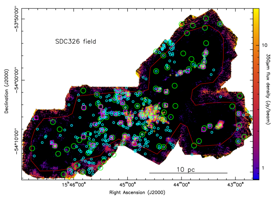
Figure 13: Background image is the same as in Fig. 1. The yellow crosses mark the central positions of the identified ArTéMiS sources. The cyan circles mark the central positions of the Hi-GAL 70$\mu$m sources (Molinari et al. 2016). The green circles mark the central positions of the Herschel clumps (Elia et al. 2017). The purple squares mark the central positions of the ATLASGAL sources (Csengeri et al. 2014). The red solid line shows the area over which all source statistics presented in the paper have been calculated (i.e. excluding the noisy edges of the ArTéMis image).

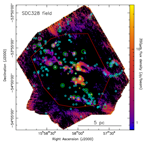
Figure 14: Same as Fig. 13 for the SDC328 field

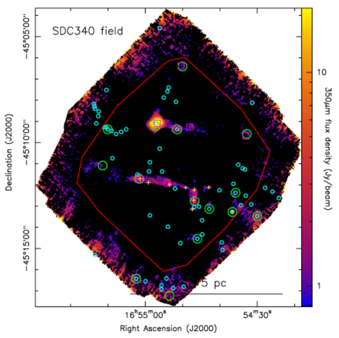
Figure 15: Same as Fig. 13 for the SDC340 field

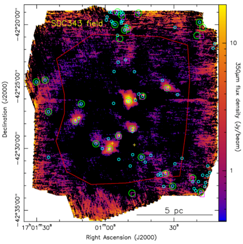
Figure 16: Same as Fig. 13 for the SDC343 field

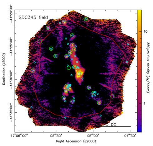
Figure 17: Same as Fig. 13 for the SDC345 field

Appendix C Individual cutout images around each robust ArTéMiS source

In this Appendix we present individual cutout images of each ArTéMiS source (see Sec. 3).

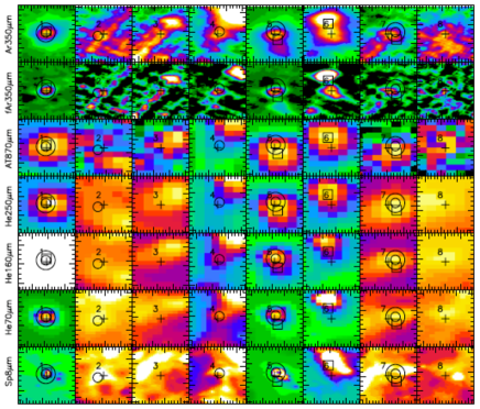
Figure 18: Cutout images of each individual ArTéMiS sources identified in the SDC326 field. Each cutout is a 1arcmin by 1arcmin box centred on the source position. Each column corresponds to a different source, the id number of source is indicated in each panel. Each row corresponds to a different wavelength or image type. The 1st row presents the original ArTéMiS image of the source; the 2nd row to the filtered ArTéMiS image; the 3rd to ATLASGAL; the 4th to Herschel 250$\mu$m; the 5th to Herschel 160$\mu$m;the 6th toHerschel 70$\mu$m; the 7th to Spitzer 8$\mu$m. The central black crosses mark the central position of the ArTéMiS source. The black squares mark the position of ATLASGAL sources (Csengeri et al., 2014). The small black circles mark the positions of Herschel 70$\mu$m sources (Molinari et al., 2016). The large black circles mark the positions of Herschel clumps (Elia et al., 2017)

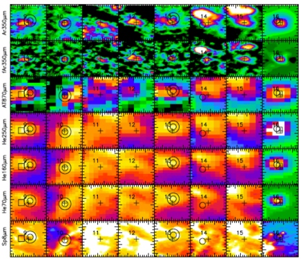
Figure 19: Figure C1 continued.

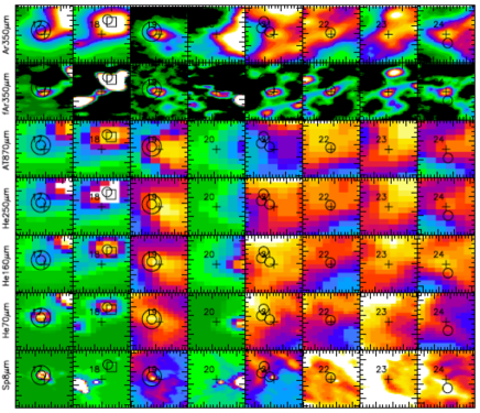
Figure 20: Figure C1 continued.

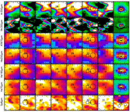
Figure 21: Figure C1 continued.

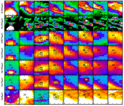
Figure 22: Figure C1 continued.

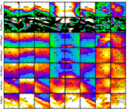
Figure 23: Figure C1 continued.

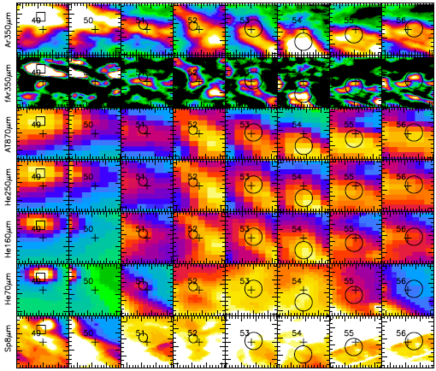
Figure 24: Figure C1 continued.

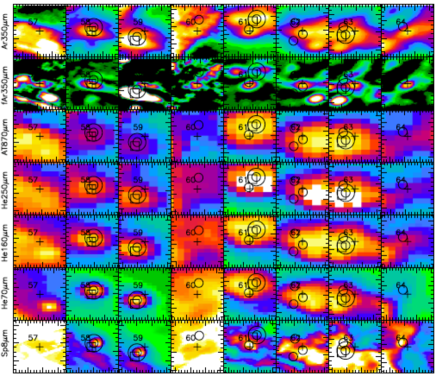
Figure 25: Figure C1 continued.

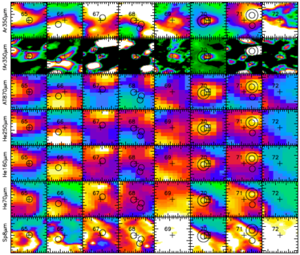
Figure 26: Figure C1 continued.

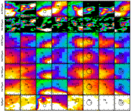
Figure 27: Figure C1 continued.

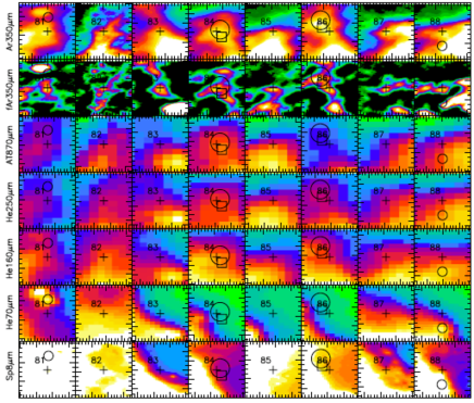
Figure 28: Figure C1 continued.

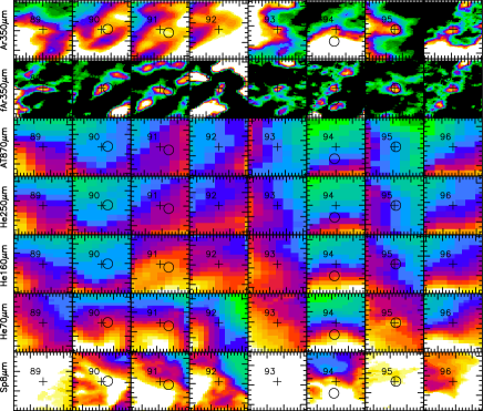
Figure 29: Figure C1 continued.

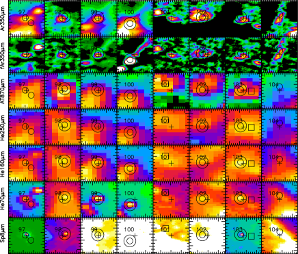
Figure 30: Figure C1 continued.

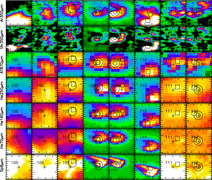
Figure 31: Figure C1 continued.

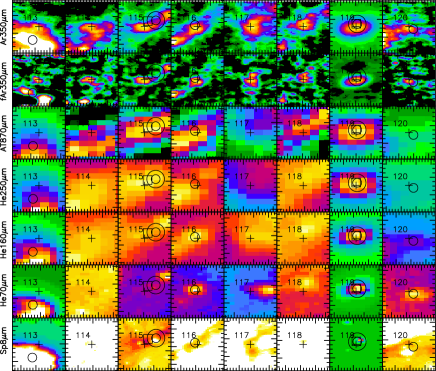
Figure 32: Figure C1 continued.

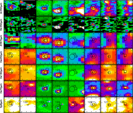
Figure 33: Figure C1 continued.

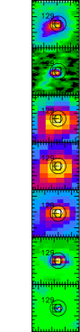
Figure 34: Figure C1 continued.

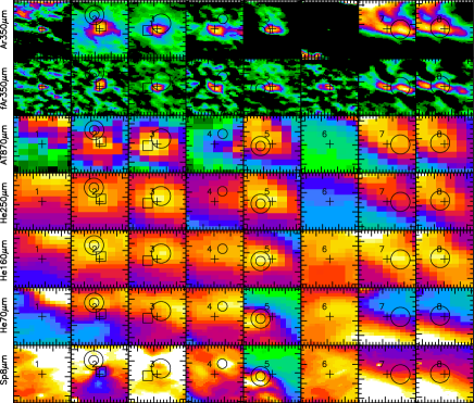
Figure 35: Same as Figure C1 but for the SDC328 field

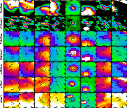
Figure 36: Figure C14 continued.

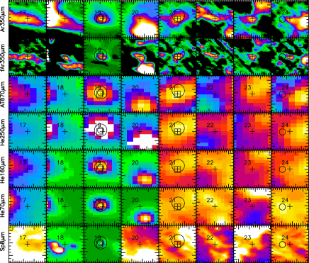
Figure 37: Figure C14 continued.

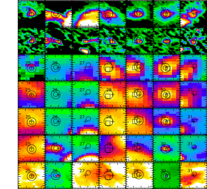
Figure 38: Figure C14 continued.

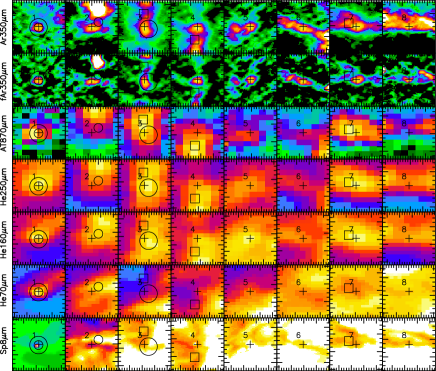
Figure 39: Same as Figure C1 but for the SDC340 field

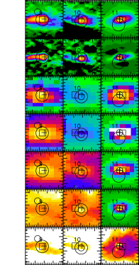
Figure 40: Figure C18 continued.

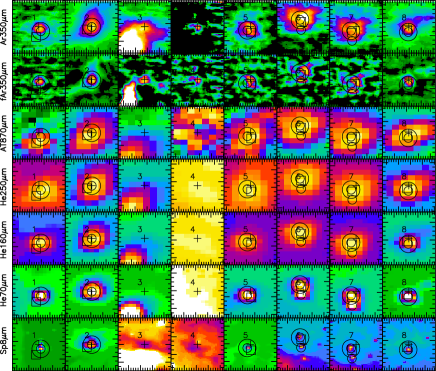
Figure 41: Same as Figure C1 but for the SDC343 field

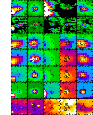
Figure 42: Figure C20 continued.

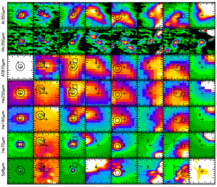
Figure 43: Same as Figure C1 but for the SDC345 field

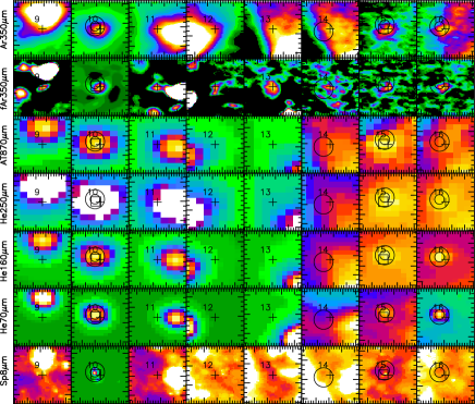
Figure 44: Figure C22 continued.

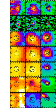
Figure 45: Figure C22 continued.

Appendix D Alternative dust temperature assumption

As mentioned in Sec. 6, all core temperatures displayed in Fig. 5 are derived from Eq. (5). This relationship has been partly inferred from the observed correlation between the internal temperature and the colour temperature of protostellar sources (see Fig. 4). The choice of applying Eq. (5) to both protostellar and starless sources is justified by the absence of correlation between the ratio $\overline{T}_{\rm{int}}/T_{\rm{col}}$ and the source internal luminosity. However, for completeness, we here show the mass vs. temperature diagram where the dust temperatures of starless sources are estimated using $T_{\rm{dust}}=T_{\rm{col}}$ while using $T_{\rm{dust}}=1.2\times 1.32\times T_{\rm{col}}$ for protostellar sources (as in Fig. 6). The 1.2 factor is taken from Eq. (5), while the 1.32 factor corresponds to the rescaling from 0.23 pc (the original resolution of the temperature data) to 0.1ṗc (see section 6). The resulting mass vs. temperature diagram is shown in Fig. 46.

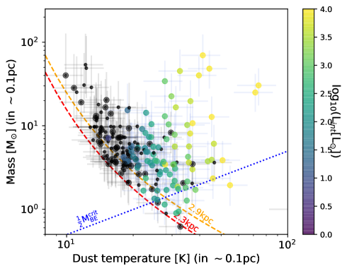
Figure 46: Same as Fig. 6 but with starless source’s temperatures estimated using $T_{\rm{dust}}=T_{\rm{col}}$ as opposed to $T_{\rm{dust}}=1.2T_{\rm{col}}$

Appendix E Models with $R_{\rm{core}}=1000$ AU

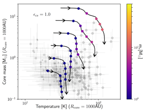
Figure 47: Core-fed models. Each track has been computed for a different initial core mass, from bottom to top ${m}_{\rm{core}}(t=0)=[0.5,1,2,4,8,16]$ M_⊙. The coloured symbols represent the position of the cores at times $t=[9\times 10^{3},9\times 10^{4},1.8\times 10^{5},2.7\times 10^{5},3.6\times 10^{5}]$ yr. The colour codes the stellar mass at these times as displayed by the colour bar. The background grey symbols are the ArTéMiS sources whose properties have been rescaled to 0.01pc (see text). Note that sources with $M_{\rm{gas}}<\frac{1}{2}M_{\rm{BE}}^{\rm{crit}}$ have been removed.

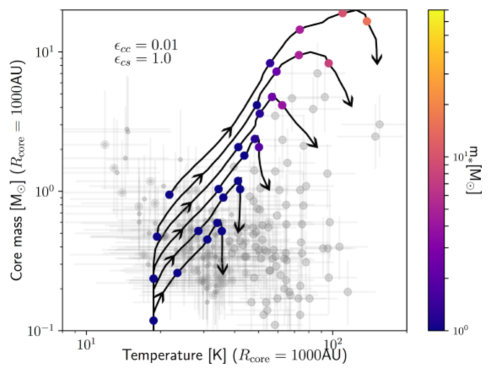
Figure 48: Clump-fed models. Each track has been computed for a different clump mass, from bottom to top $m_{\rm{clump}}=[100,200,400,800,1600,3200]$ M_⊙.The coloured symbols represent the position of the cores at times $t=[3\times 10^{4},3\times 10^{5},6\times 10^{5},9\times 10^{5},1.2\times 10^{6}]$ yr. The colour codes the stellar mass at these times as displayed by the colour bar. The background grey symbols are those presented in Fig. 47. Note that sources with $M_{\rm{gas}}<\frac{1}{2}M_{\rm{BE}}^{\rm{crit}}$ have been removed.

Fragmentation on scales of a couple of thousands AU scale (e.g. Bontemps et al., 2010; Motte et al., 2018a; Beuther et al., 2018), or even smaller scale (e.g. Palau et al., 2013) is routinely observed in massive star-forming regions. In an attempt to produce similar model/data comparisons as those presented in Figs. 7 and 8 but at a core scale of 0.01pc (i.e. $R_{\rm{core}}=1000$ AU) we rescaled the data as follows. For all sources, we assumed a density profile scaling as $\rho\propto r^{-2}$, which in practice implies a decrease of the core masses by a factor of 10 compared to the $R_{\rm{core}}=0.05$ pc case. Regarding the temperatures of protostellar sources, we used Eq. (1) with the relevant radius, which in practice means an increase of the temperature by a factor 2.1 compared to the $R_{\rm{core}}=0.05$ pc case. Finally, we leave unchanged the temperatures of starless sources. We here keep the same fractional temperature uncertainties of 20%, however these are most likely much larger. The resulting observed core temperatures and masses are displayed as grey symbols in Figs. 47 and 48.

Figure 47 shows a set of core-fed models, with 6 different initial cores masses, ${m}_{\rm{core}}(t=0)=[0.5,1,2,4,8,16]$ M_⊙. We kept the timescale $\tau_{\rm{core}}$ the same as in the $R_{\rm{core}}=0.05$ pc, but increased the core to star formation efficiency to $\epsilon_{cs}=1$, the maximum allowed for core-fed models. Unsurprisingly, the conclusions here are similar to those drawn from the $R_{\rm{core}}=0.05$ pc models, which is that they fail to explain the formation of the most massive stars (no massive prestellar cores), but may be compatible with the formation of intermediate-mass stars. The fact that one needs to use $\epsilon_{cs}=1$ to get a reasonable match with the data does show that massive star-forming cores on these sort of scales do need to accrete mass from radii that are larger than the last fragmentation scale. This is somewhat explicit given the low core masses.

Figure 48 on the other hand, shows clump-fed tracks with an initial core mass ${m}_{\rm{core}}(t=0)=0.1$ M_⊙, a core formation efficiency $\epsilon_{cc}=0.01$ and a core to star formation efficiency $\epsilon_{cs}=1$. Clump masses are identical to those used for the $R_{\rm{core}}=0.05$ pc models. Here again, as far as the most massive objects are concerned, we see that the clump-fed models are in better agreement with the observations. And similarly to the core-fed models, the use of $\epsilon_{cs}=1$ shows that larger scale accretion is required.

References

- Aguirre et al. (2011) Aguirre J. E., et al., 2011, ApJS, 192, 4
- Andre et al. (2000) Andre P., Ward-Thompson D., Barsony M., 2000, in Mannings V., Boss A. P., Russell S. S., eds, Protostars and Planets IV. p. 59 (arXiv:astro-ph/9903284)
- André et al. (2008) André P., et al., 2008, A&A, 490, L27
- André et al. (2010) André P., et al., 2010, A&A, 518, L102+
- André et al. (2014) André P., Di Francesco J., Ward-Thompson D., Inutsuka S. I., Pudritz R. E., Pineda J. E., 2014, in Beuther H., Klessen R. S., Dullemond C. P., Henning T., eds, Protostars and Planets VI. p. 27 (arXiv:1312.6232), doi:10.2458/azu_uapress_9780816531240-ch002
- André et al. (2016) André P., et al., 2016, A&A, 592, A54
- André et al. (2019) André P., Arzoumanian D., Könyves V., Shimajiri Y., Palmeirim P., 2019, A&A, 629, L4
- Arzoumanian et al. (2011) Arzoumanian D., et al., 2011, A&A, 529, L6+
- Arzoumanian et al. (2019) Arzoumanian D., et al., 2019, A&A, 621, A42
- Barnes et al. (2015) Barnes P. J., Muller E., Indermuehle B., O’Dougherty S. N., Lowe V., Cunningham M., Hernandez A. K., Fuller G. A., 2015, ApJ, 812, 6
- Beuther et al. (2013) Beuther H., et al., 2013, A&A, 553, A115
- Beuther et al. (2018) Beuther H., et al., 2018, A&A, 617, A100
- Bonnell et al. (2004) Bonnell I. A., Vine S. G., Bate M. R., 2004, MNRAS, 349, 735
- Bonnor (1956) Bonnor W. B., 1956, MNRAS, 116, 351
- Bontemps et al. (1996) Bontemps S., Andre P., Terebey S., Cabrit S., 1996, A&A, 311, 858
- Bontemps et al. (2010) Bontemps S., Motte F., Csengeri T., Schneider N., 2010, A&A, 524, A18
- Csengeri et al. (2014) Csengeri T., et al., 2014, A&A, 565, A75
- Csengeri et al. (2017) Csengeri T., et al., 2017, A&A, 600, L10
- Csengeri et al. (2018) Csengeri T., et al., 2018, A&A, 617, A89
- Duarte-Cabral et al. (2013) Duarte-Cabral A., Bontemps S., Motte F., Hennemann M., Schneider N., André P., 2013, A&A, 558, A125
- Dunham et al. (2008) Dunham M. M., Crapsi A., Evans II N. J., Bourke T. L., Huard T. L., Myers P. C., Kauffmann J., 2008, ApJS, 179, 249
- Ebert (1955) Ebert R., 1955, Z. Astrophys., 37, 217
- Elia et al. (2017) Elia D., et al., 2017, MNRAS, 471, 100
- Ellsworth-Bowers et al. (2013) Ellsworth-Bowers T. P., et al., 2013, ApJ, 770, 39
- Foster et al. (2013) Foster J. B., et al., 2013, Publ. Astron. Soc. Australia, 30, e038
- Giannetti et al. (2015) Giannetti A., Wyrowski F., Leurini S., Urquhart J., Csengeri T., Menten K. M., Bronfman L., van der Tak F. F. S., 2015, A&A, 580, L7
- Hildebrand (1983) Hildebrand R. H., 1983, QJRAS, 24, 267
- Hosokawa & Omukai (2009) Hosokawa T., Omukai K., 2009, ApJ, 691, 823
- Inutsuka & Miyama (1997) Inutsuka S.-i., Miyama S. M., 1997, ApJ, 480, 681
- Könyves et al. (2015) Könyves V., et al., 2015, A&A, 584, A91
- Könyves et al. (2020) Könyves V., et al., 2020, A&A, 635, A34
- Ladjelate et al. (2020) Ladjelate B., et al., 2020, arXiv e-prints, p. arXiv:2001.11036
- Lee et al. (2017) Lee Y.-N., Hennebelle P., Chabrier G., 2017, ApJ, 847, 114
- Louvet et al. (2019) Louvet F., et al., 2019, A&A, 622, A99
- McKee & Offner (2010) McKee C. F., Offner S. S. R., 2010, ApJ, 716, 167
- Men’shchikov et al. (2010) Men’shchikov A., et al., 2010, A&A, 518, L103
- Molinari et al. (2008) Molinari S., Pezzuto S., Cesaroni R., Brand J., Faustini F., Testi L., 2008, A&A, 481, 345
- Molinari et al. (2010) Molinari S., et al., 2010, A&A, 518, L100+
- Molinari et al. (2016) Molinari S., et al., 2016, A&A, 591, A149
- Moore et al. (2015) Moore T. J. T., et al., 2015, MNRAS, 453, 4264
- Motte et al. (1998) Motte F., Andre P., Neri R., 1998, A&A, 336, 150
- Motte et al. (2007) Motte F., Bontemps S., Schilke P., N., Menten K. M., Broguière D., 2007, A&A, 476, 1243
- Motte et al. (2018a) Motte F., et al., 2018a, Nature Astronomy, 2, 478
- Motte et al. (2018b) Motte F., Bontemps S., Louvet F., 2018b, ARA&A, 56, 41
- Myers (2009) Myers P. C., 2009, ApJ, 700, 1609
- Myers (2012) Myers P. C., 2012, ApJ, 752, 9
- Offner & McKee (2011) Offner S. S. R., McKee C. F., 2011, ApJ, 736, 53
- Palau et al. (2013) Palau A., et al., 2013, ApJ, 762, 120
- Peretto & Fuller (2009) Peretto N., Fuller G. A., 2009, A&A, 505, 405
- Peretto et al. (2006) Peretto N., André P., Belloche A., 2006, A&A, 445, 979
- Peretto et al. (2013) Peretto N., et al., 2013, A&A, 555, A112
- Peretto et al. (2016) Peretto N., Lenfestey C., Fuller G. A., Traficante A., Molinari S., Thompson M. A., Ward-Thompson D., 2016, A&A, 590, A72
- Ragan et al. (2012) Ragan S. E., Heitsch F., Bergin E. A., Wilner D., 2012, ApJ, 746, 174
- Reid et al. (2009) Reid M. J., et al., 2009, ApJ, 700, 137
- Reid et al. (2014) Reid M. J., et al., 2014, ApJ, 783, 130
- Revéret et al. (2014) Revéret V., et al., 2014, The ArTéMiS wide-field sub-millimeter camera: preliminary on-sky performance at 350 microns. p. 915305, doi:10.1117/12.2055985
- Rosolowsky et al. (2008) Rosolowsky E. W., Pineda J. E., Kauffmann J., Goodman A. A., 2008, ApJ, 679, 1338
- Sanhueza et al. (2019) Sanhueza P., et al., 2019, ApJ, 886, 102
- Schneider et al. (2010) Schneider N., Csengeri T., Bontemps S., Motte F., Simon R., Hennebelle P., Federrath C., Klessen R., 2010, A&A, 520, A49
- Schuller et al. (2009) Schuller F., et al., 2009, A&A, 504, 415
- Smith et al. (2009) Smith R. J., Longmore S., Bonnell I., 2009, MNRAS, 400, 1775
- Svoboda et al. (2019) Svoboda B. E., et al., 2019, ApJ, 886, 36
- Terebey et al. (1993) Terebey S., Chandler C. J., Andre P., 1993, ApJ, 414, 759
- Urquhart et al. (2014) Urquhart J. S., et al., 2014, MNRAS, 443, 1555
- Vázquez-Semadeni et al. (2019) Vázquez-Semadeni E., Palau A., Ballesteros-Paredes J., Gómez G. C., Zamora-Avilés M., 2019, MNRAS, 490, 3061
- Wang et al. (2010) Wang P., Li Z.-Y., Abel T., Nakamura F., 2010, ApJ, 709, 27