Corrugation Process and $\epsilon$-Isometric Maps

Abstract.

Convex Integration is a theory developed in the ’70s by M. Gromov. This theory allows to solve families of differential problems satisfying some convex assumptions. From a subsolution, the theory iteratively builds a solution by applying a series of convex integrations. In a previous paper [6], we proposed to replace the usual convex integration formula by a new one called Corrugation Process. This new formula is of particular interest when the differential problem under consideration has the property of being of Kuiper. In this paper, we consider the differential problem of $\epsilon$-isometric maps and we prove that it is Kuiper in codimension 1. As an application, we construct $\epsilon$-isometric maps from a short map having a conical singularity.

1. General introduction

1.1. The Nash-Kuiper Theorem

A map $f:(M,g)\rightarrow\mathbb{E}^{n}$ between a Riemannian manifolds $(M,g)$ and the Euclidean space $\mathbb{E}^{n}=(\mathbb{R}^{n},\langle\cdot,\cdot\rangle)$ is said to be isometric if $g=f^{*}\langle\cdot,\cdot\rangle.$ It is said to be strictly short if $g-f^{*}\langle\cdot,\cdot\rangle$ is positive definite (as usual $f^{*}h$ denotes the pullback of the metric $h$ by $f$). In other words, the length of the image of any curve in $M$ by a strictly short map is shorter than the length of the curve in $M$. The $C^{1}$ embedding theorem of Nash and Kuiper states that close to every strictly short map lies a $C^{1}$-isometric map:

Theorem 1 ([4, 3]).

Let $(M^{m},g)$ be a compact Riemannian manifold and let $f_{0}:(M^{m},g)\rightarrow(\mathbb{R}^{n},\langle\cdot,\cdot\rangle)$, with $n>m$, be a strictly short embedding. Then for any $\epsilon>0$ there exists a $C^{1}$-isometric embedding $f:(M^{m},g)\rightarrow(\mathbb{R}^{n},\langle\cdot,\cdot\rangle)$ such that, $\sup_{x}\|f(x)-f_{0}(x)\|<\epsilon.$

The proof considers an increasing sequence of metrics $g_{k}$ converging toward $g$ and a decreasing sequence $\epsilon_{k}$ converging toward $0$. A sequence of maps $f_{1},\ldots$, $f_{k}$, $\ldots$ is then iteratively built such that, for each $k$, $f_{k}$ is an $\epsilon_{k}$-isometric map from $(M,g_{k})$ to $\mathbb{E}^{n}$ i. e.

$$\|g_{k}-f_{k}^{*}h\|<\epsilon_{k}.$$

Parameters of the construction are chosen to insure the $C^{1}$ convergence of the sequence $(f_{k})_{k}$ so that the limit map $f_{\infty}$ is isometric.

1.2. Differential relations

We now introduce the formalism of Gromov’s Convex Integration Theory [2]. This theory can be seen as a wide generalization of Nash’s approach. It provides a powerful tool to solve a large family of differential constraints. We denote by

$$J^{1}(M,W):=\{(x,y,L)\,\,|\,\,x\in M,\,\,y\in W,\,\,L:T_{x}M\rightarrow T_{y}W\mbox{ a linear map}\}.$$

the $1$-jet space of $C^{1}$ maps between $M$ and $W$. Every $C^{1}$-map $f$ gives rise to a section $j^{1}f:x\mapsto(x,f(x),df_{x})$ of $J^{1}(M,W)$ called the 1-jet of $f$. For any section $\mathfrak{S}_{0}:x\mapsto(x,f_{0}(x),L_{x})$ we denote by $f_{0}=\mathrm{bs}\;\;\mathfrak{S}_{0}$ its base map.

A differential relation $\mathcal{R}$ is any subset of the $1$-jet space $J^{1}(M,W)$. For instance, the $\epsilon$-isometric condition defines the differential relation $\mathcal{I\!\!s}(\epsilon)$ of $\epsilon$-isometric maps:

$$\mathcal{I\!\!s}(\epsilon):=\{(x,y,L)\,\,|\,\,\|g_{x}-L^{*}h_{y}\|<\epsilon\}$$

where $L^{*}h$ denotes the pullback by $L$ of the metric $h$. Observe that, as a topological subspace, $\mathcal{I\!\!s}(\epsilon)$ is open.

Definition 2.

Let $\mathfrak{S}:M\rightarrow J^{1}(M,W)$ be a section. We say that $\mathfrak{S}$ is a formal solution of $\mathcal{R}$ if the image of $\mathfrak{S}$ lies in $\mathcal{R}$. Moreover, if there exists a $C^{1}$-map $f:M\rightarrow W$ such that $j^{1}f=\mathfrak{S}$, we say that $\mathfrak{S}$ is a holonomic solution of $\mathcal{R}$.

For instance, building an $\epsilon$-isometric map $f$ is equivalent to finding a holonomic solution $j^{1}f$ of $\mathcal{I\!\!s}(\epsilon)$.

Under some topological and convex assumptions on $\mathcal{R}$, the Convex Integration Theory allows to deform a formal solution $\mathfrak{S}_{0}$ to a holonomic one. Each convex integration modifies the 1-jet of a formal solution $(x_{0},f_{0},L_{0})$ in a given direction $u$ to obtain a new formal solution $\mathfrak{S}=(x,f,L)$ such that $L(u)=df(u)$. Loosely speaking $\mathfrak{S}$ is "partially holonome in the direction $u$". Here is how it works for $M=[0,1]^{m}$ and $W=\mathbb{E}^{n}$. In this case a formal solution writes

$$\mathfrak{S}_{0}:x\mapsto(x,f_{0}(x),v_{1}(x),\ldots,v_{m}(x))\in\mathcal{R}$$

where we have identified the 1-jet space with the product

$$J^{1}([0,1]^{m},\mathbb{R}^{n})=[0,1]^{m}\times\mathbb{R}^{n}\times(\mathbb{R}^{n})^{m}$$

and $\mathfrak{S}_{0}$ is holonomic if there exists a map $f$ such that

$$\mathfrak{S}_{0}=j^{1}f:x\mapsto(x,f(x),\partial_{1}f(x),\ldots,\partial_{m}f(x)).$$

From a formal solution $\mathfrak{S}_{0}$, the Convex Integration Theory builds a finite sequence of formal solutions $\mathfrak{S}_{k}$ such that for every $k\in\{1,\ldots,m\}$ we have

$$\mathfrak{S}_{k}:x\mapsto(x,f_{k}(x),\partial_{1}f_{k}(x),\ldots,\partial_{k}f_{k}(x),v_{k+1}(x),\ldots,v_{m}(x))\in\mathcal{R}.$$

In particular

$$\mathfrak{S}_{m}=j^{1}f_{m}:x\mapsto(x,f_{m}(x),\partial_{1}f_{m}(x),\ldots,\partial_{m}f_{m}(x))$$

is a holonomic solution of $\mathcal{R}$.

1.3. Corrugation Process

To build the sequence $(\mathfrak{S}_{k})_{k}$, we propose in [6] to replace the usual formula of the Convex Integration Theory by another one, called Corrugation Process:

Definition 3.

Let $f_{0}:[0,1]^{m}\rightarrow\mathbb{R}^{n}$ be a map, $\partial_{j}$ be a direction, $\gamma:[0,1]^{m}\times\mathbb{R}/\mathbb{Z}\rightarrow\mathbb{R}^{n}$ be a loop family and $N\in\;]0,+\infty[$. We define the map $f_{1}:[0,1]^{m}\rightarrow\mathbb{R}^{n}$ by

(1) $$f_{1}(x):=f_{0}(x)+\frac{1}{N}\int_{s=0}^{Nx_{j}}\gamma(x,s)-\overline{\gamma}(x)ds$$

where $\overline{\gamma}(x)=\int_{0}^{1}\gamma(x,s)ds$ denotes the average of the loop $t\mapsto\gamma(x,t)$. We say that $f_{1}$ is obtained from $f_{0}$ by a Corrugation Process in the direction $\partial_{j}$ and we denote $f_{1}=CP_{\textstyle{\textup{$\gamma$}}}(f_{0},\partial_{j},N)$.

The Corrugation Process satisfies the following three properties which are at the basis of the Convex Integration Theory [5].

Proposition 4 ([6]).

The map $f_{1}=CP_{\textstyle{\textup{$\gamma$}}}(f_{0},\partial_{j},N)$ satisfies

• $\|f_{0}-f_{1}\|_{C^{0}}=O(1/N)$,

• $\|\partial_{i}f_{0}-\partial_{i}f_{1}\|_{C^{0}}=O(1/N)$ for every $i\neq j$.

Moreover if $\forall x\in[0,1]^{m}$ we have $\partial_{j}f_{0}(x)=\overline{\gamma}(x)$ then

• $\partial_{j}f_{1}(x)=\gamma(x,Nx_{j})+O(1/N)$ for all $x\in[0,1]^{m}$.

Provided that $N$ is large enough, this proposition shows that the Corrugation Process allows to modify the $j$th partial derivative while keeping the other derivatives under control. Consequently, this formula performs the deformations required to build the sequence $(\mathfrak{S}_{k})_{k}$ provided $\gamma$ has values in a well chosen region. For more details and for a proof of this proposition see [6]. We give below a coordinate free expression of the Corrugation Process:

Definition 5.

Let $f_{0}:U\rightarrow(W,h)$ be a map from an open set $U\subset M$, $\pi:U\rightarrow\mathbb{R}$ be a submersion and $\gamma:U\times\mathbb{R}/\mathbb{Z}\rightarrow f_{0}^{*}TW$ be a loop family such that $\gamma(x,.):\mathbb{R}/\mathbb{Z}\rightarrow f_{0}^{*}TW_{x}$ for every $x\in U$. The map defined by Corrugation Process is defined by

$$f_{1}=CP_{\textstyle{\textup{$\gamma$}}}(f_{0},\pi,N):x\mapsto\exp_{f_{0}(x)}\Big{(}\frac{1}{N}\int_{t=0}^{N\pi(x)}\gamma(x,t)-\overline{\gamma}(x)dt\Big{)}$$

where $\exp:TW\rightarrow W$ is the exponential map induced by the metric $h$.

1.4. Subsolutions

Subsolutions are a refinement of the notion of formal solution. This refinement is needed to ensure the existence of a loop family $\gamma$ whose its values is chosen in an appropriate region and whose its average is the partial derivative $\partial_{j}f_{0}$ under consideration (see property $(P_{3})$ of Proposition 4).

Let $\mathcal{R}$ be a differential relation, $\sigma=(x,y,L)\in\mathcal{R}$ and $(\lambda,u)\in T_{x}^{*}M\times T_{x}M$ such that $\lambda(u)=1$. We set

$$\mathcal{R}(\sigma,\lambda,u):=Conn_{L(u)}\{v\in T_{y}W\;|\;(x,y,L+(v-L(u))\otimes\lambda)\in\mathcal{R}\}$$

where $Conn_{a}A$ denotes the path connected component of $A$ that contains $a$. We say that $\mathcal{R}(\sigma,\lambda,u)$ is the slice of $\mathcal{R}$ over $\mathfrak{S}$ with respect to $(\lambda,u)$. Note that the linear map $L+(v-L(u))\otimes\lambda$ coincides with $L$ over $\ker\lambda$ and maps $u$ to $v$. We then denote by $\mathrm{IntConv}\;\mathcal{R}(\sigma,\lambda,u)$ the interior of the convex hull of $\mathcal{R}(\sigma,\lambda,u).$

Definition 6.

Let $U\subset M$, $\pi:U\rightarrow\mathbb{R}$ be a submersion and $u:U\rightarrow TM$ be a vector field such that $d\pi_{x}(u_{x})=1$. Let $x\mapsto\mathfrak{S}(x)=(x,f_{0}(x),L(x))$ be a formal solution of $\mathcal{R}$ over $U$. If for every $x$ in $U$ the base map $f_{0}=\mathrm{bs}\;\mathfrak{S}$ satisfies

$$df_{0}(u_{x})\in\mathrm{IntConv}\;\mathcal{R}(\mathfrak{S}(x),d\pi_{x},u_{x})$$

then the formal solution $\mathfrak{S}$ is called a subsolution of $\mathcal{R}$ with respect to $(d\pi,u)$.

In the case where $U=[0,1]^{m}$, $W=\mathbb{R}^{n}$, $\pi(x)=x_{j}$ and $u=\partial_{j}$, the condition of the definition means that $\partial_{j}f_{0}(x)$ lies in the interior of the convex hull of

$$\mathcal{R}(\sigma,dx_{j},\partial_{j})=Conn_{v_{j}}\{t\in\mathbb{R}^{n}\;|\;(x,f_{0}(x),v_{1},\ldots,v_{j-1},t,v_{j+1},\ldots,v_{m})\in\mathcal{R}\}.$$

From a subsolution $\mathfrak{S}$ of $\mathcal{R}$ with respect to $(d\pi,u)$ the Convex Integration Theory builds a map $f_{1}$ whose derivative along $u_{x}$ lies in the slice $\mathcal{R}(\mathfrak{S}(x),d\pi_{x},u_{x})$:

Lemma 7.

Let $\mathcal{R}$ be an open differential relation and let $\mathfrak{S}$ be a subsolution of $\mathcal{R}$ with respect to $(d\pi,u)$ and with base map $f_{0}=\mathrm{bs}\;\;\mathfrak{S}$. Then there exists a loop family $\gamma$ such that for every $x\in U$ we have $\overline{\gamma}(x)=df_{0}(u_{x})$ and for every $(x,t)\in U\times\mathbb{R}/\mathbb{Z}$ the image of $\gamma$ lies in $\mathcal{R}(\mathfrak{S}(x),d\pi_{x},u_{x})$. If we set $f_{1}:=CP_{\textstyle{\textup{$\gamma$}}}(f_{0},\pi,N)$ for this loop family $\gamma$, we have

$$\forall x\in U,\;\;\;\;\;df_{1}(u_{x})\in\mathcal{R}(\mathfrak{S}(x),d\pi_{x},u_{x})$$

for $N$ large enough.

Proof.– The existence of $\gamma$ follows the Integral Representation Lemma of the Convex Integration Theory of Gromov ([2, p169] or [5, p29]). The property on $df_{1}(u_{x})$ is a direct consequence of point $(P_{3})$ of Proposition 4. , $\square$

1.5. Kuiper relations

In the usual approach, the family of loops $\gamma$ is constructed a posteriori once the subsolution $\mathfrak{S}$ given. However the construction of a holonomic solution often requires to repeat the Corrugation Process in several directions $\partial_{j}$ and consequently needs to re-build at each step the loop family $\gamma$ on a different subsolution at each time. In [6], we propose to simplify this approach by constructing a bigger loop family $\gamma$$\blacksquare$ $\gamma$ that could be used indifferently regardless of the subsolution. This simplification leads to introduce the notion of surrounding loop family and then the notion of Kuiper relation.

Basically, a surrounding family is a family of loops lying inside $\mathcal{R}$ which is double indexed by its base point $\sigma$ and its average $w$ and where $(\sigma,w)$ are allowed to vary in the largest possible space, that is, inside

$$\mathrm{IntConv}(\mathcal{R},d\pi,u):=\{(\sigma,w)\in p_{y}^{*}TW\;|\;w\in\mathrm{IntConv}\;\mathcal{R}(\sigma,d\pi_{x},u_{x})\}.$$

In that definition, $p_{y}^{*}TW$ is the bundle over $\mathcal{R}$ induced by the projection $p_{y}:\mathcal{R}\rightarrow W$, $\sigma=(x,y,L)\mapsto y.$

Definition 8.

Let $\mathcal{R}$ be a differential relation of $J^{1}(U,W)$. We say that a loop family

$$\begin{array}[]{lclc}\textstyle{\textup{\raisebox{1.7pt}{$\gamma$\raisebox{-6.5pt}{{\color[rgb]{1,1,1}$\blacksquare$}}} $\gamma$}}:&\mathrm{IntConv}(\mathcal{R},d\pi,u)&\longrightarrow&C^{0}(\mathbb{R}/\mathbb{Z},TW)\\ &(\sigma,w)&\longmapsto&\textstyle{\textup{\raisebox{1.7pt}{$\gamma$\raisebox{-6.5pt}{{\color[rgb]{1,1,1}$\blacksquare$}}} $\gamma$}}(\sigma,w)(\cdot)\end{array}$$

is surrounding with respect to $(d\pi,u)$ if for every $(\sigma,w)$ we have

• $t\mapsto\textstyle{\textup{\raisebox{1.7pt}{$\gamma$\raisebox{-6.5pt}{{\color[rgb]{1,1,1}$\blacksquare$}}} $\gamma$}}(\sigma,w)(t)$ is a loop in $\mathcal{R}(\sigma,d\pi_{x},u_{x})$,

• the average of $t\mapsto\textstyle{\textup{\raisebox{1.7pt}{$\gamma$\raisebox{-6.5pt}{{\color[rgb]{1,1,1}$\blacksquare$}}} $\gamma$}}(\sigma,w)(t)$ is $w$,

• there exists a continuous homotopy $H:\mathrm{IntConv}(\mathcal{R},d\pi,u)\times[0,1]\rightarrow TW$ such that $H(\sigma,w,0)=\textstyle{\textup{\raisebox{1.7pt}{$\gamma$\raisebox{-6.5pt}{{\color[rgb]{1,1,1}$\blacksquare$}}} $\gamma$}}(\sigma,w)(0)$, $H(\sigma,w,1)=L(u_{x})$ and $H(\sigma,w,t)\in\mathcal{R}(\sigma,d\pi_{x},u_{x})$ for all $t\in\,[0,1].$

Note that point $(3)$ is a homotopic property needed to state a potential $h$-principle for $\mathcal{R}$.

Then for any subsolution $\mathfrak{S}=(x,f_{0},L)$ we choose the loop family

$$\gamma(x,t):=\textstyle{\textup{\raisebox{1.7pt}{$\gamma$\raisebox{-6.5pt}{{\color[rgb]{1,1,1}$\blacksquare$}}} $\gamma$}}(\mathfrak{S}(x),df_{0}(u_{x}))(t)\in\mathcal{R}(\sigma,d\pi_{x},u_{x})$$

for every $(x,t)\in U\times\mathbb{R}/\mathbb{Z}$, and we write $CP_{\textstyle{\textup{\raisebox{1.7pt}{$\gamma$\raisebox{-6.5pt}{{\color[rgb]{1,1,1}$\blacksquare$}}} $\gamma$}}}(\mathfrak{S},\pi,N):=CP_{\textstyle{\textup{$\gamma$}}}(f_{0},\pi,N).$

We would like to ensure that all loops $\textstyle{\textup{\raisebox{1.7pt}{$\gamma$\raisebox{-6.5pt}{{\color[rgb]{1,1,1}$\blacksquare$}}} $\gamma$}}(\sigma,w)$ share the same pattern.

Definition 9.

Let $p,q>0$ be two natural numbers and $A\subset\mathbb{R}^{q}$ be a parameter space. A family of $1$-periodic curves $c:A\times\mathbb{R}/\mathbb{Z}\rightarrow\mathbb{R}^{p}$ is said to be a pattern.

We denote by $E\rightarrow W$ the fiber bundle over $W$ with fiber $\mathcal{L}(\mathbb{R}^{p},T_{y}W)=(\mathbb{R}^{p})^{*}\otimes T_{y}W$ and we consider its pull back by the projection $q:\mathrm{IntConv}(\mathcal{R},d\pi,u)\rightarrow W$, $(\sigma,w)\mapsto y$. A section $\mathcal{e}$ of $q^{*}E$ defines a family of linear maps $\mathcal{e}(\sigma,w):\mathbb{R}^{p}\rightarrow T_{y}W$.

Definition 10.

Let $c$ be a loop pattern. If there exist a surrounding loop family $\textstyle{\textup{\raisebox{1.7pt}{$\gamma$\raisebox{-6.5pt}{{\color[rgb]{1,1,1}$\blacksquare$}}} $\gamma$}}:\mathrm{IntConv}(\mathcal{R},d\pi,u)\rightarrow C^{0}(\mathbb{R}/\mathbb{Z},TW)$ with respect to $(d\pi,u)$, a section $\mathcal{e}$ of $q^{*}E\rightarrow\mathrm{IntConv}(\mathcal{R},d\pi,u)$ and a map ${\bf a}:\mathrm{IntConv}(\mathcal{R},d\pi,u)\rightarrow A$ such that, for all $((\sigma,w),t)\in\mathrm{IntConv}(\mathcal{R},d\pi,u)\times\mathbb{R}/\mathbb{Z}$,

$$\textstyle{\textup{\raisebox{1.7pt}{$\gamma$\raisebox{-6.5pt}{{\color[rgb]{1,1,1}$\blacksquare$}}} $\gamma$}}(\sigma,w)(t)=\displaystyle\mathcal{e}(\sigma,w)\circ c({\bf a}(\sigma,w),t)$$

we then say that $\mathcal{R}$ is a Kuiper relation with respect to $(c,d\pi,u)$.

If $(c_{1},\ldots,c_{p})$ denote the components of $c$ in the standard basis of $\mathbb{R}^{p}$ and if $\textbf{e}_{1},\ldots,\textbf{e}_{p}$ denote the image of this basis by $\mathcal{e}$, the above definition writes

$$\textstyle{\textup{\raisebox{1.7pt}{$\gamma$\raisebox{-6.5pt}{{\color[rgb]{1,1,1}$\blacksquare$}}} $\gamma$}}(\sigma,w)(t)=\displaystyle\sum_{i=1}^{p}c_{i}({\bf a}(\sigma,w),t)\,{\bf e}_{i}(\sigma,w).$$

We denote the periodic primitive of the $c_{i}$’s by

$$C_{i}(a,t)=\int_{s=0}^{t}c_{i}(a,s)-\overline{c_{i}}(a)ds.$$

Proposition 11.

Let $c$ be a loop pattern, $\mathcal{R}$ be an open Kuiper relation with respect to $(c,d\pi,u)$, $\mathfrak{S}=(x,f_{0},L_{0})$ be a subsolution and $\gamma$$\blacksquare$ $\gamma$ be a $c$-shaped surrounding loop family. Then $f_{1}=CP_{\textstyle{\textup{\raisebox{1.7pt}{$\gamma$\raisebox{-6.5pt}{{\color[rgb]{1,1,1}$\blacksquare$}}} $\gamma$}}}(\mathfrak{S},\pi,N)$ has the following analytic expression

(3) $$f_{1}(x) = \exp_{f_{0}(x)}\left(\frac{1}{N}\sum_{i=1}^{p}C_{i}(a(x),N\pi(x))e_{i}(x)\right)$$

where $a(x):=\textbf{a}(\mathfrak{S}(x),df_{0}(u_{x}))$, $e(x):=\textbf{e}(\mathfrak{S}(x),df_{0}(u_{x}))$ and $x\in U$. Moreover, if $N$ is large enough, the section

$$x\mapsto\mathfrak{S}_{1}:=(x,f_{1},L_{1}=L_{0}+(df_{1}(u_{x})-L_{0}(u_{x}))\otimes d\pi)$$

is a formal solution of $\mathcal{R}$.

In the case where $U=[0,1]^{m}$, $W=\mathbb{R}^{n}$, $\pi(x)=x_{j}$ and $u=\partial_{j}$ the map $f_{1}=CP_{\textstyle{\textup{\raisebox{1.7pt}{$\gamma$\raisebox{-6.5pt}{{\color[rgb]{1,1,1}$\blacksquare$}}} $\gamma$}}}(\mathfrak{S},\partial_{j},N)$ is given by

$$f_{1}(x)=f_{0}(x)+\frac{1}{N}\Big{(}\sum_{i=1}^{p}C_{i}(a(x),Nx_{j})e_{i}(x)\Big{)}.$$

In [6] the reader will find a proof of the proposition as well as examples of Kuiper relations. In the next section, we prove that the relation of $\epsilon$-isometric maps is Kuiper in codimension one.

2. The relation of $\epsilon$-isometric maps

In this article, we prove the following theorem:

Theorem 12.

Let $M$ and $W$ be orientable Riemannian manifolds such that $\dim W=\dim M+1$. For every $\epsilon>0$, the relation $\mathcal{I\!\!s}(\epsilon)$ is a Kuiper relation.

The key point of the proof of this theorem is to build a loop family $\gamma$$\blacksquare$ $\gamma$ $c$-shaped for all couples $(\sigma,w)$ such that $\sigma$ belongs to $\mathcal{I\!\!s}(\epsilon)$ and $w$ belongs to the convex hull of the slice $\mathcal{I\!\!s}(\epsilon)(\sigma,\lambda,u)$, for some $\lambda$, $u$. To understand the slice $\mathcal{I\!\!s}(\epsilon)(\sigma,\lambda,u)$ and its convex hull, we first present its geometric description and a description of its subsolutions. We then give a proof of Theorem 12.

2.1. Geometric description of the relation of isometric maps

The relation of $\epsilon$-isometric maps is a thickening of the relation of isometric maps

$$\mathcal{I\!\!s}:=\{(x,y,L)\,\,|\,\,g=L^{*}h\}\subset J^{1}(M,W)$$

where $g$ is a metric of $M$ and $L^{*}h$ is the pullback by $L$ of the metric $h$ of $W$. So in this paragraph we give a geometric description of the relation of isometric maps. Such a description can be found in [2, p202] or [5, p194]. For the sake of completeness we recall this description here in the coordinate-free case and we give some extra details needed for our construction of a surrounding loop family of the relation of $\epsilon$-isometric maps.

Let $\sigma=(x,y,L)\in\mathcal{I\!\!s}$. Let $\lambda\in T_{x}^{*}M$ and $u\in T_{x}M$ such that $\lambda(u)=1$. For every $v\in T_{y}W$, we set $L_{v}:=L+(v-L(u))\otimes\lambda$. We have

$$\mathcal{I\!\!s}(\sigma,\lambda,u) := Conn_{L(u)}\{v\in T_{y}W\;|\;(x,y,L_{v})\in\mathcal{I\!\!s}\}$$

$$= Conn_{L(u)}\{v\in T_{y}W\;|\;g_{x}=L_{v}^{*}h_{y}\}.$$

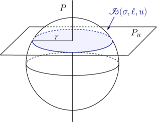
Figure 1. The slice $\mathcal{I\!\!s}(\sigma,\lambda,u)$ and its convex hull: the $(n-m)$-dimensional sphere in dark blue is $\mathcal{I\!\!s}(\sigma,\lambda,u)$ and the convex hull $\mathrm{IntConv}\,\mathcal{I\!\!s}(\sigma,\lambda,u)$ is the $(n-m+1)$-ball in light blue. $P$ denotes the $(m-1)$-plane $L(\ker\lambda)$

Note that, by the definition of $L_{v}$, we have $L_{v}(u)=v$ and for every $u_{0}\in\ker\lambda$ we have $L_{v}(u_{0})=L(u_{0})$, in particular $L_{v}(\ker\lambda)=L(\ker\lambda)$. Let $w_{1}=\alpha_{1}u+a_{1}$ and $w_{2}=\alpha_{2}u+a_{2}$ with $\alpha_{1},\alpha_{2}\in\mathbb{R}$ and $a_{1},a_{2}\in\ker\lambda$. As $g=L^{*}h$, we have

$$(g-L_{v}^{*}h)(w_{1},w_{2}) = \alpha_{1}\alpha_{2}(g(u,u)-h(v,v))$$

$$+\alpha_{1}h(L(u)-v,L(a_{2}))+\alpha_{2}h(L(u)-v,L(a_{1})).$$

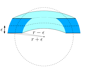
Figure 2. Illustration of a slice of $\mathcal{I\!\!s}(\epsilon)$: in blue, a piece of $\mathcal{I\!\!s}(\epsilon)(\sigma,\lambda,u)$. The slice $\mathcal{I\!\!s}(\epsilon)(\sigma,\lambda,u)$ is obtained as the intersection of the $\epsilon$-thickening of the $(n-m+1)$-plane $P_{u}$ and the $\epsilon$-thickening of the $(n-m)$-sphere $S_{u}$ of radius $r$.

From this expression it is readily seen that $g=L_{v}^{*}h$ if and only if $g(u,u)=h(v,v)$ and $v\in L(u)+L(\ker\lambda)^{\perp}$. So $v$ lies inside the $(n-1)$-dimensional sphere $S_{u}$ of radius $\|u\|_{g}$ and inside the affine $(n-m+1)$-plane

$$P_{u}:=L(u)+L(\ker\lambda)^{\perp}.$$

Thus $\mathcal{I\!\!s}(\sigma,\lambda,u)=S_{u}\cap P_{u}$ is a $(n-m)$-dimensional sphere of $T_{y}W$ and its convex hull is a ball of the same dimension (see Figure 1). Since we have assumed $n>m$, the space $\mathcal{I\!\!s}(\sigma,\lambda,u)$ is arc-connected. Since $\mathcal{I\!\!s}(\sigma,\lambda,u)$ is a $(n-m)$-dimensional sphere, $\mathrm{IntConv}\,\mathcal{I\!\!s}(\sigma,\lambda,u)$ is a $(n-m+1)$-ball of $P_{u}$.

So a slice of the relation of $\epsilon$-isometric maps is a thickening of $\mathcal{I\!\!s}(\sigma,\ell,u)$ (see Figure 2).

2.2. Characterization of subsolutions of the relation of isometric maps

Let $\mbox{proj}_{0}$ be the orthogonal projection on $\ker\lambda$ in $T_{x}M$ and $\mbox{proj}_{P}$ be the orthogonal projection on $P=L(\ker\lambda)$ in $T_{y}W$. We characterize subsolutions of $\mathcal{I\!\!s}$ with respect to $(d\pi,u)$, for a submersion $\pi:U\subset M\rightarrow\mathbb{R}$ and a tangent vector field $u:U\rightarrow TM$ such that $d\pi(u)=1$, in the following proposition:

Proposition 13.

Let $f_{0}:M\rightarrow W$ be a $C^{1}$-map and $P:=df_{0}(\ker d\pi)$ such that $\dim\;P(x)=m-1$ for all $x\in U$. If $f_{0}$ satisfies $g|_{\ker d\pi}=f_{0}^{*}h|_{\ker d\pi}$, then a section

$$x\mapsto\mathfrak{S}(x)=(x,f_{0}(x),L_{x}:=(df_{0})_{x}+(v_{x}-(df_{0})_{x}(u_{x}))\otimes d\pi_{x})$$

is a formal solution of $\mathcal{I\!\!s}$ with respect to $(d\pi,u)$ if and only if, for every $x$, the vector $v_{x}$ can be written in the form $v_{x}=\mbox{proj}_{P(x)}L_{x}(u_{x})+\tau_{x}$ where $\tau_{x}\in P(x)^{\perp}$ and $\|\tau_{x}\|_{h}=r(x)=\sqrt{\|u_{x}\|_{g}^{2}-\|\mbox{proj}_{0}u_{x}\|_{g}^{2}}$.

Proof.– Recall that $v_{x}\in\mathcal{I\!\!s}(\mathfrak{S}(x),d\pi_{x},u_{x})$ if and only if $v_{x}\in S_{u(x)}\cap P_{u(x)}$ i.e.

$$\|v_{x}\|_{h}^{2}=\|u_{x}\|_{g}^{2}\,\,\mbox{ and }\,\,\mbox{proj}_{P(x)}v_{x}=\mbox{proj}_{P(x)}L(u_{x}).$$

Decomposing $v_{x}$ in $P(x)\oplus P(x)^{\perp}$, we have $v_{x}=\mbox{proj}_{P(x)}L(u_{x})+\widetilde{\tau_{x}}$, where $\widetilde{\tau_{x}}$ is a vector of $P(x)^{\perp}$ of norm $\|\widetilde{\tau_{x}}\|_{h}=r(x)$ by definition of $r$. Now we have to give an expression of the radius $r$ which only depends on $u$ and not to $\mathfrak{S}$. By the Pythagorean theorem we have

$$r(x)^{2}=\|\widetilde{\tau_{x}}\|_{h}^{2}=\|v_{x}\|_{h}^{2}-\|\mbox{proj}_{P(x)}L(u_{x})\|_{h}^{2}.$$

As $\|v_{x}\|_{h}=\|u_{x}\|_{g}$, we then have $\|\widetilde{\tau_{x}}\|_{h}^{2}=\|u_{x}\|_{g}^{2}-\|\mbox{proj}_{P(x)}L(u_{x})\|_{h}^{2}$. The space $P=L(\ker\lambda)$ depends on $L$, so $\mathfrak{S}$. Let $u_{x}=\mbox{proj}_{0}u_{x}+(u_{x}-\mbox{proj}_{0}u_{x})$ with $\mbox{proj}_{0}$ the orthogonal projection on $\ker\lambda$. Then

$$L(u_{x})=L\Big{(}\mbox{proj}_{0}u_{x}+(u_{x}-\mbox{proj}_{0}u_{x})\Big{)}=L(\mbox{proj}_{0}u_{x})+L(u_{x}-\mbox{proj}_{0}u_{x}).$$

As $L$ is isometric we have, for any $a\in\ker\lambda$ and $b\in(\ker\lambda)^{\perp}$,

$$\langle a,b\rangle=0\Leftrightarrow\langle L(a),L(b)\rangle=0.$$

In particular, for $b=u-\mbox{proj}_{0}u$, that implies $L(u-\mbox{proj}_{0}u)\in L(\ker\lambda)^{\perp}=P(x)^{\perp}$. Thus $\mbox{proj}_{P(x)}L(u_{x})=L(\mbox{proj}_{0}u_{x})$ and

$$\|\mbox{proj}_{P(x)}L(u_{x})\|_{h}=\|L(\mbox{proj}_{0}u_{x})\|_{h}=\|\mbox{proj}_{0}u_{x}\|_{g}$$

the last equality comes from $L$ is isometric. So

$$r(x)^{2}=\|\widetilde{\tau_{x}}\|_{h}^{2}=\|v_{x}\|_{h}^{2}-\|\mbox{proj}_{0}u_{x}\|_{g}^{2}.$$

$\square$

2.3. Proof of Theorem 12

We begin with a preparatory lemma, then describe $\mathrm{IntConv}\,\mathcal{I\!\!s}(\epsilon)(\sigma,\lambda,u)\cap P_{u}(w)$ and define a $c$-shaped loop family for the relation $\mathcal{I\!\!s}(\epsilon)$. We finally construct $\gamma$$\blacksquare$ $\gamma$ and prove that it is surrounding.

Let $\sigma=(x,y,L)\in\mathcal{I\!\!s}(\epsilon)$. Let $\lambda\in T_{x}^{*}M$, $u\in T_{x}M$ such that $\lambda(u)=1$, and let $w\in\mathrm{IntConv}\,\mathcal{I\!\!s}(\epsilon)(\sigma,\lambda,u)$. Note that as $\mathcal{I\!\!s}(\epsilon)$ is a thickening of $\mathcal{I\!\!s}$ and by definition of $\sigma$ and $w$, the distance (for the metric $h$) between $w$ and $P_{u}$ is less than $2\epsilon$, but $w$ does not belong necessarily to $P_{u}$. We denote by $P_{u}(w)$ the affine $(n-m+1)$-plane that contains $w$ and which is a translation of $P_{u}$:

$$P_{u}(w):=\{v\in T_{y}W\;|\;\mbox{proj}_{P}w=\mbox{proj}_{P}v\}$$

where $P$ denotes $L(\ker\lambda)$. Thanks to the following lemma, we can assume that $w$ belongs to $P_{u}$:

Lemma 14.

Let $(\sigma,w)\in\mathrm{IntConv}(\mathcal{I\!\!s}(\epsilon),\lambda,u)$ with $\sigma=(x,y,L)$. There exists a homotopy $\sigma_{t}=(x,y,L_{t})$ such that $\sigma_{0}=\sigma$, $\sigma_{t}\in\mathcal{I\!\!s}(\epsilon)(\sigma,\lambda,u)$ for all $t\in[0,1],$ and $\mbox{proj}_{P}L_{1}(u)=\mbox{proj}_{P}w$.

Proof.– We set $v_{0}=L_{0}(u)=L(u)$. We can assume that $\|v_{0}\|_{h}\geq\|w\|_{h}$. Indeed, if $\|v_{0}\|_{h}<\|w\|_{h}$ we perform a first homotopy. Let $\widetilde{L_{t}}=L+(\widetilde{v_{t}}-v_{0})\otimes\lambda$ where

$$\widetilde{v_{t}}:=\mbox{proj}_{P}v_{0}+\left((1-t)+t\frac{\sqrt{\|w\|_{h}^{2}-\|\mbox{proj}_{P}v_{0}\|_{h}^{2}}}{\|v_{0}-\mbox{proj}_{P}v_{0}\|_{h}}\right)(v_{0}-\mbox{proj}_{P}v_{0}).$$

This homotopy joins $v_{0}$ to $\widetilde{L_{1}}(u)=\widetilde{v_{1}}$ where $\|\widetilde{v_{1}}\|_{h}=\|w\|_{h}$. Let $V_{0}=v_{0}$ if $\|v_{0}\|_{h}\geq\|w\|_{h}$, and $V_{0}=\widetilde{v_{1}}$ if $\|v_{0}\|_{h}<\|w\|_{h}$. In both cases, we consider the homotopy $L_{t}=L+(v_{t}-V_{0})\otimes\lambda$ with:

$$v_{t}:=t\,\mbox{proj}_{P}w+(1-t)\,\mbox{proj}_{P}V_{0}+\varphi(t)(V_{0}-\mbox{proj}_{P}V_{0})$$

and

$$\varphi(t)=\sqrt{\frac{\|V_{0}\|_{h}^{2}-\|t\,\mbox{proj}_{P}w+(1-t)\,\mbox{proj}_{P}V_{0}\|_{h}^{2}}{\|V_{0}-\mbox{proj}_{P}V_{0}\|_{h}^{2}}}.$$

Since $\|V_{0}\|_{h}\geq\|w\|_{h}$ the numerator is positive and $\varphi$ is well defined. By definition of $\varphi$, for every $t$, we have $\|v_{t}\|_{h}=\|V_{0}\|_{h}$. This property ensures that $\sigma_{t}=(x,y,L_{t})\in\mathcal{I\!\!s}(\epsilon)(\sigma,\lambda,u)$ for all $t\in[0,1].$ By the expression of $v_{t}$, we have $\mbox{proj}_{P}v_{1}=\mbox{proj}_{P}w$. $\square$

This lemma and Point $(3)$ of Definition 8 imply that it is enough to construct the loop family $\gamma$$\blacksquare$ $\gamma$ for every couple $(\sigma,w)$ such that $\mbox{proj}_{P}L(u)=\mbox{proj}_{P}w$. We assume in the sequel that this last condition is fulfilled together with the fact that the codimention is one.

Description of $\mathrm{IntConv}\,\mathcal{I\!\!s}(\epsilon)(\sigma,\lambda,u)\cap P_{u}(w)$.– By assumption $n=m+1$ therefore the space $P_{u}(w)$ is a 2-plane. We denote by $D(\rho)$ the open disk of $P_{u}(w)$ with radius $\rho$ and center $\mbox{proj}_{P}(L(u))$ and by $A(\rho_{min},\rho_{max})$ the open annulus $D(\rho_{max})\setminus\overline{D(\rho_{min})}.$ The intersection of the thickened relation $\mathcal{I\!\!s}(\epsilon)(\sigma,\lambda,u)$ with $P_{u}(w)$ is either an annulus or a disk depending on the value of $\epsilon$. Precisely, let

$$\begin{array}[]{lll}r_{min}^{2}(\epsilon)&:=&\displaystyle\min\left((\|u\|_{g}-\epsilon)^{2}-\|\mbox{proj}_{P}w\|_{h}^{2},0\right)\\ r_{max}^{2}(\epsilon)&:=&\displaystyle(\|u\|_{g}+\epsilon)^{2}-\|\mbox{proj}_{P}w\|_{h}^{2}.\end{array}$$

because the sphere $S_{u}$ of Paragraph 2.1 is of radius $\|u\|_{g}$. A computation shows that $\mathcal{I\!\!s}(\epsilon)(\sigma,\lambda,u)\cap P_{u}(w)$ is the annulus $A(r_{min}(\epsilon),r_{max}(\epsilon))$ if $r_{min}(\epsilon)>0$ and the disk $D(r_{max}(\epsilon))$ if $r_{min}(\epsilon)=0$. In any case,

$$\mathrm{IntConv}\,\mathcal{I\!\!s}(\epsilon)(\sigma,\lambda,u)\cap P_{u}(w)=D(r_{max}(\epsilon)).$$

In particular, we have $w\in D(r_{max}(\epsilon))$ and $L(u)\in A(r_{min}(\epsilon),r_{max}(\epsilon))$. We want to build a $c$-shape loop family inside $A(r_{min}(\epsilon),r_{max}(\epsilon))$, for that we define a disk which will support $\gamma$$\blacksquare$ $\gamma$ and such that a neighborhood of this disk will be in $A(r_{min}(\epsilon),r_{max}(\epsilon))$ too. Let $D(\widetilde{r})$ a disk where

$$\widetilde{r}=\max\left(\sqrt{\|L(u)\|_{h}^{2}-\|\mbox{proj}_{P}L(u)\|_{h}^{2}},\sqrt{\|w\|_{h}^{2}-\|\mbox{proj}_{P}w\|_{h}^{2}}+\frac{1}{3}d_{1}(w)\right)$$

where

$$d_{1}(w):=dist(w,\partial(\mathrm{IntConv}\,\mathcal{I\!\!s}(\epsilon)(\sigma,\lambda,u)))$$

is the distance between $w$ and the boundary of the convex hull of $\mathcal{I\!\!s}(\epsilon)(\sigma,\lambda,u)$. Moreover we have $w\in D(\widetilde{r})$ and $\partial D(\widetilde{r})\subset A(r_{min}(\epsilon),r_{max}(\epsilon)).$

Parametrization of $D(\widetilde{r})$.– Let $\nu$ be the unique unit normal vector of $L(T_{x}M)$ induced by the orientation of $M$ and $W$. We see $P_{u}(w)$ as the complex plane $\mathbb{C}$ by identifying the base $\left(\nu,(L(u)-\mbox{proj}_{P}L(u))/\|L(u)-\mbox{proj}_{P}L(u)\|_{h}\right)$ with $(1,i)$ and we define a parametrization of $\overline{D(\widetilde{r})}$ by

$$\begin{array}[]{lcll}b:&[0,\pi]\times[0,1]&\longrightarrow&\overline{D(\widetilde{r})}\\ &(\theta,\beta)&\longmapsto&\mbox{proj}_{P}L(u)+\beta\widetilde{r}e^{i\theta}+(1-\beta)\widetilde{r}e^{-i\theta}.\end{array}$$

This parametrization is 1-to-1 except over points of the form $(0,\beta)$ and $(\pi,\beta)$. It maps the boundary of the square $[0,\pi]\times[0,1]$ onto the circle $\partial D(\widetilde{r})$.

The shape.– We first define the parameter space $A$ to be

$$A:=\{(\eta,\theta,\beta)\in\;]0,\textstyle\frac{1}{2}[\times[0,\pi]\times[0,1]\;|\;\eta\leq\beta\leq 1-\eta\}.$$

and then the shape $c:A\times\mathbb{R}/\mathbb{Z}\rightarrow\mathbb{C}\times\mathbb{R}$ by

$$c(\eta,\theta,\beta,t):=(\exp(ig_{\theta,\beta}(t))+\eta\cos\theta,1).$$

The image of $c(\eta,\theta,\beta,\cdot)$ is a whole circle of center $(\eta\cos\theta,1)$ and radius 1. Let $\beta^{\prime}=\beta-\frac{\eta}{2}$, the angular function $g_{\theta,\beta}$ is the piecewise linear map given by

• $g_{\theta,\beta}(0)=0$ and $g_{\theta,\beta}(\frac{1}{2})=2\pi$

• $g_{\theta,\beta}(t)=\theta\mbox{ on }\displaystyle\left[\frac{\eta\theta}{4\pi},\frac{\beta^{\prime}}{2}+\frac{\eta\theta}{4\pi}\right]$

• $g_{\theta,\beta}(t)=2\pi-\theta\mbox{ on }\displaystyle\left[\frac{\beta^{\prime}}{2}+\frac{\eta(2\pi-\theta)}{4\pi},\frac{1}{2}-\frac{\eta\theta}{4\pi}\right]$

on $[0,\frac{1}{2}]$ and such that $g_{\theta,\beta}(t)=g_{\theta,\beta}(1-t)$ for all $t\in[0,\frac{1}{2}]$ (see its graph on Figure 3). A computation shows that

$$\overline{c(\eta,\theta,\beta)} = (\beta e^{i\theta}+(1-\beta)e^{-i\theta},1).$$

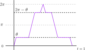
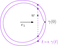
Figure 3. Proof of Theorem 12: Left: the graph of the function $g_{\theta,\beta}$, Right: the image of the loop $\gamma$ in the affine plane $P_{u}(w)$, the two circles visualise the round-trip of the loop.

The loop family.– Since $b$ induces a bijection between $]0,\pi[\times]0,1[$ and $D(\widetilde{r})$, there exists a unique couple $(\theta,\beta)\in\;]0,\pi[\times]0,1[$ such that $b(\theta,\beta)=w$. We define two functions $c_{1}$ and $c_{2}$ by the equality

$$c(\eta,\theta,\beta,\cdot)=(c_{1}(\cdot)+ic_{2}(\cdot),1)$$

($\eta$ will be chosen later). We put

$$\textbf{e}_{1}:=\widetilde{r}\frac{\nu}{\|\nu\|_{h}},\;\;\;\textbf{e}_{2}:=\widetilde{r}\frac{L(u)-\mbox{proj}_{P}L(u)}{\|L(u)-\mbox{proj}_{P}L(u)\|_{h}}\;\;\;\mbox{and}\;\;\;\textbf{e}_{3}:=\mbox{proj}_{P}L(u)$$

and we define the loop family $\gamma$$\blacksquare$ $\gamma$ by

$$\textstyle{\textup{\raisebox{1.7pt}{$\gamma$\raisebox{-6.5pt}{{\color[rgb]{1,1,1}$\blacksquare$}}} $\gamma$}}(\sigma,w)(t):=c_{1}(t)\textbf{e}_{1}+c_{2}(t)\textbf{e}_{2}+\textbf{e}_{3}.$$

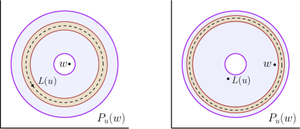
Figure 4. Proof of Theorem 12: In purple, the trace of the relation on $P_{u}(w)$, in black (dashed line) the boundary of disk $D(\widetilde{r})$ and in brown, the annulus $A(\tilde{r}(1-\eta),\tilde{r}(1+\eta))$ depending on whether $\sqrt{\|L(u)\|_{h}^{2}-\|\mbox{proj}_{P}L(u)\|_{h}^{2}}>\sqrt{\|w\|_{h}^{2}-\|\mbox{proj}_{P}w\|_{h}^{2}}+\frac{1}{3}d_{1}(w)$ (left) or not (right), see the definition of $\widetilde{r}$.

The image of the loop $\textstyle{\textup{\raisebox{1.7pt}{$\gamma$\raisebox{-6.5pt}{{\color[rgb]{1,1,1}$\blacksquare$}}} $\gamma$}}(\sigma,w)$ is the translated circle $\partial D(\tilde{r})+\tilde{r}\eta\cos\theta\textbf{e}_{1}$ which lies inside the annulus $A(\tilde{r}(1-\eta),\tilde{r}(1+\eta))$ of $P_{u}(w)$. Consequently, to ensure that the image of $\textstyle{\textup{\raisebox{1.7pt}{$\gamma$\raisebox{-6.5pt}{{\color[rgb]{1,1,1}$\blacksquare$}}} $\gamma$}}(\sigma,w)$ is in the relation, it is enough to choose $\eta$ such that $A(\tilde{r}(1-\eta),\tilde{r}(1+\eta))\subset A(r_{min}(\epsilon),r_{max}(\epsilon))=\mathcal{I\!\!s}(\epsilon)(\sigma,\lambda,u)\cap P_{u}(w)$. It is readily checked that the choice

$$\eta:=\frac{1}{3}\min(d_{1}(w),d_{2}(L(u)))$$

where $d_{2}(L(u))=dist(L(u),\partial A(r_{min}(\epsilon),r_{max}(\epsilon)))$ is convenient. It is also straightforward to see that this loop family satisfies the Average Constraint: $\overline{\textstyle{\textup{\raisebox{1.7pt}{$\gamma$\raisebox{-6.5pt}{{\color[rgb]{1,1,1}$\blacksquare$}}} $\gamma$}}}(\sigma,w)=w.$ The base point of the loop is $\textstyle{\textup{\raisebox{1.7pt}{$\gamma$\raisebox{-6.5pt}{{\color[rgb]{1,1,1}$\blacksquare$}}} $\gamma$}}(\sigma,w)(0)=(1+\eta\cos\theta)\textbf{e}_{1}+\textbf{e}_{3}$. The homotopy $H(s):=(\cos s\;\textbf{e}_{1}+\sin s\;\textbf{e}_{2})+\eta\cos\theta\textbf{e}_{1}+\textbf{e}_{3}$ with $s\in\;[0,\frac{\pi}{2}]$ connects $\textstyle{\textup{\raisebox{1.7pt}{$\gamma$\raisebox{-6.5pt}{{\color[rgb]{1,1,1}$\blacksquare$}}} $\gamma$}}(\sigma,w)(0)$ with $\eta\cos\theta\textbf{e}_{1}+\textbf{e}_{2}+\textbf{e}_{3}$ A linear homotopy joins this last point to $L(u)=(\|L(u)-\mbox{proj}_{P}L(u)\|_{h})\textbf{e}_{2}/\widetilde{r}+\textbf{e}_{3}.$ Consequently, the loop family $\gamma$$\blacksquare$ $\gamma$ is $c$-shaped and surrounding (see Definition 8). This proves that $\mathcal{I\!\!s}(\epsilon)$ is a Kuiper relation.

3. An application: desingularization of a cone to a surface $\epsilon$-isometric to a flat cylinder

Proposition 11 together with the Kuiper property of the relation of $\epsilon$-isometric maps are the reason of the absence of integrals in the formula proposed in [3, 1] to solve $\mathcal{I\!\!s}(\epsilon)$. The approach developed here also allows to apply the $h$-principle in its full generality for $\mathcal{I\!\!s}(\epsilon)$. Indeed, in the above cited references, the formulas only make sense when the base map $f_{0}$ is an immersion but in the framework of the $h$-principle this hypothesis is not required: provided that $\mathfrak{S}$ is a subsolution, any base map $f_{0}$, singular or not, is convenient.

Here, we illustrate this point with a basic example. We consider a singular map sending a flat cylinder onto a cone and we use the Kuiper property of $\mathcal{I\!\!s}(\epsilon)$ to build an $\epsilon$-isometric map arbitrarily closed (in the $C^{0}$ sense) to the initial singular map.

3.1. Formal solution

We identify the flat cylinder of height $\frac{1}{20}$ and radius $\frac{1}{2\pi}$ with the space $Cyl=\mathbb{R}/\mathbb{Z}\times[-10^{-1},10^{-1}]$ endowed with the Euclidean metric. We define our formal solution to be

$$\mathfrak{S}_{0}:(x,y)\longmapsto((x,y),f_{0}(x,y),v_{1}(x,y),\partial_{2}f_{0}(x,y))$$

where $f_{0}$ is a parametrization of a cone:

$$f_{0}(x,y)=\frac{1}{\sqrt{2}}\Big{(}y\cos(2\pi x),y\sin(2\pi x),y\Big{)}$$

and $v_{1}$ is such that $\partial_{1}f_{0}(x,y)=\sqrt{2}\pi yv_{1}(x,y)$. Precisely:

$$v_{1}(x,y)=\Big{(}-\sin(2\pi x),\cos(2\pi x),0\Big{)}.$$

Observe that for every $(x,y)$ we have

$$\left\{\begin{array}[]{l}\|v_{1}(x,y)\|=1\\ \|\partial_{2}f_{0}(x,y)\|=1\\ \langle v_{1}(x,y),\partial_{2}f_{0}(x,y)\rangle=0\end{array}\right.$$

so the section $\mathfrak{S}_{0}$ is a formal solution of the relation of $\epsilon$-isometric maps for every $\epsilon>0$.

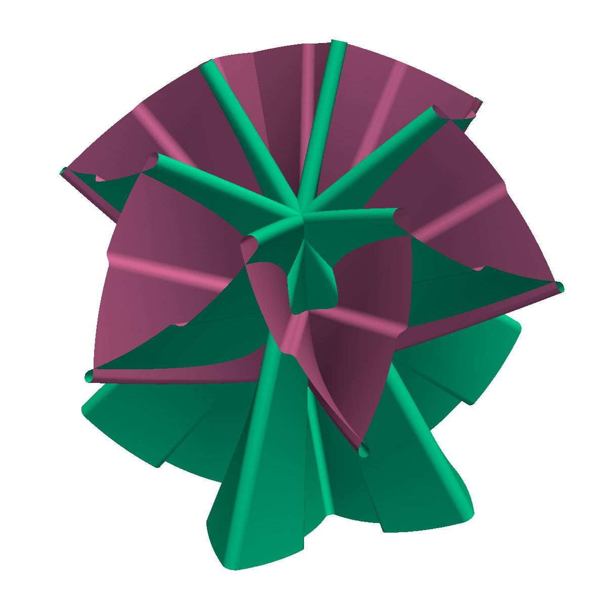
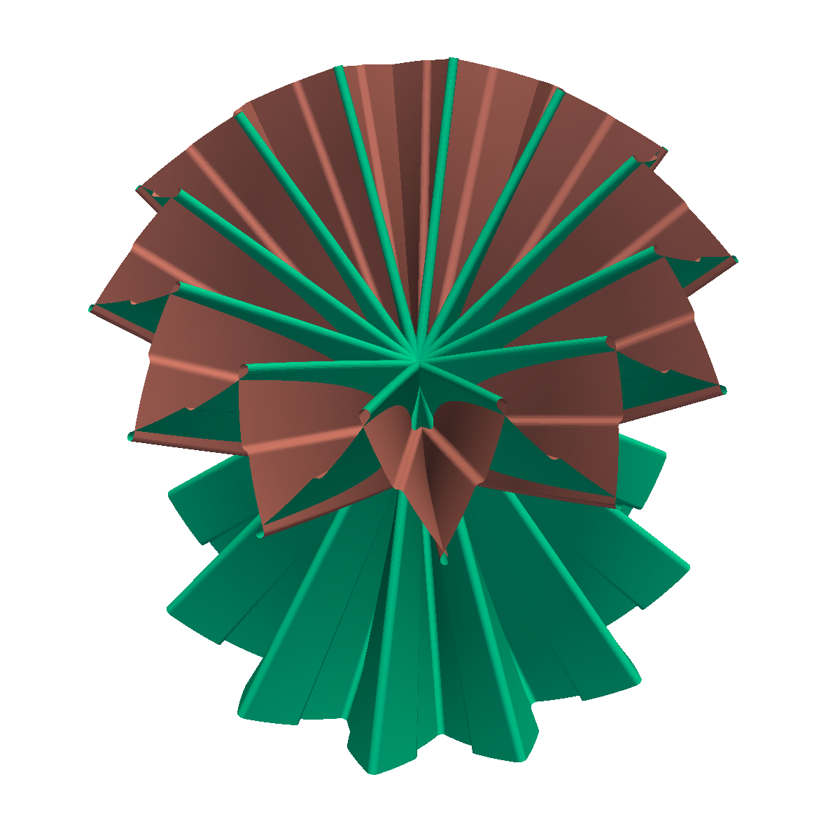
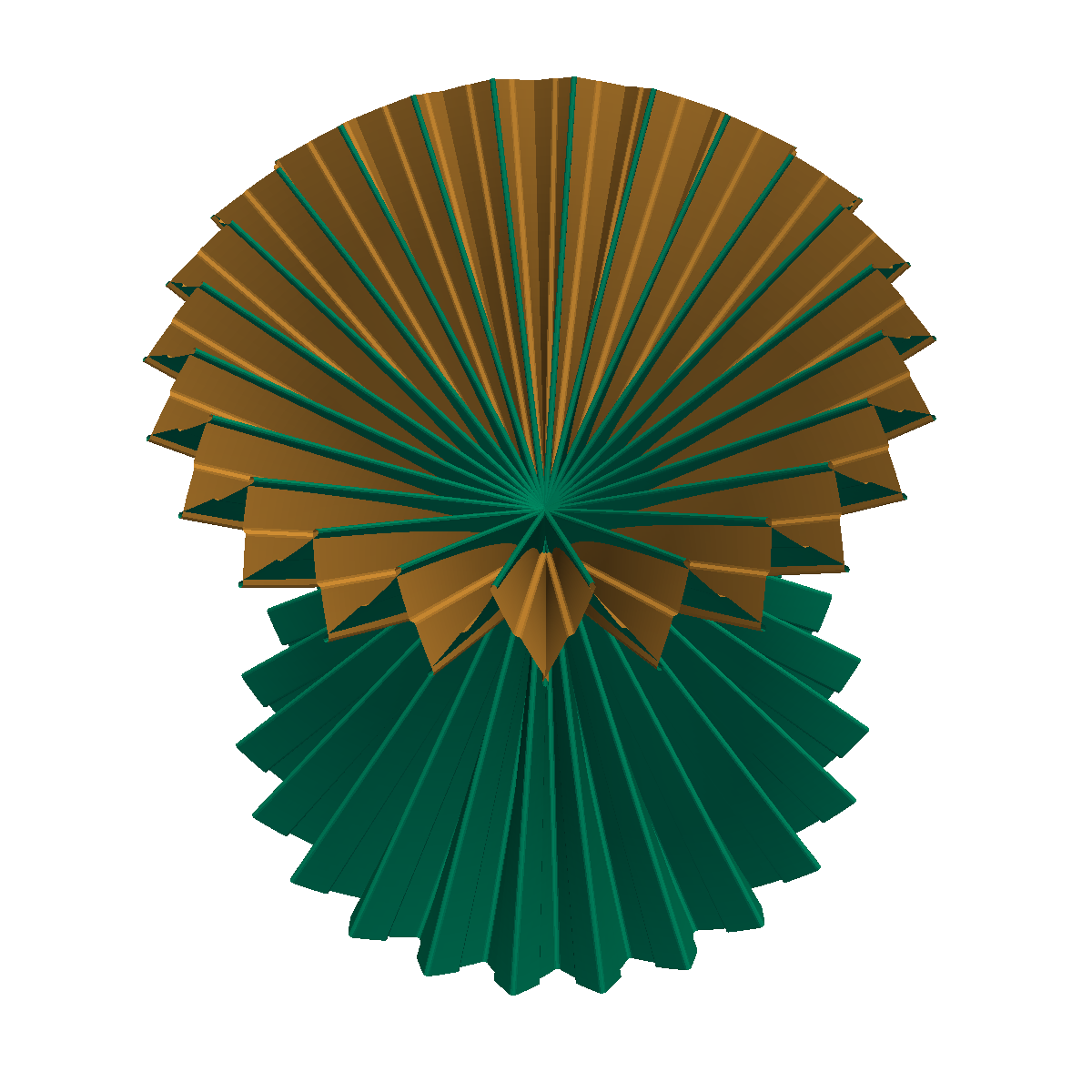
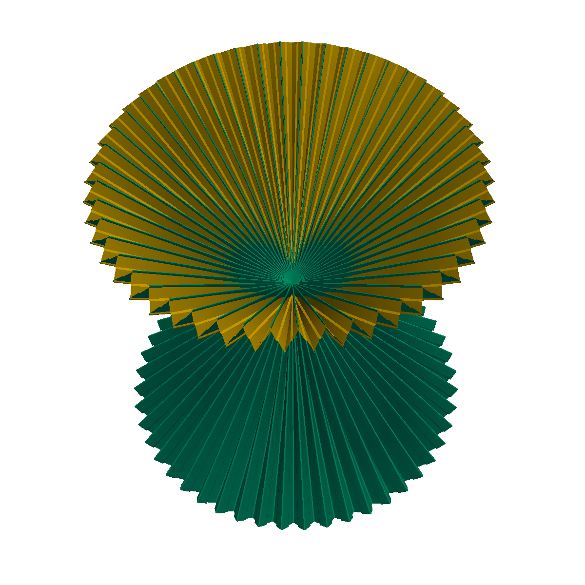
Figure 5. Corrugation Process applied from a cone: Several images of $f_{1}(Cyl)$ with $\eta=0.2$ and, from left to right and up to down, $N=6,12,24,48$. Observe the $C^{0}$-density property (see Proposition 4 $(P1)$) : the larger $N$, the closer the surface to the cone.

3.2. Subsolution

The section $\mathfrak{S}_{0}$ fails to be holonomic only in its $v_{1}$-component. To obtain a holonomic section, we thus intend to apply a Corrugation Process in the direction $\partial_{1}$. To do so, we need to check that $\mathfrak{S}_{0}$ is a subsolution with respect to $\partial_{1}$. As $v_{1}$ and $\partial_{2}f_{0}$ are orthogonal, the slice $\mathcal{I\!\!s}(\mathfrak{S}_{0},\partial_{1})$ lies inside the plane spanned by $v_{1}$ and the normal vector

$$n(x,y)=v_{1}(x,y)\wedge\partial_{2}f_{0}(x,y)=\frac{1}{\sqrt{2}}\Big{(}\cos(2\pi x),\sin(2\pi x),-1\Big{)}$$

(see the proof of Theorem 12). This slice is a circle of radius 1. The section $\mathfrak{S}_{0}$ is a subsolution if and only if the derivative $\partial_{1}f_{0}$ lies in the convex hull of $\mathcal{I\!\!s}(\mathfrak{S}_{0},\partial_{1})$. This condition is equivalent to $|y|<(\sqrt{2}\pi)^{-1}.$ Since $y\in[-10^{-1},10^{-1}]$, this last inequality is fulfilled. This shows that $\mathfrak{S}_{0}$ is subsolution with respect to $\partial_{1}$ of $\mathcal{I\!\!s}(\mathfrak{S}_{0},\partial_{1})$, and thus of $\mathcal{I\!\!s}(\epsilon)(\mathfrak{S}_{0},\partial_{1})$ for every $\epsilon>0.$

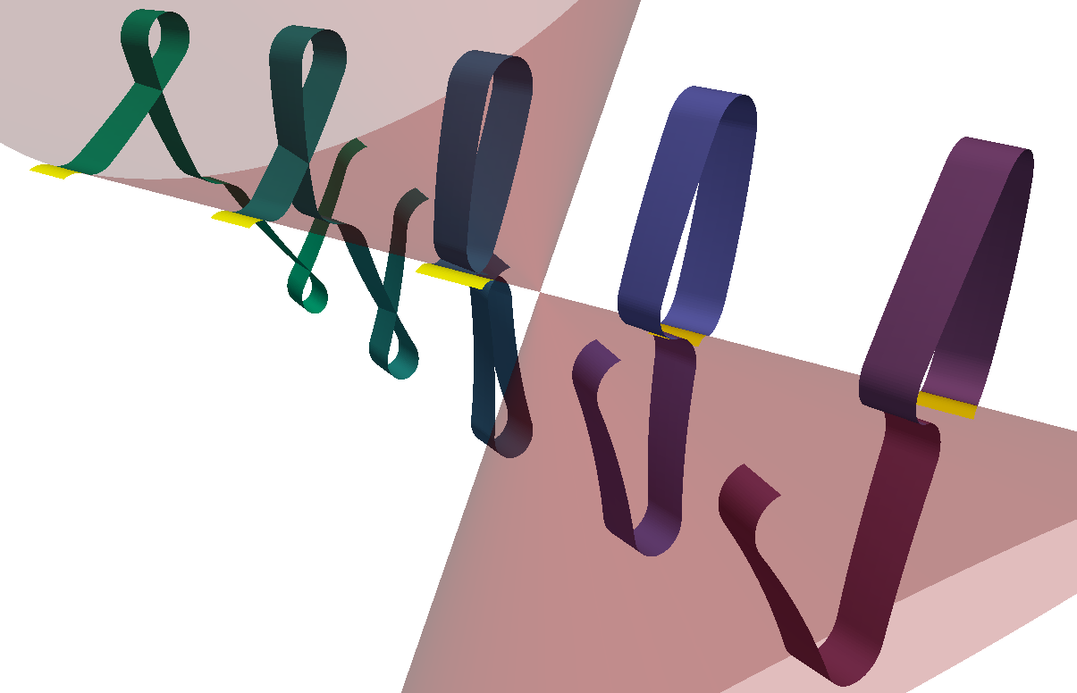
Figure 6. The change of the shape of a corrugation when passing the conical singularity.: Here $N=6$ and $\eta=0.4$.

Figure 7. Lengths and Corrugations: In blue, two slices of the image $f_{1}(Cyl)$ for $N=6$, in pink, two slices for $N=24$. On the right the slices are above the horizontal plane passing though the vertex of the cone. They are below this plane on the left. In all cases $\eta=0.2$.

3.3. Corrugation Process

We consider the shape $c:Cyl\times\mathbb{R}/\mathbb{Z}\rightarrow\mathbb{C}\times\mathbb{R}$ defined in subsection 12 where $\mathbb{C}$ is identified with the plane spanned by $(v_{1},n)$:

$$c(\eta,\theta,\beta,t):=(\exp(ig_{\theta,\beta}(t))+\eta\cos\theta,1).$$

In that expression, $\beta$ and $\theta$ are defined by the relation

$$\partial_{1}f_{0}=\beta e^{i\theta}+(1-\beta)e^{-i\theta}.$$

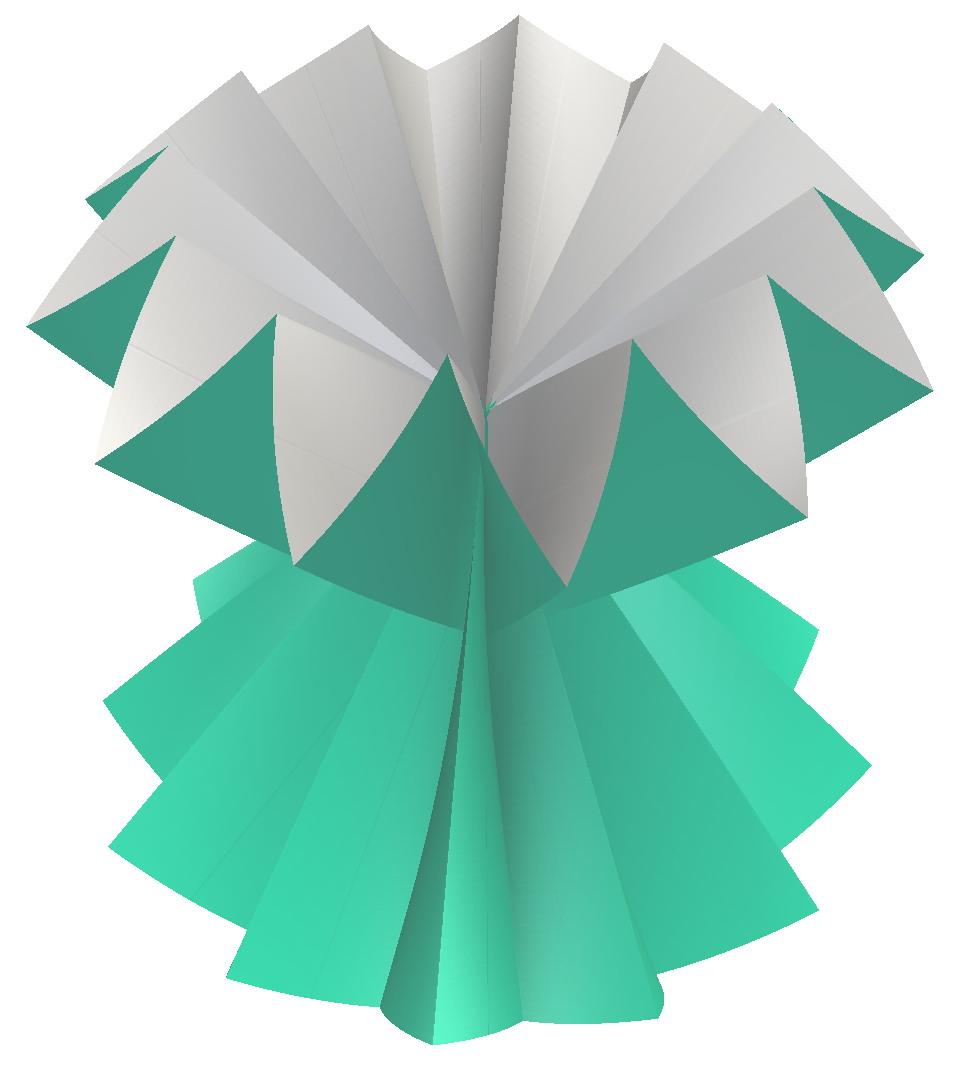
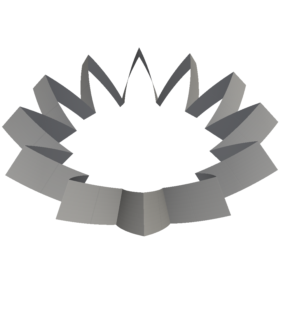
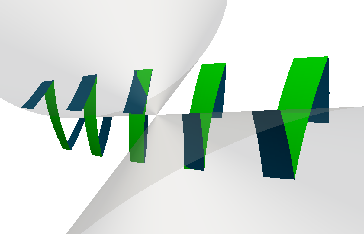
Figure 8. PL behavior: Here $\eta=10^{-3}$ and $N=12$. Despite appearances, the map $f_{1}$ is still a $C^{1}$-immersion. See the close up of Figure 9.

Since $v_{1}$ is collinear to $\partial_{1}f_{0}$ the coefficient $\beta$ is constant equal to $1/2$ and $\theta=\arccos(\langle\partial_{1}f_{0},v_{1}\rangle)=\arccos(\sqrt{2}\pi y)$. For short we denote $g$ for $g_{\theta,\beta}.$ The loop family $\gamma$ is thus given by

$$\gamma(x,y,t)=\Big{(}\cos(g(x,y,t))+\eta\|\partial_{1}f_{0}(x,y)\|\Big{)}v_{1}(x,y)+\sin(x,y,t)n(x,y).$$

Observe that $\gamma(x,y,t)\in\mathcal{I\!\!s}(\eta)(\mathfrak{S}_{0},\partial_{1})$. The Corrugation Process generates a map $f_{1}(x,y)=f_{0}(x,y)+\frac{1}{N}\Gamma(x,y,Nx)$ with

$$\Gamma(x,y,t):=\int_{s=0}^{t}\gamma(x,y,s)-\overline{\gamma(x,y)}ds.$$

Recall that, from Point $(P_{3})$ of Proposition 4, we have

$$\partial_{1}f_{1}(x,y)=\gamma(x,y,Nx)+O(1/N).$$

Let $\epsilon>0$ be given. To insure $\partial_{1}f_{1}\in\mathcal{I\!\!s}(\epsilon)(\mathfrak{S}_{0},\partial_{1})$ we have to choose $\eta<\epsilon$ and $N$ large enough.

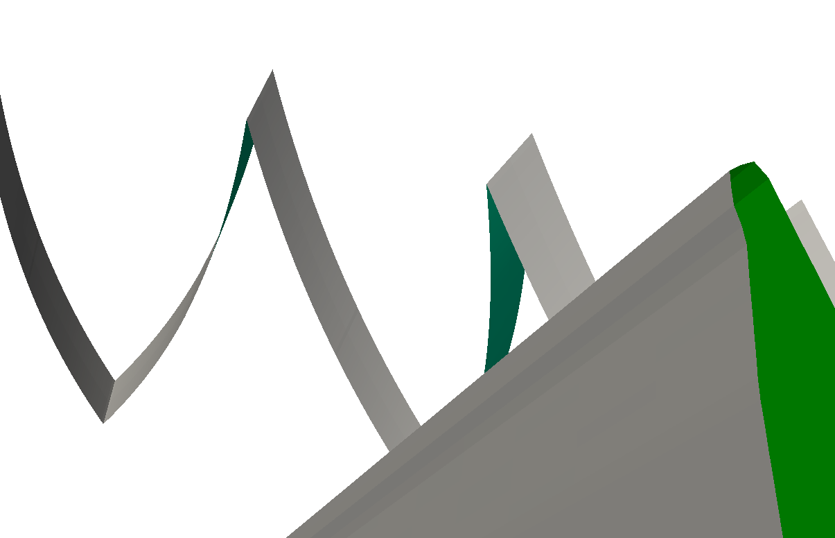
Figure 9. Zoom on the peak of a corrugation: The peak is not a folding. For $N$ large enough, the corrugations are immersed. A close-up shows the roundness of the peak (in the foreground). The angles that appear are artefact due to the discretisation step.

3.4. Numerical implementation

We use the analytical expression of Proposition 11 together with the above expression of $\gamma$ to implement the Corrugation Process. The images reveal corrugations whose shape varies from a small loop to the one of a roof. A closer look to the surface shows that the shape of the corrugations changes precisely when passing the vertex of the cone. The reason of this behavior is that $v_{1}$ the invariant by vertical translation (as opposed to the invariance by central symmetry of the cone and of $\partial_{1}f_{0}$). When $\eta$ decreases toward zero the map $g$ tends towards a piecewise constant map. Each loop in the family $\gamma$ stays at the two points $\cos\theta\,v_{1}\pm\sin\theta\,n$ for a duration of $\frac{1-\eta}{2}$ each. At the limit, $\gamma$ is a discontinuous map whose image is two points. As a consequence, when $\eta$ is small, the image $f_{1}(Cyl)$ looks like a piecewise linear surface.

References

- [1] S. Conti, C. De Lellis, and L. Székelyhidi, Jr. -principle and rigidity for isometric embeddings. In Nonlinear partial differential equations, volume 7 of Abel Symp., pages 83–116. Springer, Heidelberg, 2012.
- [2] M. Gromov. Partial differential relations. Springer-Verlag, Berlin, 1986.
- [3] N. Kuiper. On -isometric imbeddings. Indag. Math., volume 17:545–556, 1955.
- [4] J. Nash. isometric imbeddings. Ann. of Math., volume 60:383–396, 1954.
- [5] D. Spring. Convex integration theory, volume 92 of Monographs in Mathematics. Birkhäuser Verlag, Basel, 1998. Solutions to the -principle in geometry and topology.
- [6] M. Theillière. Convex integration without integration. ArXiv, 2019.