XOR Mixup: Privacy-Preserving Data Augmentation for One-Shot Federated Learning

Abstract

User-generated data distributions are often imbalanced across devices and labels, hampering the performance of federated learning (FL). To remedy to this non-independent and identically distributed (non-IID) data problem, in this work we develop a privacy-preserving XOR based mixup data augmentation technique, coined XorMixup, and thereby propose a novel one-shot FL framework, termed XorMixFL. The core idea is to collect other devices’ encoded data samples that are decoded only using each device’s own data samples. The decoding provides synthetic-but-realistic samples until inducing an IID dataset, used for model training. Both encoding and decoding procedures follow the bit-wise XOR operations that intentionally distort raw samples, thereby preserving data privacy. Simulation results corroborate that XorMixFL achieves up to $17.6$% higher accuracy than Vanilla FL under a non-IID MNIST dataset.

1 Introduction

Securing more data is essential in imbuing more intelligence into machine learning (ML) models. In view of this, the problem of utilizing the sheer amount of user-generated private data has attracted significant attention in both academia and industry (Park et al., 2019; Kairouz et al., 2019; Park et al., 2020). Federated learning (FL) is one promising solution based on exchanging model parameters among devices without sharing raw data, thereby preserving data privacy (McMahan et al., ; Konečný et al., ; Yang et al., 2019b; Li et al., 2020). While effective under independent and identically distributed (IID) data distributions, the performance of FL is highly degraded under non-IID user-generated data in practice (Zhao et al., 2018a; Oh et al., ). Indeed, when each device has scarce samples of specific labels, the classification accuracy under MINST and CIFAR-10 datasets is degraded by up to $11$% and $51$%, respectively, compared to the IID counterparts (Zhao et al., 2018b).

On this account, in this article we seek for an FL solution coping with non-IID data distributions. Inspired by the Mixup data augmentation technique (Vanilla Mixup) producing a synthetic sample by linearly superpositioning two raw samples (Zhang et al., 2018), we first propose an XOR based mixup data augmentation method (XorMixup) that is extended to a novel FL framework, termed XorMixFL.

Figure 1: A schematic illustration of XorMixFL in which XorMixup data augmentation is used for correcting non-IID data distributions while preserving raw data privacy.

XorMixup.

The key idea is to exploit the flipping property of the bit-wise XOR operation $\oplus$: $(A\oplus B)\oplus B=A$. For two devices $d_{1}$ and $d_{2}$, XorMixup is operated as follows.

1. $d_{1}$ generates an encoded seed sample $A\oplus B)$ by mixing samples $A$ and $B$ in different labels, transmitted to $d_{2}$.

2. $d_{2}$ decodes $(A\oplus B)$ by mixing $(A\oplus B)$ and its own sample $B^{\prime}$ having the same label of $B$, via $(A\oplus B)\oplus B^{\prime}$, producing a synthetic sample $A^{\prime}$ that is similar to but different from $A$.

While both (i) and (ii) preserve raw data privacy between two devices, (ii) improves the synthetic sample’s authenticity, increasing one-shot FL accuracy as detailed next.

XorMixFL.

As illustrated in Fig. 1, by applying XorMixup to a one-shot FL framework having only one communication round (Guha et al., ; Yoshida et al., 2019), each device in XorMixFL uploads its encoded seed samples to a server. The server decodes and augments the seed samples using its own base samples until all the samples are evenly distributed across labels. The server can be treated as one of the devices, or a parameter server storing an imbalanced dataset. Then, utilizing the reconstructed dataset, the server trains a global model that is downloaded by each device until convergence.

Contributions.

To the best of the authors’ knowledge, this is the first piece of FL research based on XOR operations for addressing the non-IID data problem. Under a non-IID MNIST dataset, simulation results corroborate that XorMixFL achieves up to $8.13$% and $17.6$% higher accuracy than standalone ML and Vanilla FL, respectively. For an ablation study, we additionally propose a baseline one-shot FL (MixFL) whose encoding follows from Vanilla Mixup while ignoring decoding. Compared to MixFL, XorMixFL achieves comparable accuracy while preserving more data privacy, i.e., higher dissimilarity between the augmented and original data samples measured using the multidimensional scaling (MDS) method (Cox & Cox, 2008), highlighting the importance of XorMixup in one-shot FL.

2 Related Work

Existing one-shot FL schemes (Guha et al., ; Yoshida et al., 2019) consider that each devices first trains a local model until convergence, and then the server constructs a global model by aggregating the converged local models. This does not take into consideration global data distributions, and is thus vulnerable to the non-IID data problem. By contrast, XorMixFL constructs the global model by training a model with synthetic samples that are uploaded from devices in one communication round while preserving their data privacy.

To preserve privacy while exchanging data samples, homomorphic encryption such as RSA (Gentry, 2009) or differential privacy mechanisms (Koda et al., ) can be used, with non-negligible computing overhead or accuracy degradation, respectively. Alternatively, XorMixup reduces the accuracy degradation with low complexity by leveraging Mixup data augmentation (Zhang et al., 2018) and XOR operations. The original purpose of Vanilla Mixup is oversampling. XorMixup additionally focuses on its privacy preserving benefit in that the combination distorts raw samples. Furthermore, instead of the linear combination used in Vanilla Mixup, we apply XOR operations that are often used in cipher algorithms for hiding original information (Churchhouse, 2001).

Several recent works also study FL frameworks based on data sample exchanges (Jeong et al., 2018, 2019; Oh et al., ). For one-shot FL under non-IID data, in (Jeong et al., 2018, 2019) a synthetic sample generator is trained after collecting seed samples, which may still violate data privacy. In (Oh et al., ), seed samples are collected after Vanilla Mixup encoding, for running knowledge distillation operations, rather than one-shot FL. For a comprehensive overview on data sample exchanges in the context of FL, compared to model parameter exchanges (McMahan et al., ; Konečný et al., ; Kim et al., ; Chen et al., 20019; Yang et al., 2019a; Wang et al., 2018; Amiri & Gunduz, 2019; Elgabli et al., 2020; Samarakoon et al., 2018; Chen et al., 2018) and model output exchanges (Jeong et al., 2018; Oh et al., ; Cha et al., ; Ahn et al., 2019, 2020), readers are encouraged to read (Park et al., 2018).

3 Methodology

In this section, we describes the system model under study and the operations of XorMixFL. Consider a one-shot FL system consisting of one server and $\mathcal{U}$ devices, as depicted in Fig. 1. The $i$-th device $u_{i}$ stores its local dataset $D_{i}$, where $i\in\{1,2,\dots,\mathcal{U}\}$. Let $c$ indicate the server training and distributing a global model after collecting samples from $\mathcal{U}$ devices in a privacy-preserving way.

In XorMixFL, the server $c$ aims to train a global model to classify unlabeled samples. We consider a supervised task with unlabeled features $x$ and their ground-truth labels $y$. All devices have the same label $y$, but store different features $x$. We assume that both devices and the server $c$ store their own datasets imbalanced across labels, i.e., a non-IID global dataset, in which some of the target labels are deficient in samples. For the $k$-th label, $c(k)$ denotes the number of samples in the server $c$. We hereafter refer to these samples as base samples that will be used for data augmentation to make the server’s training dataset balanced.

Before augmenting samples, the server $c$ informs its connected devices of its target labels lacking samples, and requests $q^{target}_{c,u_{i}}$ samples per target label to the device $u_{i}$. Then, the device uploads XOR encoded samples to the server $c$. At the server $c$, the encoded samples are decoded using XOR operations with the server’s base samples, generating a synthetic-but-realistic sample for correcting its imbalanced training dataset. The encoding preserves raw data privacy by mixing target-label samples and dummy-label (non-target-label) samples using the bit-wise XOR operations. Likewise, the decoding preserves data privacy by mixing the encoded sample not with the raw dummy sample but with the server $c$’s base sample.

After the decoding, due to the use of the server’s base samples, there exist residual noise, as shown in Fig. 1. This is partly intended to preserve privacy, but nonetheless too much noise is obviously harmful for accuracy. To avoid excessive noise, it is important to extract common feature before each encoding or decoding. To this end, up to $p$ samples within the same label are averaged as done in Vanilla Mixup (Zhang et al., 2018). This sample blending step not only extracts common features, but also preserves more privacy by mixing multiple samples. The aforementioned operations of XorMixFL are elaborated in the following three steps.

Table 1: List of Notations

Notation	Meaning
$\mathcal{U}$	# of devices
$u_{i}$	$i$-th device
$D_{i}$	Dataset of $u_{i}$
$c$	Server
$c(k)$	# of base samples in the $k$-th label at $c$
$p$	Maximum # of blending samples per label
$N$	# of target labels
$M$	# of dummy labels
$n$	# of samples per each target label
$m$	# of samples in the remaining M dummy labels
$q^{target}_{c}$	Total required # of samples at $c$
$q^{target}_{c,u_{i}}$	# of samples uploaded to $c$ from $u_{i}$
$x^{target}_{(u_{i},t)}$	Raw sample of a target label at $u_{i}$
$x^{dummy}_{(u_{i},t)}$	Raw sample of a dummy label at $u_{i}$
$x^{dummy}_{(c,t)}$	Base sample of a dummy label at $c$
$X^{enc}_{(u_{i},c)}$	Encoded sample at $u_{i}$, transmitted to $c$
$X^{dec}_{(c)}$	Decoded sample from $X^{enc}_{(u_{i},c)}$ at $c$

1) Sample Blending.

Let $x_{(u_{i},t)}^{target}$ denote an 1-dimensional vector whose elements are the target labels of device $u_{i}$ that the server wants to successfully receive. Let $x_{(u_{i},t)}^{dummy}$ represent an 1-dimensional vector whose label is not the target one. Per each label, up to $p$ samples are averaged, resulting in $g^{p}(x^{target}_{(u_{i},0)})$ and $g^{p}(x^{dummy}_{(u_{i},0)})$ for target and dummy labels, respectively. Here, $g^{p}(\cdot)$ is given by iteratively applying a sample blending function $g(x_{(u_{i},t)})$ by $p$ times, which is defined as

$$g(x_{(u_{i},t)})=\alpha x_{(u_{i},t)}+(1-\alpha)x_{(u_{i},t+1)},$$ (1)

where $\alpha\in(0,1)$ denotes the blending ratio of two samples.

2) XOR Encoding.

For given blended samples $g^{p}(x^{target}_{(u_{i},0)})$ and $g^{p}(x^{dummy}_{(u_{i},0)})$, we apply the bit-wise XOR operation, and obtain an encoded sample $X^{enc}_{(u_{i},c)}$, i.e.,

$$X^{enc}_{(u_{i},c)}=g^{p}(x^{target}_{(u_{i},0)})\oplus g^{p}(x^{dummy}_{(u_{i},0)}).$$ (2)

The encoded sample $X^{enc}_{(u_{i},c)}$ is sent from device $u_{i}$ to the server $c$.

3) XOR Decoding.

The server $c$ performs the sample blending operations with its own samples to yield $g^{p}(x^{dummy}_{(c,0)})$. Given $g^{p}(x^{dummy}_{(c,0)})$ and the XOR encoded sample $X^{enc}_{(u_{i},c)}$ received from $u_{i}$, the server $c$ applies the bit-wise XOR operation, resulting in the decoded sample $X^{dec}_{(c,u_{i})}$, given as

$$X^{dec}_{(c,u_{i})}=X^{enc}_{(u_{i},c)}\oplus g^{p}(x^{dummy}_{(c,0)}).$$ (3)

Note that $X^{dec}_{(c,u_{i})}$ is decoded not using the device $u_{i}$’s $g^{p}(x^{dummy}_{(u_{i},0)})$ in Eq. 2 but using the server’s own $g^{p}(x^{dummy}_{(c,0)})$ in Eq. 3, thereby preserving the privacy of the raw samples.

To illustrate, as visualized in Fig. 1, consider an example where a server lacking the samples of the target label $5$ out of 10 labels (digits $0,1,\dots,8,9$). To preserve the sample privacy, device 1 selects a dummy label $2$ at random, within which $p=2$ samples are blended. Likewise, device 1 performs the same operations for the target label $5$. Then, using XOR, device 1 encodes two blended samples $\{2\}$ and $\{5\}$ (see Eq. 2), and sends the encoded sample $\{2\oplus 5\}$ to the server. Next, to decode the received sample $\{2\oplus 5\}$, the server first blends its own samples in the dummy label 2, creating a dummy sample $\{2^{\prime}\}$. Then, the server applies XOR to $\{2\oplus 5\}$ and $\{2^{\prime}\}$, yielding the decoded sample $\{5^{\prime}\}$ (see Eq. 3). Finally, the server adds $\{5^{\prime}\}$ into its dataset, and then trains an ML model that is distributed to every device after the training completion.

Generalizing this to multiple samples, the server requests $q^{target}_{c,u_{i}}$ encoded samples to its connected device $u_{i}$. These operations of each device and the server are summarized by Algorithms 1 and 2, respectively.

Algorithm 1 Device’s XOR encoding procedure

  Input: target label, dummy label, $p$, and $q^{target}_{c,u_{i}}$

  repeat

    Randomly select a target-label sample $x^{target}_{(u_{i},0)}$

    Randomly select a dummy-label sample $x^{dummy}_{(u_{i},0)}$

    Blend $x^{target}_{(u_{i},0)}$ via Eq. 1 up to $p$ times, yielding $g^{p}\!(x^{target}_{(u_{i},0)})$

    Blend $\!x^{dummy}_{(u_{i},0)}\!$ via Eq. 1 up to $p$ times, yielding $g^{p}\!(x^{dummy}_{(u_{i},0)})$

    XOR the blended samples via Eq. 2, yielding $X^{enc}_{(u_{i},c)}$

    Store $X^{enc}_{(u_{i},c)}$ in a buffer

  until The buffer size = $q^{target}_{c,u_{i}}$

  Upload the buffer $\{X^{enc}_{(u_{i},c)}\}$ to the server $c$

4 Experiments

In this section, we numerically analyze the performance of the proposed XorMixFL scheme in a non-IID MNIST classification task. For the benchmark scheme, we consider standalone ML, Vanilla FL, and MixFL. Unless otherwise specified, by default we consider $U=3$ devices having $n=10$ samples per each target label while storing $m=200$ samples in the remaining $M$ dummy labels.

4.1 Accuracy Evaluation under Non-IID Data Distributions

In this subsection, we investigate the test accuracy and per-label accuracy of XorMixFL and its benchmark schemes, for a different $N\in\{1,2,4\}$. With $N=1$, Tab. 2 shows that XorMixFL achieves about 10% higher test accuracy than the standalone ML regardless of the choice of the target label. Compared to MixFL, XorMixFL shows around 2% lower test accuracy. This is because the augmented samples generated by XorMixup include more non-trivial noise to preserver more privacy than Vanilla Mixup used in MixFL, as visualized in Fig. 2. For each target-label accuracy, Fig. 3(a) shows that XorMixFL achievs 65% target-label accuracy that is 1.87x higher than standalone ML. This highlights the effectiveness of XorMiup in (one-shot) FL.

Next, with $N=2$, Tab. 2 illustrates that the test accuracy is slightly decreased from the cases with $N=1$, while still exhibiting a similar trend across the proposed and benchmark schemes. To be more specific, comparing Fig. 3(a) and (b), target-label accuracy also decreases with $N$, among which the label $0$ is relatively robust against $N$ while the label $4$ is sensitive to $N$. Indeed, the label $4$ accuracy is decreased by around $30$% compared to the case with $N=1$.

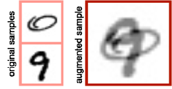
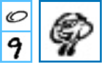
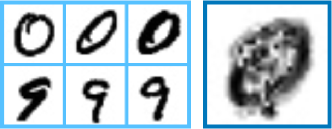
(a) Vanila Mixup.	(b) XorMixup, $p=1$	(c) XorMixup, $p=3$.

Figure 2: A visualization of original samples (target label: $0$, dummy label: $9$) and augmented samples using: (a) Vanilla Mixup, (b) XorMixup without sample blending ($p=1$), and (c) XorMixup with sample blending ($p=3$).

Method	1 Target Label, $N=1$										$N=2$				$N=4$
	0	1	2	3	4	5	6	7	8	9	(0, 2)	(0, 8)	(2, 4)	(4, 8)	($0,\!2,\!4,\!8$)
XorMixFL	94.44%	95.83%	95.28%	93.99%	94.72%	94.17%	94.58%	93.43%	94.65%	91.54%	92.36%	91.03%	92.61%	91.28%	88.48%
MixFL	96.85%	96.72%	95.59%	96.13%	95.82%	95.89%	95.52%	95.57%	95.56%	95.34%	95.52%	93.98%	94.87%	93.76%	91.93%
Vanilla FL	83.27%	84.83%	84.25%	83.49%	84.82%	83.82%	85.12%	83.31%	84.26%	82.94%	81.72%	81.23%	78.75%	79.23%	77.12%
Standalone	89.12%	88.62%	89.34%	91.13%	89.83%	88.31%	89.28%	90.11%	91.22%	87.43%	86.41%	88.16%	87.19%	86.58%	84.82%

Table 2: Test accuracy evaluation for different $N\in\{1,2,4\}$ ($p=1$, $\alpha=0.5$).

(a) 1 target label ($N=1$)	(b) 2 target labels ($N=2$)	(c) 4 target labels ($N=4$)

Figure 3: Target-label accuracy evaluation for different $N\in\{1,2,4\}$ $\alpha=0.5$: (a) $N=1$, where the blue, red, yellow bars represent XorMixFL, MixFL, and standalone ML, respectively; (b) $N=2$ (target labels: two of among 0, 2, 4, 8); and (c) $N=4$ (target labels: 0, 2, 4, 8). Tot denotes the test accuracy (averaged over all labels).

Lastly, with $N=4$, following the same tendency, Tab. 2 shows that test accuracy further decreases from $N=2$, and the resultant lowest test accuracy is $88.48$%. Likewise, as observed in Fig. 3(c), the target-label accuracy is also the lowest among the cases $N=1$, $2$, and $4$. Specifically, compared to the case with $N=2$ in Fig. 3(b), the target-label accuracy is decreased by around $4$%.

4.2 Data Privacy Evaluation

In this subsection, we study the sample privacy guarantee of the augmented dataset. Following (Jeong et al., 2019; Oh et al., ), the sample privacy is measured using the minimum MDS value (Cox & Cox, 2008) between the augmented sample and any raw sample contributing to the augmented sample. A larger MDS value implies higher dissimilarity, preserving more privacy.

Tab. 3 shows the MDS values of XorMixFL and MixFL with $N=1$. For the blending ratio $\alpha$, it is trivial that $\alpha$ biased towards either $0$ or $1$ more reveals one of the raw samples, while equal blending ($\alpha=0.5$) minimizes the raw sample leakage. Therefore, for MixFL that shows the highest accuracy in Sec. 4.1, we aim to preserve more privacy by choosing $\alpha=0.5$. By contrast, for XorMixFL, we aim to increase accuracy by choosing $\alpha=0.95$.

Algorithm 2 Server’s XOR decoding and training procedures

  Input: $\{X^{enc}_{(u_{i},c)}\}$, target label, dummy label, $p$, and $q^{target}_{c}$

  Inform connected devices of $q^{target}_{c,u_{i}}$ and target label

  repeat

    Randomly select a dummy-label sample $x^{dummy}_{(c,0)}$

    Blend $x^{dummy}_{(c,0)}$ via Eq. 2 up to $p$ times, yielding $g^{p}(x^{dummy}_{(c,0)})$

    XOR $X^{enc}_{(u_{i},c)}$ and $g^{p}(x^{dummy}_{(c,0)})$ via Eq. 3, yielding $X^{dec}_{(c,u_{i})}$

    Store $X^{dec}_{(c,u_{i})}$ in the training dataset

  until # of decoded samples = $q^{target}_{c}$

  Train the server’s model

  Broadcast the server’s trained model to all devices

As shown in Tab. 3, the value of MDS increases with the number $p$ of belnding samples and the number $M$ of dummy labels. Therefore, the lowest mean value of MDS in all cases of XorMixFL is $2116.96$, which is even higher than the maximum MDS value $2095.57$ of all cases in MixFL. The highest mean MDS value in XorMixFL is $3030.43$ when $M=3$ and $p=5$. The highest value of the MDS of MixFL is $2095.57$. The highest MDS value of XorMixFL is about 50% higher than that of MixFL. This results show that XorMixFL achieves preserves more data privacy than MixFL.

4.3 Impacts of Hyperparameters

In this subsection, we compare XorMixFL and MixFL in terms of the test accuracy and sensitivity to key design parameters: the number $M$ of dummy labels, sample blending weight $\alpha$, and the maximum number $p$ of blending samples per label. For all the parameter changes, XorMixFL is more robust against MixFL as elaborated next.

Test Accuracy.

First, we study the impact of $M$ on test accuracy. With $M=2$ under $p=1$ and $\alpha=0.25$, XorMixFL achieves the 95.29% test accuracy. With $M=3$, the test accuracy of XorMixFL is 91.60%. There is only 3.8% reduction in test accuracy, which is the largest reduction of XorMixFL when only the number of dummy labels changes. On the other hand, the test accuracy of MixFL is 94.49% when $M=1$ under $p=5$ and $\alpha=0.25$. With $M=3$, the test accuracy of MixFL drops to 85.65%, corresponding to 9.3% reduction. This is the largest reduction in MixFL when only the number of dummy labels changes.

Second, we investigate the impact of $\alpha$ on test accuracy. With $p=5$ under $M=2$ and $\alpha=0.5$, the test accuracy of XorMixFL is 92.78%. With $\alpha=0.25$, the test accuracy increases by around 2%. This is the largest increase in the test accuracy of XorMixFL. With $\alpha=0.95$, the test accuracy increases by around 5%. This is the largest increase in the test accuracy of MixFL.

Lastly, we consider the impact of $p$ on test accuracy. When $p=5$ under $\alpha=0.5$ and $M=2$, 92.78% is the test accuracy of XorMixFL. With $p=1$, the test accuracy increases by about 3%. However, With $p=5$ under $\alpha=0.95$ and $M=1$, the test accuracy of MixFL is 90.74%. When $p=1$, the test accuracy increases by about 5%.

		Number of Averaging Samples ($p$)
		$p=1$	2	3	4	5
XorMixFL	$M=1$	2116.97 / 335.85	2335.78 / 545.64	2520.88 / 687.77	2674.01 / 778.90	2781.09 / 838.49
	$M=2$	2321.38/ 352.65	2409.72 / 643.56	2664.12 / 814.13	2821.37 / 900.01	2911.42 / 947.06
	$M=3$	2406.62 / 365.61	2519.44 / 741.04	2800.24 / 895.33	2949.51 / 966.04	3030.43 / 1001.48
MixFL	$M=1$	1248.46 / 156.20	1342.34 / 213.23	1382.11 / 311.44	1402.53 / 292.41	1496.32 / 349.25
	$M=2$	1462.75 / 251.78	1523.10 / 320.13	1611.42 / 343.13	1683.45 / 391.39	1820.43 / 385.32
	$M=3$	1521.13 / 225.39	1621.47 / 276.52	1850.32 / 403.72	1999.01 / 545.66	2095.57 / 634.79

Table 3: MDS comparison (mean / standard deviation) between XorMixFL and MixFL (target label: $9$, $\alpha=0.5$).

			1 dummy label, $M=1$			2 dummy labels, $M=2$			3 dummy labels, $M=3$
			$\alpha$ = 0.25	0.5	0.95	0.25	0.5	0.95	0.25	0.5	0.95
XorMixFL	$p$ = 1	Test Acc.	92.33%	92.54%	92.05%	95.29%	95.10%	94.47%	91.60%	91.51%	90.82%
		Per-label Acc.	52.89%	54.48%	51.65%	80.01%	77.61%	74.45%	44.62%	41.98%	39.72%
	$p$ = 5	Test Acc.	91.75%	92.98%	93.11%	94.37%	92.78%	94.19%	90.82%	90.42%	91.60%
		Per-label Acc.	46.16%	56.55%	60.28%	69.59%	56.23%	68.95%	34.92%	33.42%	43.68%
MixFL	$p$ = 1	Test Acc.	94.49%	94.49%	95.96%	87.85%	90.65%	91.98%	87.44%	90.31%	91.86%
		Per-label Acc.	72.82%	72.60%	72.73%	21.94%	43.36%	47.72%	19.78%	40.91%	46.46%
	$p$ = 5	Test Acc.	94.49%	90.07%	90.74%	88.64%	86.21%	90.71%	85.65%	86.03%	90.66%
		Per-label Acc.	42.08%	32.82%	35.67%	26.83%	24.71%	34.76%	15.42%	24.30%	34.72%

Table 4: The average test accuracy of XorMixFL and MixFL when the number of dummy label and the value of $\alpha$ for image blending procedure changes (target label: $9$, dummy labels: $3$ and/or $4$ and/or $5$).

Target-Label Accuracy.

In terms of per-label accuracy, we compare the impact of $M$ and $\alpha$. First, when $\alpha=0.5$ under $p=1$, and three dummy labels are used, the per-label accuracy of XorMixFL is 41.98%. When $M=2$, the per-label accuracy increase by about 84%, leading to the per-label accuracy 77.61%. This is the largest percent change in XorMixFL when only the number of dummy labels changes. On the other hand, when $\alpha=0.25$ under $p=1$ and $M=3$, the per-label accuracy of MixFL is 19.78%. When $M=1$, the per-label accuracy increase by about 268%, resulting in the per-label accuracy 72.82%. This is the largest percent change in MixFL when only the number of dummy labels changes.

Second, we study the impact of the blending weight $\alpha$ on the per-label accuracy. When $p=5$ under $\alpha=0.25$ and $M=1$, the per-label accuracy of XorMixFL is 46.16%. When $\alpha=0.95$, the per-label accuracy increase by about 30%, resulting in the per-label accuracy is 60.28%. This is the largest increase in the per-label accuracy of XorMixFL when only $\alpha$ changes. On the other hand, when $p=1$ under $\alpha=0.25$ and $M=3$, the per-label accuracy of MixFL is 19.78%. When $\alpha=0.95$, the per-label accuracy increases by about 134%, leading to the per-label accuracy 46.46%.

Lastly, we investigate the impact of $p$ on the per-label accuracy. With $p=5$ under $\alpha=0.5$ and $M=2$, the per-label accuracy of XorMixFL is 56.23%. The per-label accuracy increases by about 38% when $p=1$, yielding the per-label accuracy 77.61% of XorMixFL. However, with $p=5$ under $\alpha=0.25$ and $M=1$, the per-label accuracy of MixFL is 42.08%. With $p=1$, the per-label accuracy increases by about 73%, achieving 72.82% per-label accuracy of MixFL.

5 Conclusion

In this work, we proposed a novel privacy-preserving one-shot FL framework, XorMixFL, which allows devices to locally augment insufficient samples to correct the non-IID data distributions while hiding the details of the original samples. Numerical simulations validate the effectiveness of XorMixFL in terms of accuracy and privacy guarantees, while discovering the impacts of key design parameters such as the numbers of blending samples and dummy labels on accuracy and privacy guarantees. Exploiting the core idea, XorMixup data augmentation, it could be interesting to extend our one-shot FL framework to the standard multi-shot FL applications for future study.

References

- Ahn et al. (2019) Ahn, J., Simeone, O., and Kang, J. Wireless federated distillation for distributed edge learning with heterogeneous data. IEEE International Symposium on Personal, Indoor and Mobile Radio Communications (PIMRC), Istanbul, Turkey, Sep. 2019.
- Ahn et al. (2020) Ahn, J., Simeone, O., and Kang, J. Cooperative learning via federated distillation over fading channels. in Proc. IEEE International Conference on Acoustics, Speech and Signal Processing (ICASSP), Barcelona, Spain, May 2020.
- Amiri & Gunduz (2019) Amiri, M. M. and Gunduz, D. Over-the-air machine learning at the wireless edge. Proc. IEEE International Workshop on Signal Processing Advances in Wireless Communications (SPWAC), Cannes, France, July 2019.
- (4) Cha, H., Park, J., Kim, H., Bennis, M., and Kim, S.-L. Federated reinforcement distillation with proxy experience replay memory. to appear in IEEE Intelligent Systems.
- Chen et al. (20019) Chen, M., Yang, Z., Saad, W., Yin, C., Poor, H. V., and Cui, S. A joint learning and communications framework for federated learning over wireless networks. arXiv preprint arXiv: 1909.07972, 20019.
- Chen et al. (2018) Chen, T., Giannakis, G., Sun, T., and Yin, W. Lag: Lazily aggregated gradient for communication-efficient distributed learning. In Advances in Neural Information Processing Systems, pp. 5055–5065, 2018.
- Churchhouse (2001) Churchhouse, R. F. Codes and Ciphers: Julius Caesar, the Enigma, and the Internet. Cambridge University Press, 2001.
- Cox & Cox (2008) Cox, M. A. A. and Cox, T. F. Multidimensional Scaling. Springer Berlin Heidelberg, Berlin, Heidelberg, 2008.
- Elgabli et al. (2020) Elgabli, A., Park, J., Bedi, A. S., Bennis, M., and Aggarwal, V. GADMM: Fast and communication efficient framework for distributed machine learning. Journal of Machine Learning Research (JMLR), 21(76):1–39, 2020.
- Gentry (2009) Gentry, C. Fully homomorphic encryption using ideal lattices. in Proc. ACM Symposium on Theory of Computing, Bethesda, MD, USA, pp. 169–178, 2009.
- (11) Guha, N., Talwalkar, A., and Smith, V. One-shot federated learning. [Online]. Arxiv preprint: http://arxiv.org/abs/1902.11175.
- Jeong et al. (2018) Jeong, E., Oh, S., Kim, H., Park, J., Bennis, M., and Kim, S.-L. Communication-efficient on-device machine learning: Federated distillation and augmentation under non-iid private data. presented at Neural Information Processing Systems Workshop on Machine Learning on the Phone and other Consumer Devices (MLPCD), Montréal, Canada, 2018. doi: arXiv:1811.11479. URL http://arxiv.org/abs/1811.11479.
- Jeong et al. (2019) Jeong, E., Oh, S., Park, J., Kim, H., Bennis, B., and Kim, S.-L. Multi-hop federated private data augmentation with sample compression. presented at International Joint Conference on Artificial Intelligence (IJCAI) Wksp. Federated Machine Learning for User Privacy and Data Confidentiality (FML), Macau, China, Aug. 2019.
- Kairouz et al. (2019) Kairouz, P., McMahan, H. B., Avent, B., Bellet, A., Bennis, M., Bhagoji, A. N., Bonawitz, K., Charles, Z., Cormode, G., Cummings, R., et al. Advances and open problems in federated learning. arXiv preprint arXiv:1912.04977, 2019.
- (15) Kim, H., Park, J., Bennis, M., and Kim, S.-L. Blockchained on-device federated learning. to appear in IEEE Communications Letters [Online]. ArXiv preprint: abs/1808.03949.
- (16) Koda, Y., Yamamoto, K., Nishio, T., and Morikura, M. Differentially private aircomp federated learning with power adaptation harnessing receiver noise. [Online]. Arxiv preprint: https://arxiv.org/abs/2004.06337.
- (17) Konečný, J., McMahan, H. B., Ramage, D., and Richtárik, P. Federated Optimization: Distributed Machine Learning for On-Device Intelligence. [Online]. Available: http://arxiv.org/abs/1610.02527. URL http://arxiv.org/abs/1610.02527.
- Li et al. (2020) Li, T., Sahu, A. K., Talwalkar, A., and Smith, V. Federated learning: Challenges, methods, and future directions. IEEE Signal Processing Magazine, 37(3):50–60, May 2020.
- (19) McMahan, H. B., Moore, E., Ramage, D., Hampson, S., and Arcas, B. A. y. Communication-Efficient Learning of Deep Networks from Decentralized Data. In Proc. AISTATS, Fort Lauderdale, FL, USA. Apr. 2017.
- (20) Oh, S., Park, J., Jeong, E., , Kim, H., Bennis, M., and Kim, S.-L. Mix2FLD: Downlink federated learning after uplink federated distillation with two-way mixup. to appear in IEEE Communications Letters.
- Park et al. (2018) Park, J., Wang, S., Elgabli, A., Oh, S., Jeong, E., Cha, H., Kim, H., Kim, S.-L., and Bennis, M. Distilling on-device intelligence at the network edge. [Online]. Arxiv preprint: http://arxiv.org/abs/1907.02745, December 2018.
- Park et al. (2019) Park, J., Samarakoon, S., Bennis, M., and Debbah, M. Wireless network intelligence at the edge. Proceedings of the IEEE, 107(11):2204–2239, October 2019.
- Park et al. (2020) Park, J., Samarakoon, S., Shiri, H., Abdel-Aziz, M. K., Nishio, T., Elgabli, A., and Bennis, M. Extreme URLLC: Vision, challenges, and key enablers. arXiv preprint arXiv:2001.09683, 2020.
- Samarakoon et al. (2018) Samarakoon, S., Bennis, M., Saad, W., and Debbah, M. Federated learning for ultra-reliable low-latency v2v communications. In 2018 IEEE Global Communications Conference (GLOBECOM), pp. 1–7. IEEE, 2018.
- Wang et al. (2018) Wang, S., Tuor, T., Salonidis, T., Leung, K. K., Makaya, C., He, T., and Chan, K. Adaptive federated learning in resource constrained edge computing systems. ArXiv preprint, abs/1804.05271, 2018.
- Yang et al. (2019a) Yang, H. H., Liu, Z., Quek, T. Q. S., and Poor, H. V. Scheduling policies for federated learning in wireless networks. arXiv preprint arXiv: 1908.06287, 2019a.
- Yang et al. (2019b) Yang, Q., Liu, Y., Chen, T., and Tong, Y. Federated machine learning: Concept and applications. ACM Transactions on Intelligent Systems and Technology, 10(2), Feb. 2019b.
- Yoshida et al. (2019) Yoshida, N., Nishio, T., Morikura, M., Yamamoto, K., and Yonetani, R. Hybrid-fl: Cooperative learning mechanism using non-iid data in wireless networks. arXiv preprint arXiv:1905.07210, 2019.
- Zhang et al. (2018) Zhang, H., Cisse, M., Dauphin, Y. N., and Lopez-Paz, D. mixup: Beyond Empirical Risk Minimization. In Proc. of 6th International Conference on Learning Representations (ICLR), 2018.
- Zhao et al. (2018a) Zhao, Y., Li, M., Lai, L., Suda, N., Civin, D., and Chandra, V. Federated Learning with Non-IID Data. [Online]: arXiv preprint arXiv:1806.00582, 2018a. URL http://arxiv.org/abs/1806.00582.
- Zhao et al. (2018b) Zhao, Y., Li, M., Lai, L., Suda, N., Civin, D., and Chandra, V. Federated learning with non-iid data. arXiv preprint arXiv:1806.00582, 2018b.