Matrix games with bandit feedback

Abstract

We study a version of the classical zero-sum matrix game with unknown payoff matrix and bandit feedback, where the players only observe each others actions and a noisy payoff. This generalizes the usual matrix game, where the payoff matrix is known to the players. Despite numerous applications, this problem has received relatively little attention. Although adversarial bandit algorithms achieve low regret, they do not exploit the matrix structure and perform poorly relative to the new algorithms. The main contributions are regret analyses of variants of UCB and K-learning that hold for any opponent, e.g., even when the opponent adversarially plays the best-response to the learner’s mixed strategy. Along the way, we show that Thompson fails catastrophically in this setting and provide empirical comparison to existing algorithms.

1 Two-player zero-sum games

Any two-player zero-sum game can be described by a payoff matrix $A\in{\mathbb{R}}^{m\times k}$ [Von Neumann, 1928, Von Neumann and Morgenstern, 1944]. The row player selects $i\in\{1..m\}$ and column player selects $j\in\{1..k\}$. These choices are revealed simultaneously and the row player makes a payment of $A_{ij}$ to the column player. In general, the optimal strategy for each player is mixed, i.e. determined by a probability distribution across actions. We can therefore determine the optimal strategy for each player to maximize their reward:

(row) $$\mathop{\rm argmin}_{y\in\Delta_{m}}\max_{i}(A^{T}y)_{i}$$ (1)

(column) $$\mathop{\rm argmax}_{x\in\Delta_{k}}\min_{j}(Ax)_{j},$$ (2)

where $\Delta_{p}$ is the probability simplex of dimension $p-1$.

The linear programs (LPs) (1) and (2) are dual, and strong duality for LPs means that the optimal values for each problem are identical [Boyd and Vandenberghe, 2004]. We refer to this shared optimal quantity as the value of the game, denoted $V_{A}^{\star}$.

$$V_{A}^{\star}:=\min_{y\in\Delta_{m}}\max_{x\in\Delta_{k}}y^{T}Ax=\max_{x\in\Delta_{k}}\min_{y\in\Delta_{m}}y^{T}Ax.$$ (3)

Any primal-dual strategies $(x^{\star},y^{\star})$ that solve the saddle-point problem (3) are a Nash equilibrium [Nash et al., 1950], though they may not be unique. Playing a Nash equilibrium $x^{\star}$ is minimax optimal, you cannot improve on it for all opponent strategies $y$. Equation (3) also yields the surprising result that there is no advantage to knowing your opponent’s strategy in advance if their strategy is optimal.

1.1 Learning in repeated matrix games

Matrix games have a myriad of real-world applications, including economics, diplomacy, finance, optimization, auctions, and voting systems. This paper extends the analysis to the case where the players are also uncertain of the payoff matrix $A$, but can learn about it through their experience. In each round $t\in\mathbb{N}$ the row player chooses $i_{t}\in\{1..m\}$ and the column player chooses $j_{t}\in\{1..k\}$. The payment from row player to column player is given by,

$$r_{t}=A_{i_{t}j_{t}}+\eta_{t}$$ (4)

where $\eta_{t}$ is zero-mean noise, independent and identically distributed from a known distribution across time. Both players observe the actions of their opponents and the resulting reward $r_{t}$, which is referred to as bandit feedback Lattimore and Szepesvári [2020]. We define $\mathcal{F}_{t}=(i_{1},j_{1},r_{1},\ldots,i_{t-1},j_{t-1},r_{t-1})$ to be the sequence of observations available to each player prior to round $t$, and as shorthand we shall use the notation $\mathbb{E}^{t}(\cdot)=\mathbb{E}(~{}\cdot\mid\mathcal{F}_{t})$. Two aspects of this problem distinguish it from other setups considered in the literature [Cesa-Bianchi and Lugosi, 2006, Blum and Mansour, 2007, Rakhlin and Sridharan, 2013]. Firstly, the players receive the actions of their opponents as observations, and secondly, the players receive noisy bandit feedback of the payoff.

We will perform our analysis from the perspective of a single player who does not control the actions of the opponent. Without loss of generality, we assume control of the column player and define a learning algorithm ${\rm alg}$ as a measurable mapping from histories $\mathcal{F}_{t}$ to a distribution over actions $x\in\Delta_{k}$. In order to assess the quality of an algorithm ${\rm alg}$ we consider the regret, or shortfall in cumulative rewards, relative to the Nash equilibrium value,

$$\mathcal{R}(A,{\rm alg},T)=\mathbb{E}_{\eta,{\rm alg}}\left[\sum_{t=1}^{T}V_{A}^{\star}-r_{t}\right].$$ (5)

This quantity (5) depends on the unknown matrix $A$, which is fixed at the start of play and kept the same throughout. Expectations are taken with respect to the noise added in the payoffs $\eta$ and the learning algorithm ${\rm alg}$. To assess the quality of learning algorithms designed to work across some family of games $A\in\mathcal{A}$ we define:

$${\rm BayesRegret}(\phi,{\rm alg},T)=\mathbb{E}_{A\sim\phi}\mathcal{R}(A,{\rm alg},T),$$ (6)

$${\rm WorstCaseRegret}(\mathcal{A},{\rm alg},T)=\max_{A\in\mathcal{A}}\mathcal{R}(A,{\rm alg},T).$$ (7)

The two objectives are sometimes called Bayesian (average-case) (6) and frequentist (worst-case) (7). Here, $\phi$ is a prior probability measure over $A\in\mathcal{A}$ that assigns relative importance to each problem instance.

1.2 Main results

The main contribution of this paper is to show that agents employing the ‘optimism in the face of uncertainty’ (OFU) principle enjoy strong bounds $\tilde{O}(\sqrt{mkT})$ on both Bayesian and frequentist regret. Perhaps surprisingly, these bounds apply to clear and simple applications of K-learning [O’Donoghue, 2018] and Upper confidence bound (UCB) algorithms [Auer et al., 2002a] and without restriction on the opponent’s strategy. Additionally we show that the stochastically optimistic algorithm Thompson sampling cannot generally enjoy sublinear regret in the presence of an informed opponent [Russo et al., 2018]. This result clarifies an important distinction between the applications of the OFU-principle that separates multi-player games from the single-player setting. Although we present bounds for the bandit feedback case, it is straightforward to generalize the results to the case where the agent receives full information, or information about all the entries in the column and/or row selected.

We supplement our analytical results with a series of didactic experiments designed to unpick the empirical scaling of these algorithms, and highlight the regimes where one approach may outperform the other. In short, we find that for random matrix games, optimistic approaches that leverage knowledge of the matrix structure perform better than the adversarial Exp3 algorithm. This computational work is far from definitive, but may help to guide future work in this nascent area of research.

2 Applications

Uncertain games.

Any two-player zero-sum game where the agent has uncertainty over the outcomes of the actions and receives partial feedback is amenable to our framework. Such examples exists in economics, sociology, politics, psychology and others [Myerson, 2013]. Stochastic multi-armed bandits are regularly used in advertising, but if fraudulent clicks from bots are present then this can be modeled as a game between the agent and the fraudsters [Wilbur and Zhu, 2009]. Another example is intrusion detection wherein an attacker attempts to penetrate a system while a defender attempts to prevent the attack, and initially the players do not know the probability of detection for each pair of actions [Bace, 2000]. Similarly two political parties competing in a series of election can be modeled in this fashion, where the actions correspond to targeting messages at different groups of voters and the parties start with uncertainty about how each action will help or hurt their chances of winning an election [Ordeshook, 1986].

Robust bandits.

In the robust multi-armed bandit problem the reward of each arm is determined partially by some other outcome which is selected by ‘nature’ [Caro and Gupta, 2013, Kim and Lim, 2016]. The outcomes selected by nature are not necessarily independent across time-periods nor can we assume that the process selecting the actions is stationary. It is because of these issues that standard stochastic multi-armed bandit algorithms fail on this problem. To combat this, the agent may desire a policy that is robust, in the minimax sense, to all possible selections by nature, which is naturally formulated as a game. Examples of this problem include clinical trials where one or more characteristics of the patients are not observed until after the treatment has been administered [Villar et al., 2015]. Another is resource placement, where an agent must place a resource, e.g., a server, in a location and respond to requests as they come in. The agent wants to minimize the worst-case response latency, but does not know in advance the average latency between all pairs of nodes [Ghosh and Boyd, 2003]. A further example is route planning, wherein an agent must decide which route to take to reach some goal but does not know in advance the average times required to traverse each leg and some exogenous variable influences the travel times, such as road conditions or traffic [Oliveira, 2017]. Similar problems exist in A/B testing, advertising, recommender systems, scheduling, and queueing.

Bandits with budget constraints.

Consider a multi-armed bandit problem where pulling an arm consumes some amount $c_{i}$ of each of $i=1,\ldots,m$ available resources. Each resource has a total amount available and the total amount consumed before $T$ time-periods must be less than this total [Badanidiyuru et al., 2013]. This situation is common in practice and arises, for example, in clinical trials when the inputs to each of the treatments is not identical and each input has a limited amount available, or in online advertising where the campaigns have total spend limits. It turns out this problem can be embedded into a repeated zero-sum two-player matrix game [Immorlica et al., 2019, §4]. In this case the average reward of each action and the average amount of resource consumed by each action may be initially unknown.

3 Optimistic exploration in repeated games

In the literature on efficient exploration, the principle of ‘optimism in the face of uncertainty’ (OFU) has driven the majority of studied algorithms. This approach assigns a bonus to poorly-understood actions to account for the value of exploration. The remainder of this section outlines several approaches to exploration driven by OFU, and examines the conditions in which each might be effective. For the most part, our results mirror those of the bandit literature but, in some cases, the presence of an opponent raise interesting challenges.

3.1 Upper confidence bound

Upper confidence bound (UCB) algorithms construct high-probability upper bounds on the value of each possible action, then (generally) act greedily with respect to those bounds [Lai, 1987, Auer et al., 2002a]. Carefully controlling how the bounds change over time yield algorithms that achieve low regret [Bubeck and Cesa-Bianchi, 2012, Lattimore and Szepesvári, 2020]. This is a form of deterministic optimism, and it will turn out that in matrix games this determinism is crucial to prevent exploitation by the opponent. Before we develop the algorithm, we require the following assumption 1.

Assumption 1.

The noise process $\eta_{t}$, $t\in{\mathbb{N}}$ is $1$-sub-Gaussian and the payoff matrix satisfies $A\in[0,1]^{m\times k}$.

Under this assumption we can use the Chernoff inequality to provide an upper bound on each $A_{ij}$ for all $t$ that holds with probability at least $1-\delta$:

$$A_{ij}\leq\bar{A}^{t}_{ij}+\sqrt{2\log(1/\delta)/(1\vee n^{t}_{ij})},$$ (8)

where $\bar{A}^{t}_{ij}$ is the empirical mean of the samples from $A_{ij}$, $n^{t}_{ij}$ is the number of times that row $i$ and column $j$ has been chosen by the players up to (but not including) round $t$, and we have used the notation $(1\vee\cdot)=\max(1,\cdot)$. Since we do not control the opponent we cannot try every possible action once, so we define the empirical mean $\bar{A}_{ij}$ to be zero whenever $n^{t}_{ij}=0$ and we shall choose $\delta$ such that $\sqrt{2\log(1/\delta)}\geq 1$, which provides an upper bound on $A_{ij}$ whenever $n^{t}_{ij}=0$ by assumption that $A\in[0,1]^{m\times k}$. This motivates the UCB algorithm presented in algorithm 1. The following theorem yields a worst-case regret bound.

Algorithm 1 UCB for matrix games

  for round $t=1,2,\ldots,T$ do

     compute $\tilde{A}^{t}_{ij}=\bar{A}^{t}_{ij}+\sqrt{2\log(2T^{2}mk)/(1\vee n^{t}_{ij}})$

     use policy $\displaystyle x\in\mathop{\rm argmax}_{x\in\Delta_{k}}\min_{y\in\Delta_{m}}y^{T}\tilde{A}^{t}x$.

  end for

Theorem 1.

Let assumption 1 hold with $T\geq mk\geq 2$ and $\delta=1/(2T^{2}mk)$. Then, the regret of Algorithm 1 is bounded

$${\rm WorstCaseRegret}(\mathcal{A},{\rm UCB},T)$$

$$\qquad\leq 1+2\sqrt{mkT\log\left(2mkT^{2}\right)}$$

$$\qquad=\tilde{O}(\sqrt{mkT}).$$

Proof.

Let $E_{t}$ be the event that there exists a pair $i,j$ such that $(\tilde{A}_{t})_{ij}<A_{ij}$. By definition, $E_{t}\in\mathcal{F}_{t}$. Consider for a moment that $E_{t}$ does not hold and let

$$\tilde{y}_{t}=\mathop{\rm argmin}_{y\in\Delta_{m}}y^{\top}\tilde{A}_{t}x_{t}$$

be the best-response to the player’s in round $t$. Since $E_{t}$ does not hold, the upper confidence matrix over-estimates the true matrix and hence $V^{\star}_{\tilde{A}_{t}}\geq V^{\star}$. Then the per-round regret satisfies

$$V^{\star}_{A}-\mathbb{E}^{t}[y_{t}^{\top}Ax_{t}] \leq\mathbb{E}^{t}\left[V^{\star}_{\tilde{A}_{t}}-y_{t}^{\top}Ax_{t}\right]$$

$$=\mathbb{E}^{t}\left[\tilde{y}_{t}^{\top}\tilde{A}_{t}x_{t}-y_{t}^{\top}Ax_{t}\right]$$

$$\leq\mathbb{E}^{t}\left[y_{t}^{\top}(\tilde{A}_{t}-A)x_{t}\right]$$

$$=\mathbb{E}^{t}\sqrt{\frac{2}{1\vee n^{t}_{i_{t}j_{t}}}\log\left(\frac{1}{\delta}\right)}\,,$$

where the first inequality follows from optimism and the second since $\tilde{y}_{t}$ is the best-response to $x_{t}$ for matrix $\tilde{A}_{t}$. Next, by the definition of the regret,

$$\mathcal{R}(T) =\mathbb{E}\left[\sum_{t=1}^{T}V^{\star}_{A}-\mathbb{E}^{t}\left[y_{t}^{\top}Ax_{t}\right]\right]$$

$$\leq\underbrace{\mathbb{E}\left[\sum_{t=1}^{T}\sqrt{\frac{2}{1\vee n^{t}_{i_{t}j_{t}}}\log\left(\frac{1}{\delta}\right)}\right]}_{\textrm{(A)}}+\underbrace{T\mathbb{P}\left(\cup_{t=1}^{T}E_{t}\right)}_{\textrm{(B)}}\,.$$

The second term is bounded naively by $\textrm{(B)}\leq 2T^{2}mk\delta\leq 1$. The first term is bounded by

(A) $$\leq\sum_{i,j}\mathbb{E}\sum_{t=1:i_{t}=i,j_{t}=j}^{T}\sqrt{\frac{2}{1\vee n^{t}_{ij}}\log\left(\frac{1}{\delta}\right)}$$

$$\leq\sum_{i,j}\mathbb{E}\sqrt{4n^{T}_{ij}\log\left(\frac{1}{\delta}\right)}$$

$$\leq\sqrt{4mkT\log\left(\frac{1}{\delta}\right)}\,,$$

where the final inequality follows from Cauchy–Schwarz. Note that the inner sum on the first line is from $t=1$ to $T$ where $i_{t}=i$ and $j_{t}=j$, i.e., summing up all the times where action $i,j$ was selected, and the outer sum is over indices $i,j$. ∎

3.2 Thompson sampling

Thompson sampling (TS) is a well-known Bayesian exploration strategy that at each time period samples an environment according to the posterior probability over possible environments, then acts greedily with respect to that sample [Thompson, 1933, Russo et al., 2018, O’Donoghue et al., 2017b]. For matrix games the Thompson sampling algorithm is described in algorithm 2. The performance of UCB algorithms depend strongly on the confidence sets used to select the action. By contrast it can be shown in single-player settings that any sequence of confidence sets can be used to bound the Bayesian regret of Thompson sampling [Russo and Van Roy, 2014]. In this way TS benefits from the best choice of confidence bounds, without explicitly having to know the best sequence of bounds in advance. With this in mind, one might expect a Bayesian regret bound for TS of a similar order to the bound we just derived for UCB. In this section we show that, in contrast to UCB, we can construct games and opponents that force Thompson sampling to suffer linear regret.

Algorithm 2 Thompson sampling for matrix games

  for round $t=1,2,\ldots,$ do

     sample $\tilde{A}^{t}\sim\phi\mid\mathcal{F}_{t}$

     use policy $\displaystyle x\in\mathop{\rm argmax}_{x\in\Delta_{k}}\min_{y\in\Delta_{m}}y^{T}\tilde{A}^{t}x$,

  end for

Take the following $2\times 2$ game

$$\begin{array}[]{lr}\begin{bmatrix}r&0\\ 0&-1\end{bmatrix},&r=\left\{\begin{array}[]{ll}1&\mathrm{w.p.}\ 1/2\\ -1&\mathrm{w.p.}\ 1/2.\end{array}\right.\end{array}$$ (9)

Consider the case where the true value of $r=1$, and the TS agent is competing against an agent that knows the value of $r$ and is simply playing the Nash equilibrium of $(0,1)$. The TS agent using algorithm 2 will sample its actions from policy $x=(1,0)$ with probability $1/2$ and policy $x=(1/2,1/2)$ with probability $1/2$. However, since the other agent is playing the Nash, the uncertainty about the value of $r$ will never be resolved, and so the TS agent will have the same behaviour forever. Every time it selects the second column it incurs a regret of $1$, which happens with probability $1/4$ every time period, thereby yielding linear regret. This counter-example shows that Thompson sampling cannot enjoy sub-linear regret against all opponents, however it does not rule out such bounds in more benign cases, such as self-play with identical information.

The crucial distinction between Thompson sampling and UCB is the use of stochastic, rather than deterministic, optimism. This stochasticity means that sometimes the TS agent is actually pessimistic about the true state of the world, and in those rounds the agent can be exploited by an informed opponent. In the single-player case it can be shown that Thompson sampling can only suffer high regret in any given round if it is also gaining information about the optimal action [Russo and Van Roy, 2016]. However, in the case with an opponent it is clear that Thompson sampling can suffer high regret without gaining new information. It is in these cases that TS suffers linear regret, which we shall confirm empirically in the numerical experiments.

3.3 Optimistic posterior estimates via K-learning

K-learning is a Bayesian exploration algorithm originally developed for Markov Decisions processes in which the agent computes the value of states and actions using a risk-seeking exponential utility function [O’Donoghue, 2018]. Since the resulting ‘K-values’ (Knowledge values) are optimistic for the expected values under the posterior, K-learning can be viewed as employing the OFU principle. However, it also can be interpreted as a variational approximation to Thompson sampling [O’Donoghue et al., 2020] which incorporates deterministic optimism while maintaining many of the benefits of Thompson sampling over UCB style approaches [Osband and Van Roy, 2017, Kaufmann et al., 2012]. Like UCB, the deterministic optimism is central in the development of a regret bound. First, let $a_{j}$ denote the $j$th column of $A$, which is a random variable with conditional cumulant generating function $K^{t}_{a_{j}}:{\mathbb{R}}^{m}\rightarrow{\mathbb{R}}$, defined as

$$K^{t}_{a_{j}}(y)=\log\mathbb{E}^{t}\exp(a_{j}^{\top}y),$$ (10)

and note that this is the cumulant generating function of $a_{j}$ under the posterior, conditioned on all the history of observations so far in $\mathcal{F}_{t}$. With this in place we present K-learning as algorithm 3. The optimization problem in algorithm 3 is convex and can be expressed as an exponential cone program, for which efficient algorithms exist [O’Donoghue et al., 2016, Serrano, 2015, Domahidi et al., 2013]. We have the following Bayesian regret bound for K-learning.

Algorithm 3 K-learning for matrix games

  for round $t=1,2,\ldots,$ do

     $\displaystyle(y_{t}^{\star},\tau_{t}^{\star})\in\mathop{\rm argmin}_{y\in\Delta_{m},\tau\geq 0}\tau\log\sum_{j=1}^{k}\exp K^{t}_{a_{j}}(y/\tau)$

     use policy $x_{t}^{\star}\propto\exp K^{t}_{a_{j}}(y_{t}^{\star}/\tau_{t}^{\star})$

  end for

Theorem 2.

Under assumption 1 the K-learning algorithm 3 satisfies the following Bayesian regret bound

$${\rm BayesRegret}(\phi,{\rm Klearn},T) \leq 2\sqrt{mkT\log k(1+\log T)}$$

$$=\tilde{O}(\sqrt{mkT}).$$

Proof.

Using the tower property of expectation we can bound the Bayes regret as

$$\begin{split}&{\rm BayesRegret}(\phi,{\rm Klearn},T)\\ &\quad=\mathbb{E}\sum_{t=1}^{T}\mathbb{E}^{t}(V_{A}^{\star}-r_{t})\\ &\quad=\mathbb{E}\sum_{t=1}^{T}\mathbb{E}^{t}(\min_{y\in\Delta_{m}}\max_{x\in\Delta_{k}}y^{T}Ax)-\mathbb{E}^{t}(r_{t})\\ &\quad\leq\mathbb{E}\sum_{t=1}^{T}\min_{y\in\Delta_{m}}\mathbb{E}^{t}\max_{x\in\Delta_{k}}y^{T}Ax-y_{t}^{T}(\mathbb{E}^{t}A)x_{t},\end{split}$$ (11)

via Jensen’s inequality, and the fact that the policies $x_{t}$ and $y_{t}$ are adapted to the filtration $(\sigma(\mathcal{F}_{t}),t\in{\mathbb{N}})$. Now we shall develop an upper bound for the expected value of the max. For any $\tau>0$,

$$\mathbb{E}^{t}\max_{x\in\Delta_{k}}y^{T}Ax =\mathbb{E}^{t}\max_{j}a_{j}^{\top}y$$

$$\leq\tau\log\mathbb{E}^{t}\exp\max_{j}a_{j}^{\top}y/\tau$$

$$=\tau\log\mathbb{E}^{t}\max_{j}\exp a_{j}^{\top}y/\tau$$

$$\leq\tau\log\sum_{j=1}^{k}\exp K^{t}_{a_{j}}(y/\tau),$$

where we used Jensen’s inequality and the fact that the sum of positive numbers is greater than the max, and $K^{t}_{a_{j}}$ is the cumulant generating function (10). We denote by $\mathcal{L}^{t}:{\mathbb{R}}^{k}\times{\mathbb{R}}^{m}\times{\mathbb{R}}_{+}\rightarrow{\mathbb{R}}$, $t=1,\ldots,T$, the Lagrangian

$$\mathcal{L}^{t}(x,y,\tau)=\sum_{j=1}^{k}x_{j}\tau K^{t}_{a_{j}}(y/\tau)+\tau H(x),$$ (12)

where $H(x)=-\sum_{j=1}^{k}x_{j}\log(x_{j})$ is the entropy of the agent policy, and it is straightforward to show that

$$\tau\log\sum_{j=1}^{k}\exp K^{t}_{a_{j}}(y/\tau)=\max_{x\in\Delta_{k}}\mathcal{L}^{t}(x,y,\tau).$$

and the $x$ that achieves the maximum is given by

$$x^{\star}\propto\exp K^{t}_{a_{j}}(y/\tau).$$

We can bound the first term in the last line of (LABEL:e-br1) using

$$\min_{y\in\Delta_{m}}\mathbb{E}^{t}\max_{x\in\Delta_{k}}y^{T}Ax \leq\min_{y\in\Delta_{m},\tau\geq 0}\max_{x\in\Delta_{k}}\mathcal{L}^{t}(x,y,\tau)$$

$$=\mathcal{L}^{t}(x_{t}^{\star},y_{t}^{\star},\tau_{t}^{\star}).$$

For fixed $x\in{\mathbb{R}}^{k}$ the Lagrangian is jointly convex in $y\in{\mathbb{R}}^{m}$ and $\tau>0$, since cumulant generating functions are always convex and $\tau K^{t}_{a_{j}}(y/\tau)$ is the perspective of $K^{t}_{a_{j}}$, which preserves convexity. On the other hand, for fixed $y$ and $\tau\geq 0$ the Lagrangian is concave in $x$, since entropy is concave [O’Donoghue et al., 2017a]. Therefore the Lagrangian is convex-concave jointly in $(y,\tau),x$, which implies that $\mathcal{L}^{t}(x_{t}^{\star},y_{t}^{\star},\tau_{t}^{\star})\leq\mathcal{L}^{t}(x_{t}^{\star},y,\tau)$ for any feasible $y\in\Delta_{m},\tau\geq 0$, due to the saddle point property.

From this we can bound the Bayes regret incurred in round $t$ from (LABEL:e-br1)

$$\begin{split}\mathbb{E}^{t}(V_{A}^{\star}-r_{t})&\leq\mathcal{L}^{t}(x_{t}^{\star},y_{t}^{\star},\tau_{t}^{\star})-y_{t}^{T}\mathbb{E}^{t}(A)x_{t}\\ &\leq\mathcal{L}^{t}(x_{t}^{\star},y_{t},\tau_{t})-y_{t}^{T}\mathbb{E}^{t}(A)x_{t},\end{split}$$ (13)

where $y_{t}$ is the strategy played by the opponent, and $\tau_{t}\geq 0$ is a free parameter. Assumption 1 implies that the posterior of $a_{j}$, $j=1,\ldots,k$, is $1$-sub-Gaussian and concentrates as

$$\tau K^{t}_{a_{j}}(y/\tau)\leq(\mathbb{E}^{t}a_{j})^{T}y+\sum_{i=1}^{m}\frac{y_{i}^{2}}{2\tau(1\vee n^{t}_{ij})}.$$ (14)

Now all that remains is to bound the sum over time using equation (13) and equation (14)

$${\rm BayesRegret}(\phi,{\rm Klearn},T)$$

$$\quad\leq\mathbb{E}\sum_{t=1}^{T}\left[\sum_{i,j}\frac{x^{\star}_{tj}y_{ti}^{2}}{2\tau_{t}(1\vee n^{t}_{ij})}+\tau_{t}H(x_{t}^{\star})\right]$$

$$\quad\leq\mathbb{E}\sum_{t=1}^{T}\left[\sum_{i,j}\frac{x^{\star}_{tj}y_{ti}}{2\tau_{t}(1\vee n^{t}_{ij})}+\tau_{t}H(x_{t}^{\star})\right]$$

$$\quad\leq mk(1+\log T)/2\tau_{T}+\log k\sum_{t=1}^{T}\tau_{t}$$

$$\quad\leq 2\sqrt{mkT\log k(1+\log T)}.$$

where the third inequality follows from a pigeonhole argument which we present as lemma 1 below, and the last inequality sets free parameter $\tau_{t}=\sqrt{mk(1+\log T)/(4t\log k)}$. ∎

Lemma 1.

Consider a process that at each time $t$ selects a single index $a_{t}$ from $\{1,\ldots,q\}$ with probability $p^{t}_{a_{t}}$. Let $n^{t}_{i}$ denote the count of the number of times index $i$ has been selected before time $t$, and assume that $T\geq 1$. Then

$$\sum_{t=1}^{T}\sum_{i=1}^{q}p^{t}_{i}/(1\vee n^{t}_{i})\leq q(1+\log T).$$

Proof.

This follows from a straightforward application of the pigeonhole principle,

$$\sum_{t=1}^{T}\sum_{i=1}^{q}p_{i}^{t}/(1\vee n_{i}^{t}) =\sum_{t=1}^{T}\mathbb{E}_{a_{t}\sim p^{t}}(1\vee n^{t}_{a_{t}})^{-1}$$

$$=\mathbb{E}_{a_{0}\sim p^{0},\ldots,a_{T}\sim p^{t}}\sum_{t=1}^{T}(1\vee n^{t}_{a_{t}})^{-1}$$

$$=\mathbb{E}_{a_{0}\sim p^{0},\ldots,a_{T}\sim p^{t}}\sum_{i=1}^{q}\sum_{t=1}^{1\vee n_{i}^{T}}1/t$$

$$\leq\sum_{i=1}^{q}\sum_{t=1}^{T}1/t$$

$$\leq q(1+\log T),$$

since $n_{i}^{t}$ is the count before time $t$ we have $1\vee n_{i}^{T}\leq T$ for each $i$ and where the last inequality follows since $\sum_{t=1}^{T}1/t\leq 1+\int_{t=1}^{T}1/t=1+\log T$. ∎

Now we return to the simple $2\times 2$ problem with payoff matrix in equation (9). Recall that Thompson sampling will incur linear regret in this setting since it will select the second column with probability $1/4$ each round. By contrast, a quick calculation tells us that K-learning in this situation will always play the strategy $(1,0)$, thereby incurring zero regret, and will play this forever even though the uncertainty about the value of $r$ is never resolved. This is demonstrated in Figure 1.

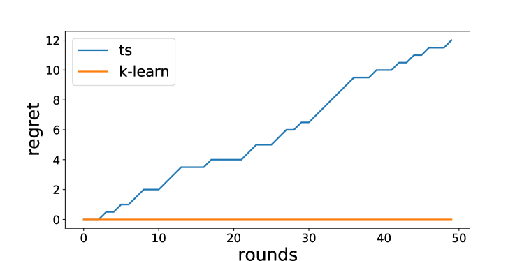
Figure 1: Regret for game matrix Eq. (9).

4 Adversarial bandit algorithms

In the adversarial bandit framework, an adversary and learner interact sequentially over $T$ rounds. In each round $t$, the learner chooses a distribution $x_{t}\in\Delta_{k}$ and the adversary simultaneously chooses a loss vector $\ell_{t}\in[0,1]^{k}$. Any algorithm designed for adversarial bandits can be used in our setting by choosing $\ell_{ti}=-A_{j_{t}i}$. The usual definition of the regret in this notation is

$$\underbrace{\mathbb{E}\left[\max_{i}\sum_{t=1}^{T}A_{j_{t}i}-\sum_{t=1}^{T}r_{t}\right]}_{\text{adversarial regret}}\geq\mathcal{R}(A,{\rm alg},T)\,.$$

Hence, an algorithm with small adversarial regret automatically enjoys small regret relative to the Nash strategy [Hannan, 1957]. There are now many algorithms for adversarial bandits, the most well-known being Exp3 [Auer et al., 1995]. The basic algorithm uses importance-weighting to estimate the rewards for each action and samples from a carefully tuned exponential weights distribution. Let $\hat{r}_{ti}$ be the importance-weighted estimate of the reward of action $i$ in round $t$:

$$\hat{r}_{ti}=\frac{r_{t}\mathbf{1}(i_{t}=i)}{x_{ti}}\,,$$

where the distribution of the player $x_{t}$ is given by

$$x_{ti}=\frac{\gamma_{t}}{k}+(1-\gamma_{t})\frac{\exp\left(\rho_{t}\sum_{s=1}^{t-1}\hat{r}_{si}\right)}{\sum_{j=1}^{k}\exp\left(\rho_{t}\sum_{s=1}^{t-1}\hat{r}_{sj}\right)}\,.$$

When $\rho_{t}$ and $\gamma_{t}$ are tuned appropriately, then the regret of Exp3 relative to the best action in hindsight is

$$\mathbb{E}\left[\max_{i}\sum_{t=1}^{T}A_{j_{t}i}-\sum_{t=1}^{T}r_{t}\right]=O\left(\sqrt{kT\log k}\right)\,.$$ (15)

The reader will notice that this bound is independent of the number of actions of the opponent, which was not true for UCB or K-learning. Another strength of Exp3 and similar algorithms is that the alternative notion of regret means they can exploit weak opponents. On the other hand, Exp3 is empirically much worse than K-learning and UCB. The reason is that Exp3 does not use the structure of the game and cannot quickly eliminate actions that do not play a strong role in any plausible Nash equilibrium. Furthermore, in many cases the goal is to learn the Nash equilibrium (if possible), i.e., to have ‘solved’ the game, not just to exploit the opponent. For example, since Exp3 does not converge to the minimax solution in general, it does not solve the robust bandit problem and suffers from high variance of $\Omega(T^{2})$ [Lattimore and Szepesvári, 2020, Ex. 11.6]. Concretely, consider playing rock-paper-scissors against an opponent with fixed strategy $(0.2,0.2,0.6)$. Exp3 against this opponent will converge towards playing $(1,0,0)$. However, a UCB or K-learning agent will learn to play the Nash strategy $(1/3,1/3,1/3)$, and will not be exploitable by any opponent (i.e., they will be robust), even though they only played against a weak player. If suddenly the opponent changes then Exp3 will suffer significantly larger losses than the robust algorithms even though the final regret may not be worse. We shall demonstrate this phenomenon in the numerical experiments.

There are many adaptations of Exp3. The main threads are (a) using the online convex optimisation view and modifying the regularizer [Audibert and Bubeck, 2009, Bubeck et al., 2018, Wei and Luo, 2018], for example, and (b) modifying the loss estimates to obtain high probability regret or adaptive bounds [Auer et al., 2002b, Kocák et al., 2014, Neu, 2015, Abernethy et al., 2008]. None of these algorithms are able to handle the additional knowledge of the opponent’s action and we do not believe any will improve on Exp3 by a significant margin empirically. The partial monitoring framework can incorporate knowledge of the opponent’s action [Rustichini, 1999]. Partial monitoring is now reasonably well understood theoretically [Bartók et al., 2014] and sensible algorithms exist [Lattimore and Szepesvári, 2019]. Regrettably, however, even with Bernoulli rewards, the matrix games studied here can only be modelled by exponentially large partial monitoring games for which existing algorithms are not practical. The case of two-player matrix games where the matrix $A$ is selected adversarially at each timestep was considered in [Cardoso et al., 2019], however, that work assumed control of both players, so is not applicable here.

5 Numerical experiments

In this section we present numerical results comparing the performance of the algorithms we have discussed so far. In most cases we are interested in measuring the empirical regret on a particular problem. Since this depends on the opponent we shall report cumulative absolute regret, i.e.,

$$\sum_{t=1}^{T}|V_{A}^{\star}-y_{t}^{T}Ax_{t}|,$$

for fixed $A$. This is meaningful because we primarily focus on two cases: self-play and against a best-response opponent. In self-play the algorithm is competing against another player using the same algorithm with the same information and so the cumulative absolute regret is a loosely measure of how far the players are from the Nash equilibrium. The best-response opponent knows the exact value of $A$ and the agent’s strategy at every round, and so can compute the action that minimizes the expected payoff. In this case the regret the agent suffers is always positive, so the absolute regret is the same as the usual notion of regret.

When running Exp3 we used the following parameters

$$\gamma_{t}=\min(\sqrt{k\log k/t},1),\quad\rho_{t}=\sqrt{2\log k/tk}.$$

5.1 Rock-paper-scissors

In the classic children’s game rock-paper-scissors, the payoff matrix is given by

	R	P	S
R	0	1	-1
P	-1	0	1
S	1	-1	0,

which defines a symmetric game with Nash equilibrium $(1/3,1/3,1/3)$ for both players. When comparing the techniques on this problem we add noise $\eta_{t}\sim\mathcal{N}(0,1)$ to the payoff, and use prior $\mathcal{N}(0,1)$ for each entry in the matrix for the Bayesian algorithms. We ran each experiment for $1000$ rounds and averaged the results over $100$ seeds.

In Figure 2 we present the self-play results and in Figure 3 we show the results against a best-response opponent. In both cases we plot the absolute regret of each algorithm and the KL-divergence of the policy produced by each algorithm to the Nash equilibrium policy. In self-play K-learning and UCB perform well with low regret and relatively quick convergence towards the Nash. Although Thompson sampling doesn’t enjoy a regret bound against all opponents, it still appears to perform well in self-play. Exp3, which does not use the matrix structure of the problem, does not converge to the Nash equilibrium in self-play in this case. This is shown by the linear absolute regret and the KL-divergence to the Nash saturating at a constant. Although Exp3 has a regret bound, the two competing instantiations oscillate around the Nash together, sometimes winning and sometimes losing (on average) against their opponent. It is clear from this result that Exp3 is not guaranteed to solve the game and converge to the Nash equilibrium, and so cannot solve the robust bandit problem in general without further assumptions. Against the best-response opponent the major difference is the dramatic decline in performance for Thompson sampling. It is clear that even in this simple case TS is easily exploited by an informed opponent and suffers significant losses. In contrast to self-play, against the best-response opponent Exp3 will converge to the Nash equilibrium, since it satisfies a regret bound and the Nash is the only strategy that is not exploitable. This is shown by the (slow) convergence in KL-divergence between the Exp3 policy and the Nash towards zero.

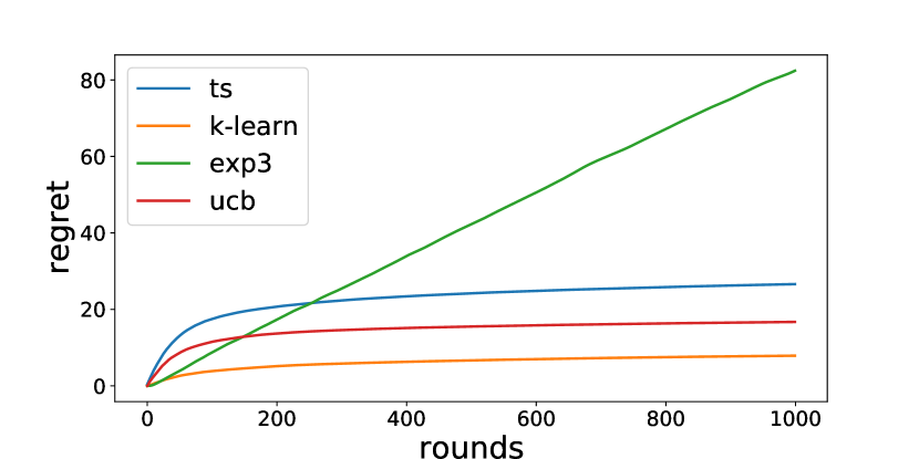
(a) Absolute regret.

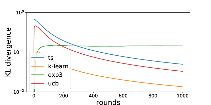
(b) KL divergence to Nash.

Figure 2: Rock-paper-scissors self-play.

In Figure 4 we compare the performance of the algorithms with regret bounds competing against each other with identical information. The legend displays ‘alg1 vs alg2’ for different choices of alg1 and alg2, and indicates that alg1 is playing as the maximizer and alg2 is the minimizer. We are plotting the regret (not absolute regret) from the point of view of the maximizer (alg1). If the regret is positive, it means that the minimizer (alg2) is winning on average. Since rock-paper-scissors is symmetric there is no advantage to being one player or the other so this is a fair head-to-head comparison. From the figure it is immediately obvious that the algorithms that leverage the matrix structure, K-learning and UCB, are easily beating Exp3 on average. Although Exp3 has a regret bound, it requires a long time to learn and in the meantime it suffers large losses against the optimistic approaches. When K-learning competes against UCB the algorithms are roughly evenly matched, however it appears that UCB has a slight advantage in this case.

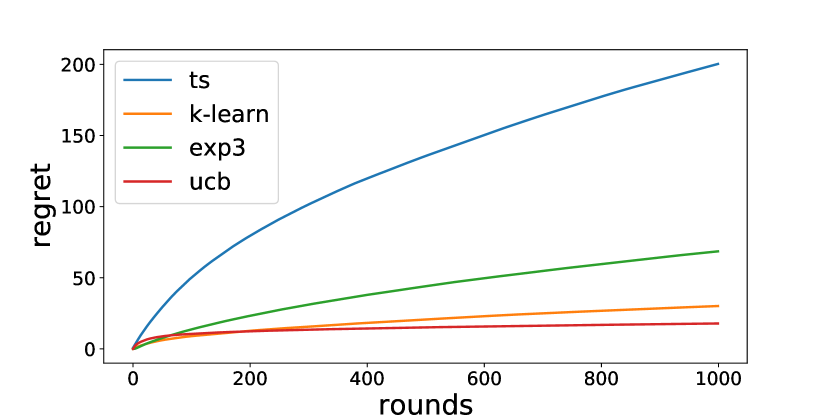
(a) Regret.

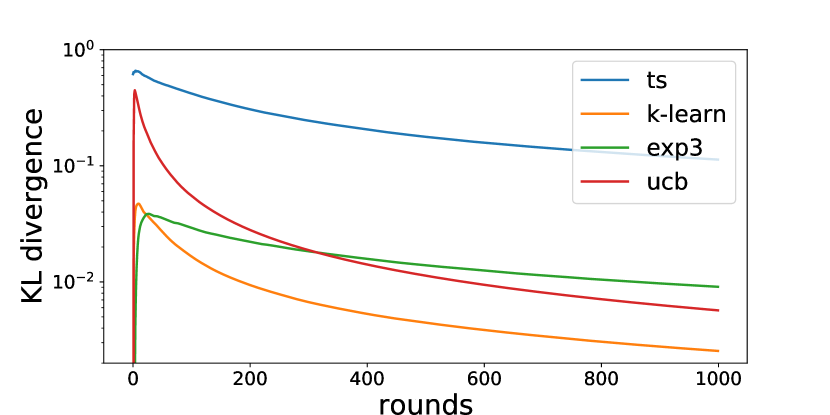
(b) KL divergence to Nash.

Figure 3: Rock-paper-scissors vs. best-response.

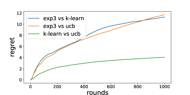
Figure 4: Rock-paper-scissors head-to-head regret.

5.2 Robust bandits

In the robust bandit problem the rewards the agent receives are partially determined by outcomes selected by nature, and the agent wants a policy that is robust to all possible outcomes. This problem can be formulated as a game to which we can apply the algorithms we have developed. To test their performance we generated a random game with $k=10$ agent actions and $m=5$ possible outcomes for each action, where each entry of $A$ was sampled IID from $\mathcal{N}(0.5,2.0)$. Nature sampled actions from a fixed policy that changed randomly every $50$ time-steps. We compare the algorithms presented in this manuscript against naive UCB and naive Thompson sampling, which treated the problem as though it was a standard stochastic multi-armed bandit problem. We ran each algorithm for $1000$ time-steps averaged over $100$ random seeds and we plot the histogram of the per time-period rewards in Figure 5. In Table 1 we show what proportion of the time each algorithm suffered a negative reward, as well as the average reward of each approach. It is clear that the naive approaches suffer from negative rewards more frequently, i.e., they are not robust to the changing conditions of nature. For example, K-learning suffers negative rewards almost $16\times$ less frequently than the naive approaches, which both suffered negative rewards about $15\%$ of the time, at the expense of slightly lower average reward. We can also see that Exp3 is not robust since it too suffers significantly more negative rewards than K-learning and UCB. Since Exp3 attempts to exploit the nature player, it can suffer large negative rewards for several periods when nature switches distribution. For completeness we include the results of the same problem against a best-response opponent, summarized in Table 2. Unsurprisingly the naive approaches are trivially exploitable by the BR opponent and suffer large negative rewards at every time-step. Again, Exp3 suffers significantly more negative reward than the robust approaches in this case. K-learning has both the largest average reward and the least percentage of negative rewards overall, followed by UCB.

Figure 5: Reward histograms on robust bandit problem.

	% returns $<0$	mean return
TS	2.3%	0.787
UCB	3.4%	0.995
K-learn	0.7%	0.935
Exp3	9.0%	1.092
Naive TS	15.9%	1.159
Naive UCB	14.1%	1.269

Table 1: Robust bandit problem vs Nature.

	% returns $<0$	mean return
TS	37.4%	0.027
UCB	18.8%	0.299
K-learn	5.1%	0.421
Exp3	19.5%	0.180
Naive TS	100.0%	-1.703
Naive UCB	100.0%	-1.710

Table 2: Robust bandit problem vs best-response.

6 Conclusion

The usual analysis of matrix games assumes that both players have perfect knowledge of the payoffs. We extended this to the case where the matrix that specifies the game is initially unknown to the players and must be learned about from experience, specifically from noisy bandit feedback. We showed that two previously published algorithms, UCB and K-learning, can be extended to this case and enjoy a sublinear regret bound, even against informed opponents that can compute a best-response to their strategies. We also showed a counter-example that rules out a sublinear regret bound for Thompson sampling under the same conditions. This difference between deterministically optimistic and stochastically optimistic algorithms is a significant departure from the single-player case. We supported our findings with numerical experiments that showed a significant advantage of these approaches when compared to both Thompson sampling and Exp3.

We conclude with a brief discussion about lower bounds. The two optimistic algorithms we developed in this manuscript have $O(\sqrt{T})$ regret upper bounds. One might speculate about the existence of matching lower bounds. Since the matrix game generalizes the stochastic multi-armed bandit problem we know we cannot improve upon this bound in the worst-case. However, this does not preclude the existence of an instance-dependent logarithmic regret bound. We conjecture that such a bound is not possible in general against all opponents, though it may be possible in more benign cases such as self-play with identical information. We leave exploring this to future work.

References

- Abernethy et al. [2008] J. D. Abernethy, E. Hazan, and A. Rakhlin. Competing in the dark: An efficient algorithm for bandit linear optimization. In Proceedings of the 21st Annual Conference on Learning Theory, pages 263–274. Omnipress, 2008.
- Audibert and Bubeck [2009] Jean-Yves Audibert and Sébastien Bubeck. Minimax policies for adversarial and stochastic bandits. In COLT, pages 217–226, 2009.
- Auer et al. [1995] Peter Auer, Nicolo Cesa-Bianchi, Yoav Freund, and Robert E Schapire. Gambling in a rigged casino: The adversarial multi-armed bandit problem. In Proceedings of IEEE 36th Annual Foundations of Computer Science, pages 322–331. IEEE, 1995.
- Auer et al. [2002a] Peter Auer, Nicolo Cesa-Bianchi, and Paul Fischer. Finite-time analysis of the multiarmed bandit problem. Machine learning, 47(2-3):235–256, 2002a.
- Auer et al. [2002b] Peter Auer, Nicolo Cesa-Bianchi, Yoav Freund, and Robert E Schapire. The nonstochastic multiarmed bandit problem. SIAM journal on computing, 32(1):48–77, 2002b.
- Bace [2000] Rebecca Gurley Bace. Intrusion detection. Sams Publishing, 2000.
- Badanidiyuru et al. [2013] Ashwinkumar Badanidiyuru, Robert Kleinberg, and Aleksandrs Slivkins. Bandits with knapsacks. In 2013 IEEE 54th Annual Symposium on Foundations of Computer Science, pages 207–216. IEEE, 2013.
- Bartók et al. [2014] G. Bartók, D. P. Foster, D. Pál, A. Rakhlin, and Cs. Szepesvári. Partial monitoring—classification, regret bounds, and algorithms. Mathematics of Operations Research, 39(4):967–997, 2014.
- Blum and Mansour [2007] Avrim Blum and Yishay Mansour. Learning, regret minimization, and equilibria. Algorithmic game theory, pages 79–102, 2007.
- Boyd and Vandenberghe [2004] Stephen Boyd and Lieven Vandenberghe. Convex optimization. Cambridge university press, 2004.
- Bubeck et al. [2018] S. Bubeck, M. Cohen, and Y. Li. Sparsity, variance and curvature in multi-armed bandits. In F. Janoos, M. Mohri, and K. Sridharan, editors, Proceedings of Algorithmic Learning Theory, volume 83 of Proceedings of Machine Learning Research, pages 111–127. PMLR, 07–09 Apr 2018.
- Bubeck and Cesa-Bianchi [2012] Sébastien Bubeck and Nicolo Cesa-Bianchi. Regret analysis of stochastic and nonstochastic multi-armed bandit problems. Foundations and Trends® in Machine Learning, 5(1):1–122, 2012.
- Cardoso et al. [2019] Adrian Rivera Cardoso, Jacob Abernethy, He Wang, and Huan Xu. Competing against Nash equilibria in adversarially changing zero-sum games. In Kamalika Chaudhuri and Ruslan Salakhutdinov, editors, Proceedings of the 36th International Conference on Machine Learning, volume 97 of Proceedings of Machine Learning Research, pages 921–930, Long Beach, California, USA, 09–15 Jun 2019. PMLR. URL http://proceedings.mlr.press/v97/cardoso19a.html.
- Caro and Gupta [2013] Felipe Caro and Aparupa Das Gupta. Robust control of the multi-armed bandit problem. Annals of Operations Research, pages 1–20, 2013.
- Cesa-Bianchi and Lugosi [2006] Nicolo Cesa-Bianchi and Gábor Lugosi. Prediction, learning, and games. Cambridge university press, 2006.
- Domahidi et al. [2013] A. Domahidi, E. Chu, and S. Boyd. ECOS: An SOCP solver for embedded systems. In European Control Conference (ECC), pages 3071–3076, 2013.
- Ghosh and Boyd [2003] Arpita Ghosh and Stephen Boyd. Minimax and convex-concave games, 2003. URL https://web.stanford.edu/class/ee392o/cvxccv.pdf.
- Hannan [1957] James Hannan. Approximation to bayes risk in repeated play. Contributions to the Theory of Games, 3:97–139, 1957.
- Immorlica et al. [2019] Nicole Immorlica, Karthik Abinav Sankararaman, Robert Schapire, and Aleksandrs Slivkins. Adversarial bandits with knapsacks. In 2019 IEEE 60th Annual Symposium on Foundations of Computer Science (FOCS), pages 202–219. IEEE, 2019.
- Kaufmann et al. [2012] Emilie Kaufmann, Olivier Cappé, and Aurélien Garivier. On Bayesian upper confidence bounds for bandit problems. In Artificial Intelligence and Statistics, pages 592–600, 2012.
- Kim and Lim [2016] Michael Jong Kim and Andrew EB Lim. Robust multiarmed bandit problems. Management Science, 62(1):264–285, 2016.
- Kocák et al. [2014] T. Kocák, G. Neu, M. Valko, and R. Munos. Efficient learning by implicit exploration in bandit problems with side observations. In Z. Ghahramani, M. Welling, C. Cortes, N. D. Lawrence, and K. Q. Weinberger, editors, Advances in Neural Information Processing Systems 27, pages 613–621. Curran Associates, Inc., 2014.
- Lai [1987] Tze Leung Lai. Adaptive treatment allocation and the multi-armed bandit problem. The Annals of Statistics, pages 1091–1114, 1987.
- Lattimore and Szepesvári [2019] T. Lattimore and Cs. Szepesvári. Exploration by optimisation in partial monitoring. 2019.
- Lattimore and Szepesvári [2020] Tor Lattimore and Csaba Szepesvári. Bandit algorithms. Cambridge University Press, 2020.
- Myerson [2013] Roger B Myerson. Game theory. Harvard university press, 2013.
- Nash et al. [1950] John F Nash et al. Equilibrium points in n-person games. Proceedings of the National Academy of Sciences of the United States of America, 36(1):48–49, 1950.
- Neu [2015] G. Neu. Explore no more: Improved high-probability regret bounds for non-stochastic bandits. In C. Cortes, N. D. Lawrence, D. D. Lee, M. Sugiyama, and R. Garnett, editors, Advances in Neural Information Processing Systems 28, NIPS, pages 3168–3176. Curran Associates, Inc., 2015.
- O’Donoghue et al. [2016] B. O’Donoghue, E. Chu, N. Parikh, and S. Boyd. Conic optimization via operator splitting and homogeneous self-dual embedding. Journal of Optimization Theory and Applications, 169(3):1042–1068, June 2016. URL http://stanford.edu/~boyd/papers/scs.html.
- O’Donoghue [2018] Brendan O’Donoghue. Variational Bayesian reinforcement learning with regret bounds. arXiv preprint arXiv:1807.09647, 2018.
- O’Donoghue et al. [2017a] Brendan O’Donoghue, Remi Munos, Koray Kavukcuoglu, and Volodymyr Mnih. Combining policy gradient and Q-learning. In International Conference on Learning Representations (ICLR), 2017a.
- O’Donoghue et al. [2017b] Brendan O’Donoghue, Ian Osband, Remi Munos, and Volodymyr Mnih. The uncertainty Bellman equation and exploration. arXiv preprint arXiv:1709.05380, 2017b.
- O’Donoghue et al. [2020] Brendan O’Donoghue, Ian Osband, and Catalin Ionescu. Making sense of reinforcement learning and probabilistic inference. In International Conference on Learning Representations (ICLR), 2020.
- Oliveira [2017] Thiago Bell Felix de Oliveira. Applying bandit algorithms to the route choice problem. 2017.
- Ordeshook [1986] Peter C Ordeshook. Game theory and political theory: An introduction. Cambridge University Press, 1986.
- Osband and Van Roy [2017] Ian Osband and Benjamin Van Roy. On optimistic versus randomized exploration in reinforcement learning, 2017.
- Rakhlin and Sridharan [2013] Sasha Rakhlin and Karthik Sridharan. Optimization, learning, and games with predictable sequences. In Advances in Neural Information Processing Systems, pages 3066–3074, 2013.
- Russo and Van Roy [2014] Daniel Russo and Benjamin Van Roy. Learning to optimize via posterior sampling. Mathematics of Operations Research, 39(4):1221–1243, 2014.
- Russo and Van Roy [2016] Daniel Russo and Benjamin Van Roy. An information-theoretic analysis of Thompson sampling. The Journal of Machine Learning Research, 17(1):2442–2471, 2016.
- Russo et al. [2018] Daniel J Russo, Benjamin Van Roy, Abbas Kazerouni, Ian Osband, Zheng Wen, et al. A tutorial on thompson sampling. Foundations and Trends® in Machine Learning, 11(1):1–96, 2018.
- Rustichini [1999] A. Rustichini. Minimizing regret: The general case. Games and Economic Behavior, 29(1):224–243, 1999.
- Serrano [2015] Santiago Akle Serrano. Algorithms for unsymmetric cone optimization and an implementation for problems with the exponential cone. PhD thesis, Stanford University, 2015.
- Thompson [1933] William R Thompson. On the likelihood that one unknown probability exceeds another in view of the evidence of two samples. Biometrika, 25(3/4):285–294, 1933.
- Villar et al. [2015] Sofía S Villar, Jack Bowden, and James Wason. Multi-armed bandit models for the optimal design of clinical trials: benefits and challenges. Statistical science: a review journal of the Institute of Mathematical Statistics, 30(2):199, 2015.
- Von Neumann [1928] John Von Neumann. Zur theorie der gesellschaftsspiele. Mathematische annalen, 100(1):295–320, 1928.
- Von Neumann and Morgenstern [1944] John Von Neumann and Oskar Morgenstern. Theory of games and economic behavior (commemorative edition). Princeton university press, 1944.
- Wei and Luo [2018] C-Y. Wei and H. Luo. More adaptive algorithms for adversarial bandits. In Sébastien Bubeck, Vianney Perchet, and Philippe Rigollet, editors, Proceedings of the 31st Conference On Learning Theory, volume 75 of Proceedings of Machine Learning Research, pages 1263–1291. PMLR, 06–09 Jul 2018.
- Wilbur and Zhu [2009] Kenneth C Wilbur and Yi Zhu. Click fraud. Marketing Science, 28(2):293–308, 2009.