Statistical field theory of ion-molecular solutions

Abstract

In this article, I summarize my theoretical developments in the statistical field theory of salt solutions of zwitterionic and multipolar molecules. Based on the Hubbard-Stratonovich integral transformation, I represent configuration integrals of dilute salt solutions of zwitterionic and multipolar molecules in the form of functional integrals over the space-dependent fluctuating electrostatic potential. In the mean-field approximation, for both cases, I derive integro-differential self-consistent field equations for the electrostatic potential, generated by the external charges in solutions media, which generalize the classical Poisson-Boltzmann equation. Using the obtained equations, in the linear approximation, I derive for the both cases a general expression for the electrostatic potential of a point-like test ion, expressed through certain screening functions. I derive an analytical expression for the electrostatic potential of the point-like test ion in a salt zwitterionic solution, generalizing the well known Debye-Hueckel potential. In the salt-free solution case, I obtain analytical expressions for the local dielectric permittivity around the point-like test ion and its effective solvation radius. For the case of salt solutions of multipolar molecules, I find a new oscillating behavior of the electrostatic field potential of the point-like test ion at long distances, which is caused by the nonzero quadrupole moments of the multipolar molecules. I obtain a general expression for the average quadrupolar length of a multipolar solute. Using the random phase approximation (RPA), I derive general expressions for the excess free energy of bulk salt solutions of zwitterionic and multipolar molecules and analyze the limiting regimes resulting from them. I generalize the salt zwitterionic solution theory for the case when several kinds of zwitterions are dissolved in the solution. In this case, within the RPA, I obtain a general expression for the solvation energy of the test zwitterion. Finally, I demonstrate how to take a systematic account of the excluded volume correlations between multipolar molecules in addition to their electrostatic correlations. I believe that the formulated findings could be useful for the future theoretical models of the real ion-molecular solutions, such as salt solutions of micellar aggregates, metal-organic complexes, proteins, betaines, etc.

I Introduction

Coarse-grained modeling (CGM) methods have been so far widely used for molecular dynamics (MD) simulations of equilibrium properties of ion-molecular systems, such as ionic and zwitterionic liquids, dielectric polymers, micellar aggregates, proteins, and complex colloids (see, for example, Wang et al. (2007); Bhargava et al. (2007); Shinoda, De Vane, and Klein (2010); Chakrabarty and Cagin (2010); Baaden and Marrink (2013); Nielsen et al. (2004); Wu and Shea (2011); Schröder and Steinhauser (2010); Cavalcante, Ribeiro, and Skaf (2014)). CGM is based on the idea that separate atomic (molecular) groups are combined into large particles, whose interactions are described by effective pairwise potentials. Despite a certain success in reducing the computing time of the MD simulation by coarsening of the real structure of the molecules in comparison with their full-atomic representation, modeling of the systems contaning a large number of particles (even with a coarsened structure) under the conditions of a condensed phase is still rather computationally expensive. The structural properties of ion-molecular systems (for instance, site-site pair correlation functions and hydration numbers) are commonly described by the statistical theory of integral equations for the site-site correlation functions (Reference Interactions Site Model or RISM) with different closing relations (see, for instance, Fedotova and Dmitrieva (2015, 2016); Eiberweiser et al. (2015); Fedotova, Kruchinin, and Chuev (2019); Fedotova and Kruchinin (2014, 2012)). Although the RISM theory allows quite accurate estimation of the structural quantities, it is impossible within the RISM theory to obtain analytical expressions for the thermodynamic properties, such as the excess chemical potentials of species, osmotic coefficient, equation of state, etc. Ratkova, Palmer, and Fedorov (2015); Kovalenko (2004); Chuev et al. (2006); Kovalenko and Hirata (2005). Moreover, the numerical solution of the 3D-RISM integral equations is rather computationally expensive and no less time-consuming than the MD simulations.

Thus, it can be concluded that modern theoretical chemical physics and physical chemistry need some computational tools based on the fundamentals of statistical physics and allowing one to predict the qualitative behavior of the thermodynamic parameters in a fast and effective way. The field-theoretic (FT) methods based on the Hubbard-Stratonovich (HS) integral transformation of the configuration integral and correlation functions of a certain model fluid in the form of a functional integral over one or few space-dependent fluctuating fields could become such a tool. At present, these methods are well-proven as the ones for describing the thermodynamic and structural properties of simple neutral and ionic fluids Storer (1969); Frusawa (2018); Ivanchenko and Lisyansky (1984); Hubbard and Schofield (1972); Caillol, Patsahan, and Mryglod (2006, 2005); Caillol (2003); Edwards (1959); Efimov and Nogovitsin (1996); Zakharov and Loktionov (1999); Brilliantov (1998a); Trokhymchuk et al. (2017); Brilliantov, Rubi, and Budkov (2020) and polymer solutions Edwards (1966); Fredrickson (2006). Among them are the mean-field (saddle-point) approximation Brilliantov (1998a); Abrashkin, Andelman, and Orland (2007); Budkov, Kolesnikov, and Kiselev (2015); Brilliantov, Rubi, and Budkov (2020), random-phase approximation Edwards (1966); Budkov (2018, 2019a), many-loop expansion Netz (2001), variation method Lue (2006), and the renormalization group theory Brilliantov, Bagnuls, and Bervillier (1998). However, to apply the FT approaches to the theoretical description of ion-molecular systems at the equilibrium in the bulk and at the interfaces, one needs to take into account not only the universal dispersion and excluded volume inter-molecular interactions, but also the special features of the species molecular structure, such as multipole moments, electronic and molecular polarizabilities, configuration asymmetry of the molecule, etc. However, scientists have only made the first steps in that direction. Up to now, they have formulated FT models of polarizable polymer solutions Martin et al. (2016); Kumar and Fredrickson (2009); Budkov, Kalikin, and Kolesnikov (2017); Budkov and Kiselev (2017); Gordievskaya, Budkov, and Kramarenko (2018); Kumar, Sumpter, and Muthukumar (2014); Grzetic, Delaney, and Fredrickson (2018); Gurovich (1994), salt solutions of polar and multipolar molecules Budkov (2018, 2019a, 2019b, 2019c), electrolyte solutions with an explicit account of the polar solvent and ion polarizability Buyukdagli and Ala-Nissila (2013a); Buyukdagli and Blossey (2014); Buyukdagli and Ala-Nissila (2013b); Abrashkin, Andelman, and Orland (2007); Coalson and Duncan (1996); Budkov, Kolesnikov, and Kiselev (2015); Grzetic, Delaney, and Fredrickson (2019), solutions of liquid crystalline ionic fluids Lue (2006); Kopanichuk et al. (2016), aqueous solutions of the intrinsically disordered proteins Lin et al. (2017); McCarty et al. (2019), and a cluster model of ionic liquids Avni, Adar, and Andelman (2020). Despite the evident success achieved in applications of the FT methods to complex ion-molecular systems, they still remain underestimated by chemical engineers and materials scientists, in comparison with the coarse-grained MD simulation methods or the above mentioned RISM theory. In my opinion, this is because of their mathematical complexity, on the one hand, and the lack of accessible software for general public users, on the other hand.

Recent advances in experimental studies of the organic zwitterionic compounds (see, for instance, Canchi and Garcia (2013); Heldebrant, Koech, and M Trisha C (2010); Felder et al. (2007)) consisting simultaneously of positively and negatively charged ionic groups, located at rather long distances (several nanometers) offer a challenge to statistical thermodynamics to develop analytical approaches for describing thermodynamic properties of such systems. As a rule, the fundamental difference of zwitterions from classical small polar molecules, such as water and alcohols, is that it is impossible to model them as particles carrying point-like dipoles Onsager (1936); Kirkwood (1939); Høye and Stell (1976). Instead, they must be considered as pairs of bonded oppositely charged ionic groups located at fixed or fluctuating distances from each other, thus supplementing the theory with an additional length scale. The latter is attributed to the effective distance between the charged groups. Moreover, since in practice such molecules are dissolved in a low-molecular weight polar solvent (primarily in water) in the presence of salt ions, it is necessary to develop a model of electrolyte solutions with a small additive of polar particles described as ionic pairs with fluctuating distances between the charged groups. Such a $"$nonlocal$"$ theory could solve a number of fundamental problems of the polar fluids theory. Firstly, such theory will allow one to describe the behavior of the point-like charge potential in an electrolyte solution medium with an addition of polar particles at the scale of their effective size. Secondly, this theory must be devoid of the nonphysical unavoidable divergence of the electrostatic free energy of the polar fluid with point-like polar molecules, which is the case in the existing $"$local$"$ theories (see, for instance, Dean and Podgornik (2012); Levy, Andelman, and Orland (2012); Budkov and Kolesnikov (2016); Budkov, Kalikin, and Kolesnikov (2017)). A generalization of the dipolar particles model, which could be relevant to the modern physical chemistry of solutions, is the model of $"$hairy$"$ particles Budkov (2019a). Each hairy particle is comprised of a big charge, located at the center of the particle (central charge), and peripheral charges, located at fixed or fluctuating distances around it. Such configurations could be realized for spherical polyelectrolyte stars and brushes (see, for instanse, Ballauff (2007); Jusufi, Likos, and Löwen (2002)), spherical colloidal particles with counterions condensed onto their charged surfaces Linse and Lobaskin (1999); Linse (2005), metal-organic complexes with multivalent metal ions, surrounded by oppositely charged monovalent ionic ligands Xu et al. (2014); Perez and Riera (2008), etc.

To the best of my knowledge, until recently, there were no attempts to formulate statistical models of the salt solutions of dipolar and multipolar molecules making it possible to obtain the analytical relations for their thermodynamic quantities from the first principles of statistical mechanics. In this regard, in the present extended article, in the context of modern statistical field theory of ion-molecular solutions, I would like to summarize my recent theoretical findings in the development of the FT models of ion-molecular solutions, whose solute molecules possess a multipolar internal electric structure.

II Statistical field theory of salt zwitterionic solutions

The existing statistical theories of polar fluids describe molecules as point-like dipoles Abrashkin, Andelman, and Orland (2007) or hard spheres with a point-like dipole in their center Høye and Stell (1976). As is well known, disregard of the details of the internal electrical structure of polar molecules in calculations of the electrostatic free energy of the polar fluid from the first principles of statistical mechanics leads to $"$ultraviolet divergence$"$ of electrostatic free energy, which makes the researchers resort to the artificial $"$ultraviolet cut-off$"$, while integrating over the vectors of the reciprocal space Levy, Andelman, and Orland (2012); Budkov, Kalikin, and Kolesnikov (2017). On the other hand, as it has been mentioned above, a $"$local$"$ theory that does not consider the charge distribution of the polar molecule, cannot describe the behavior of the point-like charge potential surrounded by polar molecules at the distances of their linear size order. Thus, one can expect that a $"$non-local$"$ statistical theory taking such details into account will be free from the ultraviolet divergence of the free energy present in the local theories and will allow one to investigate the electrostatic potential of the point-like ion at the distances from the ion comparable with the characteristic distances between the charged centers of polar molecules.

Let us consider an electrolyte solution comprised of a mixture of point-like ions of $s$ kinds with the total numbers $N_{i}$ ($i=1,...,s$) and charges $z_{i}e$ ($z_{i}$ is the ion valency and $e$ is the elementary charge) and $N$ zwitterions with point-like ionic groups with charges $\pm q$, confined in the volume $V$ at the temperature $T$. Let the number of ions $N_{i}$ satisfy the electrical neutrality condition $\sum_{i}z_{i}N_{i}=0$. Moreover, let us assume that all the particles are immersed in a solvent, which is modelled as a continuous dielectric medium with the constant permittivity $\varepsilon$. This means the adoption of the simplest implicit solvent model which does not take into account the molecular structure effects. It can be justified by the assumption that the effective size of a solvent molecule is much smaller than the zwitterion effective size. The models of polar solvents taking into account the molecular structure were formulated in papers Kornyshev and Sutmann (1996); Leikin and Kornyshev (1990); Kornyshev et al. (1989); Kornyshev (1986); Buyukdagli and Blossey (2014); Buyukdagli and Ala-Nissila (2013b, a). I suppose that there is a probability distribution function $\omega(\mathbb{r})$ of the distance between the charged centres, associated with each zwitterion. I would also like to note that the contribution of the repulsive forces between all the particles attributed to their excluded volume is neglected. It can be justified by rather small concentrations of ions and polar particles. At the end of this section, I will show how it is possible to extend the formulated statistical field theory to account for the excluded volume interactions.

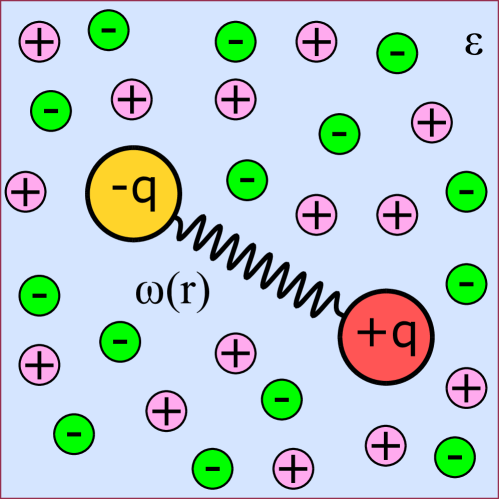
Figure 1: Schematic representation of the zwitterion surrounded by salt ions in a dielectric solvent medium.

General field-theoretic formalism. In view of above-mentioned model assumptions, the configuration integral of the mixture can be written in the following form:

$$Q=\int d\Gamma_{zw}\int d\Gamma_{s}\exp\left[-\beta H_{int}\right],$$ (1)

where

$$\int d\Gamma_{zw}(\cdot)=\int...\int\prod\limits_{j=1}^{N}\frac{d\mathbb{r}_{j}^{(+)}d\mathbb{r}_{j}^{(-)}}{V}\omega\left(\mathbb{r}_{j}^{(+)}-\mathbb{r}_{j}^{(-)}\right)(\cdot)$$ (2)

is the measure of integration over the coordinates $\mathbb{r}_{j}^{(\pm)}$ of the ionic groups with the above-mentioned probability distribution function $\omega(\mathbb{r})$, which, according to its definition, must satisfy the normalization condition:

$$\int\omega(\mathbb{r})d\mathbb{r}=1,$$ (3)

and

$$\int d\Gamma_{s}(\cdot)=\int...\int\prod\limits_{j=1}^{s}\prod\limits_{k_{j}=1}^{N_{j}}\frac{d\mathbb{r}_{k_{j}}}{V}(\cdot)$$ (4)

is the integration measure over the coordinates of the salt ions; $\beta=(k_{B}T)^{-1}$, $k_{B}$ being the Boltzmann constant. The total potential energy of the interactions taking into account the self-interactions of the charges is

$$H_{int}=\frac{1}{2}\int d\mathbb{r}\int d\mathbb{r}^{\prime}\hat{\rho}(\mathbb{r})G_{0}(\mathbb{r}-\mathbb{r}^{\prime})\hat{\rho}(\mathbb{r}^{\prime})=\frac{1}{2}\left(\hat{\rho}G_{0}\hat{\rho}\right),$$ (5)

where $G_{0}(\mathbb{r}-\mathbb{r^{\prime}})=1/(\varepsilon|\mathbb{r}-\mathbb{r}^{\prime}|)$ is the Green function of the Poisson equation and

$$\hat{\rho}(\mathbb{r})=\hat{\rho}_{zw}(\mathbb{r})+\hat{\rho}_{i}(\mathbb{r})+\rho_{ext}(\mathbb{r}),$$ (6)

is the total charge density of the system with the microscopic charge densities of the zwitterions

$$\hat{\rho}_{zw}(\mathbb{r})=q\sum_{j=1}^{N}\left(\delta\left(\mathbb{r}-\mathbb{r}_{j}^{(+)}\right)-\delta\left(\mathbb{r}-\mathbb{r}_{j}^{(-)}\right)\right),$$ (7)

and the ionic species

$$\hat{\rho}_{i}(\mathbb{r})=e\sum\limits_{j=1}^{s}z_{j}\sum\limits_{k_{j}=1}^{N_{j}}\delta\left(\mathbb{r}-\mathbb{r}_{k_{j}}\right),$$ (8)

and $\rho_{ext}(\mathbb{r})$ is the charge density of the external charges (of electrodes or membranes, for instance); $e$ is the elementary charge.

Using the standard HS transformation Stratonovich (1957); Hubbard (1959); Efimov and Nogovitsin (1996)

$$\exp\left[-\frac{\beta}{2}(\hat{\rho}G_{0}\hat{\rho})\right]=\int\frac{\mathcal{D}\varphi}{C}\exp\left[-\frac{\beta}{2}(\varphi G_{0}^{-1}\varphi)+i\beta(\hat{\rho}\varphi)\right],$$ (9)

one can get the following representation of the configuration integral in the thermodynamic limit $V\to\infty,\leavevmode\nobreak\ N_{i}\to\infty,\leavevmode\nobreak\ N_{i}/V\to c_{i},\leavevmode\nobreak\ N/V\to n$ in the form of a functional integral over the fluctuating electrostatic potential $\varphi(\mathbb{r})$ Budkov (2018):

$$Q=\int\frac{\mathcal{D}\varphi}{C}\exp\left[-S[\varphi]\right],$$ (10)

where the following auxiliary functional is introduced:

$$S[\varphi]=\frac{\beta}{2}(\varphi G_{0}^{-1}\varphi)-i\beta(\rho_{ext}\varphi)-n\int d\mathbb{r}\int d\mathbb{r}^{\prime}\omega(\mathbb{r}-\mathbb{r}^{\prime})\left(e^{i\beta q(\varphi(\mathbb{r})-\varphi(\mathbb{r}^{\prime}))}-1\right)$$

$$-\sum\limits_{j=1}^{s}c_{j}\int d\mathbb{r}\left(e^{i\beta z_{j}e\varphi(\mathbb{r})}-1\right)$$ (11)

with the following shorthand notations

$$(fAf)=\int d\mathbb{r}\int d\mathbb{r}^{\prime}f(\mathbb{r})A(\mathbb{r},\mathbb{r}^{\prime})f(\mathbb{r}^{\prime}),\leavevmode\nobreak\ (fg)=\int d\mathbb{r}f(\mathbb{r})g(\mathbb{r}).$$ (12)

The normalization constant $C=\int\mathcal{D}\varphi\exp\left[-\frac{\beta}{2}(\varphi G_{0}^{-1}\varphi)\right]$ is also introduced. The inverse Green function $G^{-1}_{0}(\mathbb{r},\mathbb{r}^{\prime})$ is determined by the following integral relation

$$\int d\mathbb{r}^{\prime\prime}G_{0}^{-1}(\mathbb{r},\mathbb{r}^{\prime\prime})G_{0}(\mathbb{r}^{\prime\prime}-\mathbb{r}^{\prime})=\delta(\mathbb{r}-\mathbb{r}^{\prime})$$ (13)

that yields

$$G_{0}^{-1}(\mathbb{r},\mathbb{r}^{\prime})=-\frac{\varepsilon}{4\pi}\nabla^{2}\delta\left(\mathbb{r}-\mathbb{r}^{\prime}\right),$$ (14)

where $\nabla^{2}=\Delta$ is the Laplace operator. It can be shown Budkov (2018) that the obtained functional $S[\varphi]$ in the case of polar particles with a fixed distance between the charged centers, at its sufficiently small value, transforms into the well-known Poisson-Boltzmann-Langevin (PBL) functional Abrashkin, Andelman, and Orland (2007); Coalson and Duncan (1996); Buyukdagli and Blossey (2014); Budkov, Kolesnikov, and Kiselev (2015)

$$S_{PBL}[\varphi]=\frac{\beta}{2}(\varphi G_{0}^{-1}\varphi)-n\int d\mathbb{r}\left(\frac{\sin\beta p|\mathbb{\nabla}\varphi(\mathbb{r})|}{\beta p|\mathbb{\nabla}\varphi(\mathbb{r})|}-1\right)-i\beta(\rho_{ext}\varphi)-\int d\mathbb{r}\sum\limits_{j=1}^{s}c_{j}\left(e^{i\beta z_{j}e\varphi(\mathbb{r})}-1\right),$$ (15)

where $p=ql$ is the dipole moment of the polar molecules.

Mean-field approximation. In the mean field approximation Naji et al. (2013) the self-consistent field equation $\delta{S[\varphi_{MF}]}/\delta{\varphi(\mathbb{r})}=0$ for the electrostatic potential $\psi(\mathbb{r})=-i\varphi^{MF}(\mathbb{r})$ takes the following form

$$-\frac{\varepsilon}{4\pi}\Delta\psi(\mathbb{r})=2nq\int d\mathbb{r}^{\prime}\omega(\mathbb{r}-\mathbb{r}^{\prime})\sinh\frac{q(\psi(\mathbb{r})-\psi(\mathbb{r}^{\prime}))}{k_{B}T}+\sum\limits_{j=1}^{s}z_{j}ec_{j}e^{-\beta z_{j}e\psi(\mathbb{r})}+\rho_{ext}(\mathbb{r}).$$ (16)

As is seen, equation (16) is a generalization of the classical Poisson-Boltzmann equation Naji et al. (2013); Levin (2002) for the self-consistent field potential for the case when the solution contains zwitterions. The electrostatic free energy in the mean-field approximation is

$$F_{el}^{(MF)}=k_{B}TS[i\psi].$$ (17)

Then, solving self-consistent field equation (16) within the approximation of the weak electrostatic interactions, i.e. when $q\psi(\mathbb{r})/{k_{B}T}\ll 1$, by the Fourier-transformation method, we arrive at the expression for the electrostatic potential of the test point-like ion with the charge density $\rho_{ext}(\mathbb{r})=q_{0}\delta(\mathbb{r})$ as follows

$$\psi(\mathbb{r})=\frac{4\pi q_{0}}{\varepsilon}\int\frac{d\mathbb{k}}{(2\pi)^{3}}\frac{e^{i\mathbb{k}\mathbb{r}}}{k^{2}+\varkappa^{2}(\mathbb{k})},$$ (18)

where

$$\varkappa^{2}(\mathbb{k})=\kappa_{s}^{2}+\frac{8\pi nq^{2}}{\varepsilon k_{B}T}\left(1-\omega(\mathbb{k})\right)$$ (19)

is the screening function Brilliantov (1993); Khokhlov and Khachaturian (1982); Borue and Erukhimovich (1988); Budkov (2018, 2019a, 2019b) and

$$\omega(\mathbb{k})=\int d\mathbb{r}e^{-i\mathbb{k}\mathbb{r}}\omega(\mathbb{r})$$ (20)

is the characteristic function Gnedenko (2018) corresponding to the distribution function $\omega(\mathbb{r})$; $\kappa_{s}=(8\pi e^{2}I/\varepsilon k_{B}T)^{1/2}$ is the inverse Debye length, attributed to the ionic species with the ionic strength $I=\sum_{j}z_{j}^{2}c_{j}/2$. For the model characteristic function

$$\omega(\mathbb{k})=\frac{1}{1+\frac{k^{2}l^{2}}{6}},$$ (21)

determining the following distribution function

$$\omega(\mathbb{r})=\frac{3}{2\pi l^{2}r}\exp\left(-\frac{\sqrt{6}r}{l}\right),$$ (22)

where $r=|\mathbb{r}|$, the following expression for the electrostatic potential can be obtained Budkov (2018)

$$\psi(\mathbb{r})=\frac{q_{0}}{\varepsilon r}\left(u(y_{d},y_{s})e^{-\kappa_{1}(y_{d},y_{s})r}+\left(1-u(y_{d},y_{s})\right)e^{-\kappa_{2}(y_{d},y_{s})r}\right),$$ (23)

where I have introduced the following notations

$$\kappa_{1,2}(y_{d},y_{s})=\frac{\sqrt{3}}{l}\left(1+y_{s}+y_{d}\pm\sqrt{(1+y_{s}+y_{d})^{2}-4y_{s}}\right)^{1/2},$$ (24)

$$u(y_{d},y_{s})=\frac{y_{s}+y_{d}+\sqrt{(1+y_{s}+y_{d})^{2}-4y_{s}}-1}{2\sqrt{(1+y_{s}+y_{d})^{2}-4y_{s}}},$$ (25)

and $y_{s}={\kappa_{s}^{2}l^{2}}/{6}$, $y_{d}={4\pi nq^{2}l^{2}}/{(3\varepsilon k_{B}T)}={l^{2}}/{6r_{D}^{2}}$; $r_{D}=\left(8\pi nq^{2}/\varepsilon k_{B}T\right)^{-1/2}$ is the Debye length associated with the charged centers of the zwitterions. Note that the potential (23) monotonically decreases at long distances at all values of $y_{s}$ and $y_{d}$. It is interesting to analyze the limiting regimes, following from eq. (23). For the salt-free solution ($y_{s}=0$) we get:

$$\psi(\mathbb{r})=\frac{q_{0}}{\varepsilon_{l}(r)r}$$ (26)

with the local dielectric permittivity being

$$\varepsilon_{l}(r)=\frac{\varepsilon(1+y_{d})}{1+y_{d}\exp\left(-\frac{r}{l_{s}}\right)}$$ (27)

and $l_{s}=l/\sqrt{6(1+y_{d})}$ is the new length scale which determines the radius of the sphere with the point-like test ion in its center, within which the dielectric permittivity is smaller than its bulk value, determined by the relation

$$\varepsilon_{b}=\varepsilon(1+y_{d})=\varepsilon+\frac{4\pi q^{2}l^{2}}{3k_{B}T}n.$$ (28)

Eq. (28) for the bulk dielectric permittivity is the same as the one obtained in paper Ramshaw (1980) by means of the integral equations theory within the mean spherical approximation for the rigid dipoles. Thus, the length $l_{s}$ can be interpreted as the effective solvation radius of the point-like charge surrounded by zwitterions, within the linear approximation. Note that at $y_{d}\gg 1$ eq. (26) transforms into the standard Debye-Hueckel (DH) potential

$$\psi(\mathbb{r})=\frac{q_{0}}{\varepsilon r}\exp\left[-{r}/{r_{D}}\right].$$ (29)

Thus, when the dipole length $l$ is much bigger than the Debye length $r_{D}$, the charged centers of zwitterions manifest themselves as unbound ions, participating in the screening of the test point-like charge $q_{0}$.

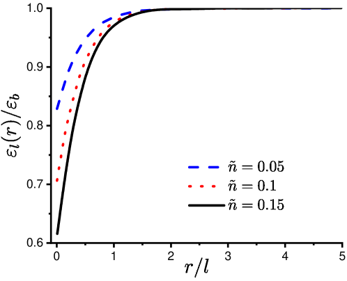
Figure 2: Local dielectric permittivity around the point-like test ion as a function of distance, expressed in dipole length $l$ units, for different reduced concentrations of zwitterions $\tilde{n}=nl^{3}$.

In the absence of the zwitterions ($y_{d}=0$) we obtain the standard Debye-Hueckel potential Landau and Lifshitz (2013):

$$\psi(\mathbb{r})=\frac{q_{0}}{\varepsilon r}e^{-\kappa_{s}r}.$$ (30)

Then, after simple algebraic transformations, one can show Budkov (2018) that the mean-field electrostatic free energy within the linear approximation is:

$$F_{el}^{(MF)}=\frac{1}{2}\int d\mathbb{r}\rho_{ext}(\mathbb{r})\psi(\mathbb{r}).$$ (31)

To obtain an expression for the solvation energy of the test ion, one must subtract its self-energy from the electrostatic free energy, i.e.

$$\Delta F_{el}=\mu_{el}^{(ion)}=\frac{1}{2}\int d\mathbb{r}\rho_{ext}(\mathbb{r})\left(\psi(\mathbb{r})-\psi_{ext}(\mathbb{r})\right)$$

$$=-\frac{q_{0}^{2}}{2\varepsilon}\left(u(y_{d},y_{s})(\kappa_{1}(y_{d},y_{s})-\kappa_{2}(y_{d},y_{s}))+\kappa_{2}(y_{d},y_{s})\right).$$ (32)

I would like to note that the solvation energy of the point-like charge is equal to its excess chemical potential (see below). In the absence of the salt ions ($y_{s}=0$), the expression for the solvation energy (32) of the test charge $q_{0}$ takes the form Budkov (2018)

$$\mu_{el}^{(ion)}=-\frac{q_{0}^{2}}{2\varepsilon R_{ef}},$$ (33)

where

$$R_{ef}=\frac{l}{\sqrt{6}}\frac{\sqrt{1+y_{d}}}{y_{d}}$$ (34)

is the effective radius of the point-like charge in the environment of the polar molecules. It is interesting to note that in contrast to the local theory with point-like dipoles, within this nonlocal theory, the electrostatic free energy of the point-like test ion has a finite value. Note that at $y_{d}\ll 1$ (or at $l\to 0$) the solvation energy (33) tends to zero linearly with $l$, i.e.

$$\mu_{el}^{(ion)}\simeq-\frac{2\pi\sqrt{6}}{3}\frac{q^{2}q_{0}^{2}n}{\varepsilon^{2}k_{B}T}l.$$ (35)

In the opposite case, $y_{d}\gg 1$, when the charged sites of zwitterions behave as unbound ions the solvation energy results in

$$\mu_{el}^{(ion)}\simeq-\frac{q_{0}^{2}}{2\varepsilon r_{D}},$$ (36)

which is the well known expression for excess chemical potential of ion in dilute electrolyte solution within the DH theory Landau and Lifshitz (2013). I would like to note that eq. (33) describes the solvation energy when we can neglect the linear size of solvated ion, i.e. when $l\gg a$, where $a$ is the ionic radius. Indeed, within the present theory, the point-like dipole limit ($l\to 0$) with keeping $ql$ constant gives infinite solvation energy of point-like test ion. Such a divergence of solvation energy is related to the fact that I do not take into account excluded volume of test ion. Accounting for the excluded volume of solvated ion will allow us to obtain a finite value of solvation energy even in point-like dipole limit Levin (2002, 1999); Adar et al. (2018).

Random phase approximation. The simplest method to estimate the electrostatic free energy of salt zwitterionic solution is the random phase approximation (RPA) Naji et al. (2013); Budkov (2018). Expanding the functional $S[\varphi]$ in eq. (10) into a power functional series in the neighbourhood of the mean-field configuration $\varphi_{MF}(\mathbb{r})=i\psi(\mathbb{r})$ and truncating it by the quadratic term on the functional variable $\Lambda(\mathbb{r})=\varphi(\mathbb{r})-i\psi(\mathbb{r})$, I obtain:

$$Q\approx\exp\left[-S[i\psi]\right]\int\frac{\mathcal{D}\Lambda}{C}\exp\left[-\frac{\beta}{2}\left(\Lambda\mathcal{G}^{-1}\Lambda\right)\right],$$ (37)

where

$$\mathcal{G}^{-1}(\mathbb{r},\mathbb{r}^{\prime}|\psi)=k_{B}T\frac{\delta^{2}S[i\psi]}{\delta\varphi(\mathbb{r})\delta\varphi(\mathbb{r}^{\prime})}=G_{0}^{-1}(\mathbb{r},\mathbb{r}^{\prime})+\beta e^{2}\sum\limits_{j=1}^{s}z_{j}^{2}e^{-\beta z_{j}e\psi(\mathbb{r})}\delta(\mathbb{r}-\mathbb{r}^{\prime})$$

$$+\frac{2nq^{2}}{k_{B}T}\int d\mathbb{r}^{\prime\prime}\omega(\mathbb{r}-\mathbb{r}^{\prime\prime})\cosh\left(\frac{q\left(\psi(\mathbb{r})-\psi(\mathbb{r}^{\prime\prime})\right)}{k_{B}T}\right)(\delta(\mathbb{r}-\mathbb{r}^{\prime})-\delta(\mathbb{r}^{\prime\prime}-\mathbb{r}^{\prime}))$$ (38)

is the renormalized inverse Green function depending on the mean-field electrostatic potential $\psi(\mathbb{r})$, satisfying eq. (16). Thus, when the Gaussian functional integral is evaluated by the standard methods Zinn-Justin (1996), the following general relation for the configuration integral within the RPA can be obtained:

$$Q\approx\exp\left[-S[i\psi]+\frac{1}{2}tr\left(\ln\mathcal{G}-\ln G_{0}\right)\right],$$ (39)

where the symbol $tr(...)$ means the trace of the integral operator Budkov (2019b, a), i.e. $tr(A)=\int d\mathbb{r}A(\mathbb{r},\mathbb{r})$, where $A(\mathbb{r},\mathbb{r}^{\prime})$ is the kernel of integral operator $A$. In the absence of the external charges (i.e., at $\rho_{ext}(\mathbb{r})=0$), the electrostatic potential $\psi(\mathbb{r})=0$, and the mean-field contribution to the electrostatic free energy $F_{el}^{(MF)}=k_{B}TS[0]=0$. Thus, in this case, the electrostatic free energy is determined by the thermal fluctuations of the electrostatic potential near its zero value and takes the following form (see Appendix I):

$$F_{el}=\frac{Vk_{B}T}{2}\int\frac{d\mathbb{k}}{(2\pi)^{3}}\left(\ln\left(1+\frac{\varkappa^{2}(\mathbb{k})}{k^{2}}\right)-\frac{\varkappa^{2}(\mathbb{k})}{k^{2}}\right),$$ (40)

where the screening function $\varkappa^{2}(\mathbb{k})$ is determined by eq. (19). The excess osmotic pressure caused by the electrostatic interactions which can be obtained from the standard thermodynamic relation Landau and Lifshitz (2013) $\Pi_{el}=-\left(\partial{F_{el}}/\partial{V}\right)_{T}$, takes the form

$$\Pi_{el}=\frac{k_{B}T}{2}\int\frac{d\mathbb{k}}{(2\pi)^{3}}\left(\frac{\varkappa^{2}(\mathbb{k})}{k^{2}+\varkappa^{2}(\mathbb{k})}-\ln\left(1+\frac{\varkappa^{2}(\mathbb{k})}{k^{2}}\right)\right).$$ (41)

For the distribution function, defined by eq. (21), in the absence of the ions in the solution ($I=0$), the integral in eq. (40) can be calculated analytically Budkov (2018):

$$F_{el}=-\frac{Vk_{B}T}{l^{3}}\sigma(y_{d}),$$ (42)

where the auxiliary dimensionless function $\sigma(y_{d})=\sqrt{6}(2(1+y_{d})^{3/2}-2-3y_{d})/4\pi$ is introduced. As is seen, accounting for the details of the internal electric structure of the zwitterions allows us to obtain a finite value of the excess free energy without an artificial cut-off. The excess osmotic pressure for the salt-free solution takes the following analytical form

$$\Pi_{el}=-\frac{k_{B}T}{l^{3}}\sigma_{1}(y_{d})$$ (43)

with the auxiliary dimensionless function $\sigma_{1}(y_{d})=\sqrt{6}(3y_{d}(1+y_{d})^{1/2}/2-(1+y_{d})^{3/2}+1)/2\pi$. The excess free energy and osmotic pressure of the salt-free solution of the zwitterions can be analysed in two limiting regimes, resulting from Eqs. (42-43), namely:

$$\frac{F_{el}}{Vk_{B}T}=\begin{cases}-\frac{\sqrt{6}\pi q^{4}l}{3\left(\varepsilon k_{B}T\right)^{2}}n^{2},\leavevmode\nobreak\ y_{d}\ll 1\,\\ -\frac{1}{12\pi r_{D}^{3}},\leavevmode\nobreak\ y_{d}\gg 1,\end{cases}$$ (44)

and

$$\frac{\Pi_{el}}{k_{B}T}=\begin{cases}-\frac{\sqrt{6}\pi q^{4}l}{3\left(\varepsilon k_{B}T\right)^{2}}n^{2},\leavevmode\nobreak\ y_{d}\ll 1\,\\ -\frac{1}{24\pi r_{D}^{3}},\leavevmode\nobreak\ y_{d}\gg 1.\end{cases}$$ (45)

In the first regime, the $"$gas$"$ of the polar molecules, interacting via the simple dipole-dipole pair potential, is realized, whereas in the second regime, the charged groups of the zwitterions can be considered as unbound ions, and the electrostatic free energy and excess osmotic pressure are described by the DH limiting law. In other words, when the dipole length is much bigger than the Debye length, the charged groups do not $"$feel$"$ any more that they are parts of the zwitterions and, thereby, behave as freely moving ions.

Then, the limiting regimes of the behavior of the excess free energy and osmotic pressure in the presence of the salt ions at $y_{d}\ll 1$ and $y_{d}\gg 1$ can be also analysed. At $y_{d}\ll 1$, the results are

$$\frac{F_{el}}{Vk_{B}T}=-\frac{\kappa_{s}^{3}}{12\pi}-\frac{3\sqrt{6}}{2\pi l^{3}}\frac{y_{s}}{1+\sqrt{y_{s}}}y_{d}-\frac{3\sqrt{6}}{16\pi l^{3}}\frac{1+3\sqrt{y_{s}}+y_{s}}{(1+\sqrt{y_{s}})^{3}}y_{d}^{2}+O(y_{d}^{3})$$ (46)

and

$$\frac{\Pi_{el}}{k_{B}T}=-\frac{\kappa_{s}^{3}}{24\pi}-\frac{3\sqrt{6}}{4\pi l^{3}}\frac{y_{s}(2+\sqrt{y_{s}})}{(1+\sqrt{y_{s}})^{2}}y_{d}-\frac{3\sqrt{6}}{16\pi l^{3}}\frac{2+8\sqrt{y_{s}}+4y_{s}+y_{s}^{3/2}}{2(1+\sqrt{y_{s}})^{4}}y_{d}^{2}+O(y_{d}^{3}),$$ (47)

where the first terms on the right hand side of Eqs. (46-47) describe the contribution of the Coulomb interaction of the ionic species to the excess free energy and osmotic pressure within the DH approximation. The second and third terms describe the contributions of the ion-dipole and dipole-dipole pair correlations, respectively. In the opposite regime, when $y_{d}\gg 1$, we arrive at the DH limiting law:

$$\frac{F_{el}}{Vk_{B}T}\simeq-\frac{\kappa^{3}}{12\pi},\leavevmode\nobreak\ \frac{\Pi_{el}}{k_{B}T}\simeq-\frac{\kappa^{3}}{24\pi},$$ (48)

where $\kappa=\left(8\pi(q^{2}n+e^{2}I)/\varepsilon k_{B}T\right)^{1/2}$ is the inverse Debye length. It is worth noting that in this case the charged groups of the zwitterionic molecules behave as unbound ions participating in the electrostatic screening along with the salt ions.

Eq. (40) makes it possible to calculate the expression for the excess chemical potential (solvation energy) of the point-like ion with the charge $z_{i}e$. Using the standard thermodynamic relation $\mu_{el,j}^{(ion)}=\partial{F_{el}}/\partial{N_{j}}$, we arrive at

$$\mu_{el,j}^{(ion)}=-\frac{z_{j}^{2}e^{2}}{\pi\varepsilon}\int\limits_{0}^{\infty}dk\frac{\varkappa^{2}(\mathbb{k})}{k^{2}+\varkappa^{2}(\mathbb{k})}.$$ (49)

Further, using Eqs. (19) and (21) and calculating the integral in eq. (49), we arrive at eq. (32) at $q_{0}=z_{i}e$.

Multicomponent zwitterionic salt solutions. The above theory can be easily generalized for the case of multicomponent salt solutions of zwitterions. Let me consider a salt solution with $p$ kinds of zwitterions with the total numbers $N_{k}$ ($k=1,2,...,p$). I also assume that a certain distribution function $\omega_{k}(\mathbb{r})$ ($k=1,2,...,p$) of distance between the charged centers is associated with each type of zwitterion. Performing the same mathematical manipulations as described above, I can recast the configuration integral of the solution in the thermodynamic limit as follows

$$Q=\int\frac{\mathcal{D}\varphi}{C}\exp\left[-S[\varphi]\right],$$ (50)

where the functional $S[\varphi]$ has the following form

$$S[\varphi]=\frac{\beta}{2}(\varphi G_{0}^{-1}\varphi)-i\beta(\rho_{ext}\varphi)-W[\varphi],$$

where

$$W[\varphi]=\int d\mathbb{r}\int d\mathbb{r}^{\prime}\sum\limits_{k=1}^{p}n_{k}\omega_{k}(\mathbb{r}-\mathbb{r}^{\prime})(e^{i\beta q_{k}(\varphi(\mathbb{r})-\varphi(\mathbb{r}^{\prime}))}-1)+\int d\mathbb{r}\sum\limits_{j=1}^{s}c_{j}(e^{i\beta z_{j}e\varphi(\mathbb{r})}-1),$$ (51)

$n_{k}=N_{k}/V$ ($k=1,2,...,p$) are the average concentrations of the zwitterions of the $k$-th type, and $q_{k}$ are the charges of their charged centers. The self-consistent field equation for this case has the following form

$$\Delta\psi(\mathbb{r})=-\frac{4\pi}{\varepsilon}\left(\bar{\rho}_{zw}(\mathbb{r})+\bar{\rho}_{i}(\mathbb{r})+\rho_{ext}(\mathbb{r})\right),$$ (52)

where the average bound charge density of the zwitterions

$$\bar{\rho}_{zw}(\mathbb{r})=2\sum\limits_{k=1}^{p}n_{k}q_{k}\int d\mathbb{r}^{\prime}\omega_{k}(\mathbb{r}-\mathbb{r}^{\prime})\sinh\frac{q_{k}(\psi(\mathbb{r})-\psi(\mathbb{r}^{\prime}))}{k_{B}T}$$ (53)

and the average charge density of the ions

$$\bar{\rho}_{i}(\mathbb{r})=\sum\limits_{j=1}^{s}z_{j}ec_{j}e^{-\beta z_{j}e\psi(\mathbb{r})}$$ (54)

have been introduced. The excess free energy and osmotic pressure can be determined by Eqs. (40) and (41) with the screening function being

$$\varkappa^{2}(\mathbb{k})=\kappa_{s}^{2}+\frac{8\pi}{\varepsilon k_{B}T}\sum\limits_{k=1}^{p}q_{k}^{2}n_{k}\left(1-\omega_{k}(\mathbb{k})\right),$$ (55)

where $\omega_{k}(\mathbb{k})$ are the characteristic functions. Thus, using the latter results, I obtain the following general relation for the excess chemical potential of the zwitterionic molecules of the $j$-th kind

$$\mu_{el,j}^{(zw)}=-\frac{2q_{j}^{2}}{\pi\varepsilon}\int\limits_{0}^{\infty}dk(1-\omega_{j}(\mathbb{k}))\frac{\varkappa^{2}(\mathbb{k})}{k^{2}+\varkappa^{2}(\mathbb{k})}.$$ (56)

It is instructive to apply eq. (56) to the case when a test zwitterion with charges $\pm q_{0}$ and a distribution function $\omega_{0}(r)$ is dissolved in the salt-free solution of the zwitterions. For this purpose, it is necessary to consider a solution with two types of zwitterions with charges $\pm q_{0}$ and $\pm q$ and distribution functions $\omega_{0}(\mathbb{r})$ and $\omega(\mathbb{r})$. Assuming that the concentration $n_{0}$ of the zwitterions with charges $\pm q_{0}$ tends to zero, I obtain the following expression for the excess chemical potential in the limit of an infinitely dilute solution

$$\mu_{el}^{(zw)}=-\frac{16q_{0}^{2}q^{2}n}{\varepsilon^{2}k_{B}T}\int\limits_{0}^{\infty}dk\frac{(1-\omega_{0}(\mathbb{k}))(1-\omega(\mathbb{k}))}{k^{2}+\varkappa^{2}(\mathbb{k})},$$ (57)

where $\varkappa^{2}(\mathbb{k})=8\pi q^{2}n\left(1-\omega(\mathbb{k})\right)/(k_{B}T\varepsilon)$ and $n$ is the concentration of zwitterions with charges $\pm q$. For the characteristic functions, determined by the expressions $\omega_{0}(\mathbb{k})=(1+k^{2}l_{0}^{2}/6)^{-1}$ and $\omega(\mathbb{k})=(1+k^{2}l^{2}/6)^{-1}$, I arrive at the following analytical expression

$$\mu_{el}^{(zw)}=-\frac{\sqrt{6}q_{0}^{2}}{\varepsilon l}\frac{\gamma y_{d}}{1+\gamma\sqrt{1+y_{d}}},$$ (58)

where $\gamma=l_{0}/l$. It is interesting to note that in the regime $\gamma\gg 1$ (a very long dipole of the solvated zwitterion), the zwitterion solvation energy is twice as high as the solvation energy of the point-like test ion with the charge $q_{0}$ (see eq. (33)). The latter can be explained by the fact that in this case the distance between the two ionic groups is very large, so that they behave as two independent ions.

Zwitterions with a hard core. Above, I discussed rather dilute solutions of zwitterions, for which it is safe to neglect the short-range interactions of the molecules that are related to their excluded volume and take into account only the long-range electrostatic interactions. However, at a sufficiently high concentration of the solution the short-range interactions also become important. Let me discuss how the excluded volume interactions between zwitterions can be taken into account. In this section I will consider a salt-free solution of zwitterions, describing them within the model of dipolar hard spheres. I would like to note that I have recently formulated Budkov (2019b) the model of the salt-free solution of zwitterions with a soft core described by the repulsive Gaussian potential.

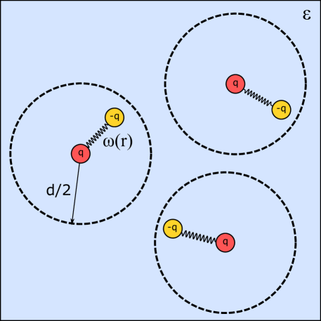
Figure 3: Schematic representation of a salt-free solution of zwitterions with a hard core.

A point-like charge $q$ is placed at the center of each hard sphere with a diameter $d$ and an oppositely charged site $-q$ is grafted to the center of the sphere. Let me also assume that the charged sites $\pm q$ are separated by a fluctuating distance described by a probability distribution function $\omega(\mathbb{r})$. Let me assume also that the charged site $-q$ is a phantom one, so that it can penetrate inside the hard cores of molecules. The screening function of such a system can be written in the following form (for details, see Appendix II)

$$\varkappa^{2}(\mathbb{k})=\frac{8\pi nq^{2}}{\varepsilon k_{B}T}\left(1-\omega(\mathbb{k})\right)\left(1+\frac{1}{2}\left(S(\mathbb{k})-1\right)\left(1-\omega(\mathbb{k})\right)\right),$$ (59)

where

$$S(\mathbb{k})=1+nh(\mathbb{k})$$ (60)

is the structure factor of the hard spheres system expressed via the Fourier-image $h(\mathbb{k})$ of the pair correlation function Hansen and McDonald (1990). The electrostatic free energy is determined by eq. (40) with screening function (59). We would like to note that the structure factor (60) of hard spheres system does not determine the total structure factor of zwitterions. The total structure factor, taking into account dipole-dipole interactions, can behave different from the structure factor of hard spheres. Further, using the $"$mean-field$"$ approximation $S(\mathbb{k})\approx S(0)=nk_{B}T\chi_{T}=z_{0}$, where $\chi_{T}$ is the isothermal compressibility of the hard spheres system, and using the characteristic function $\omega(\mathbb{k})=(1+k^{2}l^{2}/6)^{-1}$, one can obtain an analytical expression for the electrostatic free energy of the dipolar hard spheres Budkov and Kolesnikov (2020). I do not provide a rather cumbersome expression for electrostatic free energy here and write only the limiting regimes following from it

$$\frac{F_{el}}{Vk_{B}T}=\begin{cases}-\frac{\sqrt{6}\pi q^{4}l}{3\left(\varepsilon k_{B}T\right)^{2}}n^{2}\left(1-\frac{3}{4}\alpha+\frac{5\alpha^{2}}{32}\right),\leavevmode\nobreak\ y_{d}\ll 1\,\\ -\frac{1}{12\pi r_{D}^{3}}\left(1-\frac{3}{2}\alpha-3(1-e^{\alpha/4})\right),\leavevmode\nobreak\ y_{d}\gg 1,\end{cases}$$ (61)

where $\alpha=1-z_{0}$. In the Percus-Yevick Hansen and McDonald (1990); Gray and Gubbins (1984) approximation I get

$$\alpha=\frac{\eta(4-\eta)(2+\eta^{2})}{(1+2\eta)^{2}},$$ (62)

where $\eta=\pi d^{3}n/6$ is the packing fraction of the hard spheres Hansen and McDonald (1990). Using limiting regimes (61), one can construct the approximate expression Budkov and Kolesnikov (2020) which quite well reproduces the electrostatic free energy for all values of $y_{d}$ and $0<\alpha<1$:

$$F_{el}\approx-\frac{Vk_{B}T}{l^{3}}\left(1-\frac{3}{4}\alpha\right)\sigma(y_{d}),$$ (63)

As one can see from the comparison of eqs. (63) and (42), accounting for the excluded volume of the zwitterions reduces the electrostatic contribution to the total free energy. The latter can be explained by the fact that the hard core of the molecules makes their overlapping impossible, thus, decreasing the electrostatic interactions.

The adopted $"$mean-field$"$ approximation $S(\mathbb{k})\approx S(0)$ would be valid when the contribution of $k\ll 2\pi/d$ makes dominant contribution in integrals over $\mathbb{k}$, which means that the interaction between molecules at distances much larger than $d$ is important. However, for the systems of high molecular concentration this approximation is not valid. In this case, it is necessary to integrate numerically over $\mathbb{k}$, using analytical expression for structure factor of hard sphere systems within the Percus-Yiewick approximation Santos (2016). Moreover, we would like to note that RPA is valid at sufficiently small electrostatic interactions between charged particles Naji et al. (2013). Only in this case we can use the hard spheres fluid as a reference system, considering the electrostatic contribution as perturbation.

III Solutions of multipolar molecules

In the previous section, I considered the general statistical field theory of salt solutions of zwitterions, which might be used for describing the thermodynamic properties of real ion-molecular solutions, such as proteins and betaines, whose molecules possess large dipole moments. However, there is a wide class of macromolecules, acquiring a complex electric structure in solvent media, which cannot be reduced to two oppositely charge centers – a dipolar structure. As it was already mentioned in the introductory section, the most natural generalization of the dipolar structure is the structure of a $"$star$"$, i.e., when the $"$central$"$ charge $q$ is placed at the center of the molecule, surrounded by $"$peripheral$"$ charges $q_{\alpha}$ ($\alpha=1,...,m$). The positions of the peripheral charges relative to the central charge are fixed or fluctuating ones. Each molecule is assumed to be electrically neutral, so that the neutrality condition $q+\sum_{\alpha}q_{\alpha}=0$ is fulfilled. As I have already mentioned in the Introduction, such multipolar configurations could be realized for macromolecular systems, such as polyelectrolyte brushes and stars, complex colloids, and metal-organic complexes. Despite the fact that there is a wide range of possible applications, up to now, there have been no attempts to develop the statistical theories of salt solutions of multipolar molecules Budkov (2019a). In this section, I would like to consider the FT model of salt solutions of neutral molecules, possessing a multipolar electric structure. As in the case of the above described solutions of zwitterionic molecules, I assume that the ions with total numbers $N_{i}$ and valencies $z_{i}$ ($i=1,...,s$) are dissolved in a solvent medium along with multipolar molecules. As in the previous section, the global neutrality condition $\sum_{i}z_{i}N_{i}=0$ is fulfilled and the solvent is supposed to be a continuous dielectric medium with a constant permittivity $\varepsilon$. I assume that each peripheral charge $q_{\alpha}$ is separated from the central charge $q$ by the fluctuating distance $\mathbb{\xi}_{\alpha}$, described by the distribution function $\omega_{\alpha}(\mathbb{\xi}_{\alpha})$ ($\alpha=1,..,m$). I also assume that the solution is rather dilute, the excluded volume interactions between all the species can be neglected. The effects of excluded volume interactions will be discussed at the end of this section.

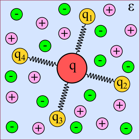
Figure 4: Schematic representation of the multipolar molecule surrounded by salt ions in a dielectric solvent medium.

Taking into account all the model assumptions, one can write the configuration integral of the system in the form

$$Q=\int d\Gamma_{s}\int d\Gamma_{h}\exp\left[-\beta H_{int}\right],$$ (64)

where

$$\int d\Gamma_{h}(\cdot)=\int\dots\int\prod\limits_{j=1}^{N}d\Gamma_{j}(\cdot)$$ (65)

is the integration measure over the configurations $\Gamma_{j}$ of the $"$hairy$"$ multipolar molecules

$$\int d\Gamma_{j}(\cdot)=\int\frac{d\mathbb{R}_{j}}{V}\int\dots\int\prod\limits_{\alpha=1}^{m}d\mathbb{\xi}_{j}^{(\alpha)}\omega_{\alpha}\left(\xi_{j}^{(\alpha)}\right)(\cdot),$$ (66)

where $\mathbb{\xi}_{j}^{(\alpha)}$ are the displacement vectors of the peripheral charges relative to the positions $\mathbb{R}_{j}$ of the central charges. The measure of integration over the positions of the salt ions is determined by eq. (4). The total potential energy of the electrostatic interactions is

$$H_{int}=\frac{1}{2}\int d\mathbb{r}\int d\mathbb{r}^{\prime}\hat{\rho}(\mathbb{r})G_{0}(\mathbb{r}-\mathbb{r}^{\prime})\hat{\rho}(\mathbb{r}^{\prime})=\frac{1}{2}\left(\hat{\rho}G_{0}\hat{\rho}\right),$$ (67)

where

$$\hat{\rho}(\mathbb{r})=\hat{\rho}_{h}(\mathbb{r})+\hat{\rho}_{i}(\mathbb{r})+\rho_{ext}(\mathbb{r})$$ (68)

is the total charge density of the system, where

$$\hat{\rho}_{h}(\mathbb{r})=\sum\limits_{\alpha=1}^{m}q_{\alpha}\sum\limits_{j=1}^{N}\left(\delta\left(\mathbb{r}-\mathbb{R}_{j}-\mathbb{\xi}_{j}^{(\alpha)}\right)-\delta\left(\mathbb{r}-\mathbb{R}_{j}\right)\right)$$ (69)

is the local charge density of the multipolar molecules and $\hat{\rho}_{i}(\mathbb{r})$ is determined by eq. (8). Using HS transformation (9), I arrive in the thermodynamic limit at

$$Q=\int\frac{\mathcal{D}\varphi}{C}\exp\left[-S[\varphi]\right],$$ (70)

where

$$S[\varphi]=\frac{\beta}{2}(\varphi G_{0}^{-1}\varphi)-i\beta(\rho_{ext}\varphi)-W[\varphi]$$ (71)

with

$$W[\varphi]=n\int d\mathbb{R}\left<e^{i\beta\sum\limits_{\alpha=1}^{m}q_{\alpha}(\varphi(\mathbb{R}+\mathbb{\xi}_{\alpha})-\varphi(\mathbb{R}))}-1\right>_{\xi}+\sum\limits_{j=1}^{s}c_{j}\int d\mathbb{r}(e^{i\beta z_{j}e\varphi(\mathbb{r})}-1).$$ (72)

Note that in the latter equation I introduced notation for averaging over the configurations of the peripheral charges

$$\left<(\cdot)\right>_{\xi}=\int d\mathbb{\xi}_{1}\dots\int d\mathbb{\xi}_{m}\prod\limits_{\alpha=1}^{m}\omega_{\alpha}(\mathbb{\xi}_{\alpha})(\cdot).$$ (73)

Oscillations of the electrostatic potential. The self-consistent field equation for the salt solution of the multipolar molecules takes the form Budkov (2019a)

$$\Delta\psi(\mathbb{r})=-\frac{4\pi}{\varepsilon}\left(\rho_{ext}(\mathbb{r})+\bar{\rho}_{i}(\mathbb{r})+\bar{\rho}_{h}(\mathbb{r})\right),$$ (74)

where $\bar{\rho}_{i}(\mathbb{r})$ is the average charge density of the ions, determined by eq. (54) and

$$\bar{\rho}_{h}(\mathbb{r})=n\sum\limits_{\gamma=1}^{m}q_{\gamma}\left<e^{-\beta\sum\limits_{\alpha=1}^{m}q_{\alpha}\left(\psi(\mathbb{r}+\mathbb{\xi}_{\alpha}-\mathbb{\xi}_{\gamma})-\psi(\mathbb{r}-\mathbb{\xi}_{\gamma})\right)}-e^{-\beta\sum\limits_{\alpha=1}^{m}q_{\alpha}\left(\psi(\mathbb{r}+\mathbb{\xi}_{\alpha})-\psi(\mathbb{r})\right)}\right>_{\xi}$$ (75)

is the average charge density of the multipolar hairy molecules.

In the linear approximation, eq. (74) yields the following expression for the electrostatic potential of the external charges

$$\psi(\mathbb{r})=\frac{4\pi}{\varepsilon}\int\frac{d\mathbb{k}}{(2\pi)^{3}}\frac{\tilde{\rho}_{ext}(\mathbb{k})e^{i\mathbb{k}\mathbb{r}}}{k^{2}+\varkappa^{2}(\mathbb{k})},$$ (76)

with the following screening function

$$\varkappa^{2}(\mathbb{k})=\kappa_{s}^{2}+\frac{4\pi n}{\varepsilon k_{B}T}\left(|q(\mathbb{k})|^{2}+\sum\limits_{\alpha=1}^{m}q_{\alpha}^{2}(1-|\omega_{\alpha}(\mathbb{k})|^{2})\right),$$ (77)

and the Fourier-image of the density of the external charges $\tilde{\rho}_{ext}(\mathbb{k})$. I have introduced the characteristic functions

$$\omega_{\alpha}(\mathbb{k})=\int d\mathbb{r}\omega_{\alpha}(\mathbb{r})e^{-i\mathbb{k}\mathbb{r}}$$ (78)

and the auxiliary function

$$q(\mathbb{k})=\sum_{\alpha=1}^{m}q_{\alpha}(1-\omega_{\alpha}(\mathbb{k})).$$ (79)

Note that for $m=1$, screening function (77) transforms into the above written screening function (19) for the zwitterionic molecules. Note also that within the linear approximation (76) the electrostatic correlations between peripheral charges within one multipolar molecule are not taken into account. The latter can be justified by sufficiently small electrostatic interactions which unable to disturb strongly the configuration of multipolar molecules.

Using eq. (76), one can analyse the behavior of the potential of the point-like test ion $q_{0}$, immersed in a salt solution of multipolar particles, at long distances. I assume that all the peripheral charges $q_{\alpha}$ have the same sign and the distribution functions are spherically symmetric ones, i.e. $\omega_{\alpha}(\mathbb{r})=\omega_{\alpha}(|\mathbb{r}|)$. In that case the characteristic functions can be expanded into a power series near $\mathbb{k}=0$, so that $\omega_{\alpha}(\mathbb{k})=1-k^{2}\left<\xi_{\alpha}^{2}\right>/2!+k^{4}\left<\xi_{\alpha}^{4}\right>/4!+O(k^{6})$. Placing the test ion at the origin and taking into account that $\rho_{ext}(\mathbb{r})=q_{0}\delta(\mathbb{r})$, I obtain

$$\psi(\mathbb{r})\simeq\frac{4\pi q_{0}}{\varepsilon_{b}}\int\frac{d\mathbb{k}}{(2\pi)^{3}}\frac{e^{i\mathbb{k}\mathbb{r}}}{k^{2}+\tilde{\kappa}_{s}^{2}+L_{Q}^{2}k^{4}},$$ (80)

where $\varepsilon_{b}=\varepsilon+4\pi n\sum_{\alpha}q_{\alpha}^{2}\left<\xi_{\alpha}^{2}\right>/(k_{B}T)$ is the bulk dielectric permittivity of the solution, taking into account the dielectric effect of the multipolar molecules, $\tilde{\kappa}_{s}=(8\pi e^{2}I/k_{B}T\varepsilon_{b})^{1/2}$ is the inverse Debye length of the salt ions in the dielectric medium with the permittivity $\varepsilon_{b}$. The $"$quadrupolar$"$ length $L_{Q}$ Budkov (2019a); Slavchov (2014) is determined by the relation

$$L_{Q}^{2}=\frac{\pi n}{\varepsilon_{b}k_{B}T}\sum\limits_{\alpha,\gamma}q_{\alpha}q_{\gamma}\left(\left<\xi_{\alpha}^{2}\right>\left<\xi_{\gamma}^{2}\right>\left(1-\delta_{\alpha\gamma}\right)-\frac{1}{3}\delta_{\alpha\gamma}\left<\xi_{\alpha}^{4}\right>\right),$$ (81)

where $\delta_{\alpha\gamma}$ is the Kronecker symbol. The quadrupolar length is positive at sufficiently large number $m$ of the identical peripheral charges $q_{\alpha}=-q/m$ with $\left<\xi_{\alpha}^{2}\right>=l^{2}/6$. In this case of pure quadrupolar molecules, the quadrupolar length is determined by the following expression Budkov (2019a)

$$L_{Q}^{2}\simeq\frac{\pi q^{2}nl^{4}}{9\varepsilon k_{B}T}.$$ (82)

Therefore, for the case of quadrupolar molecules calculation of integral in eq. (80) yields Budkov (2019a)

$$\psi(\mathbb{r})=\frac{q_{0}}{\varepsilon_{b}r}\times\begin{cases}\frac{\exp\left(-\kappa_{-}r\right)-\exp\left(-\kappa_{+}r\right)}{\sqrt{1-4\tilde{\kappa}_{s}^{2}L_{Q}^{2}}},&\tilde{\kappa}_{s}L_{Q}<\frac{1}{2}\\ \frac{r}{\sqrt{2}L_{Q}}\exp\left(-\frac{r}{\sqrt{2}L_{Q}}\right),&\tilde{\kappa}_{s}L_{Q}=\frac{1}{2}\\ \frac{\exp\left(-\kappa_{0}r\right)}{\sqrt{4\tilde{\kappa}_{s}^{2}L_{Q}^{2}-1}}\sin\left(\frac{r}{\lambda}\right),&\tilde{\kappa}_{s}L_{Q}>\frac{1}{2},\end{cases}$$ (83)

where $r=|\mathbb{r}|$ and the following short-hand notations

$$\kappa_{\pm}=\frac{\left(1\pm\sqrt{1-4\tilde{\kappa}_{s}^{2}L_{Q}^{2}}\right)^{1/2}}{\sqrt{2}L_{Q}},\leavevmode\nobreak\ \leavevmode\nobreak\ \kappa_{0}=\tilde{\kappa}_{s}\sqrt{1+1/(2\tilde{\kappa}_{s}L_{Q})},$$ (84)

$$\lambda=\frac{1}{\tilde{\kappa}_{s}\sqrt{1-1/(2\tilde{\kappa}_{s}L_{Q})}}$$ (85)

are introduced. As is seen, the electrostatic potential behaves at long distances in two qualitatively different manners. If the quadrupolar length is less than half of the Debye length, the potential monotonically decreases at long distances. However, in the case when the quadrupolar length exceeds half of the Debye length, the potential damps with oscillations, characterized by a certain wavelength $\lambda$ and a decrement $\kappa_{0}$. Such an asymptotic behavior of the potential was originally discovered by Slavchov Slavchov (2014) in the framework of the pure phenomenological theory. I would like to note that the oscillations of the electrostatic potential is a peculiarity of the ion-quadrupole media. It is also interesting to note that analogous oscillations of the electrostatic potential can be observed in ionic liquids at electrified interfaces (so-called overscreening) Bazant, Storey, and Kornyshev (2011); Fedorov and Kornyshev (2014). Recently, using the idea that ions in ionic liquids can form electrically neutral quadrupolar clusters Feng et al. (2019); Coles et al. (2019), Avni et al. Avni, Adar, and Andelman (2020) proposed a possible mechanism of the overscreening effect. I would like to stress that oscillations of the mean-force electrostatic potential in ionic media containing quadrupolar clusters is a new fundamental effect taking place in different ion-molecular systems. In terms of statistical mechanics, the obtained crossover from a monotonic decrease in the mean-force electrostatic potential to its oscillating decrease is related to exceeding of the so-called Fisher-Widom line Fisher and Widom (1969); Stopper et al. (2019) on the phase diagram of the solution. Thus, the Fisher-Widom line for the ionic component of the solution is determined by the equation $\tilde{\kappa}_{s}L_{Q}=1/2$. The length $\kappa_{0}^{-1}$ characterizes the decay of the correlations of ionic concentration fluctuations, and is analogous to Ornstein-Zernike correlation length Barrat and Hansen (2003), while $\lambda$ is a measure of the $"$periodicity$"$ of positive ion-rich and negative ion-rich domains. The analogous charge periodicity is realized in salt solutions of weak polyelectrolytes Borue and Erukhimovich (1988). Note that similar periodicity of oil-rich and water-rich domains can be observed in microemulsions Barrat and Hansen (2003). I would like to note also that given analysis of electrostatic potential is valid only in case when $\tilde{\kappa}_{s}L_{Q}\sim 1$. In case when $\tilde{\kappa}_{s}L_{Q}\gg 1$ the low-k expansion of the screening function is not valid, and, thereby, higher order terms must be included.

Electrostatic free energy. The electrostatic free energy of the bulk solution is determined by eq. (40) with screening function (77). Now let me consider the case of identical peripheral charges $q_{\alpha}=-q/m$ with the same spherically symmetric distribution functions $\omega_{\alpha}(\mathbb{r})=\omega(|\mathbb{r}|)$. In this case, the screening function takes the form

$$\varkappa^{2}(\mathbb{k})=\kappa_{s}^{2}+\frac{4\pi q^{2}n(m+1)}{\varepsilon k_{B}Tm}(1-\omega(\mathbb{k}))\left(1-\frac{m-1}{m+1}\omega(\mathbb{k})\right).$$ (86)

For the case of dipolar molecules ($m=1$), eq. (86) yields the earlier obtained eq. (19). It is interesting to consider another limiting case $m\gg 1$, when the peripheral charges form a continuous charged cloud surrounding the central charge. In this case, the screening function takes the following form

$$\varkappa^{2}(\mathbb{k})\simeq\kappa_{s}^{2}+\frac{4\pi q^{2}n}{\varepsilon k_{B}T}(1-\omega(\mathbb{k}))^{2}.$$ (87)

For the model distribution function determined by characteristic function (21), one can obtain an analytical expression for the electrostatic free energy for the salt-free solution ($\kappa_{s}=0$), i.e.

$$F_{el}=-\frac{Vk_{B}T}{l^{3}}s(y),$$ (88)

where $s(y)=\sqrt{6}\pi^{-1}\left((1+y)\sqrt{1+y/4}-{9y}/{8}-1\right)$, $y=2\pi q^{2}l^{2}n/(3\varepsilon k_{B}T)=\kappa^{2}l^{2}/6$, and $\kappa=(4\pi q^{2}n/\varepsilon k_{B}T)^{1/2}$ is the inverse Debye length, attributed to the central charges. It is interesting to analyse the limiting cases, following from eq. (88). Thus, I have

$$\frac{F_{el}}{Vk_{B}T}=\begin{cases}-\frac{5\sqrt{6}\pi q^{4}l}{96\left(\varepsilon k_{B}T\right)^{2}}n^{2},&y\ll 1\\ -\frac{\kappa^{3}}{12\pi},&y\gg 1.\end{cases}$$ (89)

The first regime determines the case, when the effective size of charged cloud $l$ is much less than the Debye length $\kappa^{-1}$. In this case, the effective interactions of the multipolar molecules manifest themselves as the effective Van der Waals interaction – Kirkwood-Shumaker attractive interaction Kirkwood and Shumaker (1952); Adžić and Podgornik (2015); Avni, Andelman, and Podgornik (2019), which is caused by the spatial fluctuations of the charged clouds of the molecules. In the opposite case, the electrostatic free energy is described by the DH limiting law. In this case, a salt-free solution can be described by the one-component plasma model (see papers Brilliantov (1998b); Ortner (1999) and report Levin (2002)). Indeed, in the latter case the central charges are immersed in the background of collectivized charged clouds. In the regime $y\ll 1$, one can obtain Budkov (2019a)

$$\frac{F_{el}}{Vk_{B}T}=-\frac{\kappa_{s}^{3}}{12\pi}-\frac{\sqrt{6}\pi q^{2}n}{\varepsilon k_{B}Tl}h_{1}(y_{s})-\frac{\sqrt{6}\pi q^{4}ln^{2}}{96(\varepsilon k_{B}T)^{2}}h_{2}(y_{s})+O(n^{3}),$$ (90)

where $y_{s}=\kappa_{s}^{2}l^{2}/6$ and the following functions are introduced

$$h_{1}(y_{s})=\frac{y_{s}(1+2\sqrt{y_{s}})}{(1+\sqrt{y_{s}})^{2}},\leavevmode\nobreak\ h_{2}(y_{s})=\frac{40y_{s}^{3/2}+8y_{s}^{2}+48y_{s}+25\sqrt{y_{s}}+5}{(1+\sqrt{y_{s}})^{5}}.$$ (91)

In the regime when $y_{s}\gg 1$ and $y\gg 1$, I obtain

$$\frac{F_{el}}{Vk_{B}T}=-\frac{(\kappa^{2}+\kappa_{s}^{2})^{3/2}}{12\pi}.$$ (92)

The latter expression determines the DH limiting law for the one-component plasma in the presence of salt ions.

Multipolar molecules with a hard core. Now I would like to demonstrate how one can take into account the excluded volume interactions between the multipolar molecules. For this purpose, let me assume that the central charges are placed at the centers of hard spheres with a diameter $d$. Let me also consider the peripheral charges as phantom ones, which can penetrate freely inside the hard cores of multipolar molecules. For simplicity, I consider only the case of salt-free solution of the multipolar molecules. . The screening function for this case takes the following form (for details, see Appendix II)

$$\varkappa^{2}(\mathbb{k})=\frac{4\pi n}{\varepsilon k_{B}T}\left(|q(\mathbb{k})|^{2}S(\mathbb{k})+\sum\limits_{\alpha=1}^{m}q_{\alpha}^{2}(1-|\omega_{\alpha}(\mathbb{k})|^{2})\right),$$ (93)

where the function $q(\mathbb{k})$ is determined by eq. (79) and $S(\mathbb{k})$ is the structure factor of the hard spheres system determined above. The electrostatic free energy is determined by eq. (40) with screening function (93). Considering only the case of identical peripheral charges $q_{\alpha}=-q/m$ and the case of $m\gg 1$, one can get

$$\varkappa^{2}(\mathbb{k})\simeq\frac{4\pi q^{2}n}{\varepsilon k_{B}T}(1-\omega(\mathbb{k}))^{2}S(\mathbb{k}).$$ (94)

Further, using the discussed in section I $"$mean-field$"$ approximation $S(\mathbb{k})\approx S(0)=nk_{B}T\chi_{T}=z_{0}$, where $\chi_{T}$ is the isothermal compressibility of the hard spheres system, I arrive at the following expression for the electrostatic free energy

$$F_{el}=-\frac{Vk_{B}T}{l^{3}}s(\tilde{y}),$$ (95)

where $\tilde{y}=yz_{0}$ and the auxiliary function $s(y)$ has been determined above. The limiting regimes resulting from eq. (95) are

$$\frac{F_{el}}{Vk_{B}T}=\begin{cases}-\frac{5\sqrt{6}\pi q^{4}l}{96\left(\varepsilon k_{B}T\right)^{2}}z_{0}^{2}n^{2},&y\ll 1\\ -\frac{\kappa^{3}}{12\pi}z_{0}^{3/2},&y\gg 1.\end{cases}$$ (96)

In the Percus-Yevick approximation Hansen and McDonald (1990) the compressibility factor is determined by the expression Hansen and McDonald (1990) $z_{0}=(1-\eta)^{4}/(1+2\eta)^{2}<1$. Therefore, as in the case of zwitterions with a hard core, accounting for the excluded volume correlations of the multipolar molecules reduces the absolute value of electrostatic contribution to the total free energy of solution.

IV Conclusions and future prospects

In this paper, in the context of the modern statistical physics of ion-molecular systems, I have outlined my recent developments in the statistical field theory of salt solutions of zwitterions and multipolar molecules. I have formulated a general field theoretic formalism, going beyond the standard simple fluids field theory paradigm. The presented findings allow taking into account the complex internal electric structure of zwitterionic and multipolar molecules in the salt solution media. I have demonstrated how the formulated formalism can be applied to the calculations of various thermodynamic properties of the salt solutions of zwitterions and multipolar molecules. I believe that this formalism can be used in future as a theoretical background, making it possible to properly describe the electrostatic interactions within the theoretical models of ion-molecular systems, such as salt solutions of metal-organic complexes, complex colloids, phospholipids, betaines, proteins, etc.

V Appendix I: Electrostatic free energy of a solution of multipolar molecules

In this Appendix, I would like to describe the process of deriving the expression for the electrostatic free energy of the bulk salt solution of the multipolar molecules within the RPA. As it was already mentioned in the main text, the configuration integral of a solution of multipolar molecules within the RPA takes the following general form

$$Q\approx\exp\left\{-S[i\psi]+\frac{1}{2}tr\left(\ln\mathcal{G}-\ln G_{0}\right)\right\},$$ (97)

where the symbol $tr(..)$ denotes a trace of the integral operator $A$ with the kernel $A(\mathbb{r},\mathbb{r}^{\prime})$ in accordance with the following definition

$$tr(A)=\int d\mathbb{r}A(\mathbb{r},\mathbb{r}).$$ (98)

The inverse Green function can be written as follows

$$\mathcal{G}^{-1}(\mathbb{r},\mathbb{r}^{\prime}|\psi)=k_{B}T\frac{\delta^{2}S[i\psi]}{\delta\varphi(\mathbb{r})\delta\varphi(\mathbb{r}^{\prime})}=G_{0}^{-1}(\mathbb{r},\mathbb{r}^{\prime})+\mathcal{R}_{i}(\mathbb{r},\mathbb{r}^{\prime}|\psi)+\mathcal{R}_{h}(\mathbb{r},\mathbb{r}^{\prime}|\psi)$$ (99)

where

$$\mathcal{R}_{i}(\mathbb{r},\mathbb{r}^{\prime}|\psi)=\beta e^{2}\sum\limits_{j=1}^{s}z_{j}^{2}c_{j}e^{-\beta z_{j}e\psi(\mathbb{r})}\delta(\mathbb{r}-\mathbb{r}^{\prime}),$$ (100)

and

$$\mathcal{R}_{h}(\mathbb{r},\mathbb{r}^{\prime}|\psi)=\beta n\sum\limits_{\delta,\gamma}q_{\delta}q_{\gamma}\left<e^{-\beta\sum\limits_{\alpha=1}^{m}q_{\alpha}\left(\psi(\mathbb{r}+\mathbb{\xi}_{\alpha}-\mathbb{\xi}_{\gamma})-\psi(\mathbb{r}-\mathbb{\xi}_{\gamma})\right)}\left(\delta(\mathbb{r}-\mathbb{r}^{\prime}+\mathbb{\xi}_{\delta}-\mathbb{\xi}_{\gamma})-\delta(\mathbb{r}-\mathbb{r}^{\prime}-\mathbb{\xi}_{\gamma})\right)\right>_{\xi}$$

$$-\beta n\sum\limits_{\delta,\gamma}q_{\delta}q_{\gamma}\left<e^{-\beta\sum\limits_{\alpha=1}^{m}q_{\alpha}\left(\psi(\mathbb{r}+\mathbb{\xi}_{\alpha})-\psi(\mathbb{r})\right)}\left(\delta\left(\mathbb{r}-\mathbb{r}^{\prime}+\mathbb{\xi}_{\delta}\right)-\delta\left(\mathbb{r}-\mathbb{r}^{\prime}\right)\right)\right>_{\xi}.$$ (101)

I would like to note that for the case of dipolar molecules ($m=1$) eq. (99) transforms into eq. (38) written above. In the absence of the external charges (i.e., $\rho_{ext}(\mathbb{r})=0$), the self-consistent field potential $\psi(\mathbb{r})=0$, so that the mean-field contribution $F_{el}^{(MF)}=k_{B}TS[0]=0$. Therefore, the inverse Green function takes the following simplified form:

$$\mathcal{G}^{-1}(\mathbb{r},\mathbb{r}^{\prime}|0)=G^{-1}(\mathbb{r},\mathbb{r}^{\prime})=G_{0}^{-1}(\mathbb{r},\mathbb{r}^{\prime})+R_{i}(\mathbb{r},\mathbb{r}^{\prime})+R_{h}(\mathbb{r},\mathbb{r}^{\prime})$$

where the following kernels

$$R_{i}(\mathbb{r},\mathbb{r}^{\prime})=\mathcal{R}_{i}(\mathbb{r},\mathbb{r}^{\prime}|0)=2\beta Ie^{2}\delta(\mathbb{r}-\mathbb{r}^{\prime}),$$ (102)

$$R_{h}(\mathbb{r},\mathbb{r}^{\prime})=\mathcal{R}_{h}(\mathbb{r},\mathbb{r}^{\prime}|0)=\beta n\sum\limits_{\delta,\gamma}q_{\delta}q_{\gamma}\left<\delta\left(\mathbb{r}-\mathbb{r}^{\prime}+\mathbb{\xi}_{\delta}-\mathbb{\xi}_{\gamma}\right)-2\delta\left(\mathbb{r}-\mathbb{r}^{\prime}-\mathbb{\xi}_{\gamma}\right)+\delta\left(\mathbb{r}-\mathbb{r}^{\prime}\right)\right>_{\xi}$$ (103)

are introduced; $I$ is the ionic strength of the solution determined in the main text.

The electrostatic free energy, thus, is determined by

$$F_{el}\approx\frac{k_{B}T}{2}tr\left(\ln G_{0}-\ln G\right)=\frac{Vk_{B}T}{2}\int\frac{d\mathbb{k}}{(2\pi)^{3}}\ln\frac{G_{0}(\mathbb{k})}{G(\mathbb{k})},$$ (104)

where $G_{0}(\mathbb{k})=4\pi/(\varepsilon k^{2})$ and $G(\mathbb{k})=4\pi/(\varepsilon(k^{2}+\varkappa^{2}(\mathbb{k})))$ are the Fourier-images of the Green functions; the screening function $\varkappa^{2}(\mathbb{k})$ is determined by eq. (77).

Now let me derive eq. (104). Thus, I have

$$tr\left(\ln G_{0}-\ln G\right)=tr\ln(G^{-1}G_{0})=tr\ln((G_{0}^{-1}+R)G_{0})=tr\ln(\mathbb{I}+A),$$ (105)

where $\mathbb{I}$ is the identity operator and $A=RG_{0}$ with $R=R_{i}+R_{h}$. Therefore, I obtain

$$tr\ln(\mathbb{I}+A)=\sum\limits_{n=1}^{\infty}\frac{(-1)^{n+1}}{n}tr(A^{n}).$$ (106)

In accordance with the above-mentioned definition (98), I can write

$$tr(A^{n})=\int d\mathbb{r}(A^{n})(\mathbb{r},\mathbb{r}),$$ (107)

where

$$(A^{n})(\mathbb{r},\mathbb{r}^{\prime})=\int d\mathbb{r}_{1}..\int d\mathbb{r}_{n-1}A(\mathbb{r}-\mathbb{r}_{1})A(\mathbb{r}_{1}-\mathbb{r}_{2})...A(\mathbb{r}_{n-2}-\mathbb{r}_{n-1})A(\mathbb{r}_{n-1}-\mathbb{r}^{\prime})$$

$$=\int\frac{d\mathbb{k}}{(2\pi)^{3}}e^{i\mathbb{k}(\mathbb{r}-\mathbb{r}^{\prime})}\tilde{A}^{n}(\mathbb{k}),$$ (108)

where

$$\tilde{A}(\mathbb{k})=\int d\mathbb{r}e^{-i\mathbb{k}\mathbb{r}}A(\mathbb{r})$$ (109)

is the Fourier-image of the function $A(\mathbb{r})$. Therefore, I obtain

$$tr(A^{n})=V\int\frac{d\mathbb{k}}{(2\pi)^{3}}\tilde{A}^{n}(\mathbb{k}),$$ (110)

where I take into account that $\int d\mathbb{r}=V$. Further, using eq. (106), I arrive at the following equality

$$tr\ln(\mathbb{I}+A)=V\int\frac{d\mathbb{k}}{(2\pi)^{3}}\ln\left(1+\tilde{A}(\mathbb{k})\right).$$ (111)

Therefore, taking into account that $\tilde{A}(\mathbb{k})=\tilde{R}(\mathbb{k})G_{0}(\mathbb{k})=\varkappa^{2}(\mathbb{k})/k^{2}$, I finally obtain

$$F_{el}=\frac{Vk_{B}T}{2}\int\frac{d\mathbb{k}}{(2\pi)^{3}}\ln\left(1+\frac{\varkappa^{2}(\mathbb{k})}{k^{2}}\right)=\frac{Vk_{B}T}{2}\int\frac{d\mathbb{k}}{(2\pi)^{3}}\ln\frac{G_{0}(\mathbb{k})}{G(\mathbb{k})},$$ (112)

where I take into account that

$$\tilde{R}(\mathbb{k})=\tilde{R}_{i}(\mathbb{k})+\tilde{R}_{h}(\mathbb{k})=2\beta I+\beta n\left(|q(\mathbb{k})|^{2}+\sum\limits_{\alpha=1}^{m}q_{\alpha}^{2}(1-|\omega_{\alpha}(\mathbb{k})|^{2})\right).$$ (113)

Subtracting the electrostatic self-energy $E_{self}=V/(2(2\pi)^{3})\int{d\mathbb{k}}\varkappa^{2}(\mathbb{k})/k^{2}$ of the particles, I arrive at eq. (40).

VI Appendix II: Derivation of electrostatic free energy of a salt-free solution of multipolar molecules with excluded volume interactions

In this appendix, I consider the derivation of the electrostatic free energy of a salt-free solution of multipolar molecules taking into account the excluded volume interactions between them. As it was already mentioned in the main text, the central charge $q$ is placed at the center of a hard sphere with a diameter $d$, whereas the peripheral charges $q_{\alpha}$ ($\alpha=1,...,m$) are the phantom ones which can freely penetrate inside the hard core. Therefore, the configuration integral of such a system can be written as follows

$$Q=\int d\Gamma_{h}\exp\left[-\beta H_{hc}-\beta H_{el}\right],$$ (114)

where the integration over the configurations of the multipolar molecules is performed in accordance with definitions (65) and (66). The first term in the integrand exponent describes the contribution of the excluded volume interactions between the multipolar molecules, i.e.

$$H_{hc}=\frac{1}{2}\sum\limits_{i\neq j}U_{hc}(\mathbb{R}_{i}-\mathbb{R}_{j}),$$ (115)

where

$$U_{hc}(\mathbb{r})=\begin{cases}0,|\mathbb{r}|>0\,\\ \infty,|\mathbb{r}|\leq 0,\end{cases}$$ (116)

is the hard core potential. The second term describes the potential energy of electrostatic interactions of the multipolar molecules, i.e.

$$H_{el}=\frac{1}{2}\left(\hat{\rho}_{h}G_{0}\hat{\rho}_{h}\right)=\frac{1}{2}\int d\mathbb{r}\int d\mathbb{r}^{\prime}\hat{\rho}_{h}(\mathbb{r})G_{0}(\mathbb{r}-\mathbb{r}^{\prime})\hat{\rho}_{h}(\mathbb{r}^{\prime}),$$ (117)

where $\hat{\rho}_{h}(\mathbb{r})$ is the microscopic charge density of multipolar molecules which is determined by eq. (69). Further, using the hard spheres system as a reference system, I can recast the configuration integral in the thermodynamic perturbation theory fashion, i.e.

$$Q=Q_{hs}\left<\exp\left[-\frac{1}{2}\left(\hat{\rho}_{h}G_{0}\hat{\rho}_{h}\right)\right]\right>,$$ (118)

where

$$Q_{hs}=\int d\Gamma_{h}\exp\left[-\beta H_{hc}\right]$$ (119)

is the configuration integral of the reference system and the notation

$$\left<(...)\right>=\frac{1}{Q_{hs}}\int d\Gamma_{h}\exp\left[-\beta H_{hc}\right](...)$$ (120)

denotes the averaging over the microstates of the reference system. Using the Hubbard-Stratonovich transformation, I arrive at the following representation of the configuration integral

$$Q=Q_{hs}\int\frac{\mathcal{D}\varphi}{C}\exp\left[-\frac{\beta}{2}(\varphi G_{0}^{-1}\varphi)\right]\left<\exp\left[i\beta(\hat{\rho}_{h}\varphi)\right]\right>.$$ (121)

The cumulant expansion Kubo (1962) gives

$$\left<\exp\left[i\beta(\hat{\rho}_{h}\varphi)\right]\right>=\exp\left[i\beta(\left<\hat{\rho}_{h}\right>\varphi)-\frac{\beta^{2}}{2}\left(\varphi\mathcal{K}\varphi\right)+...\right],$$ (122)

where

$$\mathcal{K}(\mathbb{r}-\mathbb{r}^{\prime})=\left<\hat{\rho}_{h}(\mathbb{r})\hat{\rho}_{h}(\mathbb{r}^{\prime})\right>-\left<\hat{\rho}_{h}(\mathbb{r})\right>\left<\hat{\rho}_{h}(\mathbb{r}^{\prime})\right>$$ (123)

is the charge density correlation function obtaned by averaging over the microstates of the hard spheres system. Taking into account that $\left<\hat{\rho}_{h}(\mathbb{r})\right>=0$, we arrive at

$$\mathcal{K}(\mathbb{r}-\mathbb{r}^{\prime})=\left<\hat{\rho}_{h}(\mathbb{r})\hat{\rho}_{h}(\mathbb{r}^{\prime})\right>$$

$$=\sum\limits_{i,j}\sum\limits_{\alpha,\gamma}q_{\alpha}q_{\gamma}\left<\left(\delta\left(\mathbb{r}-\mathbb{R}_{i}-\mathbb{\xi}_{i}^{(\alpha)}\right)-\delta\left(\mathbb{r}-\mathbb{R}_{i}\right)\right)\left(\delta\left(\mathbb{r}-\mathbb{R}_{j}-\mathbb{\xi}_{j}^{(\gamma)}\right)-\delta\left(\mathbb{r}-\mathbb{R}_{j}\right)\right)\right>$$

$$=\sum\limits_{i,j}\sum\limits_{\alpha,\gamma}q_{\alpha}q_{\gamma}\int\frac{d\mathbb{k}}{(2\pi)^{3}}\int\frac{d\mathbb{q}}{(2\pi)^{3}}e^{i\mathbb{k}\mathbb{r}+i\mathbb{q}\mathbb{r}^{\prime}}\left<e^{-i\mathbb{k}\mathbb{R}_{i}-i\mathbb{q}\mathbb{R}_{j}}\right>_{hs}\left<\left(e^{-i\mathbb{k}\mathbb{\xi}_{i}^{(\alpha)}}-1\right)\left(e^{-i\mathbb{q}\mathbb{\xi}_{j}^{(\gamma)}}-1\right)\right>_{\xi},$$ (124)

where I used the Fourier-representation of the delta-function

$$\delta(\mathbb{x})=\int\frac{d\mathbb{k}}{(2\pi)^{3}}e^{i\mathbb{k}\mathbb{x}}$$ (125)

and extracted the averaging $\left<(...)\right>_{hs}$ over the microstates of the hard-spheres and the average $\left<(...)\right>_{\xi}$ over the random variables $\mathbb{\xi}_{i}^{(\alpha)}$. Further, taking into account that in the thermodynamic limit Gray and Gubbins (1984)

$$\left<e^{-i\mathbb{k}\mathbb{R}_{i}-i\mathbb{q}\mathbb{R}_{j}}\right>_{hs}=\frac{\left(2\pi\right)^{3}}{V}\delta(\mathbb{k}+\mathbb{q})\left<e^{-i\mathbb{k}(\mathbb{R}_{i}-\mathbb{R}_{j})}\right>_{hs}$$ (126)

and using the definition of the structure factor Hansen and McDonald (1990); Gray and Gubbins (1984)

$$S(\mathbb{k})=\frac{1}{N}\sum\limits_{i,j}\left<e^{-i\mathbb{k}(\mathbb{R}_{i}-\mathbb{R}_{j})}\right>_{hs}$$ (127)

after some algebra, I obtain

$$\mathcal{K}(\mathbb{r}-\mathbb{r}^{\prime})=n\int\frac{d\mathbb{k}}{(2\pi)^{3}}e^{i\mathbb{k}(\mathbb{r}-\mathbb{r}^{\prime})}\left(|q(\mathbb{k})|^{2}S(\mathbb{k})+\sum\limits_{\alpha=1}^{m}q_{\alpha}^{2}(1-|\omega_{\alpha}(\mathbb{k})|^{2})\right),$$ (128)

where I take into account that $\omega_{\alpha}(\mathbb{k})=\left<e^{-i\mathbb{k}\mathbb{\xi}_{i}^{(\alpha)}}\right>_{\xi}$ and the auxiliary function $q(\mathbb{k})$ is determined by eq. (79).

Therefore, I arrive at the following expression for the configuration integral in the RPA

$$Q=Q_{hs}\int\frac{\mathcal{D}\varphi}{C}\exp\left[-\frac{\beta}{2}(\varphi G^{-1}\varphi)\right],$$ (129)

where the renormalized inverse Green function

$$G^{-1}(\mathbb{r},\mathbb{r}^{\prime})=G_{0}^{-1}(\mathbb{r},\mathbb{r}^{\prime})+\beta\mathcal{K}(\mathbb{r}-\mathbb{r}^{\prime})$$ (130)

is introduced. Eq. (130) can be rewritten in the Fourier-representation as follows

$$G(\mathbb{k})=\frac{G_{0}(\mathbb{k})}{1+\beta\tilde{\mathcal{K}}(\mathbb{k})G_{0}(\mathbb{k})}=\frac{4\pi}{\varepsilon(k^{2}+\varkappa^{2}(\mathbb{k}))},$$ (131)

where the screening function is determined by the following expression

$$\varkappa^{2}(\mathbb{k})=\frac{4\pi n}{\varepsilon k_{B}T}\left(|q(\mathbb{k})|^{2}S(\mathbb{k})+\sum\limits_{\alpha=1}^{m}q_{\alpha}^{2}(1-|\omega_{\alpha}(\mathbb{k})|^{2})\right).$$ (132)

Note that for the case of zwitterionic molecules ($m=1$) with a hard core, screening function (132) transforms into eq. (59). I would also like to note that for the structure factor $S(\mathbb{k})$ of the hard spheres system I can use the analytical expression based on the Percus-Yevick approximation (see, for instance, Hansen and McDonald (1990); Santos (2016)).

The excess free energy of the solution in the RPA takes the form

$$F_{ex}=-k_{B}T\ln{Q}=F_{hs}+\frac{Vk_{B}T}{2}\int\frac{d\mathbb{k}}{(2\pi)^{3}}\ln\frac{G_{0}(\mathbb{k})}{G(\mathbb{k})}.$$ (133)

Subtracting the electrostatic self-energy from the final expression, I obtain

$$F_{ex}=F_{hs}+\frac{Vk_{B}T}{2}\int\frac{d\mathbb{k}}{(2\pi)^{3}}\left(\ln\left(1+\frac{\varkappa^{2}(\mathbb{k})}{k^{2}}\right)-\frac{\varkappa^{2}(\mathbb{k})}{k^{2}}\right).$$ (134)

For the excess free energy $F_{hs}$ of the hard spheres system I can use the Percus-Yevick or the Carnahan-Starling approximations Hansen and McDonald (1990); Santos (2016).

References

- Wang et al. (2007) Y. Wang, W. Jiang, T. Yan, and G. A. Voth, ‘‘Understanding ionic liquids through atomistic and coarse-grained molecular dynamics simulations,’’ Accounts of Chemical Research 40, 1193–1199 (2007).
- Bhargava et al. (2007) B. L. Bhargava, R. Devane, M. L. Klein, and S. Balasubramanian, ‘‘Nanoscale organization in room temperature ionic liquids: a coarse grained molecular dynamics simulation study,’’ Soft Matter 3, 1395–1400 (2007).
- Shinoda, De Vane, and Klein (2010) W. Shinoda, R. De Vane, and M. L. Klein, ‘‘Zwitterionic lipid assemblies: molecular dynamics studies of monolayers, bilayers, and vesicles using a new coarse grain force field,’’ The Journal of Physical Chemistry B 114, 6836–6849 (2010).
- Chakrabarty and Cagin (2010) A. Chakrabarty and T. Cagin, ‘‘Coarse grain modeling of polyimide copolymers,’’ Polymer 51, 2786–2794 (2010).
- Baaden and Marrink (2013) M. Baaden and S. J. Marrink, ‘‘Coarse-grain modelling of protein–protein interactions,’’ Current Opinion in Structural Biology 23, 878–886 (2013).
- Nielsen et al. (2004) S. O. Nielsen, C. F. Lopez, G. Srinivas, and M. L. Klein, ‘‘Coarse grain models and the computer simulation of soft materials,’’ Journal of Physics: Condensed Matter 16, R481 (2004).
- Wu and Shea (2011) C. Wu and J.-E. Shea, ‘‘Coarse-grained models for protein aggregation,’’ Current Opinion in Structural Biology 21, 209–220 (2011).
- Schröder and Steinhauser (2010) C. Schröder and O. Steinhauser, ‘‘Simulating polarizable molecular ionic liquids with drude oscillators,’’ The Journal of Chemical Physics 133, 154511 (2010).
- Cavalcante, Ribeiro, and Skaf (2014) A. d. O. Cavalcante, M. C. Ribeiro, and M. S. Skaf, ‘‘Polarizability effects on the structure and dynamics of ionic liquids,’’ The Journal of Chemical Physics 140, 144108 (2014).
- Fedotova and Dmitrieva (2015) M. V. Fedotova and O. A. Dmitrieva, ‘‘Ion-selective interactions of biologically relevant inorganic ions with alanine zwitterion: a 3d-rism study,’’ Amino Acids 47, 1015–1023 (2015).
- Fedotova and Dmitrieva (2016) M. V. Fedotova and O. A. Dmitrieva, ‘‘Proline hydration at low temperatures: its role in the protection of cell from freeze-induced stress,’’ Amino acids 48, 1685–1694 (2016).
- Eiberweiser et al. (2015) A. Eiberweiser, A. Nazet, S. E. Kruchinin, M. V. Fedotova, and R. Buchner, ‘‘Hydration and ion binding of the osmolyte ectoine,’’ The Journal of Physical Chemistry B 119, 15203–15211 (2015).
- Fedotova, Kruchinin, and Chuev (2019) M. V. Fedotova, S. E. Kruchinin, and G. N. Chuev, ‘‘Features of local ordering of biocompatible ionic liquids: The case of choline-based amino acid ionic liquids,’’ Journal of Molecular Liquids 296, 112081 (2019).
- Fedotova and Kruchinin (2014) M. V. Fedotova and S. E. Kruchinin, ‘‘Ion-binding of glycine zwitterion with inorganic ions in biologically relevant aqueous electrolyte solutions,’’ Biophysical Chemistry 190, 25–31 (2014).
- Fedotova and Kruchinin (2012) M. V. Fedotova and S. E. Kruchinin, ‘‘1d-rism study of glycine zwitterion hydration and ion-molecular complex formation in aqueous nacl solutions,’’ Journal of Molecular Liquids 169, 1–7 (2012).
- Ratkova, Palmer, and Fedorov (2015) E. L. Ratkova, D. S. Palmer, and M. V. Fedorov, ‘‘Solvation thermodynamics of organic molecules by the molecular integral equation theory: approaching chemical accuracy,’’ Chemical reviews 115, 6312–6356 (2015).
- Kovalenko (2004) A. Kovalenko, ‘‘Three-dimensional rism theory for molecular liquids and solid-liquid interfaces,’’ in Molecular theory of solvation (Springer, 2004) pp. 169–275.
- Chuev et al. (2006) G. Chuev, S. Chiodo, S. Erofeeva, M. Fedorov, N. Russo, and E. Sicilia, ‘‘A quasilinear rism approach for the computation of solvation free energy of ionic species,’’ Chemical Physics Letters 418, 485–489 (2006).
- Kovalenko and Hirata (2005) A. Kovalenko and F. Hirata, ‘‘A molecular theory of liquid interfaces,’’ Physical Chemistry Chemical Physics 7, 1785–1793 (2005).
- Storer (1969) R. Storer, ‘‘Statistical mechanics of simple dense fluids using functional integration,’’ Australian Journal of Physics 22, 747–756 (1969).
- Frusawa (2018) H. Frusawa, ‘‘Self-consistent field theory of density correlations in classical fluids,’’ Physical Review E 98, 052130 (2018).
- Ivanchenko and Lisyansky (1984) Y. M. Ivanchenko and A. A. Lisyansky, ‘‘Ginzburg–landau functional for liquid–vapor phase transition,’’ Teoreticheskaya i Matematicheskaya Fizika 58, 146–155 (1984).
- Hubbard and Schofield (1972) J. Hubbard and P. Schofield, ‘‘Wilson theory of a liquid-vapour critical point,’’ Physics Letters A 40, 245–246 (1972).
- Caillol, Patsahan, and Mryglod (2006) J.-M. Caillol, O. Patsahan, and I. Mryglod, ‘‘Statistical field theory for simple fluids: The collective variables representation,’’ Physica A: Statistical Mechanics and its Applications 368, 326–344 (2006).
- Caillol, Patsahan, and Mryglod (2005) J.-M. Caillol, O. Patsahan, and I. Mryglod, ‘‘Statistical field theory for simple fluids: The collective variables representation,’’ Journal of Physics: Condensed Matter 8, 665 (2005).
- Caillol (2003) J.-M. Caillol, ‘‘Statistical field theory for simple fluids: mean field and gaussian approximations,’’ Molecular Physics 101, 1617–1634 (2003).
- Edwards (1959) S. Edwards, ‘‘The statistical thermodynamics of a gas with long and short-range forces,’’ Philosophical Magazine 4, 1171–1182 (1959).
- Efimov and Nogovitsin (1996) G. V. Efimov and E. A. Nogovitsin, ‘‘The partition functions of classical systems in the gaussian equivalent representation of functional integrals,’’ Physica A: Statistical Mechanics and its Applications 234, 506–522 (1996).
- Zakharov and Loktionov (1999) A. Y. Zakharov and I. Loktionov, ‘‘Classical statistics of one-component systems with model potentials,’’ Theoretical and Mathematical Physics 119, 532–539 (1999).
- Brilliantov (1998a) N. V. Brilliantov, ‘‘Effective magnetic hamiltonian and ginzburg criterion for fluids,’’ Physical Review E 58, 2628 (1998a).
- Trokhymchuk et al. (2017) A. Trokhymchuk, R. Melnyk, M. Holovko, and I. Nezbeda, ‘‘Role of the reference system in study of fluid criticality by effective lgw hamiltonian approach,’’ Journal of Molecular Liquids 228, 194–200 (2017).
- Brilliantov, Rubi, and Budkov (2020) N. V. Brilliantov, J. M. Rubi, and Y. A. Budkov, ‘‘Molecular fields and statistical field theory of fluids. application to interface phenomena,’’ Physical Review E 101, 042135–042142 (2020).
- Edwards (1966) S. Edwards, ‘‘The theory of polymer solutions at intermediate concentration,’’ Proceedings of the Physical Society 88, 265 (1966).
- Fredrickson (2006) G. Fredrickson, The equilibrium theory of inhomogeneous polymers, Vol. 134 (Oxford University Press on Demand, 2006).
- Abrashkin, Andelman, and Orland (2007) A. Abrashkin, D. Andelman, and H. Orland, ‘‘Dipolar poisson-boltzmann equation: ions and dipoles close to charge interfaces,’’ Physical review letters 99, 077801 (2007).
- Budkov, Kolesnikov, and Kiselev (2015) Y. A. Budkov, A. Kolesnikov, and M. Kiselev, ‘‘A modified poisson-boltzmann theory: Effects of co-solvent polarizability,’’ EPL (Europhysics Letters) 111, 28002 (2015).
- Budkov (2018) Y. A. Budkov, ‘‘Nonlocal statistical field theory of dipolar particles in electrolyte solutions,’’ Journal of Physics: Condensed Matter 30, 344001 (2018).
- Budkov (2019a) Y. A. Budkov, ‘‘A statistical field theory of salt solutions of "hairy" dielectric particles,’’ Journal of Physics: Condensed Matter 32, 055101 (2019a).
- Netz (2001) R. R. Netz, ‘‘Electrostatistics of counter-ions at and between planar charged walls: From poisson-boltzmann to the strong-coupling theory,’’ The European Physical Journal E 5, 557–574 (2001).
- Lue (2006) L. Lue, ‘‘A variational field theory for solutions of charged, rigid particles,’’ Fluid phase equilibria 241, 236–247 (2006).
- Brilliantov, Bagnuls, and Bervillier (1998) N. V. Brilliantov, C. Bagnuls, and C. Bervillier, ‘‘Peculiarity of the coulombic criticality?’’ Physics Letters A 245, 274–278 (1998).
- Martin et al. (2016) J. M. Martin, W. Li, K. T. Delaney, and G. H. Fredrickson, ‘‘Statistical field theory description of inhomogeneous polarizable soft matter,’’ The Journal of chemical physics 145, 154104 (2016).
- Kumar and Fredrickson (2009) R. Kumar and G. H. Fredrickson, ‘‘Theory of polyzwitterion conformations,’’ The Journal of Chemical Physics 131, 104901 (2009).
- Budkov, Kalikin, and Kolesnikov (2017) Y. A. Budkov, N. Kalikin, and A. Kolesnikov, ‘‘Polymer chain collapse induced by many-body dipole correlations,’’ The European Physical Journal E 40, 47 (2017).
- Budkov and Kiselev (2017) Y. A. Budkov and M. Kiselev, ‘‘Flory-type theories of polymer chains under different external stimuli,’’ Journal of Physics: Condensed Matter 30, 043001 (2017).
- Gordievskaya, Budkov, and Kramarenko (2018) Y. D. Gordievskaya, Y. A. Budkov, and E. Y. Kramarenko, ‘‘An interplay of electrostatic and excluded volume interactions in the conformational behavior of a dipolar chain: theory and computer simulations,’’ Soft Matter 14, 3232–3235 (2018).
- Kumar, Sumpter, and Muthukumar (2014) R. Kumar, B. G. Sumpter, and M. Muthukumar, ‘‘Enhanced phase segregation induced by dipolar interactions in polymer blends,’’ Macromolecules 47, 6491–6502 (2014).
- Grzetic, Delaney, and Fredrickson (2018) D. J. Grzetic, K. T. Delaney, and G. H. Fredrickson, ‘‘The effective parameter in polarizable polymeric systems: One-loop perturbation theory and field-theoretic simulations,’’ The Journal of Chemical Physics 148, 204903 (2018).
- Gurovich (1994) E. Gurovich, ‘‘On microphase separation of block copolymers in an electric field: four universal classes,’’ Macromolecules 27, 7339–7362 (1994).
- Budkov (2019b) Y. A. Budkov, ‘‘Statistical theory of fluids with a complex electric structure: Application to solutions of soft-core dipolar particles,’’ Fluid Phase Equilibria 490, 133–140 (2019b).
- Budkov (2019c) Y. A. Budkov, ‘‘Nonlocal statistical field theory of dipolar particles forming chain-like clusters,’’ Journal of Molecular Liquids 276, 812–818 (2019c).
- Buyukdagli and Ala-Nissila (2013a) S. Buyukdagli and T. Ala-Nissila, ‘‘Microscopic formulation of nonlocal electrostatics in polar liquids embedding polarizable ions,’’ Physical Review E 87, 063201 (2013a).
- Buyukdagli and Blossey (2014) S. Buyukdagli and R. Blossey, ‘‘Dipolar correlations in structured solvents under nanoconfinement,’’ The Journal of Chemical Physics 140, 234903 (2014).
- Buyukdagli and Ala-Nissila (2013b) S. Buyukdagli and T. Ala-Nissila, ‘‘Alteration of gas phase ion polarizabilities upon hydration in high dielectric liquids,’’ The Journal of Chemical Physics 139, 044907 (2013b).
- Coalson and Duncan (1996) R. D. Coalson and A. Duncan, ‘‘Statistical mechanics of a multipolar gas: a lattice field theory approach,’’ The Journal of Physical Chemistry 100, 2612–2620 (1996).
- Grzetic, Delaney, and Fredrickson (2019) D. J. Grzetic, K. T. Delaney, and G. H. Fredrickson, ‘‘Contrasting dielectric properties of electrolyte solutions with polar and polarizable solvents,’’ Physical Review Letters 122, 128007 (2019).
- Kopanichuk et al. (2016) I. V. Kopanichuk, A. A. Vanin, I. Y. Gotlib, and A. I. Victorov, ‘‘Steric asymmetry vs charge asymmetry in dilute solution containing large weakly charged ions,’’ Fluid Phase Equilibria 428, 203–211 (2016).
- Lin et al. (2017) Y.-H. Lin, J. Song, J. D. Forman-Kay, and H. S. Chan, ‘‘Random-phase-approximation theory for sequence-dependent, biologically functional liquid-liquid phase separation of intrinsically disordered proteins,’’ Journal of Molecular Liquids 228, 176–193 (2017).
- McCarty et al. (2019) J. McCarty, K. T. Delaney, S. P. Danielsen, G. H. Fredrickson, and J.-E. Shea, ‘‘Complete phase diagram for liquid–liquid phase separation of intrinsically disordered proteins,’’ The Journal of Physical Chemistry Letters 10, 1644–1652 (2019).
- Avni, Adar, and Andelman (2020) Y. Avni, R. M. Adar, and D. Andelman, ‘‘Charge oscillations in ionic liquids: A microscopic cluster model,’’ Physical Review E 101, 010601 (2020).
- Canchi and Garcia (2013) D. R. Canchi and A. E. Garcia, ‘‘Cosolvent effects on protein stability,’’ Annual review of physical chemistry 64, 273–293 (2013).
- Heldebrant, Koech, and M Trisha C (2010) D. J. Heldebrant, P. K. Koech, and e. a. M Trisha C, ‘‘Reversible zwitterionic liquids, the reaction of alkanol guanidines, alkanol amidines, and diamines with co 2,’’ Green Chemistry 12, 713–721 (2010).
- Felder et al. (2007) C. E. Felder, J. Prilusky, I. Silman, and J. L. Sussman, ‘‘A server and database for dipole moments of proteins,’’ Nucleic acids research 35, W512–W521 (2007).
- Onsager (1936) L. Onsager, ‘‘Electric moments of molecules in liquids,’’ Journal of the American Chemical Society 58, 1486–1493 (1936).
- Kirkwood (1939) J. G. Kirkwood, ‘‘The dielectric polarization of polar liquids,’’ The Journal of Chemical Physics 7, 911–919 (1939).
- Høye and Stell (1976) J. Høye and G. Stell, ‘‘Statistical mechanics of polar systems. ii,’’ The Journal of Chemical Physics 64, 1952–1966 (1976).
- Dean and Podgornik (2012) D. S. Dean and R. Podgornik, ‘‘Ordering of anisotropic polarizable polymer chains on the full many-body level,’’ The Journal of chemical physics 136, 154905 (2012).
- Levy, Andelman, and Orland (2012) A. Levy, D. Andelman, and H. Orland, ‘‘Dielectric constant of ionic solutions: A field-theory approach,’’ Physical review letters 108, 227801 (2012).
- Budkov and Kolesnikov (2016) Y. A. Budkov and A. Kolesnikov, ‘‘Polarizable polymer chain under external electric field: Effects of many-body electrostatic dipole correlations,’’ The European Physical Journal E 39, 110 (2016).
- Ballauff (2007) M. Ballauff, ‘‘Spherical polyelectrolyte brushes,’’ Progress in Polymer Science 32, 1135–1151 (2007).
- Jusufi, Likos, and Löwen (2002) A. Jusufi, C. Likos, and H. Löwen, ‘‘Counterion-induced entropic interactions in solutions of strongly stretched, osmotic polyelectrolyte stars,’’ The Journal of Chemical Physics 116, 11011–11027 (2002).
- Linse and Lobaskin (1999) P. Linse and V. Lobaskin, ‘‘Electrostatic attraction and phase separation in solutions of like-charged colloidal particles,’’ Physical Review Letters 83, 4208 (1999).
- Linse (2005) P. Linse, ‘‘Simulation of charged colloids in solution,’’ in Advanced computer simulation approaches for soft matter sciences II (Springer, 2005) pp. 111–162.
- Xu et al. (2014) H. Xu, R. Chen, Q. Sun, W. Lai, Q. Su, W. Huang, and X. Liu, ‘‘Recent progress in metal–organic complexes for optoelectronic applications,’’ Chemical Society Reviews 43, 3259–3302 (2014).
- Perez and Riera (2008) J. Perez and L. Riera, ‘‘Stable metal–organic complexes as anion hosts,’’ Chemical Society Reviews 37, 2658–2667 (2008).
- Kornyshev and Sutmann (1996) A. A. Kornyshev and G. Sutmann, ‘‘The shape of the nonlocal dielectric function of polar liquids and the implications for thermodynamic properties of electrolytes: A comparative study,’’ The Journal of chemical physics 104, 1524–1544 (1996).
- Leikin and Kornyshev (1990) S. Leikin and A. Kornyshev, ‘‘Theory of hydration forces. nonlocal electrostatic interaction of neutral surfaces,’’ The Journal of chemical physics 92, 6890–6898 (1990).
- Kornyshev et al. (1989) A. Kornyshev, A. Kuznetsov, D. Phelps, and M. Weaver, ‘‘Nonlocal electrostatic effects on polar solvation dynamics,’’ The Journal of chemical physics 91, 7159–7166 (1989).
- Kornyshev (1986) A. Kornyshev, ‘‘On the non-local electrostatic theory of hydration force,’’ Journal of electroanalytical chemistry and interfacial electrochemistry 204, 79–84 (1986).
- Note (1) In integral equations theory of molecular liquids the probability distribution function is usually called as intramolecular correlation function.
- Stratonovich (1957) R. L. Stratonovich, ‘‘A method for the. computation of quantum distribution functions,’’ in Doklady Akademii Nauk, Vol. 115 (Russian Academy of Sciences, 1957) pp. 1097–1100.
- Hubbard (1959) J. Hubbard, ‘‘Calculation of partition functions,’’ Physical Review Letters 3, 77 (1959).
- Naji et al. (2013) A. Naji, M. Kanduč, J. Forsman, and R. Podgornik, ‘‘Perspective: Coulomb fluids-weak coupling, strong coupling, in between and beyond,’’ The Journal of Chemical Physics 139, 150901 (2013).
- Levin (2002) Y. Levin, ‘‘Electrostatic correlations: from plasma to biology,’’ Reports on Progress in Physics 65, 1577 (2002).
- Brilliantov (1993) N. Brilliantov, ‘‘Phase transitions in solutions of variably ionizable particles,’’ Physical Review E 48, 4536 (1993).
- Khokhlov and Khachaturian (1982) A. Khokhlov and K. Khachaturian, ‘‘On the theory of weakly charged polyelectrolytes,’’ Polymer 23, 1742–1750 (1982).
- Borue and Erukhimovich (1988) V. Y. Borue and I. Y. Erukhimovich, ‘‘A statistical theory of weakly charged polyelectrolytes: fluctuations, equation of state and microphase separation,’’ Macromolecules 21, 3240–3249 (1988).
- Gnedenko (2018) B. V. Gnedenko, Theory of probability (Routledge, 2018).
- Note (2) For the polar molecule with fixed dipole length , it is necessary to use the characteristic function , determining the following distribution function Buyukdagli and Blossey (2014). Using this characteristic function gives qualitatively the same results as for , but does not allow us to obtain the analytical expression for the electrostatic free energy.
- Ramshaw (1980) J. D. Ramshaw, ‘‘Debye–hückel theory for particles of arbitrary electrical structure,’’ The Journal of Chemical Physics 73, 3695–3698 (1980).
- Landau and Lifshitz (2013) L. D. Landau and E. M. Lifshitz, Course of theoretical physics (Elsevier, 2013).
- Levin (1999) Y. Levin, ‘‘What happened to the gas-liquid transition in the system of dipolar hard spheres?’’ Physical review letters 83, 1159 (1999).
- Adar et al. (2018) R. M. Adar, T. Markovich, A. Levy, H. Orland, and D. Andelman, ‘‘Dielectric constant of ionic solutions: Combined effects of correlations and excluded volume,’’ The Journal of chemical physics 149, 054504 (2018).
- Zinn-Justin (1996) J. Zinn-Justin, Quantum field theory and critical phenomena (Clarendon Press, 1996).
- Hansen and McDonald (1990) J.-P. Hansen and I. R. McDonald, Theory of simple liquids (Elsevier, 1990).
- Budkov and Kolesnikov (2020) Y. A. Budkov and A. Kolesnikov, ‘‘Nonlocal density functional theory of water taking into account many-body dipole correlations: Binodal and surface tension of "liquid-vapour" interface,’’ Journal of Physics: Condensed Matter (2020).
- Gray and Gubbins (1984) C. Gray and K. Gubbins, Theory of Molecular Fluids: Vol. 1: Fundamentals (Clarendon Press, 1984).
- Santos (2016) A. Santos, ‘‘Exact solution of the percus–yevick approximation for hard spheres… and beyond,’’ in A Concise Course on the Theory of Classical Liquids (Springer, 2016) pp. 203–253.
- Slavchov (2014) R. I. Slavchov, ‘‘Quadrupole terms in the maxwell equations: Debye-hückel theory in quadrupolarizable solvent and self-salting-out of electrolytes,’’ The Journal of Chemical Physics 140, 074503 (2014).
- Bazant, Storey, and Kornyshev (2011) M. Z. Bazant, B. D. Storey, and A. A. Kornyshev, ‘‘Double layer in ionic liquids: Overscreening versus crowding,’’ Physical Review Letters 106, 046102 (2011).
- Fedorov and Kornyshev (2014) M. V. Fedorov and A. A. Kornyshev, ‘‘Ionic liquids at electrified interfaces,’’ Chemical Reviews 114, 2978–3036 (2014).
- Feng et al. (2019) G. Feng, M. Chen, S. Bi, Z. A. Goodwin, E. B. Postnikov, N. Brilliantov, M. Urbakh, and A. A. Kornyshev, ‘‘Free and bound states of ions in ionic liquids, conductivity, and underscreening paradox,’’ Physical Review X 9, 021024 (2019).
- Coles et al. (2019) S. W. Coles, C. Park, R. Nikam, M. Kanduc, J. Dzubiella, and B. Rotenberg, ‘‘Correlation length in concentrated electrolytes: Insights from all-atom molecular dynamics simulations,’’ The Journal of Physical Chemistry B (2019).
- Fisher and Widom (1969) M. E. Fisher and B. Widom, ‘‘Decay of correlations in linear systems,’’ The Journal of Chemical Physics 50, 3756–3772 (1969).
- Stopper et al. (2019) D. Stopper, H. Hansen-Goos, R. Roth, and R. Evans, ‘‘On the decay of the pair correlation function and the line of vanishing excess isothermal compressibility in simple fluids,’’ The Journal of chemical physics 151, 014501 (2019).
- Barrat and Hansen (2003) J.-L. Barrat and J.-P. Hansen, Basic concepts for simple and complex liquids (Cambridge University Press, 2003).
- Note (3) This is related to the fact that electrostatic potential determines an asymptotic behavior of the pair correlation functions of ions.
- Kirkwood and Shumaker (1952) J. G. Kirkwood and J. B. Shumaker, ‘‘The influence of dipole moment fluctuations on the dielectric increment of proteins in solution,’’ Proceedings of the National Academy of Sciences of the United States of America 38, 855 (1952).
- Adžić and Podgornik (2015) N. Adžić and R. Podgornik, ‘‘Charge regulation in ionic solutions: Thermal fluctuations and kirkwood-schumaker interactions,’’ Physical Review E 91, 022715 (2015).
- Avni, Andelman, and Podgornik (2019) Y. Avni, D. Andelman, and R. Podgornik, ‘‘Charge regulation with fixed and mobile charged macromolecules,’’ Current Opinion in Electrochemistry 13, 70–77 (2019).
- Brilliantov (1998b) N. V. Brilliantov, ‘‘Accurate first-principle equation of state for the one-component plasma,’’ Contributions to Plasma Physics 38, 489–499 (1998b).
- Ortner (1999) J. Ortner, ‘‘Equation of states for classical coulomb systems: Use of the hubbard-schofield approach,’’ Physical Review E 59, 6312 (1999).
- Note (4) For the salt solutions of multipolar molecules it is necessary to take into account the excluded volume correlations between ions and multipolar molecules. In principle, it can be done within the formalism formulated in Budkov (2019b).
- Kubo (1962) R. Kubo, ‘‘Generalized cumulant expansion method,’’ Journal of the Physical Society of Japan 17, 1100–1120 (1962).