Hysteretic depinning of a particle in a periodic potential:
Phase diagram and criticality

Abstract

We consider a massive particle driven with a constant force in a periodic potential and subjected to a dissipative friction. As a function of the drive and damping, the phase diagram of this paradigmatic model is well known to present a pinned, a sliding, and a bistable regime separated by three distinct bifurcation lines. In physical terms, the average velocity $v$ of the particle is nonzero only if either (i) the driving force is large enough to remove any stable point, forcing the particle to slide, or (ii) there are local minima but the damping is small enough, below a critical damping, for the inertia to allow the particle to cross barriers and follow a limit cycle; this regime is bistable and whether $v>0$ or $v=0$ depends on the initial state. In this paper, we focus on the asymptotes of the critical line separating the bistable and the pinned regimes. First, we study its behavior near the “triple point” where the pinned, the bistable, and the sliding dynamical regimes meet. Just below the critical damping we uncover a critical regime, where the line approaches the triple point following a power-law behavior. We show that its exponent is controlled by the normal form of the tilted potential close to its critical force. Second, in the opposite regime of very low damping, we revisit existing results by providing a simple method to determine analytically the exact behavior of the line in the case of a generic potential. The analytical estimates, accurately confirmed numerically, are obtained by exploiting exact soliton solutions describing the orbit in a modified tilted potential which can be mapped to the original tilted washboard potential. Our methods and results are particularly useful for an accurate description of underdamped nonuniform oscillators driven near their triple point.

I Introduction

Let $x(t)$ be the one-dimensional position of an underdamped particle driven in a generic differentiable periodic potential $V(x)$ with spatial period $\ell$, described by the deterministic equation of motion

$$m\ddot{x}+\gamma\dot{x}=-V^{\prime}(x)+f\>,$$ (1)

where $m$ is the mass of the particle, $\gamma$ a friction constant corresponding to a kinetic friction force proportional to the instantaneous velocity, and $f>0$ is a constant driving force. Equation (1) is a ubiquitous differential equation. It provides both a textbook example of bifurcations in two-dimensional nonlinear systems (e.g., see Ref. Strogatz (2018)) and a useful model for large number of concrete physical systems, such as nonuniform oscillators. Already the simple case $V(x)\propto\cos(2\pi x/\ell)$ describes both the simple pendulum driven by a constant torque and the underdamped Josephson junction driven by a constant external electric current. In the latter example, $x(t)$ represents the superconducting order parameter phase difference across a small junction separating two superconducting regions with a capacitance $C\propto m$ and electric resistance $R\propto\gamma^{-1}$, with all these ideal elements effectively connected in parallel in the so-called Stewart–McCumber model Tinkham (2004). Note that the steady-state time-averaged velocity $v\equiv\langle\dot{x}\rangle$ as a function of $f$ models the voltage-current characteristics of the junction. Many of the properties predicted from Eq. (1) have been observed experimentally in these superconducting devices Barone and Paternò (2005).

The phase diagram of the large-time behavior of solutions to Eq. (1) can be solved analytically for $m=0$, i.e., in the overdamped case. We review here its derivation for comparison to the inertial case. The steady state is entirely determined by whether the tilted potential $V(x)-fx$ presents barriers. A continuous depinning transition exists at the unique threshold force $f_{c}^{0}=\max_{x}V^{\prime}(x)=V^{\prime}(x^{*})$ at which barriers vanish when increasing the drive $f$ from $0$. Indeed, below $f_{c}^{0}$, barriers exist and the damping pins the particle in a local minimum at large time; the average velocity is 0. At $f_{c}^{0}$, a saddle-node bifurcation occurs. Above $f_{c}^{0}$, the instantaneous velocity becomes periodic in time: $\dot{x}(t)=\dot{x}(t+\tau)$, with a positive average value $v$. We have that $v\sim(f-f_{c}^{0})^{\beta}$ if $0<f-f_{c}^{0}\ll f_{c}^{0}$, and $v\approx f/\gamma$ if $f\gg f_{c}^{0}$. The so-called depinning exponent $\beta\geq 0$ depends on the normal form of the saddle-node bifurcation at $f_{c}^{0}$. For typical analytical potentials such that $f-V^{\prime}(x)\approx(f-f_{c}^{0})+k|x-x^{*}|^{2}$ for $|f-f_{c}^{0}|\ll f_{c}^{0}$ with a constant $k>0$ and $|x-x^{*}|\ll\ell$, we have the well known square-root depinning law with $\beta=1/2$. It is derived as follows: On a time period $\tau$, the trajectory along the limit cycle spends most of its time close to the bottleneck at $x=x^{*}$, and thus $\tau=\int_{0}^{\ell}dx/[f-V^{\prime}(x)]\approx\int_{0}^{\ell}dx/[(f-f_{c}^{0})+k|x-x^{*}|^{2}]\sim(f-f_{c}^{0})^{-1/2}$. Therefore, since the particle travels a distance $\ell$ during the time $\tau$, one has $v=\ell/\tau\sim(f-f_{c}^{0})^{1/2}$ just above $f_{c}^{0}$. The exponent $\beta$ depends on the behavior of $V(x)$ in the vicinity of the bottleneck. More generically, the normal form of the saddle-node bifurcation is controlled by an expansion of the form $f-V^{\prime}(x)\approx(f-f_{c}^{0})+k|x-x^{*}|^{\Upsilon}$, and we obtain $\beta=1-1/\Upsilon$, for $\Upsilon>1$ Purrello et al. (2017). Furthermore, the $m=0$ case of Eq. (1) can be solved analytically even in the presence of an additive thermal Langevin noise. Analytical expressions for the thermally averaged velocity $v$ for general $V(x)$ can be obtained solving the Fokker–Planck equation for the steady-state probability Stratonovich (1965); Ambegaokar and Halperin (1969); Doussal and Vinokur (1995); Scheidl (1995); Risken (1996). At finite temperature, the zero-temperature velocity-force characteristics is rounded around $f_{c}^{0}$ (e.g., see Ref. Purrello et al. (2017)), and $v$ is positive and finite for any $f>0$, as thermal activation can help to overcome barriers when $0\leq f<f_{c}^{0}$. Nevertheless, at small temperatures the fingerprint of the $T=0$ and $f=f_{c}^{0}$ depinning transition is present and an analogy with continuous equilibrium phase transitions can be drawn, with $v$ representing the order parameter Bishop and Trullinger (1978).

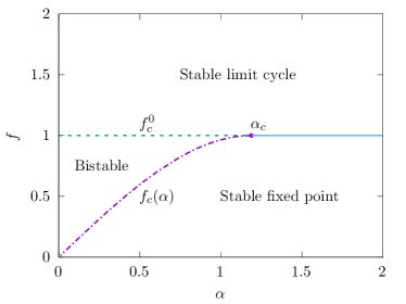
Figure 1: Phase diagram of Eq. (1) for a driven particle in the washboard potential $V(x)=-\cos(x)$, in the large-time asymptotics. Control parameters are the driving force $f>0$ and the damping parameter $\alpha\equiv\gamma/\sqrt{m}$. In the stable limit cycle domain, the mean velocity $v$ of the particle is finite (and the motion is periodic), while it is zero in the stable fixed point domain (the particle is pinned in a local minimum). In the bistable regime, whether $v=0$ of $v>0$ depends on the initial conditions. The magenta dash-dotted line $f_{c}(\alpha)$ represents a homoclinic bifurcation, the green dashed line a finite-period saddle-node bifurcation, while the solid light blue line is an infinite period bifurcation. The lines are obtained using standard numerical integration methods for Eq. (1). In this paper we obtain analytical expressions for $f_{c}(\alpha)$ in the $\alpha\to 0$ limit for an arbitrary pinning potential $V(x)$, and we describe the universal power-law behavior of $f_{c}(\alpha)$ in the $\alpha\to\alpha_{c}$ limit when approaching the triple point where the three bifurcation lines meet.

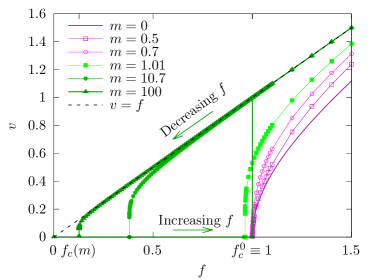
Figure 2: Hysteresis loops in the velocity-force characteristics for $V(x)=-\cos(x)$ in Eq. (1). For high damping, corresponding to masses $m<m_{c}$ at fixed $\gamma$, with $\gamma=1$ in this case, the particle depins at $f_{c}^{0}\equiv 1$ (magenta lines with empty points), without displaying hysteresis. For masses $m>m_{c}$ (green lines with filled points), there is a hysteretic depinning: Slowly increasing the applied force from $f=0$, the particle depins at $f_{c}^{0}$, acquiring a finite steady-state velocity only above it. Then, slowly decreasing $f$ from above $f_{c}^{0}$, the particle gets pinned only at the critical force $f_{c}(m)<f_{c}^{0}$. In this paper we analytically calculate the hysteretic range $[f_{c}^{0}-f_{c}(m)]$ for masses close to $m_{c}$.

Compared to the overdamped case, far fewer analytical results are known for the inertial dynamics [$m>0$ in Eq. (1)]. Now the phase diagram depends not only on the properties of the tilted potential $V(x)-fx$ but also on the relative values of the mass $m$ and the friction $\gamma$. For the paradigmatic case $V(x)=-\cos(x)$, the representative phase diagram as a function of the damping parameters $\alpha=\gamma/\sqrt{m}$ and $f$ is qualitatively well known Levi et al. (1978); Strogatz (2018), and shown in Fig. 1. It is characterized by three bifurcations lines meeting at a triple point. As in the zero-mass case, the line $f=f_{c}^{0}$ delimitates the region where the tilted potential has local minima ($f<f_{c}^{0}$) or not ($f\geq f_{c}^{0}$). For $\alpha>\alpha_{c}$, the damping is strong and having a zero velocity or not depends only on this intrinsic property of the tilted potential: The depinning transition occurs at $f_{c}^{0}$. It is described by an infinite-period bifurcation where the stable fixed point annihilates with the unstable fixed point and disappears as $f\uparrow f_{c}^{0}$. For $f>f_{c}^{0}$, the existence of a stable limit cycle implies $v>0$, and as in the overdamped case, $v\sim(f-f_{c}^{0})^{1/2}$ (though with a nontrivial $\alpha$-dependent prefactor). As $\alpha\to\infty$, one recovers the zero-mass case.

In contrast, for $\alpha<\alpha_{c}$, the damping is low enough to allow a bistable regime when $f_{c}(\alpha)<f<f_{c}^{0}$. In that regime, there is a coexistence between a stable point (a minimum of the tilted potential) for which $v=0$, and limit cycle (where inertia allows the particle to cross barriers) for which $v>0$. Initial conditions determine whether $v=0$ or $v>0$, and varying $f$ slowly leads to hysteresis (see Fig. 2). The phase-space trajectories of Fig. 3 illustrate the possible orbits in each regime. Note that the transition line $f_{c}(\alpha)$ for $\alpha<\alpha_{c}$ is described by a homoclinic bifurcation, for which the depinning transition occurs as $v\sim 1/|\log[f-f_{c}(\alpha)]|$ as $f\downarrow f_{c}(\alpha)$. Such logarithmic behavior, corresponding to a “0” depinning exponent $\beta$, is in sharp contrast with the $\beta>0$ exponent that governs the transition for $\alpha>\alpha_{c}$. Although the phase diagram of Fig. 1 is obtained for the particular case $V(x)=-\cos(x)$, it is qualitatively the same for any smooth periodic potential presenting a single minimum and maximum, as we show in this paper.

II Summary of the results

We focus on the behavior of the homoclinic bifurcation line, which separates the stable fixed point regime from the bistable one (see Fig. 2). We will use two complementary view points: either varying directly the damping constant $\alpha=\gamma/\sqrt{m}$, or, at fixed friction $\gamma$, varying the mass $m$. The critical line will respectively be denoted by $f_{c}(\alpha)$ or $f_{c}(m)$. At fixed $\gamma$, to the critical damping $\alpha_{c}$ corresponds a critical mass $m_{c}=(\gamma/\alpha_{c})^{2}$, above which inertial effects matter.

As seen on Fig. 1, on the one hand $f_{c}(\alpha)$ tends to zero when $\alpha\to 0$ (i.e., in the weakly damped limit) while it goes smoothly to $f_{c}^{0}$, as $\alpha\to\alpha_{c}$. For $V(x)=-\cos(x)$, Guckenheimer and Holmes used Melnikov’s technique Mel’nikov (1963) to show that $f_{c}(\alpha)\sim 4\alpha/\pi$ as $\alpha\to 0$ Guckenheimer and Holmes (1983). Rather surprisingly, to the best of our knowledge, no analytical prediction regarding the way $f_{c}(\alpha)$ approaches $f_{c}^{0}$ as $\alpha\to\alpha_{c}$ nor any expression for $\alpha_{c}$ were reported.

Yet, as we show, the line $f_{c}(\alpha)$ presents universal and scaling properties which are important to understand if we wish to use Eq. (1) as a toy model for more complex extended systems with inertia. These were not reported neither and in this work we provide elements to fill this gap. To do so, we employ a method to derive analytically $f_{c}^{0}-f_{c}(\alpha)$ as a function of $\alpha$ close to the triple point ($\alpha-\alpha_{c}\ll\alpha_{c}$), including explicit expressions for $\alpha_{c}$. We generalize the $\alpha\to 0$ asymptotics $f_{c}(\alpha)\sim 4\alpha/\pi$ obtained by Guckenheimer and Holmes Guckenheimer and Holmes (1983) for the cosine potential to the case of an arbitrary potential. We also show that while the $\alpha\to 0$ asymptotic scaling $f_{c}(\alpha)\propto\alpha$ is rather insensible to the details of the periodic potential, the scaling behavior when $\alpha\to\alpha_{c}$ is of the form $f_{c}^{0}-f_{c}(\alpha)\sim(\alpha_{c}-\alpha)^{\delta}$, where the exponent $\delta>0$ depends on the normal form of the bifurcation at $f_{c}^{0}$ for $\alpha>\alpha_{c}$. If, near the saddle-node bifurcation point $x^{*}$, the force can be expanded as $f-V^{\prime}(x)\approx(f-f_{c}^{0})+k|x-x^{*}|^{\Upsilon}+\ldots$, with $k$ a positive constant and $\Upsilon>1$, we obtain that $\delta=\Upsilon$. In particular, for the cosine potential $V(x)=-\cos(x)$, which corresponds to the paradigmatic pendulum and Josephson-junction problems, we obtain that the homoclinic line is characterized by the scaling $f_{c}^{0}-f_{c}(\alpha)\sim(\alpha_{c}-\alpha)^{\delta}$, with $\delta=2$.

We also show that the values of $\alpha_{c}$, $f_{c}(\alpha)$ and of the prefactor of the scaling laws are nonuniversal but depend on the details of $V(x)$ that are relevant for a precise interplay among dissipation, inertia, and drive. They can nevertheless be also estimated analytically. To obtain these results we exploit the fact that, associated to the homoclinic bifurcation at $f_{c}(\alpha)$, there exists a “critical trajectory,” or homoclinic orbit, that connects a local maximum of the tilted potential to the next one, on an infinite time window and with $\dot{x}\to 0$ at both extremal points [see Fig. 3 (b)]. This homoclinic orbit cannot be obtained analytically in general, and presents no obvious scaling form. To study it in spite of these issues, we use a tilted periodic potential $\mathcal{V}_{F}(x)$, different from the original one $V(x)-fx$, but which has the advantage that the homoclinic orbit at $f_{c}(\alpha)$ can be found exactly (it is a dissipative soliton). We then map the exact critical properties derived for the effective potential to the ones of the original tilted potential $V(x)-fx$, to estimate $f_{c}(\alpha)$ in the regimes of interest. We show that the procedure is quite general and applies to various cases.

For the standard $\Upsilon=2$ case, we find

$$f_{c}(\alpha) \sim\mathcal{N}\alpha, [\alpha\to 0]$$ (2)

$$f_{c}^{0}-f_{c}(\alpha) \sim(\alpha_{c}-\alpha)^{2}, [\alpha_{c}-\alpha\to 0^{+}]$$ (3)

$$v \sim(f-f_{c}^{0})^{1/2}, [\alpha>\alpha_{c},f-f_{c}^{0}\to 0^{+}]$$ (4)

with an exact determination of the prefactor $\mathcal{N}$ [see Eq. (59)]. In the more general case of an arbitrary value of the exponent $\Upsilon$, one finds

$$f_{c}(\alpha) \sim\mathcal{N}\alpha, \alpha\to 0$$ (5)

$$f_{c}^{0}-f_{c}(\alpha) \sim(\alpha_{c}-\alpha)^{\Upsilon}, [\alpha_{c}-\alpha\to 0^{+}]$$ (6)

$$v \sim(f-f_{c}^{0})^{1-\frac{1}{\Upsilon}}, [\alpha>\alpha_{c},f-f_{c}^{0}\to 0^{+}]$$ (7)

with the same expression for the prefactor $\mathcal{N}$.

III Organization of the paper

In Sec. IV, we review the properties of the critical trajectory which separates static from running solutions in the bistable regime. Then in Sec. V, we present a particular periodic potential, along with also a particular way of tilting it, from which $f_{c}(\alpha)$ for $\alpha<\alpha_{c}$, and $\alpha_{c}$ can be determined analytically. We show how to use the results obtained from the modified tilted potential in order to estimate these properties for the paradigmatic case $V(x)\propto-\cos(x)$. Scaling forms and characteristic quantities, are discussed. In Sec. V.7, we generalize the approach for the more general case $1<\Upsilon\neq 2$, and discuss the universality of the different results. In Section VI, we review and generalize the large-damping approach of Guckenheimer and Holmes, which allows us to determine exactly $f_{c}(\alpha)$ in the regime $\alpha\ll\alpha_{c}$ for a generic potential. Section VII presents numerical validation of our predictions together with additional observations. Section VIII contains our conclusions and perspectives.

IV The critical trajectory

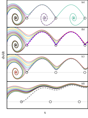
Figure 3: Phase-space trajectories obtained numerically from Eq. (1), using different initial conditions, for the weakly damped case $\alpha<\alpha_{c}$. In (a), $f<f_{c}(\alpha)$: All initial conditions starting at the left margin of the plot with different velocities are finally spirally attracted to one of the periodic images of the stable fixed points of the tilted washboard potential, such that $V^{\prime}(x)-f=0$ and $V^{\prime\prime}(x)>0$. In (b), $f=f_{c}(\alpha)$: Low initial velocity trajectories are trapped but large velocity trajectories approach the homoclinic orbit (in purple dashed line). In (c), $f_{c}(\alpha)<f<f_{c}^{0}$: Trajectories are either trapped or acquire a finite time-averaged velocity converging to the stable limit cycle. In (d), $f=f_{c}^{0}$: Stable fixed points disappear, and all trajectories are attracted to the running periodic orbit with a finite average velocity. With dashed lines we show trajectories starting with infinitesimally positive velocity at one of the unstable fixed points $x^{*}$ of the tilted potential (open circles), such that $V^{\prime}(x^{*})-f=0$ and $V^{\prime\prime}(x^{*})<0$. The homoclinic orbit corresponds exactly to the dash line in (b).

Central to our analysis is the computation of the critical trajectory $x^{\star}(t)$ that connects, for $f_{c}(\alpha)<f<f_{c}^{0}$ and $\alpha<\alpha_{c}$, a local maximum of the tilted potential $V(x)-fx$ to the following one in an infinite time window. In phase space, such trajectory, called the homoclinic orbit, acts as a separatrix: It separates two domains of the initial conditions: (i) those that lead to the limit cycle, which is characterized by a running periodic solution with $\dot{x}(t)>0$, and (ii) and those that end on a local minimum of the tilted potential, with $\dot{x}(t)\to 0$ as $t\to\infty$. In Fig. 3(c) we depict such two classes of trajectories. In contrast, for $f<f_{c}(\alpha)$ all initial conditions are trapped in stable fixed points, while for $f\geq f_{c}(\alpha)$ only running solutions are stable, as shown in Figs. 3(a) and 3(d), respectively. An accurate numerical analysis of the homoclinic orbit is specially difficult near the triple point $\alpha_{c}$ we are interested in, because the bistability range vanishes. To make progress we will hence adopt a complementary approach by tackling its properties analytically.

V A soluble tilted periodic potential

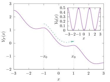
Figure 4: The nontilted (inset) and tilted (main) potentials $\mathcal{V}_{0}(x)$ and $\mathcal{V}_{F}(x)$ defined by Eqs. (8) and (9), respectively (parameters are $\mu=g=1$ and $F=\frac{1}{2}F_{c}^{0}$). A critical trajectory $x^{\star}(t)$ of a massive particle, with the dynamics (10), is represented with a green dashed line: It joins the location $-x_{0}$ of a local maximum at time $t=-\infty$ to its periodic image $x_{0}$ at time $t=\infty$.

In the definition (1) of the model, we considered a generic pinning potential $V(x)$ and we also took as an example potential a cosine function. In this section, we study a special form of potential, a periodically replicated quartic double-well potential. It allows us to obtain the exact critical trajectory and to obtain the exponents of the critical region of the homoclinic line close to the triple point.

Consider a potential

$$\mathcal{V}_{0}(x)=-\frac{g}{2}x^{4}+\mu^{2}x^{2}$$ (8)

defined on $[-x_{0},x_{0}]$ with $x_{0}=\frac{\mu}{\sqrt{g}}$. Since it is even [i.e., $\mathcal{V}_{0}(-x_{0})=\mathcal{V}_{0}(x_{0})$] we can make it periodic on $\mathbb{R}$. We also denote $\mathcal{V}_{0}(x)$ (see Fig. 4) this periodic potential.

To model the drive of a particle living in such potential out of equilibrium, we tilt the potential $\mathcal{V}_{0}(x)$ as

$$\mathcal{V}_{F}(x)=\mathcal{V}_{0}(x)-\left(x-\frac{x^{3}}{3x_{0}^{2}}\right)F,$$ (9)

where the constant $F$ represents the amplitude of a driving force. The driving force can be made periodic in the same way as for $\mathcal{V}_{0}(x)$, in the sense that the force $-\mathcal{V}^{\prime}_{F}(x)$ corresponding to $\mathcal{V}_{F}(x)$ is periodic. The resulting tilted potential $\mathcal{V}_{F}(x)$ is shown on Fig. 4. The form (9) of the drive includes a cubic contribution on top of the usual linear one, which seems unnatural but allows us to find an exact expression of the critical trajectory (the homoclinic orbit) at nonzero mass. The relation between the parameters $\{g,\mu,F\}$ of this effective model and those of a physical one will be discussed in Sec. V.3. We stress that the relation between the effective drive $F$ and the force $f$ of the original model does not take a simple form on the whole range of forces of interest. Note in passing that the form (9) of the drive ensures that the locations of the local maxima of $\mathcal{V}_{0}(x)$ are unchanged: they remain in $\pm x_{0}$ as $F$ increases.

V.1 An exact critical trajectory at nonzero mass

Let us consider the dissipative dynamics (1) of a massive particle in the potential $\mathcal{V}_{F}(x)$,

$$m\ddot{x}+\gamma\dot{x}=-\mathcal{V}^{\prime}_{F}(x)\>.$$ (10)

For values of the drive $F$ less than the critical drive

$$F^{0}_{c}=2\frac{\mu^{3}}{\sqrt{g}}\>,$$ (11)

we see that the tilted potential (9) presents local minima. This implies that at zero mass the particle gets trapped into a local minimum and the average velocity is zero. At nonzero mass, if the initial position of the particle is close enough to a local minimum, then the velocity at long times is also zero. We now determine the condition on the mass allowing, in some range $F_{c}(m)<F<F^{0}_{c}$, for the coexistence of another class of trajectories that converge to a limit cycle, and hence possesses a nonzero average velocity $v$.

We find by direct computation that, for $F<F_{c}^{0}$, there exists a critical trajectory $x^{\star}(t)$ joining two local maxima of $\mathcal{V}_{F}(x)$ located in $-x_{0}$ and $x_{0}$, between times $t=-\infty$ and $t=\infty$ (see Fig. 4). It takes the form

$$x^{\star}\!(t)=x_{0}\tanh\frac{t}{\tau}\qquad\text{with}\qquad\tau=\frac{\sqrt{M_{c}(F)}}{\mu}\>,$$ (12)

provided the mass $m$ has the value

$$M_{c}(F)=\frac{1}{4}\bigg{(}\frac{F_{c}^{0}}{F}\bigg{)}^{2}\bigg{(}\frac{\gamma}{\mu}\bigg{)}^{2}\>.$$ (13)

The existence of such explicit solution for the critical trajectory is not immediate, because in presence of dissipation ($\gamma>0$) and drive ($F>0$) the evolution equation (10) does not preserve energy anymore and there is no conserved quantity along the trajectory.

V.2 Critical mass and homoclinic bifurcation

The interpretation of the solution (12) and (13) is that of a trajectory $x^{\star}(t)$ that allows the particle to cross a barrier of potential (for $F<F_{c}^{0}$) by use of inertia, provided its mass takes the precise value $M_{c}(F)$. Such trajectory has the threshold mass that allows it to store enough kinetic energy when going downhill to precisely compensate for the friction-induced dissipation along its course. We call such a trajectory an “inertial critical trajectory.” In mathematical terms, such a trajectory is a separatrix joining the unstable point $-x_{0}$ to its periodic image $x_{0}$, allowing for a homoclinic bifurcation.

Physically, if we fix a drive $F<F_{c}^{0}$, and increase the mass $m$ starting from $m=0$ (keeping every other parameters fixed), then the mass $M_{c}(F)$ is the first mass for which a trajectory joining two local maxima of $\mathcal{V}_{F}(x)$ starts to exist. Based on this, we now determine the critical mass $m_{c}$ of the dynamics that corresponds (at fixed $\gamma$) to the critical damping $\alpha_{c}$. We prove that the critical mass is equal to:

$$m_{c}=\frac{1}{4}\bigg{(}\frac{\gamma}{\mu}\bigg{)}^{2}\>.$$ (14)

For the demonstration of this relation, we denote $m^{\star}_{c}=\frac{1}{4}\big{(}\frac{\gamma}{\mu}\big{)}^{2}$.

• Proof that $m_{c}\geq m_{c}^{\star}$: Consider a drive $F<F_{c}^{0}$. For all masses $m<m_{c}^{\star}$, we see from (13) that $m<m_{c}^{\star}<M_{c}(F)$, and hence there exists no inertial critical trajectory. We thus have proved that for all $m<m_{c}^{\star}$ the asymptotic velocity is 0. Hence, as announced, $m_{c}\geq m_{c}^{\star}$.

• Proof that $m_{c}\leq m_{c}^{\star}$: For a drive $F<F_{c}^{0}$, consider a mass $m>m_{c}^{\star}$. We see from (13) that there exists a domain of drive $[F_{c}(m),F_{c}^{0}]$ such that, $\forall F\in[F_{c}(m),F_{c}^{0}]$, there is an inertial critical trajectory. Since this is possible for all $m>m_{c}^{\star}$, this shows as announced that $m_{c}\leq m_{c}^{\star}$. Note that the exact explicit expression of $F_{c}(m)$ is

  $$F_{c}(m)=\sqrt{\frac{m_{c}}{m}}\,F_{c}^{0}\>.$$ (15)

From the previous reasoning, we see that the expression (15) is precisely that of the homoclinic bifurcation line of the model (on the range of mass $m>m_{c}$). Translating the results (14) and (15) from the variable $m$ (at fixed $\gamma$) to the damping variable $\alpha=\gamma/\sqrt{m}$, one obtains the following expressions for the critical damping $\alpha_{c}$ and the homoclinic line $F_{c}(\alpha)$:

$$\alpha_{c} =2\mu\>,$$ (16)

$$F_{c}(\alpha) =\frac{\alpha}{2\mu}=\frac{\alpha}{\alpha_{c}}\qquad\text{(for $\alpha\in[0,\alpha_{c}]$)}\>.$$ (17)

We emphasize that the relation between the effective drive $F$ and the physical force $f$ is not direct: As we now detail, these parameters are not scaling in the same way in the two regimes of interest (the low-damping limit and the vicinity of the triple point). In particular, if the homoclinic line $F_{c}(\alpha)$ is linear in $\alpha$ when $\alpha$ approaches $\alpha_{c}$ from below, then this will not be the case for $f_{c}(\alpha)$.

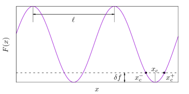
Figure 5: Landscape of force $F(x)=-V^{\prime}(x)+f$ at external force $f$ close to depinning ($f=f_{c}^{0}-\delta\!f$ with $\delta\!f>0$), presenting the critical points $x_{c}^{\pm}=x_{c}\pm\sqrt{\delta\!f/\kappa}\,$.

V.3 Parameters of the effective model close to the depinning point of a physical model

We now come back to the model of Eq. (1) with a generic periodic potential $V(x)$ of spatial period $\ell$, and we assume that it is monotonous between its unique minimum and the closest maxima (see Fig. 5). A concrete example is given by the cosine potential

$$V_{\cos}(x)=\mathfrak{f}_{0}\ell\,\frac{\cos\frac{2\pi x}{\ell}}{2\pi}\>.$$ (18)

The corresponding force $F(x)$, to which the particle is subjected, includes an external constant force $f$ with $F(x)=-V^{\prime}(x)+f$. For the cosine potential, this gives:

$$F_{\cos}(x)=\mathfrak{f}_{0}\sin\frac{2\pi x}{\ell}+f\>.$$ (19)

Along a period, the contribution $-V^{\prime}(x)$ to the force presents a minimum in $x_{c}$. The corresponding critical force (for the zero-mass depinning) is

$$f_{c}^{0}=-V^{\prime}(x_{c})\>.$$ (20)

For an external force $f<f_{c}^{0}$ close to the $m=0$ depinning force, denoting $f=f^{0}_{c}-\delta\!f$ (with $\delta\!f>0$ and $\delta\!f\ll f^{0}_{c}$), the dynamics presents two critical points $x_{c}^{\pm}$ represented on Fig. 5. Writing that, close to $x_{c}$,

$$F(x_{c}+\delta x)=-\delta\!f+\kappa\,\delta x^{2}+\ldots$$ (21)

we find

$$x_{c}^{\pm}=x_{c}\pm\sqrt{\frac{\delta\!f}{\kappa}}+\ldots$$ (22)

Note that for the cosine potential (18) one has $f^{0}_{c}=\mathfrak{f}_{0}$, $x_{c}=\frac{3}{4}\ell$, $\kappa=2\pi^{2}\mathfrak{f}_{0}/\ell^{2}$.

We are now in position to determine the values of the parameters $\{g,\mu,F\}$ of the effective potential (8) and (9) that describe the criticality of interest. We fix

$$g=4\frac{\mu^{2}}{\ell^{2}}\>,$$ (23)

ensuring that the spatial period of the potential $\mathcal{V}_{0}(x)$ is equal to $\ell$. Then, shifting $x$ so that $-\mathcal{V}^{\prime}_{F}(x^{+}_{c})=0$, we impose the following conditions:

$$-\mathcal{V}^{\prime}_{F}(x^{-}_{c})=0\qquad\text{and}\qquad-\mathcal{V}^{\prime}_{F}(x_{c})=-\delta\!f\>,$$ (24)

which ensure that force $-\mathcal{V}^{\prime}_{F}(x)$ of the effective model presents the critical properties of $F(x)$ described on Fig. 5. Solving for $\mu$ and $F$, we thus find, for small $\delta\!f$:

$$\mu =\sqrt{\frac{\kappa\ell}{8}}+\sqrt{\frac{\delta\!f}{32\ell}}\ +\ O(\delta\!f)\>,$$ (25)

$$F =\frac{\kappa\ell^{2}}{8}-\frac{3}{8}\sqrt{\kappa\,\delta\!f}\,\ell\ +\ O(\delta\!f)\>.$$ (26)

Note that, in these expressions, we should keep both contributions of order $O(\sqrt{\vphantom{|}\delta\!f})$ to describe correctly the critical scaling.

V.4 Scaling regime $m\gtrsim m_{c}$ and $f_{c}(m)\lesssim f_{c}^{0}$

We have seen in Sec. V.2 that, for masses below the critical mass $m_{c}$ given by (14), the bistable regime drive is $[F_{c}(m),F_{c}^{0}]$ with $F_{c}^{0}$ given by (11) and $F_{c}(m)$ by (15). Using the correspondence (25) and (26) between the parameters of the effective model and those of the physical model, we find that

$$F_{c}^{0}-F=\frac{1}{2}\ell\sqrt{\kappa\,\delta\!f}\ +\ O(\delta\!f)\>.$$ (27)

This relation implies an important scaling: Close to the depinning point $f_{c}^{0}$ of the physical model ($f=f_{c}^{0}-\delta\!f$), the drive $F$ of the effective model scales as $F_{c}^{0}-F\sim\sqrt{\delta\!f}$ and not as $\sim\delta\!f$, contrarily to what we could have naively expected.

Then, considering a mass $m$ slightly above the critical mass $m_{c}$,

$$m=m_{c}+\delta m\qquad\text{with}\qquad\delta m\ll m_{c}\>,$$ (28)

we see from (15) that the size of the bistable regime is determined by

$$F_{c}^{0}-F_{c}(m)=\bigg{(}1-\sqrt{\frac{m_{c}}{m_{c}+\delta m}}\bigg{)}F_{c}^{0}=\frac{1}{2}F_{c}^{0}\,\frac{\delta m}{m_{c}}+O(\delta m^{2}).$$ (29)

Thus, we see from (27) that, for the physical force $f$, the size $\delta\!f=f_{c}^{0}-f_{c}(m)$ of the bistable regime is governed by the scaling $f_{c}^{0}-f_{c}(m)\propto(m-m_{c})^{2}$; more precisely:

$$f_{c}^{0}-f_{c}(m)=\frac{\ell^{4}\kappa^{3}}{256\,\gamma^{4}}\big{(}m-m_{c}\big{)}^{2}\quad\text{for }m\to m_{c}^{+}\>.$$ (30)

For the damping coefficient, we get

$$f_{c}^{0}-f_{c}(\alpha)=\kappa^{3}\left[\frac{\ell}{64\,\mu^{3}}\right]^{2}\big{(}\alpha_{c}-\alpha\big{)}^{2}\quad\text{for }\alpha\to\alpha_{c}^{-}\>.$$ (31)

For the cosine potential (18) we have $\kappa=2\pi^{2}\mathfrak{f}_{0}/\ell^{2}$ and thus

$$f_{c}^{0}-f_{c}(m)=\frac{\pi^{6}}{32}\,\frac{\mathfrak{f}_{0}^{3}}{\ell^{2}\,\gamma^{4}}\big{(}m-m_{c}\big{)}^{2}\>,$$ (32)

where ${\pi^{6}}/{32}\approx 30.0\,$.

V.5 Effective description on the full range of forces $[0,f_{c}^{0}]$ for the tilted cosine potential

For the cosine potential (18) the zeros $x_{c}^{\pm}$ of the corresponding force (19) are given (see Fig. 5) by

$$x_{c}^{-}=\frac{\ell}{2}+\frac{\ell\arcsin\frac{f}{\mathfrak{f}_{0}}}{2\pi}\qquad\text{and}\qquad x_{c}^{+}=\ell-\frac{\ell\arcsin\frac{f}{{\mathfrak{f}_{0}}}}{2\pi}.$$ (33)

Performing the same program as previously in order to find the parameters of the effective tilted potential $\mathcal{V}_{F}$, we impose

$$\mathcal{V}^{\prime}_{F}(x^{-}_{c})=0\qquad\text{and}\qquad-\mathcal{V}^{\prime}_{F}(x_{c})=f-f^{0}_{c}\>,$$ (34)

where $f_{c}^{0}=\mathfrak{f}_{0}$. We shift the $x$ coordinate to ensure $\mathcal{V}^{\prime}_{F}(x^{+}_{c})=0$ (before the shift one has $x_{c}=\frac{3}{4}\ell$). We find

$$F =\frac{4\pi^{2}\left(\mathfrak{f}_{0}-f\right)\arcsin\frac{f}{\mathfrak{f}_{0}}}{\left[3\pi+2\arcsin\frac{f}{\mathfrak{f}_{0}}\right]\left[\arccos\frac{f}{\mathfrak{f}_{0}}\right]{}^{2}}$$ (35)

$$\mu =\frac{\pi^{3/2}}{\arccos\frac{f}{\mathfrak{f}_{0}}\sqrt{\frac{\ell}{\mathfrak{f}_{0}-f}\left(\frac{3\pi}{2}+\arcsin\frac{f}{\mathfrak{f}_{0}}\right)}}\>,$$ (36)

where $g$ is again given by (23).

From Eqs. (11), (14), and (15), we find that the corresponding equation for the pinned or bistable homoclinic critical line $f_{c}(m)$,

$$\frac{4\sqrt{\vphantom{|^{|}}\mathfrak{f}_{0}-f_{c}(m)}\arcsin\frac{f_{c}(m)}{\mathfrak{f}_{0}}}{\gamma\arccos\frac{f_{c}(m)}{\mathfrak{f}_{0}}\ \sqrt{\ell\left(2-\frac{1}{\pi}\arccos\frac{f_{c}(m)}{\mathfrak{f}_{0}}\right)}}=\frac{1}{\sqrt{m}}\>.$$ (37)

We easily check that expanding this relation for $m$ close to $m_{c}$ and $f$ close to $f_{c}^{0}=\mathfrak{f}_{0}$ (i.e., $f=\mathfrak{f}_{0}-\delta\!f$, $\delta\!f\ll\mathfrak{f}_{0}$) we recover the result (32), which describes the behavior of the homoclinic line close to the triple point.

In the other asymptotics, for small $f$ (which corresponds to large mass along the homoclinic line), we find

$$F=\frac{16}{3\pi}f\quad\text{and}\quad\mu=2\sqrt{\frac{2}{3}\frac{\mathfrak{f}_{0}}{\ell}}\qquad\text{for}\;\>f\ll\mathfrak{f}_{0}\>.$$ (38)

In this regime, the effective drive $F$ is proportional to the tilt force $f$, as physically expected. From Eq. (14), the effective critical mass in that regime is found to be

$$m_{c}=\frac{3}{32}\frac{\ell\gamma^{2}}{\mathfrak{f}_{0}}\>,$$ (39)

and we find from (15) that the critical equation for the line between the pinned and the bistable regime is

$$f_{c}(m)\sim\frac{\pi}{8}\sqrt{\frac{3\mathfrak{f}_{0}\ell}{2m}}\,\gamma\qquad\text{for}\;\>m\gg m_{c}\>.$$ (40)

We should beware that the result of Eq. (39) on the location of the triple point is only indicative since it results from a computation done in the regime of small forces along the homoclinic line (that is, far from the triple point). Translating the result (40) to the damping variable $\alpha$, one finds

$$f_{c}(\alpha)\sim\frac{\pi}{8}\sqrt{\frac{3\mathfrak{f}_{0}\ell}{2}}\,\alpha\qquad\text{for}\;\>\alpha\ll\alpha_{c}\>.$$ (41)

We recover the expected scaling $f_{c}(\alpha)\propto\alpha$ of the large-damping limit. For the parameters $\mathfrak{f}_{0}=1$ and $\ell=2\pi$ corresponding to the cosine potential of Guckenheimer and Holmes Guckenheimer and Holmes (1983), the prefactor becomes $\frac{1}{8}\sqrt{3}\pi^{3/2}\simeq 1.21$ which is not very far from the exact prefactor $4/\pi\simeq 1.27$. This result validates our approach based on an approximate “periodicized $\varphi^{4}$” potential. A derivation of the exact prefactor $4/\pi$ and of its generalization for an arbitrary potential is done in Sec. VI.

V.6 The critical mass and its asymptotic behaviors

We note that in the regime of forces $f$ close to the triple point, critical mass coming from Eqs. (14) and (25) is $\frac{1}{\pi^{2}}\frac{\ell\gamma^{2}}{\mathfrak{f}_{0}}$, while we obtained a different numerical prefactor in (39). The reason behind this mismatch is that the approach we follow consists in approximating the tilted potential $V(x)-fx$ by the effective one, $\mathcal{V}_{F}(x)$, and that the effective parameters $\mu$, $g$ and $F$ depend on $f$ in a nontrivial way, determined by the homoclinic line force $f_{c}(m)$. The first result is derived for the asymptotics $f_{c}(m)-f_{c}^{0}\ll f_{c}^{0}$ and the second one for $f_{c}(m)\ll f_{c}^{0}$. This means that our approach predicts

$$m_{c}\approx\left\{\begin{aligned} \frac{3}{32}\frac{\ell\gamma^{2}}{\mathfrak{f}_{0}}&\qquad\text{for }\quad\frac{\ell\gamma^{2}}{\mathfrak{f}_{0}}\to 0\\[5.69054pt] \frac{1}{\pi^{2}}\frac{\ell\gamma^{2}}{\mathfrak{f}_{0}}&\qquad\text{for }\quad\frac{\ell\gamma^{2}}{\mathfrak{f}_{0}}\to\infty\>,\end{aligned}\right.$$ (42)

corresponding respectively to a regime where dissipation is low (compared to the potential barriers) and a regime where dissipation is higher and close to the maximal one allowing for a limit cycle at $f<f_{c}^{0}$. We note that the numerical prefactors in both cases of (42) are rather close: This means in the intermediate regime where $\frac{\ell\gamma^{2}}{\mathfrak{f}_{0}}$ takes a finite value, the critical mass scales as in (42) with a prefactor mildly depending on $\frac{\ell\gamma^{2}}{\mathfrak{f}_{0}}$.

V.7 Mapping for general normal forms: $\Upsilon\neq 2$

Considering a tilted force that is expanded close to its critical point as $f-V^{\prime}(x)\approx(f-f_{c}^{0})+k|x-x^{*}|^{\Upsilon}$ instead of (21), one simply replaces $\sqrt{\delta\!f}$ by $\delta\!f^{1/\Upsilon}$ in Eq. (22). This implies that the same substitution has to be done in Eqs. (25) and (26). Instead of (27), one obtains now

$$F_{c}^{0}-F\sim\delta\!f^{1/\Upsilon}\quad\text{for }\delta\!f\to 0\>.$$ (43)

Then, Eqs. (30) and (31) become

$$f_{c}^{0}-f_{c}(m) \sim(m-m_{c})^{\Upsilon}\>,$$ (44)

$$f_{c}^{0}-f_{c}(\alpha) \sim(\alpha_{c}-\alpha)^{\Upsilon}\>,$$ (45)

and are valid in the vicinity of the triple point ($m\to m_{c}^{+}$, i.e., $\alpha\to\alpha_{c}^{-}$). The large damping regime, which is more universal, is described at the end of Sec. VI.2.

VI Far from the triple point: the large-damping regime

VI.1 Settings

To understand the scaling properties of the large-damping regime, we consider that the potential $V(x)$ is described by two physical parameters, its period $\ell$ and its amplitude $V_{0}$:

$$V(x)=V_{0}\,\hat{V}(x/\ell)\>,$$ (46)

where one assumes that the rescaled potential $\hat{V}(\hat{x})$ is independent of $V_{0}$ and $\ell$. At zero friction ($\gamma=0$) and zero external force ($f=0$) the equation of motion (1) for the position of the particle—whose coordinate is denoted by $x_{0}(t)$—becomes

$$m\ddot{x}_{0}=-V^{\prime}(x_{0})$$ (47)

which, on the rescaling

$$x_{0}(t)=\ell\,\hat{x}_{0}(t/\tau)\qquad\text{with }\quad\tau=\sqrt{\frac{m\ell^{2}}{V_{0}}}$$ (48)

becomes

$$\ddot{\hat{x}}_{0}=-\hat{V}^{\prime}(\hat{x}_{0})\>.$$ (49)

Since the dynamics is conservative, its description is rather explicit. Its lowest energy solution, which starts from a local maximum of $\hat{V}(\hat{x})$—located in $\hat{x}=0$, without loss of generality—with an infinitesimally small velocity at time $t=-\infty$ and arrives at the next maximum in $\hat{x}=1$ at time $t=+\infty$, is the solution of the differential equation

$$\frac{1}{2}\left[\dot{\hat{x}}_{0}\left(\hat{t}\right)\right]^{2}=\hat{V}(0)-\hat{V}\left[\hat{x}_{0}\left(\hat{t}\right)\right]\>.$$ (50)

We denote its solution by $\hat{x}_{0}^{\star}(\hat{t})$; it is independent of the physical parameters $V_{0}$ and $\ell$ and is given by

$$\text{d}\hat{t}=\frac{\text{d}\hat{x}_{0}^{\star}}{\sqrt{2\big{[}\hat{V}(0)-\hat{V}(\hat{x}_{0}^{\star})\big{]}}}\>,\quad\text{i.e.}$$ (51)

$$\hat{t}=\int_{0}^{\hat{x}_{0}^{\star}(\hat{t})}\frac{\text{d}\hat{x}_{0}}{\sqrt{2\big{[}\hat{V}(0)-\hat{V}(\hat{x}_{0})\big{]}}}\>.$$ (52)

VI.2 Perturbation at small friction and small drive

To describe the small-dissipation asymptotics of the homoclinic curve, we now drive the system by applying a small force $f$ and adding a small dissipation $\gamma$ that ensures the energy remains finite. The motion is described by Eq. (1). For a given friction $\gamma$ and a mass $m$, we are looking for the critical value of the force $f_{c}(m)$ above which a bistable regime is possible. This homoclinic line $f_{c}(m)$ is determined by the existence of a critical solution $x^{\star}(t)$ to (1) with the boundary conditions

$$x(-\infty)=x_{c} \qquad\text{;}\qquad x(\infty)=x_{c}+\ell$$ (53)

$$\dot{x}(-\infty)=0^{+} \qquad\text{;}\qquad\dot{x}(\infty)=0\,,$$ (54)

where $x_{c}$ is the location of the maximum of $V(x)-fx$ (satisfying $x_{c}\to 0$ as $f\to 0$). On the rescaling (48) one finds

$$\ddot{\hat{x}}=-\hat{V}^{\prime}(\hat{x})\underbrace{-\frac{\gamma\tau}{m}\,\dot{\hat{x}}+\hat{f}}_{\text{``small''}}\qquad\text{where}\quad\hat{f}=\frac{f}{V_{0}/\ell}\,.$$ (55)

We consider the rescaled critical solution $\hat{x}^{\star}(t)$. Multiplying (55) by $\dot{\hat{x}}^{\star}(t)$, integrating between $t=-\infty$ and $t=+\infty$ and using the boundary conditions (53) and (54), together with $[\hat{V}]_{\hat{x}_{c}}^{\hat{x}_{c}+1}=0$ (by periodicity), one finds that necessarily

$$\frac{\gamma\tau}{m}\int_{-\infty}^{\infty}\text{d}\hat{t}\;\big{(}\dot{\hat{x}}^{\star}\big{)}^{2}=\hat{f}\,.$$ (56)

This relation is true in general for the inertial critical trajectory (for any $f$ and $\gamma$ at the critical value of the mass) and expresses the fact that the energy dissipated along this trajectory matches exactly the potential loss $\hat{f}$ on one period. If one is able to determine the expression of the critical trajectory $\hat{x}^{\star}(t)$ then Eq. (56) allows one to obtain the expression of $f_{c}(m)$. However this is not possible in general. In our asymptotics of interest ($f\to 0$, $\gamma\to 0$), since both sides are small one can replace $\dot{\hat{x}}^{\star}$ by the zero-friction zero-force solution $\dot{\hat{x}}_{0}^{\star}$. This is the essence of Melnikov’s formalism Mel’nikov (1963) but written in a theoretical physicist’s manner. Then, using (51) to convert the time integral into a spatial integral together with the expression (48) of the characteristic time $\tau$, one finds

$$\frac{\gamma\ell}{\sqrt{m\,V_{0}}}\int_{0}^{1}\text{d}\hat{x}\>\sqrt{2\big{[}\hat{V}(0)-\hat{V}(\hat{x})\big{]}}=\hat{f}\,.$$ (57)

This relation gives the criterion relating $f_{c}(m)$ and in the small damping limit:

$$f_{c}(m) =\mathcal{N}\,\frac{\gamma\,\sqrt{\vphantom{|^{1}}V_{0}}}{\sqrt{m}}\qquad\text{for }\frac{\gamma}{\sqrt{m}}\to 0$$ (58)

$$\mathcal{N} =\int_{0}^{1}\text{d}\hat{x}\>\sqrt{2\big{[}\hat{V}(0)-\hat{V}(\hat{x})\big{]}}\,.$$ (59)

Here the prefactor $\mathcal{N}$ is a numerical constant. In terms of the damping coefficient, the homoclinic asymptotics writes $f_{c}(\alpha)\sim\mathcal{N}\sqrt{V_{0}}\,\alpha$ for $\alpha\to 0$. For the cosine potential, one has $\hat{V}(\hat{x})=\cos 2\pi\hat{x}$ and $\mathcal{N}=\frac{4}{\pi}$: One recovers the result of Levi et al. Levi et al. (1978) and Guckenheimer and Holmes Guckenheimer and Holmes (1983). We note that the predictions of Eqs. (58) and (59) are independent on the regularity properties of the potential, so that they should be valid even in presence of cusps. We validate this prediction numerically in Sec. VII.2.

VII Numerical Validation

VII.1 The case of the cosine potential

In this section, we will validate our analytical results by using a numerical integration of Eq. (1) with the cosine potential of Eq. (18). Without loss of generality, we choose $\gamma=1$, $\mathfrak{f}_{0}=1$ and $\ell=2\pi$, to simplify the notation.

As we showed in Fig. 2, we obtained the steady-state time-averaged velocity of the particle, as a function of the driving force, and for different mass values. This velocity seen as a function of the mass, when the driving force is equal to the critical force of the massless particle, behaves as a power law above the critical mass, which, naively, can be described as

$$v(f\equiv f_{c}^{0})\sim(m-m_{c})^{\beta\delta}.$$ (60)

This allows us to determine the critical mass with great precision. Leaving $m_{c}$, $\beta\delta$, and a prefactor as fitting parameters, we find

$$m_{c}=0.70757\pm 0.00002,$$ (61)

and $\beta\delta=0.99\pm 0.01$, as we show on Fig. 6.

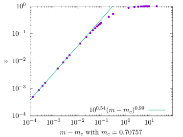
Figure 6: Steady-state time-averaged velocity as a function of the mass above the critical mass, $m-m_{c}$. With a continuous green line we show a fitted power law, where the exponent and the critical mass are fitting parameters. Then, we find $m_{c}=0.70757\pm 0.00002$.

Using the correspondence between $m$ and $\alpha=\gamma/\sqrt{m}$, we estimate from our numerical results that the critical damping is $\alpha_{c}=1.18882\pm 0.00002$, which seems to be compatible with the results from Ref. Levi et al. (1978), even if there is no explicit numerical value given by the authors. However, when comparing our estimations from Sec. V.6 with the fitted value given by Eq. (61), we only find a mild agreement. From Eq. (42), we predicted a critical mass in the range $[0.589\dots,0.637\dots]$. This mismatch comes from the fact that we are using a crude “periodicized $\varphi^{4}$ potential” approximation of the cosine potential, close to the triple point of the phase diagram. The numerical value of $m_{c}$ should depend on the exact properties of the potential on that point, thus it is not a universal property of the model and then it can only be partially estimated using that kind of approximation. The order of magnitude is correct, and, to go further, one would need to find the critical trajectory of a better approximation of the tilted potential.

Besides the critical mass, we also estimate $\beta\delta$ to be near $1$. Since $\beta=1/2$ for this model, this means $\delta=2$, which is in good agreement with the prediction from Eq. (30). Moreover, from Eq. (32) and for our choice of potential parameters, we find $f_{c}^{0}-f_{c}(m)=\frac{\pi^{4}}{128}(m-m_{c})^{2}$ close to the triple point. Comparing this to our numerical data, using the previously estimated $m_{c}$, we find an excellent agreement down to the prefactor, as can be seen in Fig. 7. This could come as a surprise, as the prediction for the critical mass was only approximate. On the one hand, the exponent $\delta$ predicted by Eq. (30) should be a universal exponent, hence more robust in the approximations made. On the other hand, the prefactor on Eq. (32) was specialized for the cosine potential, but even with the other approximations made and the fact that the prefactor should not be a universal property, the agreement is remarkably good.

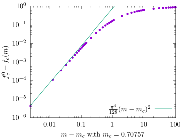
Figure 7: For the potential $V(x)=-\cos(x)$, as the mass of the particle gets close to the critical mass from above, the difference between the critical forces tends to zero as given by Eq. (32), indicated by a continuous green line. Here, we employ a numerical simulation using $\ell\equiv 2\pi$, $\gamma\equiv 1$ and $\mathfrak{f}_{0}\equiv 1$.

Last, when considering the limit $m\to\infty$, we find the known behavior from  Ref.(Guckenheimer and Holmes, 1983, Eq. (4.6.24)) which, a function of the damping parameter, as $\alpha\to 0$, is expressed as:

$$f_{c}(\alpha)=4\alpha/\pi$$ (62)

(see Sec. VI for a simple demonstration). On Fig. 8, we show that this analytical prediction is in good agreement with our numerical results.

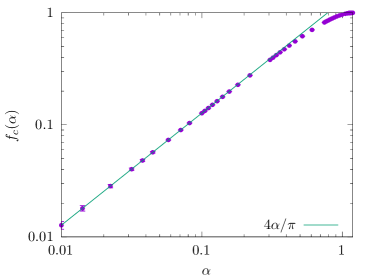
Figure 8: Critical force as a function of the damping parameter $\alpha$, defined as $\alpha=\gamma/\sqrt{m}$. The expected behavior, from Eq. (62), is correct on the limit $\alpha\ll\alpha_{c}$.

VII.2 Generic normal forms

Here, we consider the more general periodic pinning force

$$-V^{\prime}(x)=\frac{\left(\sqrt{\pi}2^{-\frac{\Upsilon}{2}}\Gamma\left(\frac{\Upsilon}{2}+1\right)\right)(1-\cos(x))^{\Upsilon/2}}{\Gamma\left(\frac{\Upsilon+1}{2}\right)}-1$$ (63)

with $\Upsilon>1$, where we have set the constant factors such that the upper critical force is $f_{c}^{0}\equiv\max_{x}[V^{\prime}(x)]=V^{\prime}(x_{c})=1$ with the marginal points fixed at $x_{c}=2\pi n$ with $n$ integer. Note that for $\Upsilon=2$, Eq. (63) reduces to the pinning force $-V^{\prime}(u)=-\cos(u)$ or simple washboard potential $V(u)=V(0)+\sin(x)$. In the $\alpha\to\infty$ overdamped limit this periodic pinning force gives rise to the normal form $\dot{x}\approx(f-f_{c}^{0})+|x-x_{c}|^{\Upsilon}$ displaying the depinning transition $v\sim(f-f_{c}^{0})^{\beta}$ with $\beta=1-1/\Upsilon$. Note that this result remains valid for $\alpha>\alpha_{c}$ finite damping and in general

$$v\sim B(\Upsilon,\alpha)(f-f_{c}^{0})^{1-1/\Upsilon}.$$ (64)

Therefore inertia does not change the critical behavior of the velocity for all the infinite-period bifurcation line $\alpha>\alpha_{c}$ although the prefactor may be affected. This result can be appreciated in Fig. 12, below the critical mass, i.e., $0\leq m\leq 0.7$.

To determine the critical mass $m_{c}$ and the behavior of $f_{c}(m)$ (particularly near the triple point $m_{c}$ and in the $m\gg m_{c}$ limit), instead of integrating Eq. (1) in time we have solved the equation

$$\frac{dK}{dx}=-\gamma\sqrt{\frac{2K}{m}}-V^{\prime}(x)+f,$$ (65)

where $K=m\dot{x}^{2}/2$ is the kinetic energy and $-V^{\prime}(x)$ is the general pinning force of Eq. (63). Equation (65), which follows directly from Eq. (1), is only valid if $\dot{x}\geq 0$ but allow us to obtain the limit-cycle trajectories directly in phase space $(x,\dot{x})$. We set $\gamma=1$ and for a given $f<f_{c}^{0}$ we prepare a limit cycle of the bistable regime, using suitable values for $m$ and initial conditions. The smallest value of the mass, $m^{*}$, that makes the limit-cycle trajectory $\dot{x}(x)$ touch the $\dot{x}=0$ axis in one point (and in all its periodic images) corresponds to the homoclinic orbit. The magenta dashed line in Fig. 3(b) illustrates one such homoclinic orbit. The pair $(f,m)\equiv(f_{c}(m),m)$ found hence belongs to the homoclinic bifurcation line. The critical mass $m_{c}$ can be determined from the vanishing of $f_{c}^{0}-f_{c}(m)$ as $m\to m_{c}$. To solve Eq. (65) numerically, for several values of $\Upsilon$ around the standard value $\Upsilon=2$, we used the Runge-Kutta Fehlberg 78 method Anhert and Mulansky (2015).

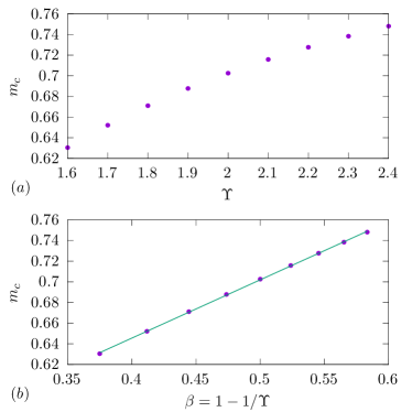
Figure 9: Critical mass $m_{c}$ vs. the normal form exponent $\Upsilon$ (a) and $\beta=1-1/\Upsilon$ (b). A fair linear fit is obtained in (b) in the full range of $\Upsilon$ shown in (a).

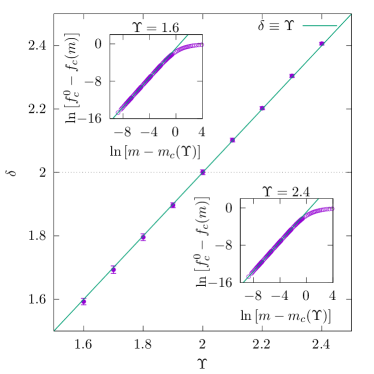
Figure 10: Critical exponent $\delta$, controlling the bistable driving force range $f_{c}^{0}-f_{c}(m)$, showing that $\delta\approx\Upsilon$ (main figure). Insets show two typical power-law fits $f_{c}^{0}-f_{c}(m)\approx\left[m-m_{c}(\Upsilon)\right]^{\delta}$ used to extract $\delta$ vs. $\Upsilon$.

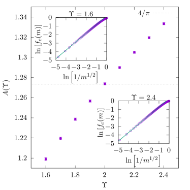
Figure 11: Large mass behavior of the critical force $f_{c}(m)$ vs. $\Upsilon$. Insets: Fits to $f_{c}(m)\approx A(\Upsilon)/\sqrt{m}$. Main figure: $A(\Upsilon)$ for a range of $\Upsilon$ around the standard $\Upsilon=2$ [or $-\cos(u)$ potential].

In the insets of Fig. 10, we show that $f_{c}^{0}-f_{c}(m)\sim(m-m_{c})^{\delta}$ as $m-m_{c}\to 0+$ for different values of $\Upsilon$, with both $m_{c}$ and $\delta$ functions of $\Upsilon$, as shown in Fig. 9 and Fig. 10 respectively. As we can appreciate in Fig. 10, $\delta$ is not an independent exponent, and $\delta\approx\Upsilon$, as predicted analytically. It is worth noting here that also depinning exponent $\beta$ is not an independent exponent, since $\beta=1-1/\Upsilon$. In other words, the bistable range is controlled by the normal form exponent corresponding to the infinite-period bifurcation for $m>m_{c}$. Summarizing,

$$f_{c}^{0}-f_{c}(m) \sim(m-m_{c})^{\Upsilon},\;\;\;\;\;\,m\lesssim m_{c}$$ (66)

$$v \sim(f-f_{c}^{0})^{1-1/\Upsilon},\;m>m_{c},\;f>f_{c}^{0}.$$ (67)

In Fig. 9 we show that $m_{c}$ is a nontrivial function of $\Upsilon$, for which we do not have analytical prediction. Interestingly, $m_{c}$ displays the behavior $m_{c}\approx a+b(1-1/\Upsilon)$ or $m_{c}(\Upsilon)\approx m_{c}(2)+b(1/2-1/\Upsilon)$ with $b$ a positive constant in the neighborhood of the standard $\Upsilon=2$ case. Finally, in Fig. 11, we show that in the homoclinic bifurcation line satisfies the following scaling form (see insets)

$$f_{c}(m)\sim A(\Upsilon)/\sqrt{m},\;\alpha\to 0$$ (68)

with $A(\Upsilon)$ a nontrivial prefactor (see main figure). One recovers as expected the Guckenheimer and Holmes prediction $A(\Upsilon=2)=4/\pi$, whose derivation is detailed in Sec. VI. The low-damping scaling $f_{c}(m)\sim 1/\sqrt{m}$ (or $f_{c}^{\alpha}\sim\alpha$) is hence robust under changes of $\Upsilon$, at variance with the $m\to m_{c}$ critical behavior which displays the $\Upsilon$-dependent exponent $\delta=\Upsilon$. All these results agree with the analytical arguments made for the more general pinning force in Sec. VI.

VIII Conclusions

We have studied the dynamical phase diagram as a function of the drive and damping of a massive particle in a periodic potential. The phase diagram consists of three different regimes, pinned, sliding and bistable, separated by three bifurcation lines, each one identified with a different type of depinning transition on driving. We have obtained analytical descriptions of the homoclinic bifurcation line which separates the bistable and the pinned regimes, both in the triple point and in the low damping limits.

The asymptotic behavior of the homoclinic bifurcation line presents interesting universal features. On one hand, for $\alpha-\alpha_{c}\to 0^{+}$, we find $f_{c}^{0}-f_{c}(\alpha)\sim(\alpha_{c}-\alpha)^{\Upsilon}$, with $\Upsilon$ representing an infinite family of periodic potentials solely characterized by the normal form describing the shape of the periodic force near its minima. The critical mass depends in a non critical way with $\Upsilon$. For the cosine potential in particular, corresponding to $\Upsilon=2$, we were able to obtain analytical estimates of the critical mass. On the the other hand, for $\alpha\to 0$, we find $f_{c}(\alpha)\sim\mathcal{N}\alpha$ and obtain an expression for $\mathcal{N}$. This scaling result was already known for $\Upsilon=2$. Nevertheless, we presented a physical argument which allows us to recover the prediction by Guckenheimer and Holmes in this particular case Guckenheimer and Holmes (1983). Interestingly, this scaling result is more robust than the triple point scaling, as it appears to be independent of the normal form exponent $\Upsilon$. To the best of our knowledge many of these properties were not reported before, particularly regarding the proximity of the triple point.

Using standard numerical methods, we have validated our analytical predictions. In the case of the cosine potential, near the triple point, the analytical result for $f_{c}^{0}-f_{c}(m)$ given by Eq. (32) is in excellent agreement with numerical data, down to the prefactor. However, the numerical result for the critical mass is close but it does not match the analytical prediction—which was an approximation—given that the critical mass is not a universal property of the model. For the generic normal forms parametrized by the exponent $\Upsilon$ we have also found a good agreement on the $\Upsilon$-dependent predicted exponents. In the latter case the critical mass follow a simple but nontrivial linear relation near $\Upsilon=2$, $m_{c}\sim a+b\beta$, with $\beta=1-1/\Upsilon$ the velocity critical exponent for $m<m_{c}$. Since we do not have an analytical prediction for this behavior, it would be interesting to tackle this problem in the future.

The analytical estimates, which we reported and validated numerically, are obtained by a nonstandard approach. This consists in mapping exact static soliton solutions in a modified tilted washboard potential to the homoclinic orbit, which separates the bistable and the pinned regimes in the original dynamical model. This approach appears to be a particularly useful alternative for an accurate description of underdamped nonuniform oscillators driven near their triple point.

Regarding possible applications of our results to concrete physical systems, it would be interesting to investigate how thermal fluctuations affect the dynamics, particularly near the triple point—either for the model we considered, or for other nonlinear dynamics that present a coupling with an inertia-like degree of freedom, e.g., in simple models of spintronic devices Lecomte et al. (2009); Barnes et al. (2012). Vollmer and Risken used a functional continued fraction approach to study the small-damping limit in presence of a noise Risken and Vollmer (1979a, b); Vollmer and Risken (1980); Risken (1996) but it would be interesting to determine if it can describe the critical regime close to the triple point.

IX Appendix

IX.1 Implementation of the numerical integration

From the computational point of view, this model does not present major difficulties when studying the cosine potential. Nevertheless, since the inertial term has a second order derivative, we employ a Verlet’s integration method to solve the dynamics. We use a Leapfrog algorithm, performing the integration in two steps: First, we calculate the velocity $v(t)$, as $v(t)\equiv\dot{x}$, and then the resulting position, at each time step. That means, at each time step $dt$ we update the velocity of the particle, as

$$v(t+dt)=v(t)+\left[{F_{\cos}(x,t)-v(t)}\right]\,\frac{dt}{m},$$ (69)

with $F_{\cos}(x,t)$ as defined on Eq. (19). Then we update the position by using the updated velocity,

$$x(t+dt)=x(t)+v(t+dt)\,dt.$$ (70)

To guarantee the stability of this method, we use a zero-acceleration initial condition for the particle, i.e., $\ddot{x}\equiv 0$. For the initial position and velocity, we fix

$$x(0)=0,\qquad v(0)=F_{\cos}(0,0)=f.$$ (71)

By using this initial condition, we study the dynamics of a particle under a range of driving forces and different values for its mass.

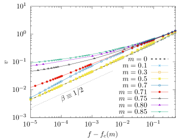
Figure 12: On the cosine potential, the steady-state time-averaged velocity, as a function of the force, undergoes different depinning transitions depending on the mass of the particle. For zero-mass, the black dashed line shows the analytical result, with $\beta=1/2$. For masses above $m_{c}$, we can only see a mild tendency toward the regime $\beta\to 0$ that describes the expected behavior $v\sim\left\{\ln[f-f_{c}(m)]\right\}^{-1}$.

Close to the depinning point, we expect different behaviors, depending on the mass of the particle. On the one hand, below the critical mass, the depinning exponent is $\beta=1/2$. On the other hand, above the critical mass, the steady-state time-averaged velocity undergoes an abrupt transition, proportional to $\left\{\ln[f-f_{c}(m)]\right\}^{-1}$ (Strogatz, 2018, Sec. 8.5). Hence, we expect $\beta\to 0$ in this case. However, the finite precision of a computer makes it very tedious to obtain such a inverse-logarithmic behavior. In Fig. 12, we illustrate how the depinning transition close to the critical mass is manifested in practice, on the velocity-force characteristics. As the mass increases, above the critical one, we observe a tendency of the critical velocity characteristics toward a regime where $\beta\to 0$ (i.e., toward a horizontal line) but studying regimes with much smaller values of $f-f_{c}(m)$ would be required in order to observe numerically the inverse-logarithmic behavior.

IX.2 Numerical method to find the critical mass

From the steady-state time-averaged velocity as a function of the mass, for a particle driven by $f=f_{c}^{0}$, we can fit the critical mass and a critical exponent using Eq. (60). Since one of the fitting parameters, $m_{c}$, is part of the argument of the power law, the fitting method is not straightforward. In our case, we fitted the data proposing different values of $m_{c}$, using only the exponent as fitting parameter. Besides the estimation for the latter, for each $m_{c}$ we test the quality of the fit using the reduced chi-square. Then, to estimate the critical mass, we simply choose the best fit, as we show in Fig. 13.

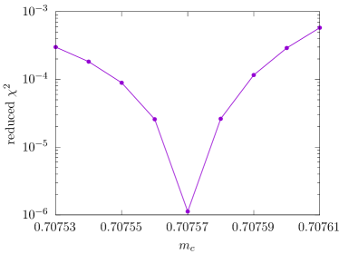
Figure 13: Using Eq. (60), we fit the exponent by proposing different values for the critical mass. Here we show the resulting reduced chi-square for each value, as a test for the goodness of fit. From the lowest value of the reduced reduced chi-square, we estimate $m_{c}=0.70757\pm 0.00002$.

References

- Strogatz (2018) S. H. Strogatz, Nonlinear Dynamics and Chaos: With Applications to Physics, Biology, Chemistry, and Engineering, 2nd ed. (CRC Press, 2018).
- Tinkham (2004) M. Tinkham, Introduction to Superconductivity, 2nd ed. (Dover Publications, 2004).
- Barone and Paternò (2005) A. Barone and G. Paternò, “Voltage current characteristics,” in Physics and Applications of the Josephson Effect (John Wiley & Sons, Ltd, 2005) Chap. 6, pp. 121–160, 1st ed.
- Purrello et al. (2017) V. H. Purrello, J. L. Iguain, A. B. Kolton, and E. A. Jagla, Phys. Rev. E 96, 022112 (2017).
- Stratonovich (1965) R. L. Stratonovich, in Non-Linear Transformations of Stochastic Processes (Elsevier, 1965) pp. 269–282.
- Ambegaokar and Halperin (1969) V. Ambegaokar and B. I. Halperin, Phys. Rev. Lett. 22, 1364 (1969).
- Doussal and Vinokur (1995) P. L. Doussal and V. M. Vinokur, Physica C: Superconductivity 254, 63 (1995).
- Scheidl (1995) S. Scheidl, Z. Physik B - Condensed Matter 97, 345 (1995).
- Risken (1996) H. Risken, The Fokker-Planck Equation: Methods of Solution and Applications, 2nd ed., Springer Series in Synergetics, Vol. 18 (Springer-Verlag Berlin Heidelberg, 1996).
- Bishop and Trullinger (1978) A. R. Bishop and S. E. Trullinger, Phys. Rev. B 17, 2175 (1978).
- Levi et al. (1978) M. Levi, F. C. Hoppensteadt, and W. Miranker, Quarterly of Applied Mathematics 36, 167 (1978).
- Mel’nikov (1963) V. K. Mel’nikov, Trudy Moskovskogo Matematicheskogo Obshchestva 12, 3 (1963).
- Guckenheimer and Holmes (1983) J. Guckenheimer and P. Holmes, Nonlinear oscillations, dynamical systems, and bifurcations of vector fields, 1st ed., Applied Mathematical Sciences, Vol. 42 (Springer-Verlag New York, 1983).
- Anhert and Mulansky (2015) K. Anhert and M. Mulansky, “Boost C++ Libraries/odeint,” https://www.boost.org/doc/libs/1_73_0/libs/numeric/odeint (2015), last revised: April 22, 2020.
- Lecomte et al. (2009) V. Lecomte, S. E. Barnes, J.-P. Eckmann, and T. Giamarchi, Phys. Rev. B 80, 054413 (2009).
- Barnes et al. (2012) S. E. Barnes, J.-P. Eckmann, T. Giamarchi, and V. Lecomte, Nonlinearity 25, 1427 (2012).
- Risken and Vollmer (1979a) H. Risken and H. D. Vollmer, Z Physik B 33, 297 (1979a).
- Risken and Vollmer (1979b) H. Risken and H. D. Vollmer, Physics Letters A 69, 387 (1979b).
- Vollmer and Risken (1980) H. D. Vollmer and H. Risken, Z Physik B 37, 343 (1980).