SCHWINGER-DYSON TYPE EQUATIONS FOR SOME QFT MODELS

The Schwinger-Dyson equations connecting free and full Green functions and vertex parts widely were used in QED for finding full Green functions under different conditions. Undoubtedly, the same approach should leads to derivation of many useful information about other models of QFT. In this work we present some technique based on variational equations for effective action to derive many different Schwinger-Dyson type equations in QFT models such as nonlinear sigma model and scalar field theory.

Key words: QED, Schwinger-Dyson equations, non-linear sigma model, effective action, vacuum expectations, $n$-point connected Green functions.

1 Introduction

Dyson [1] and Schwinger [2] had derived a system of equations which presents some integro-differential relations between free and full Green functions including vertex parts. On the base of these equations many results were obtained for QED full propagators under different conditions. But this system of equations is not closed because for vertex parts it is impossible to find a finite system of equations. This is due to that the basic equations are functional equations, and many functional relations may be obtained for different connected Green functions. But derivation of these relations mainly is based on functional integration method and this approach connected with rather complicated consideration [7] - [23]. In this paper we present a method of derivation of the Schwinger-Dyson type equations based on simple differentiation of equation for effective action. This approach follows to [4], [5] and [6]. We will see that following this approach we can derive many relations connecting different $n$-point Green functions for any QFT model.

2 Some general relations

Let’s to introduce the generator of all Green functions:

$$Z[J]=\exp\{iW[J]\}=\int{\cal{D}}\varphi\exp\{i(S+J_{i}\varphi_{i})\}.$$

Here the $\varphi_{i}$ is any field, $J_{i}$ is its external source, $W[J]$ - is the generator of all connected Green’s functions. Hereafter we will use the so-called condensed notations, for example, $J_{i}\varphi_{i}$ means $J_{i}\varphi_{i}=\int d^{4}xJ(x)\varphi(x).$ Introducing so-called classical fields

$$\varphi_{i}=\frac{\delta W[J]}{\delta J_{i}}$$ (1)

and performing following functional Legendre transformation

$$\Gamma[\varphi]=W[J]-J_{i}\varphi_{i}$$ (2)

we obtain the effective action $\Gamma[\varphi].$ According to DeWitt [3], Ch.22, the classical $S$ and quantum $\Gamma$ actions are connected as follows

$$\frac{\delta\Gamma}{\delta\varphi_{i}}=\Lambda\frac{\delta S}{\delta\varphi_{i}},$$ (3)

where the operator $\Lambda$ is constructed from connected Green functions and functional derivatives over $\varphi_{i}$:

$$\Lambda=:\exp\left\{\frac{i}{\hbar}\sum\limits_{n=2}^{\infty}\frac{(-i\hbar)^{n}}{n!}G_{i_{1}i_{2}\cdots i_{n}}\frac{\delta^{n}}{\delta\varphi_{i_{1}}\delta\varphi_{i_{2}}\cdots\delta\varphi_{i_{n}}}\right\}:,$$ (4)

where

$$G_{ij}=\frac{\delta\varphi_{i}}{\delta J_{j}}=\frac{\delta^{2}W}{\delta J_{j}\delta J_{i}},\qquad G_{i_{1}i_{2}\cdots i_{n}}=\frac{\delta^{n}W}{\delta J_{i_{1}}\delta J_{i_{2}}\cdots\delta J_{i_{n}}}$$

are connected (two- and $n$-point) Green functions. Commas in $\Lambda$ mean that derivatives act on r.h.s. expression only, not on $G^{\prime}$s. The Eq.(3) connects $\Gamma$ and $n$-point Green functions $G_{i_{1}i_{2}\cdots i_{n}}$, both of these are unknown quantity, so we need in an additional relation for them. For this purpose we will use following relation connecting the effective action $\Gamma$ and the sources $J_{i}$ - so called quantum equations of motion (see [3]):

$$\frac{\delta\Gamma}{\delta\varphi_{i}}=-J_{i}.$$ (5)

But we can approach to the Eq.(5) from another point of view - if rewrite Eq.(3) as follows

$$-J_{i}=\Lambda\frac{\delta S}{\delta\varphi_{i}},$$ (6)

with the $\Lambda$ operator as in Eq.(4) then equations for $W[J]$ will be obtained. This formula will be the main formula for us. We may rewrite it as follows:

$$-J_{i}=\frac{\delta\Gamma}{\delta\varphi^{i}}=:\exp\{\frac{i}{\hbar}\sum_{n=2}^{\infty}\frac{(-i\hbar)^{n}}{n!}G^{i_{1}i_{2}\dots i_{n}}\frac{\delta^{n}}{\delta\varphi^{i}_{1}\delta\varphi^{i}_{2}\dots\delta\varphi^{i}_{n}}\}:\frac{\delta S}{\delta\varphi^{i}},$$

Let’s to connect three-point Green function and vertex part. For this we should to differentiate (5) with respect $J_{j}:$

$$\frac{\delta}{\delta J_{j}}\frac{\delta\Gamma}{\delta\varphi_{i}}=-\delta_{ij}.$$

Due to

$$\frac{\delta\varphi_{k}}{\delta J_{l}}=\frac{\delta}{\delta J_{l}}\frac{\delta W}{\delta J_{k}}=\frac{\delta^{2}W}{\delta J_{l}\delta J_{k}}=G_{lk}$$

we get

$$\frac{\delta^{2}W}{\delta J_{l}\delta J_{k}}\frac{\delta^{2}\Gamma}{\delta\varphi_{k}\delta\varphi_{i}}=-\delta_{il}$$

Differentiating once more over $\frac{\delta}{\delta J_{s}}$ we get:

$$\frac{\delta^{3}W}{\delta J_{s}\delta J_{l}\delta J_{n}}=\frac{\delta^{2}W}{\delta J_{l}\delta J_{k}}\frac{\delta^{2}W}{\delta J_{p}\delta J_{s}}\frac{\delta^{2}W}{\delta J_{i}\delta J_{n}}\frac{\delta^{3}\Gamma}{\delta\varphi_{p}\delta\varphi_{k}\delta\varphi_{i}}$$ (7)

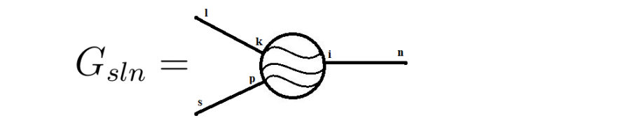
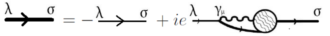
So we find a relation which connects three-point connected Green function with three-point vertex part:

$$G_{lsn}=G_{lk}G_{sp}G_{ni}\Gamma_{kpi},\qquad\Gamma_{kpi}=\frac{\delta^{3}\Gamma}{\delta\varphi_{k}\delta\varphi_{p}\delta\varphi_{i}}.$$ (8)

This is depicted in the Fig.1.

Figure 1: Three-point Green function

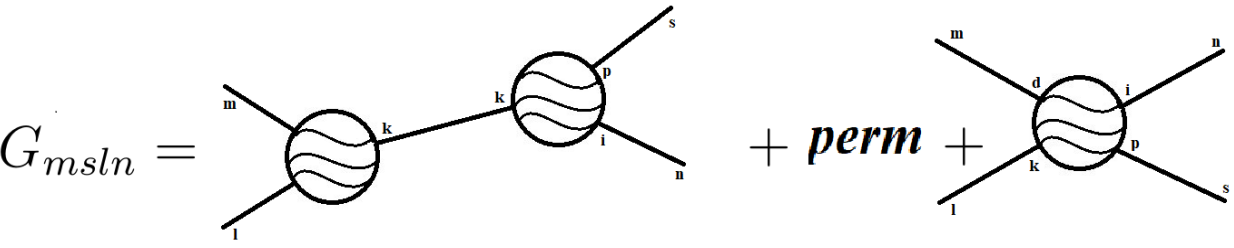
We may continue and once more differentiate Eq.(7), what gives us the following relation between four- and three- and two-point Green functions:

$$\frac{\delta^{4}W}{\delta J_{m}\delta J_{s}\delta J_{l}\delta J_{n}}=\frac{\delta^{3}W}{\delta J_{m}\delta J_{l}\delta J_{k}}\frac{\delta^{2}W}{\delta J_{p}\delta J_{s}}\frac{\delta^{2}W}{\delta J_{i}\delta J_{n}}\frac{\delta^{3}\Gamma}{\delta\varphi_{p}\delta\varphi_{k}\delta\varphi_{i}}+\\ +\frac{\delta^{2}W}{\delta J_{l}\delta J_{k}}\frac{\delta^{3}W}{\delta J_{m}\delta J_{p}\delta J_{s}}\frac{\delta^{2}W}{\delta J_{i}\delta J_{n}}\frac{\delta^{3}\Gamma}{\delta\varphi_{p}\delta\varphi_{k}\delta\varphi_{i}}+\frac{\delta^{2}W}{\delta J_{l}\delta J_{k}}\frac{\delta^{2}W}{\delta J_{p}\delta J_{s}}\frac{\delta^{2}W}{\delta J_{m}\delta J_{i}\delta J_{n}}\frac{\delta^{3}\Gamma}{\delta\varphi_{p}\delta\varphi_{k}\delta\varphi_{i}}+\\ +\frac{\delta^{2}W}{\delta J_{l}\delta J_{k}}\frac{\delta^{2}W}{\delta J_{p}\delta J_{s}}\frac{\delta^{2}W}{\delta J_{i}\delta J_{n}}\frac{\delta^{2}W}{\delta J_{m}\delta J_{d}}\frac{\delta^{4}\Gamma}{\delta\varphi_{d}\delta\varphi_{p}\delta\varphi_{k}\delta\varphi_{i}}$$

or,

$$\begin{array}[]{l}\displaystyle{G_{msln}=G_{mlk}G_{ps}G_{in}\Gamma_{pki}+G_{lk}G_{mps}G_{in}\Gamma_{pki}+}\\ \\ \displaystyle{G_{lk}G_{ps}G_{min}\Gamma_{pki}+G_{lk}G_{ps}G_{in}G_{md}\Gamma_{dpki}}.\end{array}$$ (9)

This expression ay be depicted as in the Fig:

Figure 2: Four-, three- and two-point functions.

3 Scalar $\lambda\varphi^{4}$ theory

For example, for scalar $\lambda\varphi^{4}$ theory classical action looks like:

$$S=-\frac{1}{2}\varphi_{i}(\partial^{2}+m^{2})_{ij}\varphi_{j}-\lambda\varphi^{4}=-\frac{1}{2}\varphi_{i}K^{-1}_{ij}\varphi_{j}-\lambda\varphi_{i}^{4}.$$

Applying to this classical action Eq.(6) with $\Lambda$ from (4) one can obtains equation for $W:$

$$\frac{\lambda}{6}\hbar^{2}\frac{\delta^{3}W}{\delta J_{i}^{3}}+\frac{i\lambda\hbar}{2}\frac{\delta^{2}W}{\delta J_{i}^{2}}\frac{\delta W}{\delta J_{i}}-\frac{\lambda}{6}\left(\frac{\delta W}{\delta J_{i}}\right)^{3}-K^{-1}_{ij}\frac{\delta W}{\delta J_{j}}+J_{i}=0.$$ (10)

where

$$K^{-1}_{ij}=-i\left(\partial^{2}+m^{2}\right)^{-1}\delta_{ij}$$

is free Green function. Differentiating Eq.(10) over $\dfrac{\delta}{\delta J_{k}}$ we get:

$$\frac{\hbar^{2}\lambda}{6}\frac{\delta^{4}W}{\delta J_{k}\delta J_{i}\delta J_{i}\delta J_{i}}-\frac{i\hbar\lambda}{2}\left(\frac{\delta^{3}W}{\delta J_{k}\delta J_{i}\delta J_{i}}\varphi_{i}+\frac{\delta^{2}W}{\delta J_{i}\delta J_{i}}\frac{\delta^{2}W}{\delta J_{k}\delta J_{i}}\right)-\\ -\frac{\lambda}{2}\varphi^{2}_{i}\frac{\delta^{2}W}{\delta J_{k}\delta J_{i}}-K^{-1}_{ij}\frac{\delta^{2}W}{\delta J_{k}\delta J_{j}}=-\delta_{ki}.$$

Multiplying this equation by $K_{\sigma i}$ we may obtain:

$$K_{\sigma i}\frac{\hbar^{2}\lambda}{6}\frac{\delta^{4}W}{\delta J_{k}\delta J_{i}\delta J_{i}\delta J_{i}}-K_{\sigma i}\frac{i\hbar\lambda}{2}\left(\frac{\delta^{3}W}{\delta J_{k}\delta J_{i}\delta J_{i}}\varphi_{i}+\frac{\delta^{2}W}{\delta J_{i}\delta J_{i}}\frac{\delta^{2}W}{\delta J_{k}\delta J_{i}}\right)-\\ -K_{\sigma i}\frac{\lambda}{2}\varphi^{2}_{i}\frac{\delta^{2}W}{\delta J_{k}\delta J_{i}}-K_{\sigma i}K^{-1}_{ij}\frac{\delta^{2}W}{\delta J_{k}\delta J_{j}}=-K_{\sigma i}\delta_{ki}$$

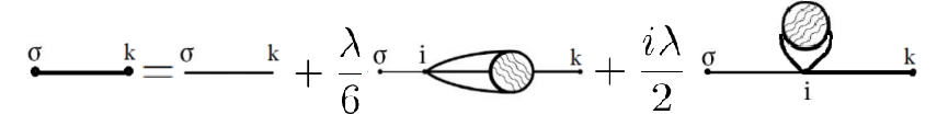
Putting $(J=0)$ we find equation for full Green function - the Schwinger-Dyson equation:

$$G^{\sigma k}=K_{\sigma k}+\frac{\hbar^{2}\lambda}{6}K_{\sigma i}G^{kiii}+\frac{i\hbar\lambda}{2}K_{\sigma i}(G^{kii}\varphi_{i}+G^{ii}G_{ki})-\frac{\lambda}{2}\varphi^{2}_{i}G^{ki}K_{\sigma i}$$ (11)

This equation is presented in the Fig.3.

Figure 3: Graphical representation of the Schwinger-Dyson equation for $\lambda\varphi^{4}/4$ theory

4 The case of QED

In [4] the following set of equations for QED effective action was derived:

$$-J_{\mu}=e\bar{\Psi}\gamma^{\mu}\Psi+D^{-1\mu\nu}A_{\nu}+ie\hbar\mathrm{Tr}\left(\gamma^{\mu}\frac{\delta^{2}W}{\delta\eta\delta\bar{\eta}}\right).$$ (12)

$$-\eta_{\alpha}=((-\hat{\partial}-m+e\hat{A})\Psi)^{\alpha}-ie\hbar(\gamma_{\mu})^{\alpha\beta}\frac{\delta^{2}W}{\delta J_{\mu}\delta\bar{\eta}^{\beta}}.$$ (13)

$$\bar{\eta}_{\alpha}=\left(\bar{\Psi}\left(i\overleftarrow{\hat{\partial}}-e\hat{A}+m\right)\right)^{\alpha}-ie\hbar\left(\gamma_{\mu}\right)^{\beta\alpha}\frac{\delta^{2}W}{\delta J_{\mu}\delta\eta^{\beta}}.$$ (14)

Here $J_{m}u,\,\eta_{i}$ and $\bar{\eta}_{i}$ are classical sources of the fields $A_{\mu},\bar{\psi}_{i}$ and $\psi_{i}$, consequently, and

$$D_{\lambda\mu}=\frac{1}{\partial^{2}}\left(g_{\lambda\mu}-(1-\alpha)\frac{\partial_{\lambda}\partial_{\mu}}{\partial^{2}}\right)$$

is free propagator of the electromagnetic field. Differentiating Eq.(12) over $\dfrac{\delta}{\delta J_{\sigma}}$ and multiplying the result by $D_{\lambda\mu}$ gives us:

$$-D_{\lambda\mu}\delta_{\sigma\mu}=eD^{\lambda\mu}\frac{\delta\bar{\Psi}}{\delta J_{\sigma}}\gamma^{\mu}\Psi+eD_{\lambda\mu}\bar{\Psi}\gamma^{\mu}\frac{\delta\Psi}{\delta J_{\sigma}}+D_{\lambda\mu}D^{-1\mu\nu}\frac{\delta^{2}W}{\delta J_{\sigma}\delta J_{\nu}}+\\ +ie\hbar D_{\lambda\mu}Tr\left(\gamma^{\mu}\frac{\delta^{3}W}{\delta J_{\sigma}\delta\eta\delta\bar{\eta}}\right).$$

In the source-free case ( $J_{\mu}=0;\eta=0;\bar{\eta}=0$ ) we get

$$G_{\lambda\sigma}=-D_{\lambda\sigma}-ie\hbar D_{\lambda\mu}Tr\left(\gamma^{\mu}\frac{\delta^{3}W}{\delta J_{\sigma}\delta\eta\delta\bar{\eta}}\right).$$

Here according to Eq.(8) we should write down:

$$\frac{\delta^{3}W}{\delta J_{\sigma}\delta\eta_{\alpha}\delta\bar{\eta}_{\beta}}=G_{\sigma\nu}G^{\alpha\rho}G^{\beta\\ tau}\frac{\delta^{3}\Gamma}{\delta A_{\nu}\delta\psi^{\rho}\delta\bar{\psi}^{\tau}}.$$

Here $G_{\sigma\nu}$ is full Green function of the photon, $G^{\alpha\beta}$ - are full Green functions of the electron. The last term is three-point vertex part. This expression is standard Schwinger-Dyson equation for QED. If the vertex part may be presented in the form

$$G^{\nu}_{\rho\tau}=\frac{\delta^{3}\Gamma}{\delta A_{\nu}\delta\psi^{\rho}\delta\bar{\psi}^{\tau}}$$

then the Schwinger-Dyson equation may be presented as follows:

$$G_{\lambda\sigma}=-D_{\lambda\sigma}-ie\hbar D_{\lambda\mu}Tr\left(\gamma^{\mu}G^{\sigma}\right).$$ (15)

Figure 4: Schwinger-Dyson equation for QED

In principle, this relation allows to calculate the full Green function of photon if we know all other terms. Let’s pass on to equation for full Green function of the electron.

$$-\eta_{\alpha}=((-\hat{\partial}-m+e\hat{A})\Psi)^{\alpha}-ie\hbar(\gamma_{\mu})^{\alpha\beta}\frac{\delta^{2}W}{\delta J_{\mu}\delta\bar{\eta}^{\beta}}$$ (16)

Differentiating this equation by $\dfrac{\delta}{\delta\eta_{\sigma}}$ we get:

$$-\delta_{\alpha\sigma}=(i\hat{\partial}-m)^{\alpha\beta}\frac{\delta\Psi_{\beta}}{\delta\eta_{\sigma}}+e\frac{\delta\left((\hat{A})^{\alpha\beta}\Psi_{\beta}\right)}{\delta\eta_{\sigma}}-ie\hbar(\gamma_{\mu})^{\alpha\beta}\frac{\delta^{3}W}{\delta\eta_{\sigma}\delta J_{\mu}\delta\bar{\eta}^{\beta}}$$

or, after somemanipulation we have standard Schwinger-Dyson equation:

$$G^{\lambda\sigma}=-S_{\lambda\sigma}+ie\hbar S_{\lambda\alpha}(\gamma_{\mu})^{\alpha\beta}G^{\mu}_{\beta\sigma}.$$ (17)

This relation is depicted in Fig.5.

Figure 5: Eq.(13)-standard Schwinger-Dyson equation for full electron Green function

5 Nonlinear $\sigma$-model

Let’s consider following model

$$\mathcal{L}=\frac{1}{2}(\partial_{\mu}\boldsymbol{\sigma})^{2}$$

where a $N$-component scalar field $\{\sigma_{a}(x),\,\,a=1,2,...,N\}$ is subject to the constraint

$$\boldsymbol{\sigma}^{2}(x)=\sum\limits_{a=1}^{N}\sigma_{a}(x)\sigma_{a}(x)=\frac{N}{\gamma}.$$ (18)

Although at first sight in the model there is no interaction but solving the constraint Eq.(18) with respect to one of the components we arrive at non-trivial interaction between remaining components. The coefficient $\gamma$ turns out to be a coupling constant. We can take into account this nontrivial structure of the model by introduction of an auxiliary field - a Lagrange multiplier - $\alpha(x)$ by the following way:

$${\cal{L}}=\frac{1}{2}(\partial_{\mu}\boldsymbol{\sigma})^{2}-\frac{1}{2}\alpha\left(\boldsymbol{\sigma}^{2}-\frac{N}{\gamma}\right),\qquad\boldsymbol{\sigma}=\{\sigma^{a},\,a=1,2,3,\,...,\,N\},$$ (19)

where $\alpha(x)$ - is an auxiliary scalar field. In the condensed notations we have for the action:

$$S=-\frac{1}{2}\sigma^{a}_{i}(\partial^{2}_{i}+\alpha_{i})\sigma^{a}_{i}+\frac{N}{2\gamma}\alpha_{i}=-\frac{1}{2}\sigma^{a}_{i}D_{ij}\sigma^{a}_{j}+\frac{N}{2\gamma}\alpha_{i},$$

where $D_{ij}=\left(\partial^{2}_{i}+\alpha_{i}\right)\delta_{ij}$. As it was shown in [5] the equations for effective action for this model has following form:

$$i\hbar\frac{\delta^{2}W}{\delta j^{i}_{a}\delta\eta_{i}}=\partial^{2}\frac{\delta W}{\delta j^{i}_{a}}+\frac{\delta W}{\eta_{i}}\frac{\delta W}{\delta j^{i}_{a}}-j^{i}_{a}$$ (20)

$$i\hbar\frac{\delta^{2}W}{\delta j^{i}_{a}\delta j^{i}_{a}}=\left(\frac{\delta W}{\delta j^{i}_{a}}\right)^{2}-\frac{N}{\gamma}-2\eta_{i}$$ (21)

Further we will work with these equations. Let’s to differentiate Eq.(20) over $j^{b}_{j}$, and Eq.(21)-over $\eta_{j}$:

$$i\frac{\delta^{3}W}{\delta j^{b}_{j}\delta j^{i}_{a}\delta\eta_{i}}=\partial^{2}\frac{\delta^{2}W}{\delta j^{b}_{j}\delta j^{i}_{a}}+\frac{\delta^{2}W}{\delta j^{b}_{j}\delta\eta_{i}}\frac{\delta W}{\delta j^{i}_{a}}+\frac{\delta W}{\delta\eta_{i}}\frac{\delta^{2}W}{\delta j^{b}_{j}\delta j^{i}_{a}}-\delta^{bi}_{ja}$$ (22)

$$i\frac{\delta^{3}W}{\delta\eta_{j}\delta j^{i}_{a}\delta j^{i}_{a}}=2\frac{\delta W}{\delta j^{i}_{a}}\frac{\delta^{2}W}{\delta\eta_{j}\delta j^{i}_{a}}-2\delta_{ji}$$ (23)

Denoting

$$G^{ib}_{aj}=\frac{\delta^{2}W}{\delta j^{i}_{a}\delta j^{b}_{j}},\qquad G^{a}_{ij}=\frac{\delta^{2}W}{\delta j^{a}_{i}\delta\eta_{j}}$$

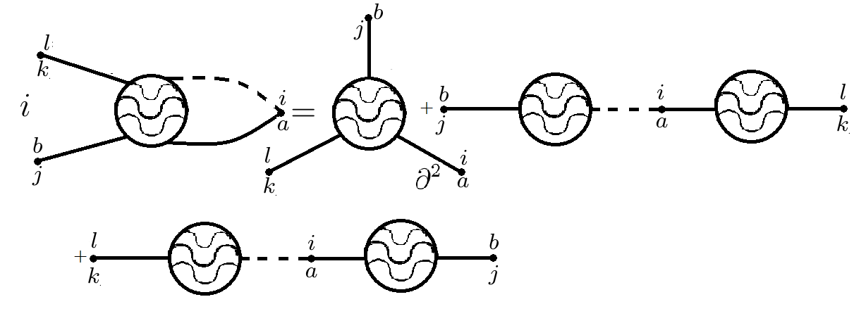
and differentiating Eq.(20)over $j^{b}_{j}$, and Eq. (21)- over $\eta_{j}$ we get the following relations for full connected Green functions:

$$\begin{array}[]{l}iG^{bi*}_{jai}=\partial^{2}G^{bi}_{ja}+G^{b*}_{ji}\sigma^{i}_{a}+\alpha_{i}G^{bi}_{ja}-\delta^{bi}_{ja};\\ iG^{*ii}_{jaa}=2\sigma^{i}_{a}G^{*i}_{ja}-2\delta_{ji}.\end{array}$$ (24)

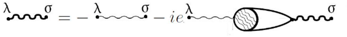
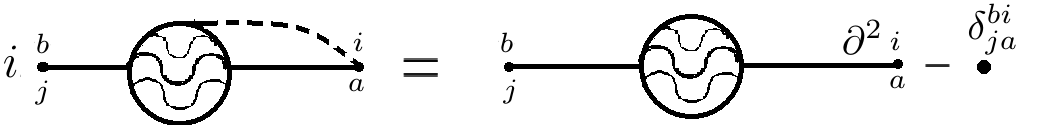
In the source-free case and supposing $\dfrac{\delta W}{\delta j^{i}_{a}}=0;\dfrac{\delta W}{\eta_{i}}=0$ we obtain the first Schwinger-Dyson type equation:

$$iG^{bi*}_{jai}=\partial^{2}G^{bi}_{ja}-\delta^{ij}\delta_{ab}.$$ (25)

This relation may be depicted as in the Fig.6.

Figure 6: Feynman diagram for Eq.25

From the second of Eq.(24) we may obtain (in the source free case)

$$G^{*ii}_{jaa}=2i\delta_{ji}.$$ (26)

Figure 7: Graphic representation for Eq.26)

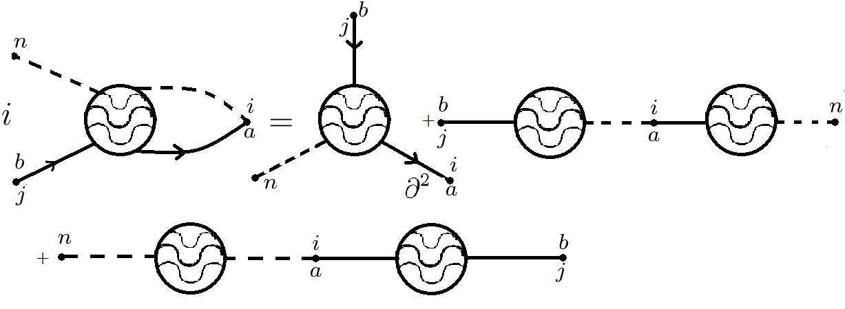
After differentiating of Eq.(21) over $j^{b}_{j}$ we get

$$i\frac{\delta^{3}W}{\delta j^{b}_{j}\delta j^{i}_{a}\delta j^{i}_{a}}=2\frac{\delta W}{\delta j^{i}_{a}}\frac{\delta^{2}W}{\delta j^{b}_{j}\delta j^{i}_{a}},$$ (27)

what may be presented as follows:

$$G^{bii}_{jaa}=2\sigma^{i}_{a}G^{bi}_{ja}.$$

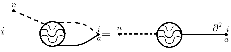
If we put sources equal to zero and suppose $\sigma_{i}^{a}=0$ in this case then

$$G^{bii}_{jaa}=0.$$ (28)

This is presented in the Fig.8.

Figure 8: Graphical representation of the Eq.(28).

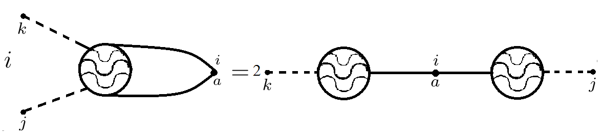
Differentiating of the Eq.(20) over $\eta_{n}$ gives us:

$$i\frac{\delta^{3}W}{\delta\eta_{n}\delta j^{i}_{a}\delta\eta_{i}}=\partial^{2}\frac{\delta^{2}W}{\delta\eta_{n}\delta j^{i}_{a}}+\frac{\delta^{2}W}{\delta\eta_{n}\delta\eta_{i}}\frac{\delta W}{\delta j^{i}_{a}}+\frac{\delta W}{\delta\eta_{i}}\frac{\delta^{2}W}{\delta\eta_{n}\delta j^{i}_{a}}.$$

Passing to Green functions we may present this as follows:

$$iG^{*i*}_{nai}=\partial^{2}G^{*i}_{na}+G^{**}_{ni}\sigma^{i}_{a}+\alpha_{i}G^{*i}_{na}.$$

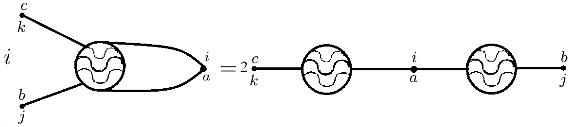
Again turning to the source-free case we have:

$$iG^{*i*}_{nai}=\partial^{2}G^{*i}_{na}.$$ (29)

what is presented in Fig.9.

Figure 9: Eq.(29) in diagrammatic form.

Let’s to differentiate Eq.(27) over $j^{c}_{k}$:

$$i\frac{\delta^{4}W}{\delta j^{c}_{k}\delta j^{b}_{j}\delta j^{i}_{a}\delta j^{i}_{a}}=2\frac{\delta^{2}W}{\delta j^{c}_{k}\delta j^{i}_{a}}\frac{\delta^{2}W}{\delta j^{b}_{j}\delta j^{i}_{a}}+2\frac{\delta W}{\delta j^{i}_{a}}\frac{\delta^{3}W}{\delta j^{c}_{k}\delta j^{b}_{j}\delta j^{i}_{a}},$$

or, through Green functions in the presence of sources:

$$iG^{cbii}_{kjaa}=2G^{ci}_{ka}G^{bi}_{ja}+2\sigma^{i}_{a}G^{cbi}_{kja}$$

In the source-free case:

$$iG^{cbii}_{kjaa}=2G^{ci}_{ka}G^{bi}_{ja},$$ (30)

which is presented in the Fig.10.

Figure 10: Eq.(30) in diagrammatic form

Taking derivative on $j^{l}_{k}$ from Eq. (22) gives us

$$i\frac{\delta^{4}W}{\delta j^{l}_{k}\delta j^{b}_{j}\delta j^{i}_{a}\delta\eta_{i}}=\partial^{2}\frac{\delta^{3}W}{\delta j^{l}_{k}\delta j^{b}_{j}\delta j^{i}_{a}}+\frac{\delta^{3}W}{\delta j^{l}_{k}\eta_{i}\delta j^{b}_{j}}\frac{\delta W}{\delta j^{i}_{a}}+\frac{\delta^{2}W}{\delta j^{b}_{j}\delta\eta_{i}}\frac{\delta^{2}W}{\delta j^{l}_{k}\delta j^{i}_{a}}+\\ +\frac{\delta^{2}W}{\delta j^{l}_{k}\delta\eta_{i}}\frac{\delta^{2}W}{\delta j^{b}_{j}\delta j^{i}_{a}}+\frac{\delta W}{\delta\eta_{i}}\frac{\delta^{3}W}{\delta j^{l}_{k}\delta j^{b}_{j}\delta j^{i}_{a}},$$

or,

$$iG^{lbi*}_{kjai}=\partial^{2}G^{lbi}_{kja}+G^{l*b}_{kij}\sigma^{i}_{a}+G^{b*}_{ji}G^{li}_{ka}+G^{l*}_{ki}G^{bi}_{ja}+\alpha_{i}G^{lbi}_{kja}.$$

$$iG^{lbi*}_{kjai}=\partial^{2}G^{lbi}_{kja}+G^{b*}_{ji}G^{li}_{ka}+G^{l*}_{ki}G^{bi}_{ja}$$ (31)

This is presented in Fig.11.

Figure 11: Eq.(31) in graphic form

Now we will take derivative of Eq.(22) over $\eta_{n}$, this gives us

$$\begin{array}[]{l}\displaystyle{i\frac{\delta^{4}W}{\delta\eta_{n}\delta j^{b}_{j}\delta j^{i}_{a}\delta\eta_{i}}=\partial^{2}\frac{\delta^{3}W}{\delta\eta_{n}\delta j^{b}_{j}\delta j^{i}_{a}}+\frac{\delta^{3}W}{\delta\eta_{n}\delta j^{b}_{j}\delta\eta_{i}}\frac{\delta W}{\delta j^{i}_{a}}}+\\ \\ \displaystyle{+\frac{\delta^{2}W}{\delta j^{b}_{j}\delta\eta_{i}}\frac{\delta^{2}W}{\delta\eta_{n}\delta j^{i}_{a}}+\frac{\delta^{2}W}{\delta\eta_{n}\delta\eta_{i}}\frac{\delta^{2}W}{\delta j^{b}_{j}\delta j^{i}_{a}}+\frac{\delta W}{\delta\eta_{i}}\frac{\delta^{3}W}{\delta\eta_{n}\delta j^{b}_{j}\delta j^{i}_{a}}},\end{array}$$ (32)

or,

$$iG^{*bi*}_{njai}=\partial^{2}G^{*bi}_{nja}+G^{*b*}_{nji}\sigma^{i}_{a}+G^{b*}_{ji}G^{*i}_{na}+G^{**}_{ni}G^{bi}_{ja}+\alpha_{i}G^{*bi}_{nja}.$$ (33)

In source-free case:

$$iG^{*bi*}_{njai}=\partial^{2}G^{*bi}_{nja}+G^{b*}_{ji}G^{*i}_{na}+G^{**}_{ni}G^{bi}_{ja}.$$ (34)

This relation is presented in Fig.12.

Figure 12: Eq.(34)

Once more differentiating Eq.(23) over $\eta_{k}$ we get:

$$i\frac{\delta^{4}W}{\delta\eta_{k}\delta\eta_{j}\delta j^{i}_{a}\delta j^{i}_{a}}=2\frac{\delta^{2}W}{\delta\eta_{k}\delta j^{i}_{a}}\frac{\delta^{2}W}{\delta\eta_{j}\delta j^{i}_{a}}+2\frac{\delta W}{\delta j^{i}_{a}}\frac{\delta^{3}W}{\delta\eta_{k}\delta\eta_{j}\delta j^{i}_{a}}.$$

This means, that

$$iG^{**ii}_{jkaa}=2G^{*i}_{ka}G^{*i}_{ja}+2\sigma^{i}_{a}G^{**i}_{kja}.$$

In source-free case we have:

$$iG^{**ii}_{jkaa}=2G^{*i}_{ka}G^{*i}_{ja}.$$ (35)

In graphic form this is presented in Fig.13:

Figure 13: Eq.(35)

6 Conclusion

We have shown that the method of variational equations for effective action gives us a powerful tool for derivation of many relations between different Green functions of any QFT models. For this derivation it is sufficient to differentiate the main equation for effective action in any QFT model as many times as it is necessary.

References

- [1] F.Dyson, Phys.Rev., v.75, 1736 (1949).
- [2] J.Schwinger, Procl. Natl. Acad. Sci., v.37, p.452(1951).
- [3] B. S. DeWitt. ”Dynamical Theory of Groups and Fields,” Gordon and Breach, New York, 1965.
- [4] B.A.Fayzullaev and M.M.Musakhanov, Two-loop effective action for theories with fermions, Annals of Phys.(NY) 241 (1995)394.
- [5] B.A.Fayzullaev, Effective action and vacuum expectations for nonlinear -model, arXiv:1510.07367.
- [6] B.A.Fazullaev, Int.Journ.of Modern Physics, Conference Series, v.49 (2019)1960006.
- [7] Fischer C.S. Infrared properties of QCD from Dyson-Schwinger equations. J.Phys. G32 (2006)253-291.
- [8] C. S. Fischer and Alkofer Phys. Rev D67 (2003) 094020, hep-ph/0301094
- [9] Maris P., Roberts C.D. Dyson-Schwinger equations: A Tool for hadronic physics. Int.J.Mod.Phys. E12 (2003)297-365.
- [10] Roberts C.D., Schmidt S.M. Dyson-Schwinger equations: Density, temperature and continuum strong QCD. Prog.Part.Nucl.Phys., 45 (2000) 1-103.
- [11] Roberts C.D., Williams A. Dyson-Schwinger equations and their application to hadronic physics. Prog.Part.Nucl.Phys., 33 (1994) 477-575.
- [12] Huber M.Q. Derivation of Dyson-Schwinger equations. physik.uni-graz.at/ mgh/notes/DerivationDSEs.pdf.
- [13] Roberts D.C. Strong QCD and Dyson-Schwinger Equations, arXiv:1203.5341v1 [nucl-th]
- [14] Foissy L. General Dyson-Schwinger equations and systems, arXiv:1112.2606v1 [math.RA]
- [15] Huber M.Q., Mitter M. CrasyDSE: A framework for solving Dyson-Schwinger equations. Comput. Phys. Commun. 2012 Nov;183(11):2441-2457.
- [16] Yeats Karen, Rearranging Dyson-Schwinger Equations, Memoirs of the American Mathematical Society 2011; 82 pp;
- [17] Campagnari D., Reinhardt H. Variational and Dyson-Schwinger equations of Hamiltonian quantum chromodynamics Phys. Rev. D 97(2018), 054027.
- [18] Wilson P., Reinhardt H. The Coulomb gauge ghost Dyson-Schwinger equation, Phys.Rev. D82:125010, arXiv:1007.2583[hep-ph](2010).
- [19] Kreimer D. A Lecture series: DYSON-SCHWINGER EQUATIONS, https://www2.mathematik.hu-berlin.de/ kreimer/wp-content/uploads/SkriptDSE.pdf
- [20] Flyvbjerg H. Dyson-Schwinger equations for the nonlinear sigma model: perturbative solution on a finite lattice., J. of Phys. A: Mathematical and General, 22(1989)3393.
- [21] Reinhard A., von Smekal L., Watson P. The Kugo-Ojima Confinement Criterion from Dyson-Schwinger Equations, Workshop on Dynamical Aspects of the QCD Phase Transition (2001 : Trento, Italy), http://arxiv.org/abs/hep-ph/0105142.
- [22] P.O. Bowman, U. M. Heller, D. B. Leinweber, M. B. Parappilly, and A. G. WilliamsPhys. Rev.D70 (2004) 034509, hep-lat/0402032.
- [23] A. Sternbeck, E. M. Ilgenfritz, M. Mueller-Preussker, and A. Schiller Phys. Rev. D72 (2005) 014507, hep-lat/0506007.