Complex Langevin: Boundary terms at poles
Abstract
We discuss the problem of possible boundary terms at poles of the drift in the complex Langevin method, which spoil correctness of the method. For the simplest, however paradigmatic cases we can find complete answers. Lessons for more generic cases as well as open mathematical problems are discussed.
I Introduction
The complex Langevin (CL) method has been studied for almost 40 years parisi ; klauder , but it still has unsolved mathematical aspects. We have given a formal justification of the method in aarts1 ; aarts2 , pointing out already the possible failure of the justification due to unwanted boundary terms “at infinity”. In an interesting paper, which among other results presents some new criteria for the possible failure of the CL method, Salcedo salc provided a different perspective on these boundary terms.
In scherzer1 and scherzer2 we studied these boundary terms in great detail for some models, leading to verifiable criteria for correctness and even to the computation of corrections in cases of failure. Since we were dealing with holomorphic drifts, all these boundary terms were at infinity, resulting from slow decay of the probability, since we were dealing with holomorphic drifts.
A particularly thorny issue is the problem of meromorphic drift arising from zeroes of the complex density defining the models, a problem that is unavoidable in finite density QCD due to zeroes of the fermion determinant. This makes it necessary to consider also boundary terms at the singularities of the drift. Nishimura and Shimasaki studied this problem for simple models nishi ; Aarts et al. pole later presented a detailed study of this issue, with the emphasis on numerical analysis of various models from the simplest one-dimensional case to full QCD.
In this paper I am beginning a mathematical analysis of the boundary terms at poles of the drift, focusing on the simplest model already studied in pole , the so-called one-pole model. In fact, I start with a further simplification of that model in which only the pole term of the drift is kept; this allows to clarify the issue by carrying out explicit calculations. A heuristic justification for this simplification is the realization that near the pole, this term dominates the drift, so neglecting the rest of the drift should be a good approximation of the CL process while it is spending time in the neighborhood of the poles. In this simple approximation the linkage of the failure of the CL method with the appearance of boundary terms at the poles becomes manifest.
In pole it was incorrectly claimed that those boundary terms had been found in the long time equilibrium limit; this error was pointed out by Salcedo salcedo ; see the erratum to pole . So here we move away from equilibrium and consider the short time evolutions, where we do find indeed the sought for boundary terms.
For the benefit of the reader we briefly recapitulate the general idea of the formal justification of the CL method and show where boundary terms may arise at poles of the drift, invalidating the formal justification.
I consider a complex density on
| (1) |
where extends to an entire analytic function, but with possible zeroes (in which case is of course multivalued).
The complex Langevin equation (CLE) in the form used here is
| (2) |
where is the Wiener process normalized as
| (3) |
and the drift is given by
| (4) | |||
| (5) |
The drift thus is univalued but has simple poles at the zeroes of . The average of a generic holomorphic observable is denoted by
| (6) |
where is the probability density on produced by the CL process starting at and running for time ; the time evolution of is given by the Fokker-Planck equation (FPE). We say that the CL process yields correct results if agrees with the “correct” expectation value of the same observable defined as
| (7) |
i. e. if
| (8) |
In aarts1 ; aarts2 it was shown that correctness is assured if the so-called interpolating function
| (9) |
is independent of the parameter . Here is the solution of the initial value problem
| (10) |
The interpolation property follows from
| (11) |
so
| (12) |
from which correctness (8) can be deduced. The left-hand side of (12), via integration by parts, is equal to a boundary term, arising from possible slow decay at infinity as well as from poles of the drift. Details are found for instance in aarts1 ; pole .
II The need to consider the evolution before reaching equilibrium
In scherzer1 ; scherzer2 we found boundary terms at infinity by considering the equilibrium distributions. But we could not find boundary terms near poles that way, because the equilibrium distribution of the probability density was always found to vanish at least linearly at the poles of the drift, so holomorphic observables could not lead to boundary terms at the pole, as we will see.
The argument goes as follows: for simplicity let us assume that there is a pole at the origin; for the boundary term arising in equilibrium and for (see pole ) consider
| (13) |
Using integration by parts and the Cauchy-Riemann equations (13) is
| (14) |
(where is the Fokker-Planck operator, see aarts1 ), since the first term of the left-hand side vanishes in equilibrium. is a boundary term. Now, since is holomorphic, has at most a simple pole at the origin, stemming from the pole in the drift. Since vanishes linearly at the origin, the integrand of (13) is bounded in the region of integration, hence the boundary term vanishes for . If we consider the time evolution for finite time , the boundary term now is given by
| (15) |
and the first term of this expression is no longer zero. In fact, below we will give an example where the second term of (15) vanishes, but there is a boundary term arising solely from the first term of (15).
The main difficulty is now to understand the evolution (10) of observables in the presence of poles. We focus on the simplest model, dubbed one-pole model in pole . Since the equilibrium distribution does not lead to a boundary term, in this note we focus on the short time evolution, and we do indeed find boundary terms there.
III The one-pole model
The action for the one-pole model can be written (after shifting the contour of integration) as
| (16) |
| (17) |
with a positive integer. The drift of the CL process is then given by the real and imaginary parts of
| (18) |
and the complex Langevin operator determining the evolution of holomorphic observables is
| (19) |
where we wrote
| (20) |
and we later use the same symbol for the partial derivative.
IV The “pure pole model”:
Since we are not analyzing the equilibrium distribution we have the freedom to study systems that do not possess one; this leads to the consideration of the one-pole model for . This is the absolutely simplest model having a pole in the drift. Since plays no role, we also set it equal to zero.
We compare the finite time evolution of the probability density under the CL process with the evolution of the observables under (10) or equivalently the semigroup . The two evolutions should be consistent if there are no boundary terms (see aarts1 ; aarts2 ; pole ).
For the system could be treated by a real Langevin process. We will nevertheless study the system in the complex domain by choosing a complex starting point for the Langevin process.
IV.1
IV.1.1 The evolution
The Langevin operator for this special case is
| (21) |
For there is a simplification, pointed out already in pole : is related to the Langevin operator with zero drift by a similarity transformation:
| (22) |
and hence
| (23) |
with the integral kernel
| (24) |
Here is to be understood as an integration variable along the real axis. The evolution of a holomorphic observable is thus given by
| (25) |
For the observables and this yields
| (26) |
| (27) |
| (28) |
| (29) |
and
| (30) |
More generally, it is easy to prove inductively that for any is a polynomial in ; for even it is holomorphic, while for odd it is meromorphic with a simple pole at . So applied to polynomial observables is indeed given by the exponential series, which actually terminates after finitely many terms.
IV.1.2 Comparison with the FPE evolution
To study the FPE evolution, we have to resort to numerical simulation. We proceed by running 10000 trajectories of the CL process all with a fixed starting point , stopping after Langevin times .
Comparing the FPE results with those of the evolution, we find there is good agreement for the even powers but drastic disagreement for the odd ones, except for very small times.
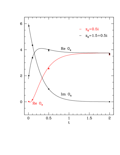
In Fig.1 we show two plots comparing the evolution of the even powers and with the corresponding results and based on the FPE, for starting points , and .
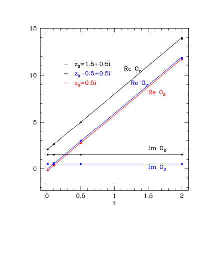
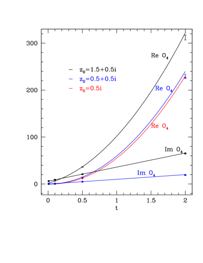
The agreement between the FPE and evolutions for even powers corresponds to the fact that in this case there are no terms appearing, hence no boundary terms at the origin.
The opposite is true for the odd powers, there is strong disagreement, indicating the presence of a boundary term. As an example we show in Fig.2 the comparison of the FPE and evolutions for the observable and the same three starting points , and ; some data of the comparison are compiled in Table 1.
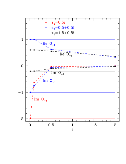
| 0.01 | 0.1 | 0.5 | 2.0 | |
| 0.45982(2)i | 0.1564(10)i | 0.05909(66)i | 0.0278(41)i | |
| 0.46I | 0.1i | -1.5i | -7.5i | |
| -0.18906(3) | 0.3435(35) | 2.727(21) | 12.0794(10) | |
| -0.19 | 0.35 | 2.75 | 11.75 | |
| -0.06623(43)i | 0.2356(34)i | 0.650(11)i | 1.284(27)i | |
| -0.0674i | 0.235i | -3.125i | -84.125i | |
| 0.01756(36) | 0.1550(46) | 12.08(20) | 226.3(3.9) | |
| 0.0185 | 0.1625 | 12.5625 | 230.063 | |
| -1.9957(21)i | -0.6297(86)i | -0.03144(58)i | -0.00356(8) i | |
| -2i | -2i | -2i | -2i |
IV.1.3 Interpolating function and boundary term
From the failure of agreement for the odd powers it is easy to see that the interpolating function is not independent of when is odd. We choose as the simplest case ; according to (30) , independent of , so according to (9)
| (31) |
From Fig.2 and Table 1 it is clear that this is not independent of , and
| (32) |
As discussed in Sec. 2, this is a boundary term, and it can only be due to the pole at , because for finite time shows strong (Gaussian) decay. It could be evaluated also directly as a boundary term, but this is not necessary.
We can also see that there is no boundary term for even observables, such as . While it is difficult to evaluate the derivative directly because it involves , we can compute the interpolating function for different values of to see that it is constant:
In Table 2 we present the values of these quantities, showing independence of within the errors.
| : |
| 2.0 | 1.99 | 1.9 | 1.5 | 0.0 | |
|---|---|---|---|---|---|
| 11.75(0) | |||||
| 230.0625(0) |
| : |
| 2.0 | 1.99 | 1.9 | 1.5 | 0.0 | |
|---|---|---|---|---|---|
| Re | 12.0(0) | ||||
| Im | 0.5(0) | ||||
| Re | 239.75(0) | ||||
| Im | 20.0(0) |
IV.2 Remarks on general
We have
| (34) |
This operator still leaves the linear space spanned by the even non-negative powers , invariant, for any integer . The odd powers for span an invariant linear space as well.
But for odd, iterating the application of to will not terminate. For even, however, it does terminate at the power ; the observable
| (35) |
is an eigenvector with eigenvalue . As for , for even and agree , whereas for the odd powers they disagree. Likewise we find that is a polynomial in ; for it will be a polynomial in , whereas for it will be a rational function of with the lowest negative power being .
As an example, we consider three observables for the case : we find by a simple calculation
| (36) |
| (37) |
| (38) |
Some data comparing with for the case are compiled in Table 3.
| 0.01 | 0.1 | 0.5 | 1.0 | 2.0 | |
| -0.14981(30) | 0.7528(50) | 4.731(30) | 9.776(61) | 19.56(12) | |
| -0.15 | 0.75 | 4.75 | 9.75 | 19.56 | |
| 0.0660(30) | 0.768(11) | 31.03(41) | 132.7(1.7) | 529.5(6.9) | |
| -0.065 | 0.7625 | 31.5625 | 133.063 | 546.063 | |
| 11.458(027 i) | 0.384(18)i | 0.384(18)i | 0.00078(7)i | 0.00013(2)i | |
| 8i | 8i | 8i | 8i | 8i |
V and
V.1
The Langevin operator is now
| (39) |
with
| (40) |
As pointed out in pole , the similarity transformation,
| (41) |
after restricting to the real axis yields in this case essentially the Hamiltonian of a harmonic oscillator
| (42) |
Equation (41) implies the relation for the semigroups
| (43) |
Note that is not positive on ; it has exactly one negative eigenmode:
| (44) |
In pole it is explained that this problem disappears if one considers on with Dirichlet boundary conditions at ; then only the odd eigenvectors contribute. Because vanishes at the (real) Langevin process avoids the origin.
In any case, because of (43) we can use Mehler’s formula barry
| (45) |
to obtain the kernel for :
| (46) |
We define
| (47) |
so that
| (48) |
Thus (46) becomes
| (49) |
with
| (50) |
We now replace by , considering it as a complex variable by analytic continuation. We consider again the observables and ; the integrals can be carried out analytically and yield
| (51) |
| (52) |
| (53) |
| (54) |
and
| (55) |
As for , the expressions for the odd powers are now meromorphic functions of , with simple poles at . For the even powers we have polynomials in .
Consistency of these results with the earlier ones for is easily verified, using
| (56) |
We can now also consider the limit , using
| (57) |
For odd grows exponentially in , whereas for even
| (58) |
and
| (59) |
which are the correct expectation values.
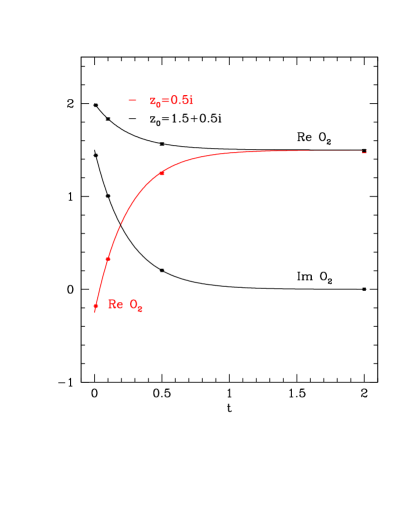
We can again compare and for finite times; qualitatively the situation is not different from the case , see Fig. 3, except that now the limit can be considered. We find again agreement for even and disagreement for odd; for the expectation values of the even powers have almost reached the infinite time limit.
As before, for odd there is strong disagreement between (which has a finite limit for ) and (which grows exponentially); this implies that the interpolating function has a nonzero slope, signaling a boundary term.
V.2 General
For this case we can still give a rather complete analysis, even though we do not have the benefit of the Mehler formula. We have
| (60) |
so the even and odd subspaces are still invariant under . For a holomorphic observable , given by a convergent power series
| (61) |
we find
| (62) |
The dual action on the coefficients is thus
| (63) |
Looking for eigenvalues of we find
| (64) |
writing
| (65) |
this can be rewritten as an upward recursion
| (66) |
There are two choices to start the recursion:
(a) at
(b) at
and the recursion will stop at . So for fixed only finitely many
will be different from in both cases.
The semigroup applied to will thus be given by a polynomial in and . We give a simple example:
| (67) |
which generalizes (52) to general . We now distinguish two cases:
-
•
even:
Let , integer. The eigenfunctions of are in case (a) even polynomials in and in case (b) odd polynomials in and , i.e. rational functions.
For the choice (a) the eigenvalues are nonpositive, corresponding to and the semigroup applied to will be given by even polynomials in .
For choice (b) there are positive and negative eigenvalues, corresponding to . The semigroup applied to will be given by odd polynomials in and , with largest negative power . In particular is an eigenfunction with the positive eigenvalue .
-
•
odd:
Let , integer.
Again for choice (a) the eigenfunctions of are even polynomials in . For (b) we obtain even polynomials in and . But the linear space of the latter contains the polynomials in arising from case (a). There is only a finite ()dimensional space of polynomials in with the highest negative power being , containing all the eigenvectors with positive eigenvalues. There are no odd eigenfunctions.
VI The general case: , ,
VI.1 Analytic considerations
This case can no longer be solved analytically, whether is real or not. It was studied numerically in pole . Here we discuss some mathematical subtleties arising in this case.
First we want to formulate a mathematical conjecture that might seem plausible, but is in general not correct:
Conjecture 1: Let be meromorphic in , holomorphic in a domain and also holomorphic in . Then there is a solution to the initial value problem (10), which is jointly holomorphic in for in any simply connected subset of and in a neighborhood of .
But conjecture 1 is wrong even for the case of being an entire function, in fact even for . The following counterexample is due to Sophie von Kowalevsky svk :
Counterexample: Let , i. e. and . Then is not analytic in at .
Proof.– is given, using the heat kernel, by
| (68) |
A closed analytic form of this could be given in terms of error functions, but it is not needed. The nonanalyticity can be seen either by looking at a power series ansatz in and for the solution, which diverges for any , or by looking at the result for , which is
| (69) |
This is clearly not analytic in at .
On the other hand we can express , using Fourier transformation, as
| (70) |
showing that for any with , is an entire function of .
Returning to our one-pole model, is still conjugate to the Hamiltonian :
| (71) |
via the similarity transformation (41). Inserting
| (72) |
the Hamiltonian becomes
| (73) |
with
| (74) |
and
| (75) |
For nonreal this is a non-Hermitian operator and we do not know much about its spectrum; in fact to give the term a precise meaning we would first have specify the space in which operates. A simple choice is .
But let us try to find the action of the semigroup on powers of . We have
| (76) |
and hence the dual action on the Taylor coefficients of is
| (77) |
The term mixes the even and odd subspaces.

Equation (77) has the structure of a downward recursion; iterating this recursion will produce nonvanishing coefficients with arbitrarily large negative. Unfortunately this will lead to coefficients growing factorially for .
Formally, will be given by a Laurent series
| (78) |
with the coefficients produced by exponentiating the recursion (77). We show in Fig. 4 the expression
| (79) |
for the observable and the parameters given in the caption. It is seen clearly that there is a linear increase, indicating that grows roughly like , so the Laurent expansion diverges for any .
We interpret this situation as follows: it is analogous to the one in the counterexample above: the semigroup applied to the powers is not analytic in at , so it cannot be constructed via the exponential series. In the counterexample there was a simple way out of this dilemma: just avoid observables with poles. Here there is also a subspace of observables that produces a convergent Laurent series (see below). But for pure powers we cannot construct the semigroup by means of the exponential series. We expect that the solutions to the initial value problem (10) exist and are meromorphic in , but in general nonanalytic in at , just as in the counterexample above.
So the analyticity properties of the solution to the initial value problem for a general holomorphic observable, where it exists, are not as simple as conjecture 1 would suggest, undermining the formal justification of the CL method.
But as stated above, it is possible to find a linear subspace of observables that do not suffer from this disease; this subspace is obtained as a deformation of the even subspace for . It can be obtained as the linear span of the eigenvectors of to nonpositive eigenvalues, which in turn are deformations of the eigenvectors obtained for =0.
The dual action (77) on the coefficients leads to the eigenvalue equation
| (80) |
This can again be rewritten as an upward recursion
| (81) |
with
| (82) |
The recursion has to start at ; the lowest coefficients are
| (83) |
For the recursion no longer terminates, but it produces a sequence decaying roughly like , thus defining an entire function of : it is not hard to prove by induction a bound of the form
| (84) |
For observables from this space we do not expect any boundary terms and the CL method should work.
We checked the correctness of the CL method numerically for the example , the eigenvector of obtained for from the upward recursion (81). We ran the recursion up to , when the coefficients are below . In Table 4 we compare the CL results with those of the evolutions. The parameters are given in the caption.
| exact | ||
|---|---|---|
| 1.14289(0) | 1.14289 | |
| 1.09798(12) | 1.09807 | |
| 0.7664(18) | 0.76610 | |
| 0.1596(79) | 0.15467 | |
| -0.015(12) | 0.02093 | |
| -0.036(12) | 0.00038 |
The table shows that the CL results are correct, possibly with a small truncation error for .
It should be noted that the recursion (81) works for any , leading to an entire function of . Of course should be excluded because it does not lead to convergence fore . But does this mean that the whole positive real axis belongs to the spectrum? This question is not well posed without specifying the space (Hilbert space, Banach space or a more general topological vector space) in which the problem is posed.
In a slightly different way, a subspace of entire functions invariant under is obtained by forming linear combinations of observables for various values of . This means that the second condition of (83) is no longer enforced, but the condition still holds. The invariance under requires that is given as
| (85) |
to preserve this relation under enforces a similar linear relation between and . Continuing this kind of reasoning, we learn that for any is a fixed multiple of with a factor that goes to zero at least linearly with . The coefficients still obey the bound (84), so this defines the subspace of entire functions invariant under ; the elements of this subspace will not give rise to boundary terms and the CL process produces correct results for them.
It would be nice to find a similar invariant subspace, consisting of functions holomorphic in , and which reduces to the odd subspace for . We could not find such a space because of the the convergence problems of the Laurent expansion discussed above. But it is clear that for observables the formal justification of the CL method fails and boundary problems are to be expected..
VI.2 Direct numerical estimation of the boundary term at
Even though we cannot solve the evolution of holomorphic observables in the general case, we can still study directly the boundary term [see (14)] at the pole numerically. Applying integration by parts in the form of Gauss’s and Green’s theorems twice to (15) one finds
| (86) |
with the outer normal to and ; see pole for details. The terms lumped together in can be seen to go to zero for in the same way we saw that in equilibrium . Omitting further contributions which are and omitting multiplicative constants, we can replace the observable by its value at the pole, replace this by and replace by
So we are reduced to considering finally
| (87) |
with . [In our reasoning we assumed . If , one has to consider higher derivatives of , which cannot all vanish, but this would lead too far afield.]
To estimate (87) numerically, we consider a sequence of rings around the pole, given by
| (88) |
with and . We chose and the starting point . The first thing to note is that the CL process needs a certain amount of time before it reaches the line . Since the motion in the direction is deterministic, we can estimate this minimal time by moving along the axis and find
| (89) |
Secondly, it is difficult to achieve sufficient statistics near the pole, because the probability density vanishes linearly at the pole, where is maximal, creating an “overlap problem”. We ran independent trajectories, but still obtained only about 50 hits for and and , and even fewer for other values of .
Therefore our results are not precise enough for a reliable extrapolation to . But we think it is fair to estimate for and .
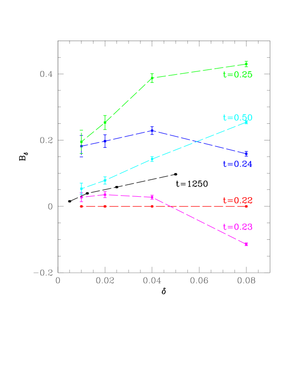
The vanishing of for explained above is confirmed by the simulation. In Fig. 5 we present the results for the Langevin times
| (90) |
and for comparison we include also equilibrium data ().
So the numerics indicate that beginning at indeed
| (91) |
decreasing again with increasing and vanishing in the long time (equilibrium) limit.
VII Conclusions and open problems
The first conclusion is that to find boundary terms at poles, it is not sufficient to look at the equilibrium distribution; it is necessary to study the short time evolution.
The second point is that quite likely the conjecture 1 (analyticity in at ) is in general not correct for the simple observables like powers of . It does seem to hold, however, for a subspace of holomorphic observables; for the one-pole model such a subspace has been constructed in Sec. VI; unfortunately for lattice models it seems very difficult imitate this construction.
Finally, for the pure pole model we established explicitly the existence of boundary terms at the pole by analyzing the short time evolution. Since in the vicinity of the pole the pole term always dominates, the pure pole model should give a good approximation of the CL process for more general models; thus we expect such boundary terms generally, provided the CL process comes arbitrarily close to the pole.
An open question concerns the analyticity properties that can be expected for the solutions of the general initial value problem (10), given the analyticity properties of the drift and the initial value . Since conjecture 1 failed, inspired by Kowalevsky’s counterexample, we formulate something weaker:
Conjecture 2. Let be meromorphic in , holomorphic in a domain and also holomorphic in . Then there is a solution to (10) which for is holomorphic in for in any simply connected subset of .
Remark. Conjcture 2 of course implies that can only have isolated singularities at the poles of ; these may be poles or essential singularities, but could also be branch points.
Conjecture 2 has implicitly been assumed to be true for instance in pole . It certainly would be worth knowing if it can be converted into a theorem.
Our experience in the previous section unfortunately suggests the following:
Conjecture 3. Let be meromorphic in , holomorphic in a domain and also holomorphic in . Then “generically” there is no solution to (10) that is holomorphic jointly in for in simply connected subsets of and in a neighborhood of .
The trouble is the lack of analyticity in at , just as found in the example above. Of course the term “generically” is a bit vague; in our model we found that for conjecture 3 holds for and , but not for and not for , .
Acknowledgments: I would like tho thank Gert Aarts, Manuel Scherzer, Dénes Sexty and Nucu Stamatescu for the long and fruitful collaboration on the CL method. Clearly this note is an outgrowth of that collaboration. I am also grateful to Denes Sexty for useful comments on this manuscript.
Appendix A Importance of using the correct function space
We want to highlight a subtlety of defining the semigroup or equivalently the initial value problem (10) by looking at a simple example. What we said about the spectrum is equally valid for the semigroup: without fixing the space in which we search for solutions, the initial value problem is not well posed.
As an example consider the observable for the pure pole model with .
The difference lies in the analyticity properties in : while for any fixed (93) is holomorphic in in the whole complex plane , it has an essential singularity in at for any fixed . Furthermore, for , the limit does not exist, so in this domain (93) does not solve the initial value problem.
Since the CL does not avoid the region , for the solution (93) the argument for correctness fails. On the other hand, the real Langevin process, occurring for real starting points, never moves into the dangerous region and reproduces the second solution for restricted to the half line .
On the other hand, as noted before, the solution (30) is meromorphic in for fixed , but holomorphic in for fixed , and solves the initial value problem correctly; here it is the pole at the origin that invalidates the formal argument by giving rise to a boundary term.
So it is essential to specify at least the analyticity domains of the solutions when attempting to construct the solution of the initial value problem (10). The real and complex cases demand different spaces.
References
- (1) G. Parisi, On complex probabilities, Phys.Lett. B131 (1983) 393–395.
- (2) J. R. Klauder, Stochastic quantization, Acta Phys.Austriaca Suppl. 25 (1983) 251–281.
- (3) G. Aarts, E. Seiler and I.-O. Stamatescu, The Complex Langevin method: When can it be trusted?, Phys.Rev. D81 (2010) 054508, [0912.3360].
- (4) G. Aarts, F. A. James, E. Seiler and I.-O. Stamatescu, Complex Langevin: Etiology and diagnostics of its main problem, Eur.Phys.J. C71 (2011) 1756, [arxiv:1101.3270].
- (5) L. L. Salcedo, Does the complex Langevin method give unbiased results?, Phys.Rev. D94 (2016) 114505 [arxiv:1611.06390].
- (6) M. Scherzer, E. Seiler, D. Sexty and I. O. Stamatescu, Complex Langevin and boundary terms, Phys.Rev. D99 (2019) 014512 [arxiv:1808.05187].
- (7) M. Scherzer, E. Seiler, D. Sexty and I.-O. Stamatescu, Controlling Complex Langevin simulations of lattice models by boundary term analysis, Phys.Rev. D101 (2020) 014501 [arxiv:1910.09427].
- (8) J. Nishimura and S. Shimasaki, New insights into the problem with a singular drift term in the complex Langevin method, Phys.Rev. D92 (2015) 011501 [arxiv:1504.08359[hep-lat]].
- (9) G. Aarts, E. Seiler, D. Sexty and I. O. Stamatescu, Complex Langevin dynamics and zeroes of the fermion determinant JHEP 1705 (2017) 044, [arxiv:1701.02322]; Erratum: JHEP 1801 (2018) 128
- (10) L. L. Salcedo, private communication.
- (11) B. Simon, Functional Integration and Quantum Physics, Academic Press, New York, 1979.
- (12) S. von Kowalevsky, Zur Theorie der partiellen Differentialgleichungen, J. für die Reine und Angew. Mathematik, 80, 1 (1975).