The Dual Information Bottleneck

Zoe Piran
Racah Institute of Physics
The Hebrew University of Jerusalem
Jerusalem, Israel
zoe.piran@mail.huji.ac.il
&Ravid Shwartz-Ziv
School of Computer Science
The Hebrew University of Jerusalem
Jerusalem, Israel
ravid.ziv@mail.huji.ac.il &Naftali Tishby
School of Computer Science
The Hebrew University of Jerusalem
Jerusalem, Israel
tishby@cs.huji.ac.il
Abstract

The Information Bottleneck (IB) framework is a general characterization of optimal representations obtained using a principled approach for balancing accuracy and complexity. Here we present a new framework, the Dual Information Bottleneck (dualIB), which resolves some of the known drawbacks of the IB. We provide a theoretical analysis of the dualIB framework; (i) solving for the structure of its solutions (ii) unraveling its superiority in optimizing the mean prediction error exponent and (iii) demonstrating its ability to preserve exponential forms of the original distribution. To approach large scale problems, we present a novel variational formulation of the dualIB for Deep Neural Networks. In experiments on several data-sets, we compare it to a variational form of the IB. This exposes superior Information Plane properties of the dualIB and its potential in improvement of the error.

1 Introduction

The Information Bottleneck (IB) method [1], is an information-theoretic framework for describing efficient representations of a β€œinput” random variable X𝑋X that preserve the information on an β€œoutput” variable Yπ‘ŒY. In this setting the joint distribution of X𝑋X and Yπ‘ŒY, p​\brkβˆ—x,y𝑝\brkπ‘₯𝑦p\brk*{x,y}, defines the problem, or rule, and the training data are a finite sample from this distribution. The stochastic nature of the label is essential for the analytic regularity of the IB problem. In the case of deterministic labels, we assume a noise model which induces a distribution. The representation variable X^^𝑋\hat{X} is in general a stochastic function of X𝑋X which forms a Markov chain Yβ†’Xβ†’X^β†’π‘Œπ‘‹β†’^𝑋Y\rightarrow X\rightarrow\hat{X}, and it depends on Yπ‘ŒY only through the input X𝑋X. We call the map p​\brkβˆ—x^∣xconditional𝑝\brk^π‘₯π‘₯p\brk*{\hat{x}\mid x} the encoder of the representation and denote by p​\brkβˆ—y∣x^conditional𝑝\brk𝑦^π‘₯p\brk*{y\mid\hat{x}} the Bayes optimal decoder for this representation; i.e., the best possible prediction of the desired label Yπ‘ŒY from the representation X^^𝑋\hat{X}.

The IB has direct successful applications for representation learning in various domains, from vision and speech processing [2], to neuroscience [3], and Natural Language Processing [4]. Due to the notorious difficulty in estimating mutual information in high dimension, variational approximations to the IB have been suggested and applied also to Deep Neural Networks (DNNs) [e.g., 5, 6, 7]. Additionally, following [8], several recent works tackled the problem of understanding DNNs using the IB principle [9, 10]

Still, there are several drawbacks to the IB framework which motivated this work. While the standard approach in representation learning is to use the topology or a specific parametric model over the input, the IB is completely non-parametric and it operates only on the probability space. In addition, the IB formulation does not relate to the task of prediction over unseen patterns and assumes full access to the joint probability of the patterns and labels.

Here, we resolve the above drawbacks by introducing a novel framework, the Dual Information Bottleneck (dualIB). The dualIB can account for known features of the data and use them to make better predictions over unseen examples, from small samples for large scale problems. Further, it emphasizes the prediction variable, Y^^π‘Œ\hat{Y}, which wasn’t present in the original IB formulation.

1.1 Contributions of this work

We present here the Dual Information Bottleneck (dualIB) aiming to obtain optimal representations, which resolves the IB drawbacks:

  • β€’

    We provide a theoretical analysis which obtains an analytical solution to the framework and compare its behaviour to the IB.

  • β€’

    For data which can be approximated by exponential families we provide closed form solutions, dualExpIB, which preserves the sufficient statistics of the original distribution.

  • β€’

    We show that by accounting for the prediction variable, the dualIB formulation optimizes a bound over the error exponent.

  • β€’

    We present a novel variational form of the dualIB for Deep Neural Networks (DNNs) allowing its application to real world problems. Using it we empirically investigate the dynamics of the dualIB and validate the theoretical analysis.

2 Background

The Information Bottleneck (IB) framework is defined as the trade off between the encoder and decoder mutual information values. It is defined by the minimization of the Lagrangian:

β„±\brk[s]βˆ—pΞ²\brkβˆ—x^∣x;pΞ²\brkβˆ—y∣x^=I(X;X^)βˆ’Ξ²I(Y;X^),\displaystyle\mathcal{F}\brk[s]*{p_{\beta}\brk*{\hat{x}\mid x};p_{\beta}\brk*{y\mid\hat{x}}}=I(X;\hat{X})-\beta I(Y;\hat{X})~{}, (1)

independently over the convex sets of the normalized distributions, \brk​[c]βˆ—pβ​\brkβˆ—x^∣xconditional\brkdelimited-[]𝑐subscript𝑝𝛽\brk^π‘₯π‘₯\brk[c]*{p_{\beta}\brk*{\hat{x}\mid x}}, \brk​[c]βˆ—pβ​\brkβˆ—x^\brkdelimited-[]𝑐subscript𝑝𝛽\brk^π‘₯\brk[c]*{p_{\beta}\brk*{\hat{x}}} and \brk​[c]βˆ—pβ​\brkβˆ—y∣x^conditional\brkdelimited-[]𝑐subscript𝑝𝛽\brk𝑦^π‘₯\brk[c]*{p_{\beta}\brk*{y\mid\hat{x}}}, given a positive Lagrange multiplier β𝛽\beta constraining the information on Yπ‘ŒY, while preserving the Markov Chain Yβ†’Xβ†’X^β†’π‘Œπ‘‹β†’^𝑋Y\rightarrow X\rightarrow\hat{X}. Three self-consistent equations for the optimal encoder-decoder pairs, known as the IB equations, define the solutions to the problem. An important characteristic of the equations is the existence of critical points along the optimal line of solutions in the information plane (presenting I​(Y;X^)πΌπ‘Œ^𝑋I(Y;\hat{X}) vs. I​(X;X^)𝐼𝑋^𝑋I(X;\hat{X})) [11, 12]. The IB optimization trade off can be considered as a generalized rate-distortion problem [13] with the distortion function, dIB​\brkβˆ—x,x^=D​\brk​[s]βˆ—p​\brkβˆ—yβ€‹βˆ£x|​|pβ​\brkβˆ—y|​x^subscript𝑑IB\brkπ‘₯^π‘₯𝐷\brkdelimited-[]𝑠𝑝\brk𝑦delimited-∣|π‘₯subscript𝑝𝛽\brk𝑦^π‘₯d_{\rm{IB}}\brk*{x,\hat{x}}=D\brk[s]*{p\brk*{y\mid x}||p_{\beta}\brk*{y|\hat{x}}}. For more background on the IB framework see Β§A.

3 The Dual Information Bottleneck

Supervised learning is generally separated into two phases: the training phase, in which the internal representations are formed from the training data, and the prediction phase, in which these representations are used to predict labels of new input patterns [14]. To explicitly address these different phases we add to the IB Markov chain another variable, Y^^π‘Œ\hat{Y}, the predicted label from the trained representation, which obtains the same values as Yπ‘ŒY but is distributed differently:

⏞training​Yβ†’Xβ†’X^Ξ²β†’Y^⏟prediction.β†’superscript⏞absenttrainingπ‘ŒsubscriptβŸβ†’π‘‹subscript^𝑋𝛽→^π‘Œprediction\displaystyle\hbox to0.0pt{$\overbrace{\phantom{Y\rightarrow X\rightarrow\hat{X}_{\beta}}}^{\textrm{training}}$\hss}Y\rightarrow\underbrace{X\rightarrow\hat{X}_{\beta}\rightarrow\hat{Y}}_{\textrm{prediction}}. (2)

The left-hand part of this chain describes the representation training, while the right-hand part is the Maximum Likelihood prediction using these representations [15]. So far the prediction variable Y^^π‘Œ\hat{Y} has not been a part of the IBIB\rm{IB} optimization problem. It has been implicitly assumed that the Bayes optimal decoder, pβ​\brkβˆ—y∣x^conditionalsubscript𝑝𝛽\brk𝑦^π‘₯p_{\beta}\brk*{y\mid\hat{x}}, which maximizes the full representation-label information, I​(Y;X^)πΌπ‘Œ^𝑋I(Y;\hat{X}), for a given β𝛽\beta, is also the best choice for making predictions. Namely, the prediction of the label, Y^^π‘Œ\hat{Y}, from the representation X^Ξ²subscript^𝑋𝛽\hat{X}_{\beta} through the right-hand Markov chain by the mixture using the internal representations, pβ​\brkβˆ—y^∣xβ‰‘βˆ‘x^pβ​\brkβˆ—y=y^β€‹βˆ£x^​pβ​\brkβˆ—x^βˆ£β€‹x,conditionalsubscript𝑝𝛽\brk^𝑦π‘₯subscript^π‘₯subscript𝑝𝛽\brk𝑦^𝑦delimited-∣∣^π‘₯subscript𝑝𝛽\brk^π‘₯π‘₯p_{\beta}\brk*{\hat{y}\mid x}\equiv\sum_{\hat{x}}p_{\beta}\brk*{y=\hat{y}\mid\hat{x}}p_{\beta}\brk*{\hat{x}\mid x}, is optimal when pβ​\brkβˆ—y∣x^conditionalsubscript𝑝𝛽\brk𝑦^π‘₯p_{\beta}\brk*{y\mid\hat{x}} is the Bayes optimal decoder. However, this is not necessarily the case, for example when we train from finite samples [16].

Focusing on the prediction problem, we define the dualIB distortion by switching the order of the arguments in the KL-divergence of the original IB distortion, namely:

ddualIB​\brkβˆ—x,x^subscript𝑑dualIB\brkπ‘₯^π‘₯\displaystyle d_{\rm{dualIB}}\brk*{x,\hat{x}} =D​\brk​[s]βˆ—pβ​\brkβˆ—yβ€‹βˆ£x^‖​p​\brkβˆ—y∣x=βˆ‘ypβ​\brkβˆ—y∣x^​log⁑pβ​\brkβˆ—y∣x^p​\brkβˆ—y∣x.absentconditional𝐷\brkdelimited-[]𝑠subscript𝑝𝛽\brk𝑦delimited-βˆ£β€–^π‘₯𝑝\brk𝑦π‘₯conditionalsubscript𝑦subscript𝑝𝛽\brk𝑦^π‘₯conditionalsubscript𝑝𝛽\brk𝑦^π‘₯conditional𝑝\brk𝑦π‘₯\displaystyle=D\brk[s]*{p_{\beta}\brk*{y\mid\hat{x}}\|p\brk*{y\mid x}}=\sum_{y}p_{\beta}\brk*{y\mid\hat{x}}\log\frac{p_{\beta}\brk*{y\mid\hat{x}}}{p\brk*{y\mid x}}\ . (3)

In geometric terms this is known as the dual distortion problem [17]. The dualIBdualIB\rm{dualIB} optimization can then be written as the following rate-distortion problem:

β„±βˆ—\brk[s]βˆ—pΞ²\brkβˆ—x^∣x;pΞ²\brkβˆ—y∣x^\displaystyle\mathcal{F}^{*}\brk[s]*{p_{\beta}\brk*{\hat{x}\mid x};p_{\beta}\brk*{y\mid\hat{x}}} =I​(X;X^)+β​𝔼pβ​\brkβˆ—x,x^​\brk​[s]βˆ—ddualIB​\brkβˆ—x,x^.absent𝐼𝑋^𝑋𝛽subscript𝔼subscript𝑝𝛽\brkπ‘₯^π‘₯\brkdelimited-[]𝑠subscript𝑑dualIB\brkπ‘₯^π‘₯\displaystyle=I(X;\hat{X})+\beta\mathbb{E}_{p_{\beta}\brk*{x,\hat{x}}}\brk[s]*{d_{\rm{dualIB}}\brk*{x,\hat{x}}}~{}. (4)

As the decoder defines the prediction stage (pβ​\brkβˆ—y=y^∣x^subscript𝑝𝛽\brk𝑦conditional^𝑦^π‘₯p_{\beta}\brk*{y=\hat{y}\mid\hat{x}}) we can write (see proof in Β§B) the average distortion in terms of mutual information on Y^^π‘Œ\hat{Y}, I​(X^;Y^)𝐼^𝑋^π‘ŒI(\hat{X};\hat{Y}) and I​(X;Y^)𝐼𝑋^π‘ŒI(X;\hat{Y}):

𝔼pβ​\brkβˆ—x,x^​\brk​[s]βˆ—ddualIB​\brkβˆ—x,x^subscript𝔼subscript𝑝𝛽\brkπ‘₯^π‘₯\brkdelimited-[]𝑠subscript𝑑dualIB\brkπ‘₯^π‘₯\displaystyle\mathbb{E}_{p_{\beta}\brk*{x,\hat{x}}}\brk[s]*{d_{\rm{dualIB}}\brk*{x,\hat{x}}} =I​(X^;Y^)βˆ’I​(X;Y^)⏟(a)+𝔼p​\brkβˆ—x​\brk​[s]βˆ—D​\brk​[s]βˆ—pβ​\brkβˆ—y^β€‹βˆ£x‖​p​\brkβˆ—y=y^∣x⏟(b).absentsubscript⏟𝐼^𝑋^π‘ŒπΌπ‘‹^π‘Œπ‘Žsubscript⏟subscript𝔼𝑝\brkπ‘₯\brkdelimited-[]𝑠𝐷\brkdelimited-[]𝑠subscript𝑝𝛽\brk^𝑦delimited-βˆ£β€–π‘₯𝑝\brk𝑦conditional^𝑦π‘₯𝑏\displaystyle=\underbrace{I(\hat{X};\hat{Y})-I(X;\hat{Y})}_{(a)}+\underbrace{\mathbb{E}_{p\brk*{x}}\brk[s]*{D\brk[s]*{p_{\beta}\brk*{\hat{y}\mid x}\|p\brk*{y=\hat{y}\mid x}}}}_{(b)}. (5)

This is similar to the known IB relation: 𝔼pβ​\brkβˆ—x,x^​\brk​[s]βˆ—dIB​\brkβˆ—x,x^=I​(Y;X)βˆ’I​(Y;X^)subscript𝔼subscript𝑝𝛽\brkπ‘₯^π‘₯\brkdelimited-[]𝑠subscript𝑑IB\brkπ‘₯^π‘₯πΌπ‘Œπ‘‹πΌπ‘Œ^𝑋\mathbb{E}_{p_{\beta}\brk*{x,\hat{x}}}\brk[s]*{d_{\rm{IB}}\brk*{x,\hat{x}}}=I(Y;X)-I(Y;\hat{X}) with an extra positive term (b)𝑏(b). Both terms, (a)π‘Ž(a) and (b)𝑏(b), vanish precisely when X^^𝑋\hat{X} is a sufficient statistic for X𝑋X with respect to Y^^π‘Œ\hat{Y}. In such a case we can reverse the order of X𝑋X and X^^𝑋\hat{X} in the Markov chain (2). This replaces the roles of Yπ‘ŒY and Y^^π‘Œ\hat{Y} as the variable for which the representations, X^Ξ²subscript^𝑋𝛽\hat{X}_{\beta}, are approximately minimally sufficient statistics. In that sense the dualIB shifts the emphasis from the training phase to the prediction phase. This implies that minimizing the dualIB functional maximizes a lower bound on the mutual information I​(X;Y^)𝐼𝑋^π‘ŒI(X;\hat{Y}).

3.1 The dualIB equations

Solving the dualIB minimization problem (4), we obtain a set of self consistent equations. Generalized Blahut-Arimoto (BA) iterations between them converges to an optimal solution. The equations are similar to the original IB equations with the following modifications: (i) Replacing the distortion by its dual in the encoder update; (ii) Updating the decoder by the encoder’s geometric mean of the data distributions p​\brkβˆ—y∣xconditional𝑝\brk𝑦π‘₯p\brk*{y\mid x}.

Theorem 1.

The dualIB equations are given by:

{\brkβˆ—ipβ​\brkβˆ—x^∣x=pβ​\brkβˆ—x^Z𝒙^βˆ£π’™β€‹\brkβˆ—x;β​eβˆ’Ξ²β€‹D​\brk​[s]βˆ—pβ​\brkβˆ—yβ€‹βˆ£x^‖​p​\brkβˆ—y∣x\brkβˆ—i​ipβ​\brkβˆ—x^=βˆ‘xpβ​\brkβˆ—x^∣x​p​\brkβˆ—x\brkβˆ—i​i​ipβ​\brkβˆ—y∣x^=1Zπ’šβˆ£π’™^​\brkβˆ—x^;Ξ²β€‹βˆxp​\brkβˆ—y∣xpβ​\brkβˆ—x∣x^,cases\brk𝑖conditionalsubscript𝑝𝛽\brk^π‘₯π‘₯subscript𝑝𝛽\brk^π‘₯subscript𝑍conditional^𝒙𝒙\brkπ‘₯𝛽superscript𝑒conditional𝛽𝐷\brkdelimited-[]𝑠subscript𝑝𝛽\brk𝑦delimited-βˆ£β€–^π‘₯𝑝\brk𝑦π‘₯\brk𝑖𝑖subscript𝑝𝛽\brk^π‘₯conditionalsubscriptπ‘₯subscript𝑝𝛽\brk^π‘₯π‘₯𝑝\brkπ‘₯\brk𝑖𝑖𝑖conditionalsubscript𝑝𝛽\brk𝑦^π‘₯conditional1subscript𝑍conditionalπ’š^𝒙\brk^π‘₯𝛽subscriptproductπ‘₯𝑝\brk𝑦superscriptπ‘₯conditionalsubscript𝑝𝛽\brkπ‘₯^π‘₯\displaystyle\begin{cases}\brk*{i}\ &p_{\beta}\brk*{\hat{x}\mid x}=\frac{p_{\beta}\brk*{\hat{x}}}{Z_{\hat{\boldsymbol{x}}\mid\boldsymbol{x}}\brk*{x;\beta}}e^{-\beta D\brk[s]*{p_{\beta}\brk*{y\mid\hat{x}}\|p\brk*{y\mid x}}}\\ \brk*{ii}\ &p_{\beta}\brk*{\hat{x}}=\sum_{x}p_{\beta}\brk*{\hat{x}\mid x}p\brk*{x}\\ \brk*{iii}\ &p_{\beta}\brk*{y\mid\hat{x}}=\frac{1}{Z_{\boldsymbol{y}\mid\hat{\boldsymbol{x}}}\brk*{\hat{x};\beta}}\prod_{x}p\brk*{y\mid x}^{p_{\beta}\brk*{x\mid\hat{x}}}\end{cases}, (6)

where Z𝐱^βˆ£π±β€‹\brkβˆ—x;Ξ²,Z𝐲∣𝐱^​\brkβˆ—x^;Ξ²subscript𝑍conditional^𝐱𝐱\brkπ‘₯𝛽subscript𝑍conditional𝐲^𝐱\brk^π‘₯𝛽Z_{\hat{\boldsymbol{x}}\mid\boldsymbol{x}}\brk*{x;\beta},Z_{\boldsymbol{y}\mid\hat{\boldsymbol{x}}}\brk*{\hat{x};\beta} are normalization terms.

The proof is given in Β§C. It is evident that the basic structure of the equations of the dualIB and IB is similar and they approach each other for large values of β𝛽\beta. In the following sections we explore the implication of the differences on the properties of the new framework.

3.2 The critical points of the dualIB

As mentioned in Β§2 and [11], the β€œskeleton” of the IB optimal bound (the information curve) is constituted by the critical points in which the topology (cardinality) of the representation changes. Using perturbation analysis over the dualIB optimal representations we find that small changes in the encoder and decoder that satisfy (6) for a given β𝛽\beta are approximately determined through a nonlinear eigenvalues problem. 111For simplicity we ignore here the possible interactions between the different representations.

Theorem 2.

The dualIB critical points are given by non-trivial solutions of the nonlinear eigenvalue problem:

\brk​[s]βˆ—Iβˆ’Ξ²β€‹Cx​xβ€²dualIB​\brkβˆ—x^,β​δ​log⁑pβ​\brkβˆ—xβ€²βˆ£x^\brkdelimited-[]𝑠𝐼𝛽subscriptsuperscript𝐢dualIBπ‘₯superscriptπ‘₯β€²\brk^π‘₯conditional𝛽𝛿subscript𝑝𝛽\brksuperscriptπ‘₯β€²^π‘₯\displaystyle\brk[s]*{I-\beta C^{\rm{dualIB}}_{xx^{\prime}}\brk*{\hat{x},\beta}}{\delta\log p_{\beta}\brk*{x^{\prime}\mid\hat{x}}} =0,\brk​[s]βˆ—Iβˆ’Ξ²β€‹Cy​yβ€²dualIB​\brkβˆ—x^,β​δ​log⁑pβ​\brkβˆ—yβ€²βˆ£x^=0.formulae-sequenceabsent0\brkdelimited-[]𝑠𝐼𝛽subscriptsuperscript𝐢dualIB𝑦superscript𝑦′\brk^π‘₯conditional𝛽𝛿subscript𝑝𝛽\brksuperscript𝑦′^π‘₯0\displaystyle=0~{},~{}~{}~{}~{}\brk[s]*{I-\beta C^{\rm{dualIB}}_{yy^{\prime}}\brk*{\hat{x},\beta}}{\delta\log p_{\beta}\brk*{y^{\prime}\mid\hat{x}}}=0. (7)

The matrices Cx​xβ€²dualIB​\brkβˆ—x^;Ξ²,Cy​yβ€²dualIB​\brkβˆ—x^;Ξ²subscriptsuperscript𝐢dualIBπ‘₯superscriptπ‘₯β€²\brk^π‘₯𝛽subscriptsuperscript𝐢dualIB𝑦superscript𝑦′\brk^π‘₯𝛽C^{\rm{dualIB}}_{xx^{\prime}}\brk*{\hat{x};\beta},C^{\rm{dualIB}}_{yy^{\prime}}\brk*{\hat{x};\beta} have the same eigenvalues \brk​[c]βˆ—Ξ»i\brkdelimited-[]𝑐subscriptπœ†π‘–\brk[c]*{\lambda_{i}}, with Ξ»1​(x^)=0subscriptπœ†1^π‘₯0\lambda_{1}(\hat{x})=0. With binary y𝑦y, the critical points are obtained at Ξ»2​\brkβˆ—x^=Ξ²βˆ’1subscriptπœ†2\brk^π‘₯superscript𝛽1\lambda_{2}\brk*{\hat{x}}=\beta^{-1}.

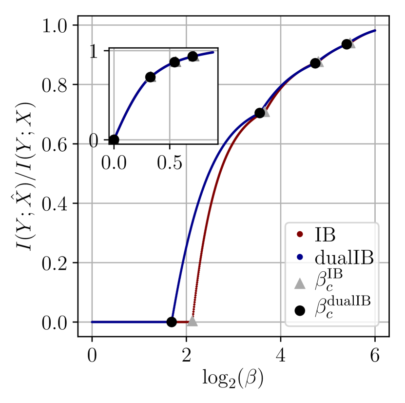
The proof to Theorem 2 along with the structure of the matrices Cx​xβ€²dualIB​\brkβˆ—x^;Ξ²,Cy​yβ€²dualIB​\brkβˆ—x^;Ξ²subscriptsuperscript𝐢dualIBπ‘₯superscriptπ‘₯β€²\brk^π‘₯𝛽subscriptsuperscript𝐢dualIB𝑦superscript𝑦′\brk^π‘₯𝛽C^{\rm{dualIB}}_{xx^{\prime}}\brk*{\hat{x};\beta},C^{\rm{dualIB}}_{yy^{\prime}}\brk*{\hat{x};\beta} is given in Β§D. We found that this solution is similar to the nonlinear eigenvalues problem for the IB, given in Β§A. As in the IB, at the critical points we observe cusps with an undefined second derivative in the mutual information values as functions of β𝛽\beta along the optimal line. That is the general structure of the solutions is preserved between the frameworks, as can be seen in FigureΒ 1(c).

The Information Plane, Iy=I​(X^;Y)subscript𝐼𝑦𝐼^π‘‹π‘ŒI_{y}=I(\hat{X};Y) vs. Ix=I​(X^;X)subscript𝐼π‘₯𝐼^𝑋𝑋I_{x}=I(\hat{X};X), is the standard depiction of the compression-prediction trade-off of the IB and has known analytic properties[18]. First, we note that both curves obey similar constraints, as given in lemmaΒ 3 below.

Lemma 3.

along the optimal lines of Ix​(Ξ²)subscript𝐼π‘₯𝛽I_{x}(\beta) and Iy​(Ξ²)subscript𝐼𝑦𝛽I_{y}(\beta) the curves are non-decreasing piece-wise concave functions of β𝛽\beta. When their second derivative (with respect to β𝛽\beta) is defined, it is strictly negative.

Next, comparing the dualIB’s and IB’s information planes we find several interesting properties which are summarized in the following Theorem (see Β§E for the proof).

Theorem 4.

(i) The critical points of the two algorithms alternate, βˆ€i,i+1for-all𝑖𝑖1\forall i,i+1, Ξ²c,idualIB≀βc,iIB≀βc,i+1dualIB≀βc,iIBsuperscriptsubscript𝛽𝑐𝑖dualIBsuperscriptsubscript𝛽𝑐𝑖IBsuperscriptsubscript𝛽𝑐𝑖1dualIBsuperscriptsubscript𝛽𝑐𝑖IB\beta_{c,i}^{\rm{dualIB}}\leq\beta_{c,i}^{\rm{IB}}\leq\beta_{c,i+1}^{\rm{dualIB}}\leq\beta_{c,i}^{\rm{IB}}. (ii) The distance between the two information curves is minimized at Ξ²cdualIBsuperscriptsubscript𝛽𝑐dualIB\beta_{c}^{\rm{dualIB}}. (iii) The two curves approach each other as Ξ²β†’βˆžβ†’π›½\beta\rightarrow\infty.

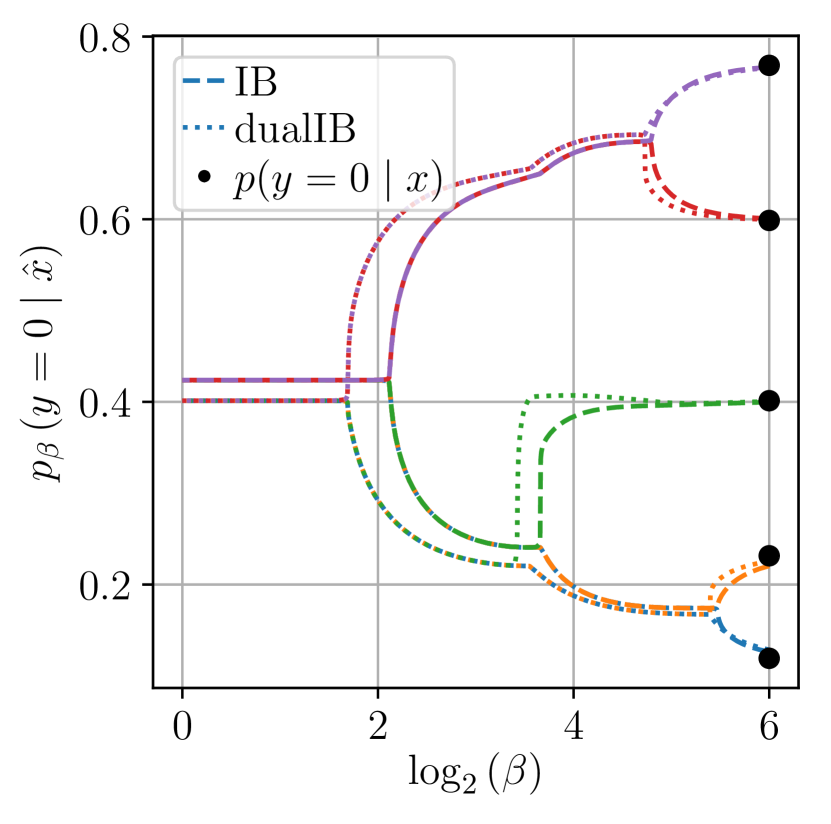
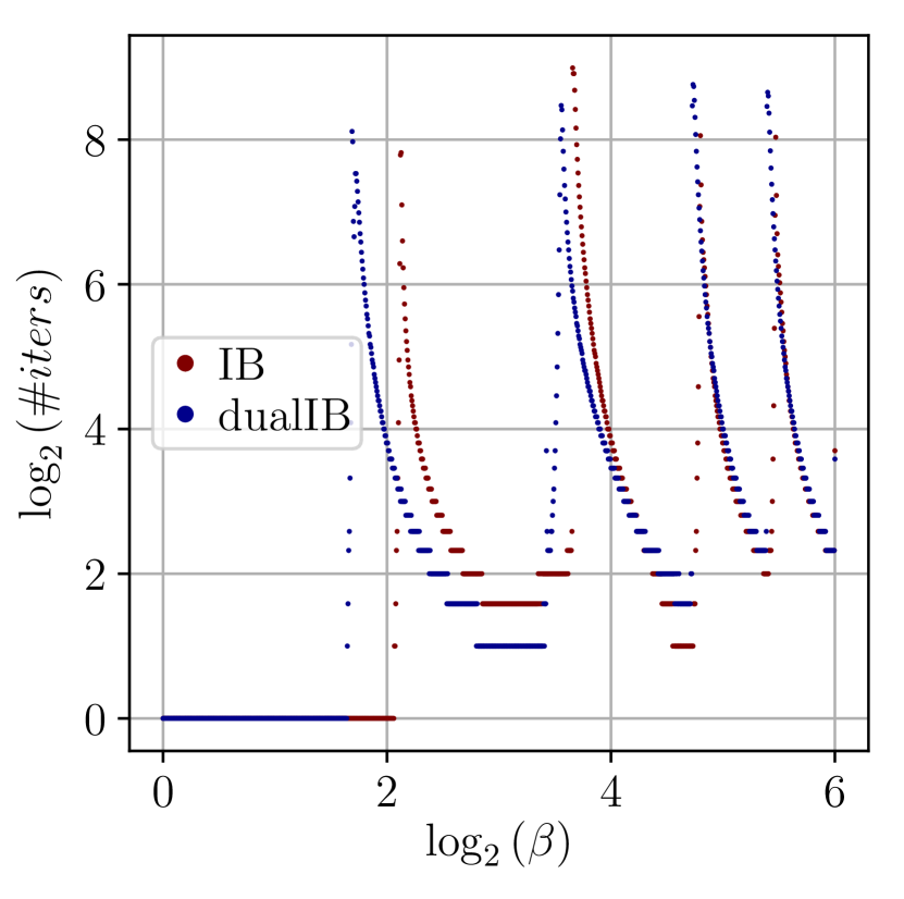
From Theorem 4 we deduce that as the dimensionality of the problem increases (implying the number of critical points grows) the dualIB’s approximation of the IB’s information plane becomes tighter. We illustrate the behavior of the dualIB’s solutions in comparison to the IB’s on a low-dimensional problem that is easy to analyze and visualize, with a binary Yπ‘ŒY and only 555 possible inputs X𝑋X (the complete definition is given in Β§D.1). For any given β𝛽\beta, the encoder-decoder iterations converge to stationary solutions of the dualIB or IB equations. The evolution of the optimal decoder, pβ​\brkβˆ—y=0∣x^subscript𝑝𝛽\brk𝑦conditional0^π‘₯p_{\beta}\brk*{y=0\mid\hat{x}}, βˆ€x^∈X^for-all^π‘₯^𝑋\forall\hat{x}\in\hat{X}, as a function of β𝛽\beta, forms a bifurcation diagram (FigureΒ 1(a)), in which the critical points define the location of the bifurcation. At the critical points the number of iterations diverges (FigureΒ 1(b)). While the overall structure of the solutions is similar, we see a β€œshift” in the appearance of the representation splits between the two frameworks. Specifically, as predicted by Theorem 4 the dualIB bifurcations occur at lower β𝛽\beta values than those of the IB. The inset of FigureΒ 1(c) depicts this comparison between the two information curves. While we know that IyIB​\brkβˆ—Ξ²subscriptsuperscript𝐼IB𝑦\brk𝛽I^{\rm{IB}}_{y}\brk*{\beta} is always larger, we see that for this setting the two curves are almost indistinguishable. Looking at Iysubscript𝐼𝑦I_{y} as a function of β𝛽\beta (FigureΒ 1(c)) the importance of the critical points is revealed as the corresponding cusps along these curves correspond to β€œjumps” in the accessible information. Furthermore, the distance between the curves is minimized precisely at the dual critical points, as predicted by the theory.
Refer to caption
(a) The bifurcation diagram
Refer to caption
(b) Convergence Time
Refer to caption
(c) The information plane
Figure 1: \brk​a\brkπ‘Ž\brk{a} The bifurcation diagram; each color corresponds to one component of the representation x^∈X^^π‘₯^𝑋\hat{x}\in\hat{X} and depicts the decoder pβ​\brkβˆ—y=0∣x^subscript𝑝𝛽\brk𝑦conditional0^π‘₯p_{\beta}\brk*{y=0\mid\hat{x}}. Dashed lines represent the IB’s solution and dotted present the dualIB’s. The black dots denote the input distribution p​\brkβˆ—y=0∣x𝑝\brk𝑦conditional0π‘₯p\brk*{y=0\mid x}. \brkβˆ—b\brk𝑏\brk*{b} Convergence time the BA algorithms as a function of β𝛽\beta. \brkβˆ—c\brk𝑐\brk*{c} The desired label Information IyIB​\brkβˆ—Ξ²subscriptsuperscript𝐼IB𝑦\brk𝛽I^{\rm{IB}}_{y}\brk*{\beta} and IydualIB​\brkβˆ—Ξ²subscriptsuperscript𝐼dualIB𝑦\brk𝛽I^{\rm{dualIB}}_{y}\brk*{\beta} as functions of β𝛽\beta. The inset shows the information plane, Iysubscript𝐼𝑦I_{y} vs. Ixsubscript𝐼π‘₯I_{x}. The black dots are the dualIB’s critical points, Ξ²cdualIBsubscriptsuperscript𝛽dualIB𝑐\beta^{\rm{dualIB}}_{c}, and the grey triangles are the IB’s, Ξ²cIBsubscriptsuperscript𝛽IB𝑐\beta^{\rm{IB}}_{c}

4 The Exponential Family dualIB

One of the major drawbacks of the IB is that it fails to capture an existing parameterization of the data, that act as minimal sufficient statistics for it. Exponential families are the class of parametric distributions for which minimal sufficient statistics exist, forming an elegant theoretical core of parametric statistics and often emerge as maximum entropy [19] or stochastic equilibrium distributions, subject to observed expectation constraints. As the IB ignores the structure of the distribution, given data from an exponential family it won’t consider these known features. Contrarily, the dualIB accounts for this structure and its solution are given in terms of these features, defining the dualExpIB equations.

We consider the case in which the rule distribution is of the form, p​\brkβˆ—y∣x=eβˆ’βˆ‘r=0dΞ»r​(y)​Ar​(x)conditional𝑝\brk𝑦π‘₯superscript𝑒superscriptsubscriptπ‘Ÿ0𝑑superscriptπœ†π‘Ÿπ‘¦subscriptπ΄π‘Ÿπ‘₯p\brk*{y\mid x}=e^{-\sum_{r=0}^{d}\lambda^{r}(y)A_{r}(x)}, where Ar​(x)subscriptπ΄π‘Ÿπ‘₯A_{r}(x) are d𝑑d functions of the input xπ‘₯x and Ξ»r​(y)superscriptπœ†π‘Ÿπ‘¦\lambda^{r}(y) are functions of the label y𝑦y, or the parameters of this exponential family 222 The normalization factors, Zπ’šβˆ£π’™β€‹\brkβˆ—xsubscript𝑍conditionalπ’šπ’™\brkπ‘₯Z_{\boldsymbol{y}\mid\boldsymbol{x}}\brk*{x}, are written, for brevity, as λ𝒙0≑log⁑(βˆ‘y∏r=1deβˆ’Ξ»r​\brkβˆ—y​Ar​\brkβˆ—x)superscriptsubscriptπœ†π’™0subscript𝑦superscriptsubscriptproductπ‘Ÿ1𝑑superscript𝑒superscriptπœ†π‘Ÿ\brk𝑦subscriptπ΄π‘Ÿ\brkπ‘₯\lambda_{\boldsymbol{x}}^{0}\equiv\log(\sum_{y}\prod_{r=1}^{d}e^{-{\lambda}^{r}\brk*{y}A_{r}\brk*{x}}) with A0​\brkβˆ—x≑1subscript𝐴0\brkπ‘₯1A_{0}\brk*{x}\equiv 1. We do not constrain the marginal p​\brkβˆ—x𝑝\brkπ‘₯p\brk*{x}.. For exponential forms the mutual information, I​(X;Y)πΌπ‘‹π‘ŒI(X;Y), is fully captured by the d𝑑d conditional expectations. This implies that all the relevant information (in the training sample) is captured by d𝑑d-dimensional empirical expectations which can lead to a reduction in computational complexity.

Next we show that for the dualIB, for all values of β𝛽\beta, this dimension reduction is preserved or improved along the dual information curve. The complete derivations are given in Β§F.

Theorem 5.

(dualExpIB) For data from an exponential family the optimal encoder-decoder of the dualIB are given by:

pβ​\brkβˆ—x^∣xconditionalsubscript𝑝𝛽\brk^π‘₯π‘₯\displaystyle p_{\beta}\brk*{\hat{x}\mid x} =pβ​\brkβˆ—x^​eβ​λβ0​\brkβˆ—x^Z𝒙^βˆ£π’™β€‹\brkβˆ—x;β​eβˆ’Ξ²β€‹βˆ‘r=1dλβr​\brkβˆ—x^​\brk​[s]βˆ—Ar​\brkβˆ—xβˆ’Ar,β​\brkβˆ—x^absentsubscript𝑝𝛽\brk^π‘₯superscript𝑒𝛽subscriptsuperscriptπœ†0𝛽\brk^π‘₯subscript𝑍conditional^𝒙𝒙\brkπ‘₯𝛽superscript𝑒𝛽superscriptsubscriptπ‘Ÿ1𝑑superscriptsubscriptπœ†π›½π‘Ÿ\brk^π‘₯\brkdelimited-[]𝑠subscriptπ΄π‘Ÿ\brkπ‘₯subscriptπ΄π‘Ÿπ›½\brk^π‘₯\displaystyle=\frac{p_{\beta}\brk*{\hat{x}}e^{\beta{\lambda}^{0}_{\beta}\brk*{\hat{x}}}}{Z_{\hat{\boldsymbol{x}}\mid\boldsymbol{x}}\brk*{x;\beta}}e^{-\beta\sum_{r=1}^{d}{\lambda}_{\beta}^{r}\brk*{\hat{x}}\brk[s]*{A_{r}\brk*{x}-A_{r,\beta}\brk*{\hat{x}}}}
pβ​\brkβˆ—y∣x^conditionalsubscript𝑝𝛽\brk𝑦^π‘₯\displaystyle p_{\beta}\brk*{y\mid\hat{x}} =eβˆ’βˆ‘r=1dΞ»r​\brkβˆ—y​Ar,β​\brkβˆ—x^βˆ’Ξ»Ξ²0​(x^),λβ0​(x^)=log⁑(βˆ‘yeβˆ’βˆ‘r=1dΞ»r​\brkβˆ—y​Ar,β​\brkβˆ—x^),formulae-sequenceabsentsuperscript𝑒superscriptsubscriptπ‘Ÿ1𝑑superscriptπœ†π‘Ÿ\brk𝑦subscriptπ΄π‘Ÿπ›½\brk^π‘₯subscriptsuperscriptπœ†0𝛽^π‘₯subscriptsuperscriptπœ†0𝛽^π‘₯subscript𝑦superscript𝑒superscriptsubscriptπ‘Ÿ1𝑑superscriptπœ†π‘Ÿ\brk𝑦subscriptπ΄π‘Ÿπ›½\brk^π‘₯\displaystyle=e^{-\sum_{r=1}^{d}\lambda^{r}\brk*{y}A_{r,\beta}\brk*{\hat{x}}-\lambda^{0}_{\beta}(\hat{x})}~{},~{}~{}~{}\lambda^{0}_{\beta}(\hat{x})=\log(\sum_{y}e^{-\sum_{r=1}^{d}\lambda^{r}\brk*{y}A_{r,\beta}\brk*{\hat{x}}}), (8)

with the constraints and multipliers expectations,

Ar,β​\brkβˆ—x^subscriptπ΄π‘Ÿπ›½\brk^π‘₯\displaystyle A_{r,\beta}\brk*{\hat{x}} β‰‘βˆ‘xpβ​\brkβˆ—x∣x^​Ar​\brkβˆ—x,λβr​\brkβˆ—x^β‰‘βˆ‘ypβ​\brkβˆ—y∣x^​λr​\brkβˆ—y,1≀r≀d.absentconditionalsubscriptπ‘₯subscript𝑝𝛽\brkπ‘₯^π‘₯subscriptπ΄π‘Ÿ\brkπ‘₯subscriptsuperscriptπœ†π‘Ÿπ›½\brk^π‘₯conditionalsubscript𝑦subscript𝑝𝛽\brk𝑦^π‘₯superscriptπœ†π‘Ÿ\brk𝑦1π‘Ÿπ‘‘\displaystyle\equiv\sum_{x}p_{\beta}\brk*{x\mid\hat{x}}A_{r}\brk*{x}~{},~{}\lambda^{r}_{\beta}\brk*{\hat{x}}\equiv\sum_{y}p_{\beta}\brk*{y\mid\hat{x}}\lambda^{r}\brk*{y}~{},~{}1\leq r\leq d~{}. (9)

This defines a simplified iterative algorithm for solving the dualExpIB problem. Given the mapping of x∈Xπ‘₯𝑋x\in X to \brk​[c]βˆ—Ar​\brkβˆ—xr=1d\brkdelimited-[]𝑐subscriptπ΄π‘Ÿ\brksuperscriptsubscriptπ‘₯π‘Ÿ1𝑑\brk[c]*{A_{r}\brk*{x}}_{r=1}^{d} the problem is completely independent of xπ‘₯x and we can work in the lower dimensional embedding of the features, Ar​\brkβˆ—xsubscriptπ΄π‘Ÿ\brkπ‘₯A_{r}\brk*{x}. Namely, the update procedure is reduced to the dimensions of the sufficient statistics. Moreover, the representation is given in terms of the original features, a desirable feature for any model based problem.

5 Optimizing the error exponent

The dualIB optimizes an upper bound on the error exponent of the representation multi class testing problem. The error exponent accounts for the decay of the prediction error as a function of data size n𝑛n. This implies the dualIB tends to minimize the prediction error. For the classical binary hypothesis testing, the classification Bayes error, Pe(n)subscriptsuperscript𝑃𝑛𝑒P^{(n)}_{e}, is the weighted sum of type 1 and type 2 errors. For large n𝑛n, both errors decay exponentially with the test size n𝑛n, and the best error exponent, Dβˆ—superscript𝐷D^{*}, is given by the Chernoff information. The Chernoff information is also a measure of distance defined as, C​\brkβˆ—p0,p1=min0<Ξ»<1⁑\brk​[c]βˆ—logβ€‹βˆ‘xp0λ​\brkβˆ—x​p11βˆ’Ξ»β€‹\brkβˆ—x𝐢\brksubscript𝑝0subscript𝑝1subscript0πœ†1\brkdelimited-[]𝑐subscriptπ‘₯superscriptsubscript𝑝0πœ†\brkπ‘₯superscriptsubscript𝑝11πœ†\brkπ‘₯C\brk*{p_{0},p_{1}}=\min_{0<\lambda<1}\brk[c]*{\log\sum_{x}p_{0}^{\lambda}\brk*{x}p_{1}^{1-\lambda}\brk*{x}}, and we can understand it as an optimization on the log\log-partition function of pΞ»subscriptπ‘πœ†p_{\lambda} to obtain Ξ»πœ†\lambda (for further information see [13] and Β§G).

The intuition behind the optimization of Dβˆ—superscript𝐷D^{*} by the dualIB is in its distortion, the order of the prediction and the observation which implies the use of geometrical mean. The best achievable exponent (see [13]) in Bayesian probability of error is given by the KL-distortion between pΞ»βˆ—subscript𝑝superscriptπœ†p_{\lambda^{*}} (∝p0Ξ»βˆ—β€‹\brkβˆ—x​p11βˆ’Ξ»βˆ—β€‹\brkβˆ—xproportional-toabsentsuperscriptsubscript𝑝0superscriptπœ†\brkπ‘₯superscriptsubscript𝑝11superscriptπœ†\brkπ‘₯\propto p_{0}^{\lambda^{*}}\brk*{x}p_{1}^{1-\lambda^{*}}\brk*{x}) to p0subscript𝑝0p_{0} or p1subscript𝑝1p_{1}, such that pΞ»βˆ—subscript𝑝superscriptπœ†p_{\lambda^{*}} is the mid point between p0subscript𝑝0p_{0} and p1subscript𝑝1p_{1} on the geodesic of their geometric means. By mapping the dualIB decoder to Ξ»πœ†\lambda, it follows that the above minimization is proportional to the log\log-partition function of pβ​\brkβˆ—x∣x^conditionalsubscript𝑝𝛽\brkπ‘₯^π‘₯p_{\beta}\brk*{x\mid\hat{x}}, namely we obtain the mapping pβ​\brkβˆ—x∣x^=pΞ»conditionalsubscript𝑝𝛽\brkπ‘₯^π‘₯subscriptπ‘πœ†p_{\beta}\brk*{x\mid\hat{x}}=p_{\lambda}.

In the generalization to multi class classification the error exponent is given by the pair of hypotheses with the minimal Chernoff information [20]. However, finding this value is generally difficult as it requires solving for each pair in the given classes. Thus, we consider an upper bound to it, the mean of the Chernoff information terms over classes. The representation variable adds a new dimension on which we average on and we obtain a bound on the optimal (in expectation over x^^π‘₯\hat{x}) achievable exponent, D^Ξ²=minpΞ²\brkβˆ—y∣x^,pΞ²\brkβˆ—x^∣x⁑𝔼pβ​\brkβˆ—y,x^​\brk​[s]βˆ—D​\brk​[s]βˆ—pβ​\brkβˆ—xβ€‹βˆ£x^βˆ£β€‹p​\brkβˆ—x∣y\hat{D}_{\beta}=\min_{p_{\beta}\brk*{y\mid\hat{x}},p_{\beta}\brk*{\hat{x}\mid x}}\mathbb{E}_{p_{\beta}\brk*{y,\hat{x}}}\brk[s]*{D\brk[s]*{p_{\beta}\brk*{x\mid\hat{x}}\mid p\brk*{x\mid y}}}. This expression is bounded from above by the dualIB minimization problem. Thus, the dualIB (on expectation) minimizes the prediction error for every n𝑛n. A formal derivation of the above along with an analytical example of a multi class classification problem is given in Β§G. In Β§6.1.3 we experimentally demonstrate that this also holds for a variational dualIB framework using a DNN.

6 Variational Dual Information Bottleneck

The Variational Information Bottleneck (VIB) approach introduced by Alemi et al. [5] allows to parameterize the IB model using Deep Neural Networks (DNNs). The variational bound of the IB is obtained using DNNs for both the encoder and decoder. Since then, various extensions have been made [21, 22] demonstrating promising attributes. Recently, along this line, the Conditional Entropy Bottleneck (CEB) [23] was proposed. The CEB provides variational optimizing bounds on I​(Y;X^)πΌπ‘Œ^𝑋I(Y;\hat{X}), I​(X;X^)𝐼𝑋^𝑋I(X;\hat{X}) using a variational decoder q​\brkβˆ—y∣x^conditionalπ‘ž\brk𝑦^π‘₯q\brk*{y\mid\hat{x}}, variational conditional marginal, q​\brkβˆ—x^∣yconditionalπ‘ž\brk^π‘₯𝑦q\brk*{\hat{x}\mid y}, and a variational encoder, p​\brkβˆ—x^∣xconditional𝑝\brk^π‘₯π‘₯p\brk*{\hat{x}\mid x}, all implemented by DNNs.

Here, we present the variational dualIB (VdualIB), which optimizes the variational dualIB objective for using in DNNs. Following the CEB formalism, we bound the dualIB objective. We develop a variational form of the dualIB distortion and combine it with the bound for I​(X;X^)𝐼𝑋^𝑋I(X;\hat{X}) (as in the CEB). This gives us the following Theorem (for the proof see Β§H.1.).

Theorem 6.

The VdualIB objective is given by:

minq\brkβˆ—x^∣y,p\brkβˆ—x^∣x⁑\brk​[c]βˆ—π”Όp~​\brkβˆ—yβ€‹βˆ£x​p​\brkβˆ—x^βˆ£β€‹x​p​\brkβˆ—x​\brk​[s]βˆ—log⁑p​\brkβˆ—x^∣xq​\brkβˆ—x^∣y+β​𝔼p​\brkβˆ—yβ€‹βˆ£x^​p​\brkβˆ—x^βˆ£β€‹x​\brk​[s]βˆ—log⁑p​\brkβˆ—y∣x^p~​\brkβˆ—y∣x,\displaystyle\min_{q\brk*{\hat{x}\mid y},p\brk*{\hat{x}\mid x}}\brk[c]*{\mathbb{E}_{\tilde{p}\brk*{y\mid x}p\brk*{\hat{x}\mid x}p\brk*{x}}\brk[s]*{\log\frac{p\brk*{\hat{x}\mid x}}{q\brk*{\hat{x}\mid y}}}+\beta\mathbb{E}_{p\brk*{y\mid\hat{x}}p\brk*{\hat{x}\mid x}}\brk[s]*{\log\frac{p\brk*{y\mid\hat{x}}}{\tilde{p}\brk*{y\mid x}}}}, (10)

where p~​\brkβˆ—y∣xconditional~𝑝\brk𝑦π‘₯\tilde{p}\brk*{y\mid x} is a distribution based on the given labels of the data-set, which we relate to as the noise model. Under the assumption that the noise model captures the distribution of the data the above provides a variational upper bound to the dualIB functional (4).

Due to the nature of its objective the dualIB requires a noise model. We must account for the contribution to the objective arising from p~​\brkβˆ—y∣xconditional~𝑝\brk𝑦π‘₯\tilde{p}\brk*{y\mid x} which could be ignored in the VIB case. The noise model can be specified by its assumptions over the data-set. In Β§6.1.2 we elaborate on possible noise models choices and their implications on the performance. Notice that the introduction of p~​(y∣x)~𝑝conditional𝑦π‘₯\tilde{p}(y\mid x) implies that, unlike most machine learning models, the VdualIB does not optimize directly the error between the predicted and desired labels in the training data. Instead, it does so implicitly with respect to the noisy training examples. This is not unique to the VdualIB, as it is equivalent to training with noisy labels, often done to prevent over-fitting. For example, in [24] the authors show that label noise can improve generalization that results in a reduction in the mutual information between the input and the output.

In practice, similarly to the CEB, for the stochastic encoder, p​(x^∣x)𝑝conditional^π‘₯π‘₯p(\hat{x}\mid x), we use the original architecture, replacing the final softmax layer with a linear dense layer with d𝑑d outputs. These outputs are taken as the means of a multivariate Gaussian distribution with unit diagonal covariance. For the variational decoder, q​(y∣x^)π‘žconditional𝑦^π‘₯q(y\mid\hat{x}), any classifier network can be used. We take a linear softmax classifier which takes the encoder as its input. The reverse decoder q​(x^∣y)π‘žconditional^π‘₯𝑦q(\hat{x}\mid y) is implemented by a network which maps a one-hot representation of the labels to the d𝑑d-dimensional output interpreted as the mean of the corresponding Gaussian marginal.

6.1 Experiments

To investigate the VdualIB on real-world data we compare it to the CEB model using a DNN over two data-sets, FasionMNIST and CIFAR10. For both, we use a Wide ResNet 28βˆ’10281028-10 [25] as the encoder, a one layer Gaussian decoder and a single layer linear network for the reverse decoder (similarly to the setup in [26]). We use the same architecture to train networks with VdualIB and VIB objectives. (See Β§H.2 for details on the experimental setup). We note that in our attempts to train over the CIFAR100 data-set the results did not fully agree with the results on the above data-sets (for more information see Β§H.5). An open source implementation is available here.

6.1.1 The variational information plane

As mentioned, the information plane describes the compression-prediction trade-off. It enables us to compare different models and evaluate their β€œbest prediction level” in terms of the desired label information, for each compression level. In [26] the authors provide empirical evidence that information bottlenecking techniques can improve both generalization and robustness. Other works [23, 27, 28] provide both theoretical and conceptual insights into why these improvements occur.

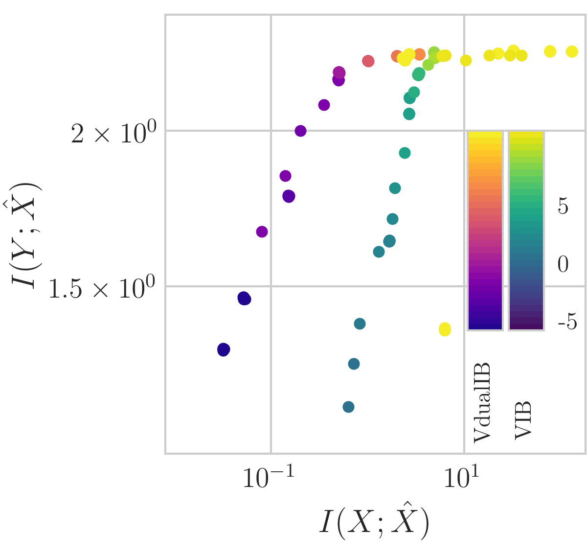
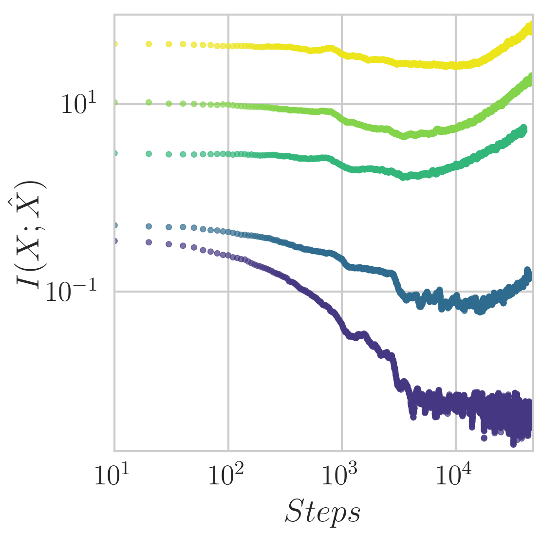
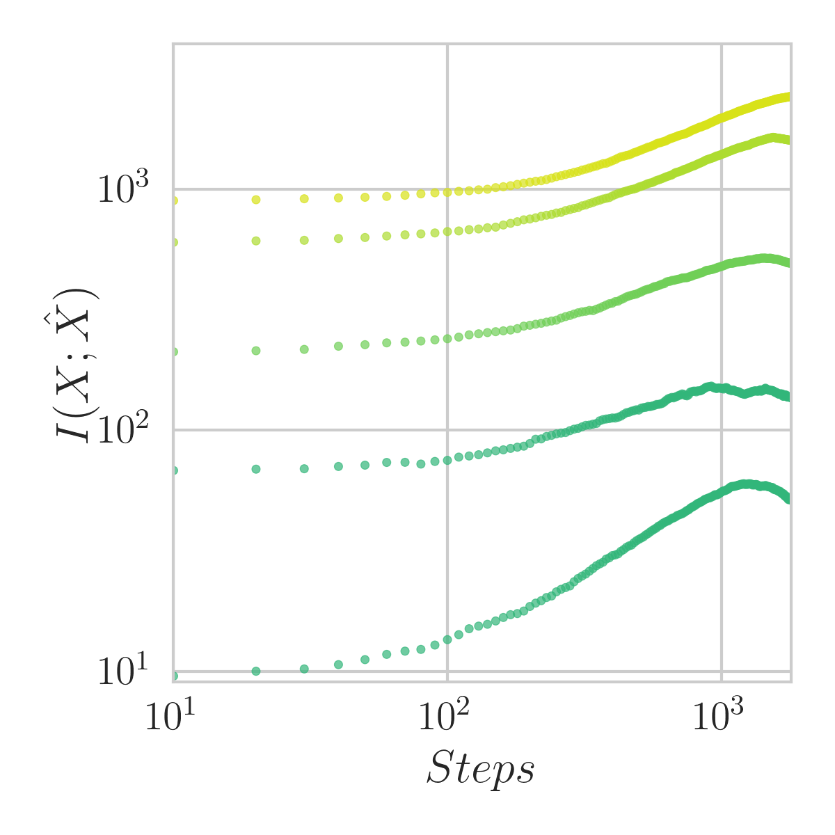
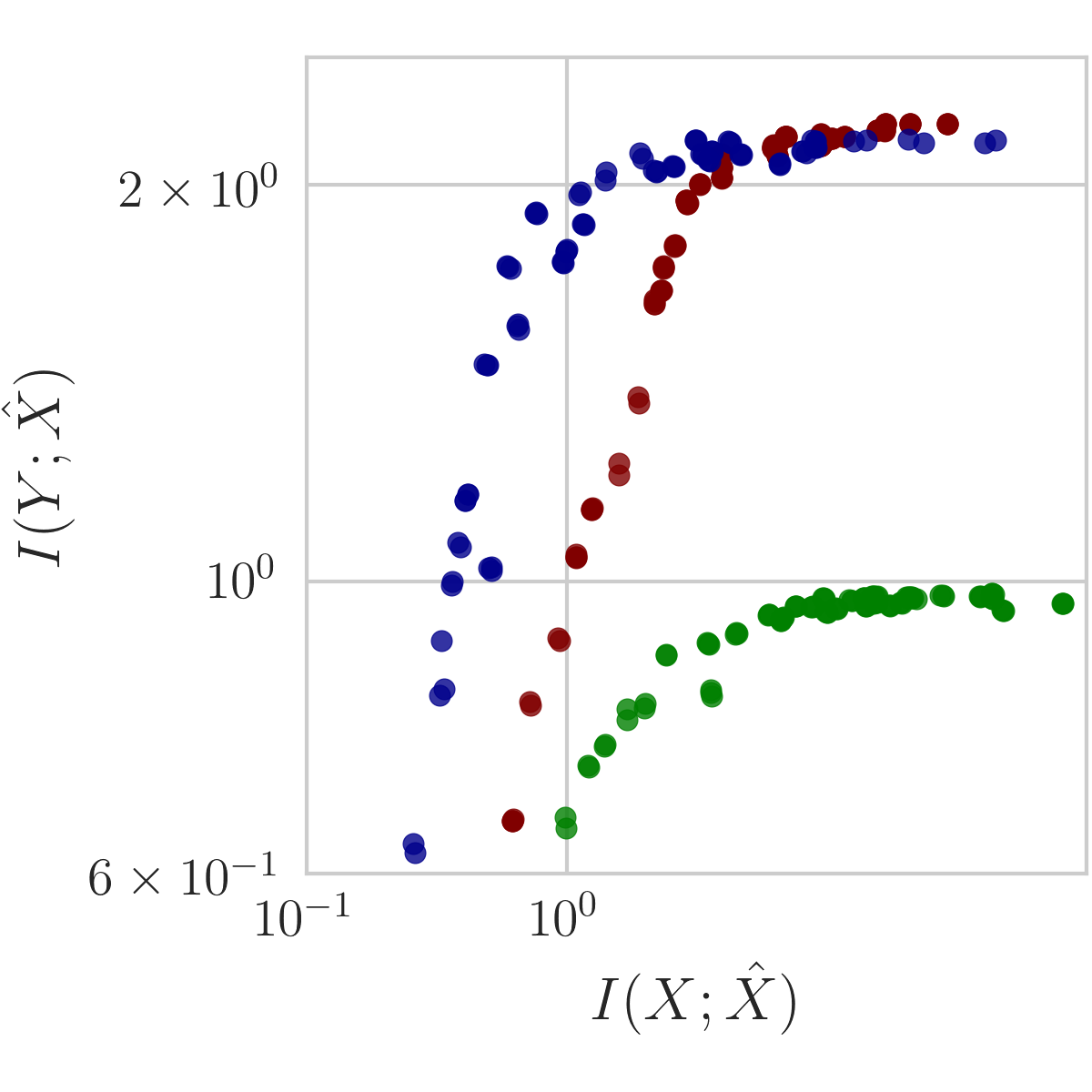
In FigureΒ 2 we present the information plane of the VdualIB where the distribution p~​\brkβˆ—y∣xconditional~𝑝\brk𝑦π‘₯\tilde{p}\brk*{y\mid x} (the noise model) is a learnt confusion matrix, ConfVdualIB (similarly to [11]). We compare it to the VIB over a range of β𝛽\beta values (βˆ’5≀log⁑β≀55𝛽5-5\leq\log{\beta}\leq 5). FigureΒ 2(a) validates that, as expected, the information growth is approximately monotonic with β𝛽\beta. Comparing the VdualIB to the VIB model, we can see significant differences between their representations. The VdualIB successfully obtains better compressed representations in comparison to the VIB performance, where only for large values of I​(X;X^)𝐼𝑋^𝑋I(X;\hat{X}) their performances match. As predicted by the theory, in the limit Ξ²β†’βˆžβ†’π›½\beta\rightarrow\infty the models behaviour match. Furthermore, the VdualIB values are smoother and they are spread over the information plane, making it easier to optimize for a specific value in it. In FigureΒ 2(b) we consider the dynamics of I​(X;X^)𝐼𝑋^𝑋I(X;\hat{X}) for several values of β𝛽\beta. Interestingly, at the initial training stage the representation information for all values of β𝛽\beta decreases. However, as the training continues, the information increases only for high β𝛽\betas.

Refer to caption
(a) The information plane
Refer to caption
(b) I​(X;X^)𝐼𝑋^𝑋I(X;\hat{X}) vs. update steps
Refer to caption
(c) Accuracy vs. training size
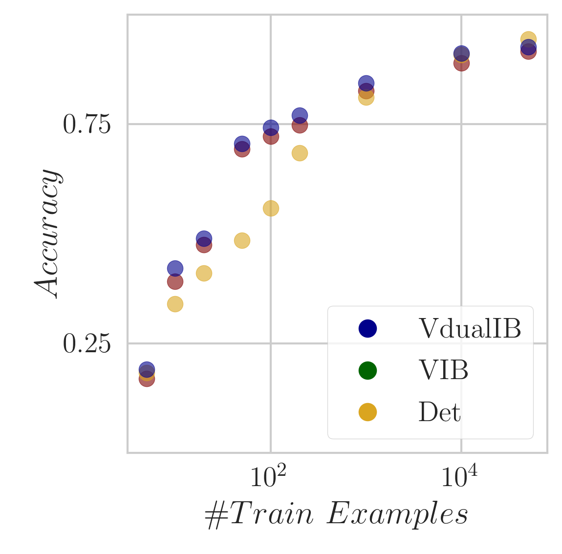
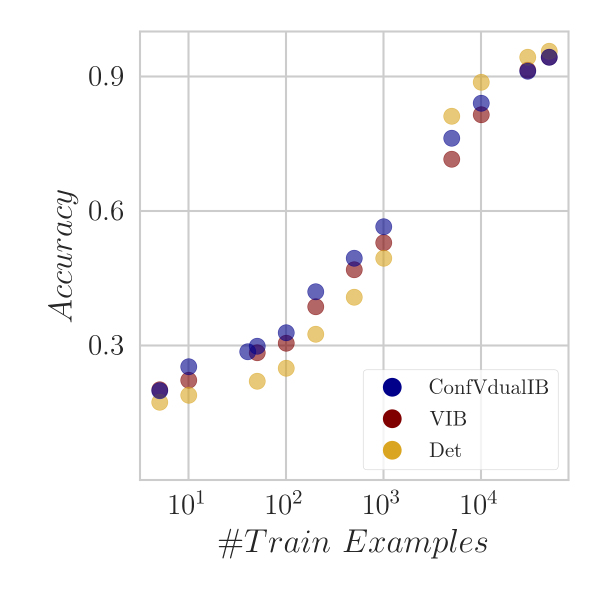
Figure 2: Experiments over FashionMNIST. (a)π‘Ž(a) The information plane of the ConfVdualIB and VIB for a range of β𝛽\beta values at the final training step. (b)𝑏(b) The evolution of the the ConfVdualIB’s I​(X;X^)𝐼𝑋^𝑋I(X;\hat{X}) along the optimization update steps. (c)𝑐(c) The models accuracy as a function of the training set size.

6.1.2 The VdualIB noise model

As mentioned above, learning with the VdualIB objective requires a choice of a noise model for the distribution p~​\brkβˆ—y∣x^conditional~𝑝\brk𝑦^π‘₯\tilde{p}\brk*{y\mid\hat{x}}. To explore the influence of different models on the learning we evaluate four types, with different assumptions on the access to the data. (i) Adding Gaussian noise to the one-hot vector of the true label (GVdualIB); (ii) An analytic Gaussian integration of the log-loss around the one-hot labels; (iii) A pre-computed confusion matrix for the labels (ConfVdualIB) as in [11]; (iv) Using predictions of another trained model as the induced distribution. Where for (i) and (ii) the variance acts as a free parameter determining the noise level. The complexity of the noise models can be characterized by the additional prior knowledge on our data-set they require. While adding Gaussian noise does not require prior knowledge, using a trained model requires access to the prediction for every data sample. The use of a confusion matrix is an intermediate level of prior knowledge requiring access only to the \abs​𝒴×\abs​𝒴\abs𝒴\abs𝒴\abs{\mathcal{Y}}\times\abs{\mathcal{Y}} pre-computed matrix. Here we present cases (i) and (iii) (see Β§H.4 for (ii) and (iv)). Note that although using the VIB does not require the use of a noise model we incorporate it by replacing the labels with p~​\brkβˆ—y∣xconditional~𝑝\brk𝑦π‘₯\tilde{p}\brk*{y\mid x}. In the analysis below, the results are presented with the VIB trained with the same noise model as the VdualIB (see Β§H.4 for a comparison between training VdualIB with noise and VIB without it).

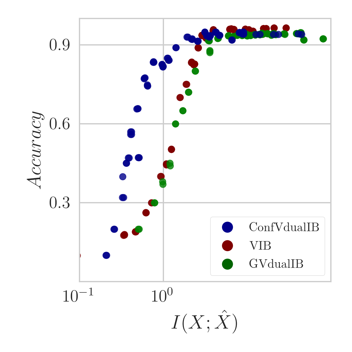
FigureΒ 3 depicts the information plane of the CIFAR10 data-set. FigureΒ 3(a) shows the information obtained from a range of β𝛽\beta. The colors depict the different models ConfVdualIB, GVdualIB and the VIB. As we can see, training a VdualIB with Gaussian noise achieves much less information with the labels at any given I​(X;X^)𝐼𝑋^𝑋I(X;\hat{X}). We note that we verified that this behaviour is consistent over a wide range of variances. The ConfVdualIB model performance is similar to the VIB’s with the former showcasing more compressed representations. When we present the prediction accuracy (FigureΒ 3(b)), here all models attain roughly the same accuracy values. The discrepancy between the accuracy and information, I​(Y;X^)πΌπ‘Œ^𝑋I(Y;\hat{X}), is similar to the one discussed in [29].
Refer to caption
(a) The information plane
Refer to caption
(b) Accuracy vs. I​(X;X^)𝐼𝑋^𝑋I(X;\hat{X})
Refer to caption
(c) Accuracy vs. training size
Figure 3: Experiments over CIFAR10. (a)π‘Ž(a) The information plane of the VIB, ConfVdualIB, GVdualIB and VIB for a range of β𝛽\beta values. (b)𝑏(b) The accuracy of the models as a function of the mutual information, I​(X;X^)𝐼𝑋^𝑋I(X;\hat{X}). (c)𝑐(c) The accuracy of the models as a function of the training set size.

6.1.3 Performance with different training set sizes

Our theoretical analysis (Β§5) shows that under given assumptions the dualIB bounds the optimal achievable error exponent on expectation hence it optimizes the error for a given data size n𝑛n. We turn to test this in the VdualIB setting. We train the models on a subset of the training set and evaluate them on the test set. We compare the VIB and the VdualIB to a deterministic network (Det; Wide Res Net 28-10). Both the VIB and VdualIB are trained over a wide range of β𝛽\beta values (βˆ’5≀log⁑β≀65𝛽6-5\leq\log{\beta}\leq 6). Presented is the best accuracy value for each model at a given n𝑛n. FigureΒ 2(c) and FigureΒ 3(c) show the accuracy of the models as a function of the training set size over FashionMNIST and CIFAR10 respectively. The VdualIB performance is slightly better in comparison to the VIB, while the accuracy of the deterministic network is lower for small training sets. The superiority of the variational models over the deterministic network is not surprising as minimizing I​(X;X^)𝐼𝑋^𝑋I(X;\hat{X}) acts as regularization.

7 Conclusions

We present here the Dual Information Bottleneck (dualIB), a framework resolving some of the known drawbacks of the IB obtained by a mere switch between the terms in the distortion function. We provide the dualIB self-consistent equations allowing us to obtain analytical solutions. A local stability analysis revealed the underlying structure of the critical points of the solutions, resulting in a full bifurcation diagram of the optimal pattern representations. The study of the dualIB objective reveals several interesting properties. First, when the data can be modeled in a parametric form the dualIB preserves this structure and it obtains the representation in terms of the original parameters, as given by the dualExpIB equations. Second, it optimizes the mean prediction error exponent thus improving the accuracy of the predictions as a function of the data size. In addition to the dualIB analytic solutions, we provide a variational dualIB (VdualIB) framework, which optimizes the functional using DNNs. This framework enables practical implementation of the dualIB to real world data-sets. While a broader analysis is required, the VdualIB experiments shown validate the theoretical predictions. Our results demonstrate the potential advantages and unique properties of the framework.

References

  • [1] Naftali Tishby, FernandoΒ C. Pereira, and William Bialek. The information bottleneck method. In Proc. of the 37-th Annual Allerton Conference on Communication, Control and Computing, pages 368–377, 1999.
  • [2] Shuang Ma, Daniel McDuff, and Yale Song. Unpaired image-to-speech synthesis with multimodal information bottleneck. In Proceedings of the IEEE International Conference on Computer Vision, pages 7598–7607, 2019.
  • [3] Elad Schneidman, Noam Slonim, Naftali Tishby, RΒ deRuyter van Steveninck, and William Bialek. Analyzing neural codes using the information bottleneck method. Advances in Neural Information Processing Systems, NIPS, 2001.
  • [4] XiangΒ Lisa Li and Jason Eisner. Specializing word embeddings (for parsing) by information bottleneck. In Proceedings of the 2019 Conference on Empirical Methods in Natural Language Processing and 9th International Joint Conference on Natural Language Processing, pages 2744–2754, Hong Kong, November 2019. Best Paper Award.
  • [5] AlexanderΒ A. Alemi, Ian Fischer, JoshuaΒ V. Dillon, and Kevin Murphy. Deep variational information bottleneck. ArXiv, abs/1612.00410, 2016.
  • [6] Sonali Parbhoo, Mario Wieser, and Volker Roth. Causal deep information bottleneck. ArXiv, abs/1807.02326, 2018.
  • [7] Ben Poole, Sherjil Ozair, Aaron vanΒ den Oord, AlexanderΒ A Alemi, and George Tucker. On variational bounds of mutual information. arXiv preprint arXiv:1905.06922, 2019.
  • [8] Ravid Shwartz-Ziv and Naftali Tishby. Opening the Black Box of Deep Neural Networks via Information. arXiv e-prints, page arXiv:1703.00810, Mar 2017.
  • [9] Charlie Nash, Nate Kushman, and ChristopherΒ KI Williams. Inverting supervised representations with autoregressive neural density models. arXiv preprint arXiv:1806.00400, 2018.
  • [10] Ziv Goldfeld, Ewout vanΒ den Berg, Kristjan Greenewald, Igor Melnyk, Nam Nguyen, Brian Kingsbury, and Yury Polyanskiy. Estimating information flow in deep neural networks. arXiv preprint arXiv:1810.05728, 2018.
  • [11] Tailin Wu and Ian Fischer. Phase transitions for the information bottleneck in representation learning. arXiv preprint arXiv:2001.01878, 2020.
  • [12] AlbertΒ E. Parker, TomΓ‘Ε‘ Gedeon, and AlexanderΒ G. Dimitrov. Annealing and the rate distortion problem. In S.Β Becker, S.Β Thrun, and K.Β Obermayer, editors, Advances in Neural Information Processing Systems 15, pages 993–976. MIT Press, 2003.
  • [13] ThomasΒ M. Cover and JoyΒ A. Thomas. Elements of Information Theory (Wiley Series in Telecommunications and Signal Processing). Wiley-Interscience, New York, NY, USA, 2006.
  • [14] Shai Shalev-Shwartz and Shai Ben-David. Understanding machine learning: From theory to algorithms. Cambridge university press, 2014.
  • [15] Noam Slonim, Nir Friedman, and Naftali Tishby. Multivariate information bottleneck. Neural Computation, 18(8):1739–1789, 2006. PMID: 16771652.
  • [16] Ohad Shamir, Sivan Sabato, and Naftali Tishby. Learning and generalization with the information bottleneck. Theor. Comput. Sci., 411:2696–2711, 2010.
  • [17] Domenico Felice and Nihat Ay. Divergence functions in information geometry. In Frank Nielsen and FrΓ©dΓ©ric Barbaresco, editors, Geometric Science of Information - 4th International Conference, GSI 2019, Toulouse, France, August 27-29, 2019, Proceedings, volume 11712 of Lecture Notes in Computer Science, pages 433–442. Springer, 2019.
  • [18] Ran Gilad-bachrach, Amir Navot, and Naftali Tishby. An information theoretic tradeoff between complexity and accuracy. In In Proceedings of the COLT, pages 595–609. Springer, 2003.
  • [19] E.Β T. Jaynes. Information theory and statistical mechanics. Phys. Rev., 106:620–630, May 1957.
  • [20] MΒ Brandon Westover. Asymptotic geometry of multiple hypothesis testing. IEEE transactions on information theory, 54(7):3327–3329, 2008.
  • [21] DJΒ Strouse and DavidΒ J Schwab. The deterministic information bottleneck. Neural computation, 29(6):1611–1630, 2017.
  • [22] Adar Elad, Doron Haviv, Yochai Blau, and Tomer Michaeli. Direct validation of the information bottleneck principle for deep nets. In Proceedings of the IEEE International Conference on Computer Vision Workshops, pages 0–0, 2019.
  • [23] Ian Fischer. The conditional entropy bottleneck. In URL openreview. net/forum, 2018.
  • [24] Rafael MΓΌller, Simon Kornblith, and GeoffreyΒ E Hinton. When does label smoothing help? In Advances in Neural Information Processing Systems, pages 4696–4705, 2019.
  • [25] Sergey Zagoruyko and Nikos Komodakis. Wide residual networks. arXiv preprint arXiv:1605.07146, 2016.
  • [26] Ian Fischer and AlexanderΒ A Alemi. Ceb improves model robustness. arXiv preprint arXiv:2002.05380, 2020.
  • [27] Alessandro Achille and Stefano Soatto. Emergence of invariance and disentanglement in deep representations. The Journal of Machine Learning Research, 19(1):1947–1980, 2018.
  • [28] Alessandro Achille and Stefano Soatto. Information dropout: Learning optimal representations through noisy computation. IEEE transactions on pattern analysis and machine intelligence, 40(12):2897–2905, 2018.
  • [29] MichaelΒ W Dusenberry, Ghassen Jerfel, Yeming Wen, Yi-an Ma, Jasper Snoek, Katherine Heller, Balaji Lakshminarayanan, and Dustin Tran. Efficient and scalable bayesian neural nets with rank-1 factors. arXiv preprint arXiv:2005.07186, 2020.
  • [30] LawrenceΒ D. Brown. Fundamentals of statistical exponential families with applications in statistical decision theory. Lecture Notes-Monograph Series, 9:i–279, 1986.
  • [31] Amichai Painsky and GregoryΒ W. Wornell. Bregman Divergence Bounds and the Universality of the Logarithmic Loss. arXiv e-prints, page arXiv:1810.07014, Oct 2018.
  • [32] G.Β Tusnady and I.Β Csiszar. Information geometry and alternating minimization procedures. Statistics & Decisions: Supplement Issues, 1:205–237, 1984.
  • [33] Noga Zaslavsky and Naftali Tishby. Deterministic annealing and the evolution of optimal information bottleneck representations. Preprint, 2019.
  • [34] JorgeΒ R Tredicce, GianΒ Luca Lippi, Paul Mandel, Basile Charasse, Aude Chevalier, and BΒ PicquΓ©. Critical slowing down at a bifurcation. American Journal of Physics, 72(6):799–809, 2004.
  • [35] DiederikΒ P Kingma and Jimmy Ba. Adam: A method for stochastic optimization. arXiv preprint arXiv:1412.6980, 2014.

Appendix

Appendix A The Information Bottleneck method

The Information Bottleneck (IB) trade off between the encoder and decoder mutual information values is defined by the minimization of the Lagrangian:

β„±\brk[s]βˆ—pΞ²\brkβˆ—x^∣x;pΞ²\brkβˆ—y∣x^=I(X;X^)βˆ’Ξ²I(Y;X^),\displaystyle\mathcal{F}\brk[s]*{p_{\beta}\brk*{\hat{x}\mid x};p_{\beta}\brk*{y\mid\hat{x}}}=I(X;\hat{X})-\beta I(Y;\hat{X})~{}, (11)

independently over the convex sets of the normalized distributions, \brk​[c]βˆ—pβ​\brkβˆ—x^∣xconditional\brkdelimited-[]𝑐subscript𝑝𝛽\brk^π‘₯π‘₯\brk[c]*{p_{\beta}\brk*{\hat{x}\mid x}}, \brk​[c]βˆ—pβ​\brkβˆ—x^\brkdelimited-[]𝑐subscript𝑝𝛽\brk^π‘₯\brk[c]*{p_{\beta}\brk*{\hat{x}}} and \brk​[c]βˆ—pβ​\brkβˆ—y∣x^conditional\brkdelimited-[]𝑐subscript𝑝𝛽\brk𝑦^π‘₯\brk[c]*{p_{\beta}\brk*{y\mid\hat{x}}}, given a positive Lagrange multiplier β𝛽\beta. As shown in [1, 16], this is a natural generalization of the classical concept of Minimal Sufficient Statistics [13], where the estimated parameter is replaced by the output variable Yπ‘ŒY and exact statistical sufficiency is characterized by the mutual information equality: I​(X^;Y)=I​(X;Y)𝐼^π‘‹π‘ŒπΌπ‘‹π‘ŒI(\hat{X};Y)=I(X;Y). The minimality of the statistics is captured by the minimization of I​(X;X^)𝐼𝑋^𝑋I(X;\hat{X}), due to the Data Processing Inequality (DPI). However, non-trivial minimal sufficient statistics only exist for very special parametric distributions known as exponential families [30]. Thus in general, the IB relaxes the minimal sufficiency problem to a continuous family of representations X^^𝑋\hat{X} which are characterized by the trade off between compression, I​(X;X^)≑IX𝐼𝑋^𝑋subscript𝐼𝑋I(X;\hat{X})\equiv I_{X}, and accuracy, I​(Y;X^)≑IYπΌπ‘Œ^𝑋subscriptπΌπ‘ŒI(Y;\hat{X})\equiv I_{Y}, along a convex line in the Information-Plane (IYsubscriptπΌπ‘ŒI_{Y} vs. IXsubscript𝐼𝑋I_{X}). When the rule p​(x,y)𝑝π‘₯𝑦p(x,y) is strictly stochastic, the convex optimal line is smooth and each point along the line is uniquely characterized by the value of β𝛽\beta. We can then consider the optimal representations x^=x^​(Ξ²)^π‘₯^π‘₯𝛽\hat{x}=\hat{x}(\beta) as encoder-decoder pairs: (pβ​(x∣x^),pβ​(y∣x^))subscript𝑝𝛽conditionalπ‘₯^π‘₯subscript𝑝𝛽conditional𝑦^π‘₯(p_{\beta}(x\mid\hat{x}),p_{\beta}(y\mid\hat{x}))333Here we use the inverse encoder, which is in the fixed dimension simplex of distributions over X𝑋X. - a point in the continuous manifold defined by the Cartesian product of these distribution simplexes. We also consider a small variation of these representations, δ​x^𝛿^π‘₯\delta\hat{x}, as an infinitesimal change in this (encoder-decoder) continuous manifold (not necessarily on the optimal line(s)).

A.1 IB and Rate-Distortion Theory

The IB optimization trade off can be considered as a generalized rate-distortion problem [13] with the distortion function between a data point, xπ‘₯x and a representation point x^^π‘₯\hat{x} taken as the KL-divergence between their predictions of the desired label y𝑦y:

dIB​\brkβˆ—x,x^subscript𝑑IB\brkπ‘₯^π‘₯\displaystyle d_{\rm{IB}}\brk*{x,\hat{x}} =D​\brk​[s]βˆ—p​\brkβˆ—yβ€‹βˆ£x|​|pβ​\brkβˆ—y|​x^absent𝐷\brkdelimited-[]𝑠𝑝\brk𝑦delimited-∣|π‘₯subscript𝑝𝛽\brk𝑦^π‘₯\displaystyle=D\brk[s]*{p\brk*{y\mid x}||p_{\beta}\brk*{y|\hat{x}}}
=βˆ‘yp​\brkβˆ—y∣x​log⁑p​\brkβˆ—y∣xpβ​\brkβˆ—y∣x^.absentconditionalsubscript𝑦𝑝\brk𝑦π‘₯conditional𝑝\brk𝑦π‘₯conditionalsubscript𝑝𝛽\brk𝑦^π‘₯\displaystyle=\sum_{y}p\brk*{y\mid x}\log\frac{p\brk*{y\mid x}}{p_{\beta}\brk*{y\mid\hat{x}}}. (12)

The expected distortion 𝔼pβ​(x,x^)​\brk​[s]βˆ—dIB​\brkβˆ—x,x^subscript𝔼subscript𝑝𝛽π‘₯^π‘₯\brkdelimited-[]𝑠subscript𝑑IB\brkπ‘₯^π‘₯\mathbb{E}_{p_{\beta}(x,\hat{x})}\brk[s]*{d_{\rm{IB}}\brk*{x,\hat{x}}} for the optimal decoder is simply the label-information loss: I​(X;Y)βˆ’I​(X^;Y)πΌπ‘‹π‘ŒπΌ^π‘‹π‘ŒI(X;Y)-I(\hat{X};Y), using the Markov chain condition. Thus minimizing the expected IBIB\rm{IB} distortion is equivalent to maximizing I​(X^;Y)𝐼^π‘‹π‘ŒI(\hat{X};Y), or minimizing (1). Minimizing this distortion is equivalent to minimizing the cross-entropy loss, and it provides an upper-bound to other loss functions such as the β„’1subscriptβ„’1\mathcal{L}_{1}-loss (due to the Pinsker inequality, see also [31]). Pinsker implies that both orders of the cross-entropy act as an upper bound to the β„’1subscriptβ„’1\mathcal{L}_{1}-loss, min{D\brk[s]βˆ—q||p,D\brk[s]βˆ—p||q}β‰₯12​log⁑2βˆ₯pβˆ’qβˆ₯12.\min\{D\brk[s]*{q||p},D\brk[s]*{p||q}\}\geq\frac{1}{2\log 2}\|p-q\|_{1}^{2}~{}.

A.2 The IB Equations

For discrete X𝑋X and Yπ‘ŒY, a necessary condition for the IBIB\rm{IB} (local) minimization is given by the three self-consistent equations for the optimal encoder-decoder pairs, known as the IB equations:

{\brkβˆ—ipβ​\brkβˆ—x^∣x=pβ​\brkβˆ—x^Z​\brkβˆ—x;β​eβˆ’Ξ²β€‹D​\brk​[s]βˆ—p​\brkβˆ—yβ€‹βˆ£x‖​pβ​\brkβˆ—y∣x^\brkβˆ—i​ipβ​\brkβˆ—x^=βˆ‘xpβ​\brkβˆ—x^∣x​p​\brkβˆ—x\brkβˆ—i​i​ipβ​\brkβˆ—y∣x^=βˆ‘xp​\brkβˆ—yβ€‹βˆ£x​pβ​\brkβˆ—xβˆ£β€‹x^,cases\brk𝑖conditionalsubscript𝑝𝛽\brk^π‘₯π‘₯subscript𝑝𝛽\brk^π‘₯𝑍\brkπ‘₯𝛽superscript𝑒conditional𝛽𝐷\brkdelimited-[]𝑠𝑝\brk𝑦delimited-βˆ£β€–π‘₯subscript𝑝𝛽\brk𝑦^π‘₯\brk𝑖𝑖subscript𝑝𝛽\brk^π‘₯conditionalsubscriptπ‘₯subscript𝑝𝛽\brk^π‘₯π‘₯𝑝\brkπ‘₯\brk𝑖𝑖𝑖conditionalsubscript𝑝𝛽\brk𝑦^π‘₯subscriptπ‘₯𝑝\brk𝑦delimited-∣∣π‘₯subscript𝑝𝛽\brkπ‘₯^π‘₯\displaystyle\begin{cases}\brk*{i}\ &p_{\beta}\brk*{\hat{x}\mid x}=\frac{p_{\beta}\brk*{\hat{x}}}{Z\brk*{x;\beta}}e^{-\beta D\brk[s]*{p\brk*{y\mid x}\|p_{\beta}\brk*{y\mid\hat{x}}}}\\ \brk*{ii}\ &p_{\beta}\brk*{\hat{x}}=\sum_{x}p_{\beta}\brk*{\hat{x}\mid x}p\brk*{x}\\ \brk*{iii}\ &p_{\beta}\brk*{y\mid\hat{x}}=\sum_{x}p\brk*{y\mid x}p_{\beta}\brk*{x\mid\hat{x}}\end{cases}, (13)

where Z​\brkβˆ—x;β𝑍\brkπ‘₯𝛽Z\brk*{x;\beta} is the normalization function. Iterating these equations is a generalized, Blahut-Arimoto, alternating projection algorithm [32, 13] and it converges to a stationary point of the Lagrangian, (1) [1]. Notice that the minimizing decoder, ((13)-(i​i​i)𝑖𝑖𝑖(iii)), is precisely the Bayes optimal decoder for the representation x^​(Ξ²)^π‘₯𝛽\hat{x}(\beta), given the Markov chain conditions.

A.3 Critical points and critical slowing down

One of the most interesting aspects of the IB equations is the existence of critical points along the optimal line of solutions in the information plane (i.e. the information curve). At these points the representations change topology and cardinality (number of clusters) [33, 12] and they form the skeleton of the information curve and representation space. To identify such points we perform a perturbation analysis of the IB equations:444We ignore here the possible interaction between the different representations, for simplicity.:

δ​log⁑pβ​\brkβˆ—x∣x^=conditional𝛿subscript𝑝𝛽\brkπ‘₯^π‘₯absent\displaystyle\delta\log p_{\beta}\brk*{x\mid\hat{x}}= Ξ²β€‹βˆ‘yp​\brkβˆ—yβ€‹βˆ£x​δ​log⁑pβ​\brkβˆ—yβˆ£β€‹x^,𝛽subscript𝑦𝑝\brk𝑦delimited-∣∣π‘₯𝛿subscript𝑝𝛽\brk𝑦^π‘₯\displaystyle\beta\sum_{y}p\brk*{y\mid x}\delta\log p_{\beta}\brk*{y\mid\hat{x}}, (14)
δ​log⁑pβ​\brkβˆ—y∣x^=1pβ​\brkβˆ—y∣x^β€‹βˆ‘xp​\brkβˆ—yβ€‹βˆ£x​pβ​\brkβˆ—xβˆ£β€‹x^​δ​log⁑pβ​\brkβˆ—x∣x^.conditional𝛿subscript𝑝𝛽\brk𝑦^π‘₯conditional1conditionalsubscript𝑝𝛽\brk𝑦^π‘₯subscriptπ‘₯𝑝\brk𝑦delimited-∣∣π‘₯subscript𝑝𝛽\brkπ‘₯^π‘₯𝛿subscript𝑝𝛽\brkπ‘₯^π‘₯\displaystyle\delta\log p_{\beta}\brk*{y\mid\hat{x}}=\frac{1}{p_{\beta}\brk*{y\mid\hat{x}}}\sum_{x}p\brk*{y\mid x}p_{\beta}\brk*{x\mid\hat{x}}\delta\log p_{\beta}\brk*{x\mid\hat{x}}. (15)

Substituting (15) into (14) and vice versa one obtains:

δ​log⁑pβ​\brkβˆ—x∣x^conditional𝛿subscript𝑝𝛽\brkπ‘₯^π‘₯\displaystyle\delta\log p_{\beta}\brk*{x\mid\hat{x}} =Ξ²β€‹βˆ‘y,xβ€²p​\brkβˆ—yβ€‹βˆ£x′​p​\brkβˆ—y∣xpβ​\brkβˆ—y∣x^​pβ​\brkβˆ—xβ€²βˆ£β€‹x^​δ​log⁑pβ​\brkβˆ—xβ€²βˆ£x^absentconditional𝛽subscript𝑦superscriptπ‘₯′𝑝\brk𝑦delimited-∣∣superscriptπ‘₯β€²conditional𝑝\brk𝑦π‘₯conditionalsubscript𝑝𝛽\brk𝑦^π‘₯subscript𝑝𝛽\brksuperscriptπ‘₯β€²^π‘₯𝛿subscript𝑝𝛽\brksuperscriptπ‘₯β€²^π‘₯\displaystyle=\beta\sum_{y,x^{\prime}}p\brk*{y\mid x^{\prime}}\frac{p\brk*{y\mid x}}{p_{\beta}\brk*{y\mid\hat{x}}}p_{\beta}\brk*{x^{\prime}\mid\hat{x}}\delta\log p_{\beta}\brk*{x^{\prime}\mid\hat{x}}
δ​log⁑pβ​\brkβˆ—y∣x^conditional𝛿subscript𝑝𝛽\brk𝑦^π‘₯\displaystyle\delta\log p_{\beta}\brk*{y\mid\hat{x}} =Ξ²β€‹βˆ‘x,yβ€²p​\brkβˆ—yβ€‹βˆ£x​pβ​\brkβˆ—x∣x^pβ​\brkβˆ—y∣x^​p​\brkβˆ—yβ€²βˆ£β€‹x​δ​log⁑pβ​\brkβˆ—yβ€²βˆ£x^absentconditional𝛽subscriptπ‘₯superscript𝑦′𝑝\brk𝑦delimited-∣∣π‘₯conditionalsubscript𝑝𝛽\brkπ‘₯^π‘₯conditionalsubscript𝑝𝛽\brk𝑦^π‘₯𝑝\brksuperscript𝑦′π‘₯𝛿subscript𝑝𝛽\brksuperscript𝑦′^π‘₯\displaystyle=\beta\sum_{x,y^{\prime}}p\brk*{y\mid x}\frac{p_{\beta}\brk*{x\mid\hat{x}}}{p_{\beta}\brk*{y\mid\hat{x}}}p\brk*{y^{\prime}\mid x}\delta\log p_{\beta}\brk*{y^{\prime}\mid\hat{x}}

Thus by defining the matrices:

Cx​xβ€²IB​(x^,Ξ²)subscriptsuperscript𝐢IBπ‘₯superscriptπ‘₯β€²^π‘₯𝛽\displaystyle C^{\rm{IB}}_{xx^{\prime}}(\hat{x},\beta) =βˆ‘yp​\brkβˆ—yβ€‹βˆ£x​pβ​\brkβˆ—xβ€²βˆ£x^pβ​\brkβˆ—y∣x^​p​\brkβˆ—yβˆ£β€‹xβ€²,Cy​yβ€²IB​(x^,Ξ²)=βˆ‘xp​\brkβˆ—yβ€‹βˆ£x​pβ​\brkβˆ—x∣x^pβ​\brkβˆ—y∣x^​p​\brkβˆ—yβ€²βˆ£β€‹x.formulae-sequenceabsentsubscript𝑦𝑝\brk𝑦delimited-∣∣π‘₯conditionalsubscript𝑝𝛽\brksuperscriptπ‘₯β€²^π‘₯conditionalsubscript𝑝𝛽\brk𝑦^π‘₯𝑝\brk𝑦superscriptπ‘₯β€²subscriptsuperscript𝐢IB𝑦superscript𝑦′^π‘₯𝛽subscriptπ‘₯𝑝\brk𝑦delimited-∣∣π‘₯conditionalsubscript𝑝𝛽\brkπ‘₯^π‘₯conditionalsubscript𝑝𝛽\brk𝑦^π‘₯𝑝\brksuperscript𝑦′π‘₯\displaystyle=\sum_{y}p\brk*{y\mid x}\frac{p_{\beta}\brk*{x^{\prime}\mid\hat{x}}}{p_{\beta}\brk*{y\mid\hat{x}}}p\brk*{y\mid x^{\prime}}~{},~{}C^{\rm{IB}}_{yy^{\prime}}(\hat{x},\beta)=\sum_{x}p\brk*{y\mid x}\frac{p_{\beta}\brk*{x\mid\hat{x}}}{p_{\beta}\brk*{y\mid\hat{x}}}p\brk*{y^{\prime}\mid x}. (16)

We obtain the following nonlinear eigenvalues problem:

\brk​[s]βˆ—Iβˆ’Ξ²β€‹Cx​xβ€²IB​\brkβˆ—x^,β​δ​log⁑pβ​\brkβˆ—xβ€²βˆ£x^\brkdelimited-[]𝑠𝐼𝛽subscriptsuperscript𝐢IBπ‘₯superscriptπ‘₯β€²\brk^π‘₯conditional𝛽𝛿subscript𝑝𝛽\brksuperscriptπ‘₯β€²^π‘₯\displaystyle\brk[s]*{I-\beta C^{\rm{IB}}_{xx^{\prime}}\brk*{\hat{x},\beta}}\delta\log p_{\beta}\brk*{x^{\prime}\mid\hat{x}} =0,\brk​[s]βˆ—Iβˆ’Ξ²β€‹Cy​yβ€²IB​\brkβˆ—x^,β​δ​log⁑pβ​\brkβˆ—yβ€²βˆ£x^=0,formulae-sequenceabsent0\brkdelimited-[]𝑠𝐼𝛽subscriptsuperscript𝐢IB𝑦superscript𝑦′\brk^π‘₯conditional𝛽𝛿subscript𝑝𝛽\brksuperscript𝑦′^π‘₯0\displaystyle=0~{},~{}~{}~{}~{}\brk[s]*{I-\beta C^{\rm{IB}}_{yy^{\prime}}\brk*{\hat{x},\beta}}\delta\log p_{\beta}\brk*{y^{\prime}\mid\hat{x}}=0, (17)

These two matrices have the same eigenvalues and have non-trivial eigenvectors (i.e., different co-existing optimal representations) at the critical values of β𝛽\beta, the bifurcation points of the IB solution. At these points the cardinality of the representation X^^𝑋\hat{X} (the number of β€œIB-clusters") changes due to splits of clusters, resulting in topological phase transitions in the encoder. These critical points form the β€œskeleton" of the topology of the optimal representations. Between critical points the optimal representations change continuously (with β𝛽\beta). The important computational consequence of critical points is known as critical slowing down [34]. For binary y𝑦y, near a critical point the convergence time, τβsubscriptπœπ›½\tau_{\beta}, of the iterations of (13) scales like: Ο„Ξ²βˆΌ1/(1βˆ’Ξ²β€‹Ξ»2)similar-tosubscriptπœπ›½11𝛽subscriptπœ†2\tau_{\beta}\sim{1}/{(1-\beta\lambda_{2})}, where Ξ»2subscriptπœ†2\lambda_{2} is the second eigenvalue of either Cy​yβ€²IBsubscriptsuperscript𝐢IB𝑦superscript𝑦′C^{\rm{IB}}_{yy^{\prime}} or Cx​xβ€²IBsubscriptsuperscript𝐢IBπ‘₯superscriptπ‘₯β€²C^{\rm{IB}}_{xx^{\prime}}. At criticality, Ξ»2​(x^)=Ξ²βˆ’1subscriptπœ†2^π‘₯superscript𝛽1\lambda_{2}(\hat{x})=\beta^{-1} and the number of iterations diverges. This phenomenon dominates any local minimization of (13) which is based on alternate encoder-decoder optimization.

The appearance of the critical points and the critical slowing-down is visualized in Figure 111 in the main text.

Appendix B The dualIB mathematical formulation

The dualIB is solved with respect to the full Markov chain (Yβ†’Xβ†’X^Ξ²β†’Y^β†’π‘Œπ‘‹β†’subscript^𝑋𝛽→^π‘ŒY\rightarrow X\rightarrow\hat{X}_{\beta}\rightarrow\hat{Y}) in which we introduce the new variable, y^^𝑦\hat{y}, the predicted label. Thus, in analogy to the IBIB\rm{IB} we want to write the optimization problem in term of Y^^π‘Œ\hat{Y}.

Developing the expected distortion we find:

𝔼pβ​\brkβˆ—x,x^​\brk​[s]βˆ—ddualIB​\brkβˆ—x,x^subscript𝔼subscript𝑝𝛽\brkπ‘₯^π‘₯\brkdelimited-[]𝑠subscript𝑑dualIB\brkπ‘₯^π‘₯\displaystyle\mathbb{E}_{p_{\beta}\brk*{x,\hat{x}}}\brk[s]*{d_{\rm{dualIB}}\brk*{x,\hat{x}}} =βˆ‘x,x^pβ​\brkβˆ—x,x^β€‹βˆ‘y^pβ​\brkβˆ—y=y^∣x^​log⁑pβ​\brkβˆ—y=y^∣x^p​\brkβˆ—y=y^∣xformulae-sequenceabsentsubscriptπ‘₯^π‘₯subscript𝑝𝛽\brkπ‘₯^π‘₯subscript^𝑦subscript𝑝𝛽\brk𝑦conditional^𝑦^π‘₯subscript𝑝𝛽\brk𝑦conditional^𝑦^π‘₯𝑝\brk𝑦conditional^𝑦π‘₯\displaystyle=\sum_{x,\hat{x}}p_{\beta}\brk*{x,\hat{x}}\sum_{\hat{y}}p_{\beta}\brk*{y=\hat{y}\mid\hat{x}}\log\frac{p_{\beta}\brk*{y=\hat{y}\mid\hat{x}}}{p\brk*{y=\hat{y}\mid{x}}}
=βˆ‘x^,y^pβ​\brkβˆ—x^​pβ​\brkβˆ—y^β€‹βˆ£x^​log⁑pβ​\brkβˆ—y^∣x^pβ​\brkβˆ—y^βˆ’βˆ‘x,y^p​\brkβˆ—x​pβ​\brkβˆ—y^βˆ£β€‹x​log⁑pβ​\brkβˆ—y^∣xpβ​\brkβˆ—y^absentsubscript^π‘₯^𝑦subscript𝑝𝛽\brk^π‘₯subscript𝑝𝛽\brk^𝑦delimited-∣∣^π‘₯conditionalsubscript𝑝𝛽\brk^𝑦^π‘₯subscript𝑝𝛽\brk^𝑦subscriptπ‘₯^𝑦𝑝\brkπ‘₯subscript𝑝𝛽\brk^𝑦π‘₯conditionalsubscript𝑝𝛽\brk^𝑦π‘₯subscript𝑝𝛽\brk^𝑦\displaystyle=\sum_{\hat{x},\hat{y}}p_{\beta}\brk*{\hat{x}}p_{\beta}\brk*{\hat{y}\mid{\hat{x}}}\log\frac{{p_{\beta}\brk*{\hat{y}\mid\hat{x}}}}{p_{\beta}\brk*{\hat{y}}}-\sum_{x,\hat{y}}p\brk*{x}p_{\beta}\brk*{\hat{y}\mid{x}}\log\frac{{p_{\beta}\brk*{\hat{y}\mid{x}}}}{p_{\beta}\brk*{\hat{y}}}
+βˆ‘x,y^p​\brkβˆ—x​pβ​\brkβˆ—y^∣x​log⁑pβ​\brkβˆ—y^∣xp​\brkβˆ—y=y^∣xconditionalsubscriptπ‘₯^𝑦𝑝\brkπ‘₯subscript𝑝𝛽\brk^𝑦π‘₯conditionalsubscript𝑝𝛽\brk^𝑦π‘₯𝑝\brk𝑦conditional^𝑦π‘₯\displaystyle+\sum_{x,\hat{y}}p\brk*{x}p_{\beta}\brk*{\hat{y}\mid{x}}\log\frac{p_{\beta}\brk*{\hat{y}\mid{x}}}{p\brk*{y=\hat{y}\mid{x}}}
=I​(X^;Y^)βˆ’I​(X;Y^)+𝔼p​\brkβˆ—x​\brk​[s]βˆ—D​\brk​[s]βˆ—pβ​\brkβˆ—y^β€‹βˆ£x‖​p​\brkβˆ—y=y^∣x.absent𝐼^𝑋^π‘ŒπΌπ‘‹^π‘Œsubscript𝔼𝑝\brkπ‘₯\brkdelimited-[]𝑠𝐷\brkdelimited-[]𝑠subscript𝑝𝛽\brk^𝑦delimited-βˆ£β€–π‘₯𝑝\brk𝑦conditional^𝑦π‘₯\displaystyle=I(\hat{X};\hat{Y})-I(X;\hat{Y})+\mathbb{E}_{p\brk*{x}}\brk[s]*{D\brk[s]*{p_{\beta}\brk*{\hat{y}\mid x}\|p\brk*{y=\hat{y}\mid x}}}.

Allowing the dual optimization problem to be written as:

β„±βˆ—\brk[s]βˆ—p\brkβˆ—x^∣x;p\brkβˆ—y∣x^\displaystyle\mathcal{F}^{*}\brk[s]*{p\brk*{\hat{x}\mid x};p\brk*{y\mid\hat{x}}} =I​(X;X^)βˆ’Ξ²β€‹\brk​[c]βˆ—I​(X;Y^)βˆ’I​(X^;Y^)βˆ’π”Όp​\brkβˆ—x​\brk​[s]βˆ—D​\brk​[s]βˆ—pβ​\brkβˆ—y^β€‹βˆ£x‖​p​\brkβˆ—y=y^∣x.absent𝐼𝑋^𝑋𝛽\brkdelimited-[]𝑐𝐼𝑋^π‘ŒπΌ^𝑋^π‘Œsubscript𝔼𝑝\brkπ‘₯\brkdelimited-[]𝑠𝐷\brkdelimited-[]𝑠subscript𝑝𝛽\brk^𝑦delimited-βˆ£β€–π‘₯𝑝\brk𝑦conditional^𝑦π‘₯\displaystyle=I(X;\hat{X})-\beta\brk[c]*{I(X;\hat{Y})-I(\hat{X};\hat{Y})-\mathbb{E}_{p\brk*{x}}\brk[s]*{D\brk[s]*{p_{\beta}\brk*{\hat{y}\mid x}\|p\brk*{y=\hat{y}\mid x}}}}.

Appendix C The DualIB solutions

To prove theorem 222 we want to obtain the normalized distributions minimizing the dualIB rate-distortion problem.

Proof.

(i)𝑖(i) Given that the problem is formulated as a rate-distortion problem the encoder’s update rule must be the known minimizer of the distortion function. [13]. Thus the IBIB\rm{IB} encoder with the dual distortion is plugged in. (i​i)𝑖𝑖(ii) For the decoder, by considering a small perturbation in the distortion ddualIB​\brkβˆ—x,x^subscript𝑑dualIB\brkπ‘₯^π‘₯d_{\rm{dualIB}}\brk*{x,\hat{x}}, with α​\brkβˆ—x^𝛼\brk^π‘₯\alpha\brk*{\hat{x}} the normalization Lagrange multiplier, we obtain:

δ​ddualIB​\brkβˆ—x,x^𝛿subscript𝑑dualIB\brkπ‘₯^π‘₯\displaystyle\delta d_{\rm{dualIB}}\brk*{x,\hat{x}} =δ​\brkβˆ—βˆ‘ypβ​\brkβˆ—yβ€‹βˆ£x^​log⁑pβ​\brkβˆ—y∣x^p​\brkβˆ—y∣x+α​\brkβˆ—x^​\brkβˆ—βˆ‘ypβ​\brkβˆ—yβˆ£β€‹x^βˆ’1absent𝛿\brksubscript𝑦subscript𝑝𝛽\brk𝑦delimited-∣∣^π‘₯conditionalsubscript𝑝𝛽\brk𝑦^π‘₯conditional𝑝\brk𝑦π‘₯𝛼\brk^π‘₯\brksubscript𝑦subscript𝑝𝛽\brk𝑦^π‘₯1\displaystyle=\delta\brk*{\sum_{y}p_{\beta}\brk*{y\mid\hat{x}}\log\frac{p_{\beta}\brk*{y\mid\hat{x}}}{p\brk*{y\mid{x}}}+\alpha\brk*{\hat{x}}\brk*{\sum_{y}p_{\beta}\brk*{y\mid\hat{x}}-1}}
δ​ddualIB​\brkβˆ—x,x^δ​pβ​\brkβˆ—y∣x^𝛿subscript𝑑dualIB\brkπ‘₯^π‘₯conditional𝛿subscript𝑝𝛽\brk𝑦^π‘₯\displaystyle\frac{\delta d_{\rm{dualIB}}\brk*{x,\hat{x}}}{\delta p_{\beta}\brk*{y\mid\hat{x}}} =log⁑pβ​\brkβˆ—y∣x^p​\brkβˆ—y∣x+1+α​\brkβˆ—x^.absentconditionalsubscript𝑝𝛽\brk𝑦^π‘₯conditional𝑝\brk𝑦π‘₯1𝛼\brk^π‘₯\displaystyle=\log\frac{p_{\beta}\brk*{y\mid\hat{x}}}{p\brk*{y\mid{x}}}+1+\alpha\brk*{\hat{x}}.

Hence, minimizing the expected distortion becomes:

00\displaystyle 0 =βˆ‘xpβ​\brkβˆ—x∣x^​\brk​[s]βˆ—log⁑pβ​\brkβˆ—y∣x^p​\brkβˆ—y∣x+1+α​\brkβˆ—x^absentconditionalsubscriptπ‘₯subscript𝑝𝛽\brkπ‘₯^π‘₯\brkdelimited-[]𝑠conditionalsubscript𝑝𝛽\brk𝑦^π‘₯conditional𝑝\brk𝑦π‘₯1𝛼\brk^π‘₯\displaystyle=\sum_{x}p_{\beta}\brk*{x\mid\hat{x}}\brk[s]*{\log\frac{p_{\beta}\brk*{y\mid\hat{x}}}{p\brk*{y\mid{x}}}+1}+\alpha\brk*{\hat{x}}
=log⁑pβ​\brkβˆ—yβ€‹βˆ£x^βˆ’βˆ‘xpβ​\brkβˆ—xβˆ£β€‹x^​log⁑p​\brkβˆ—y∣x+1+α​\brkβˆ—x^,absentconditionalsubscript𝑝𝛽\brk𝑦delimited-∣∣^π‘₯subscriptπ‘₯subscript𝑝𝛽\brkπ‘₯^π‘₯𝑝\brk𝑦π‘₯1𝛼\brk^π‘₯\displaystyle=\log p_{\beta}\brk*{y\mid\hat{x}}-\sum_{x}p_{\beta}\brk*{x\mid\hat{x}}\log p\brk*{y\mid x}+1+\alpha\brk*{\hat{x}},

which yields Algorithm 111, row 666. ∎

Considering the dualIBdualIB\rm{dualIB} encoder-decoder, Algorithm 111, we find that 𝔼pβ​\brkβˆ—x,x^​\brk​[s]βˆ—ddualIB​\brkβˆ—x,x^subscript𝔼subscript𝑝𝛽\brkπ‘₯^π‘₯\brkdelimited-[]𝑠subscript𝑑dualIB\brkπ‘₯^π‘₯\mathbb{E}_{p_{\beta}\brk*{x,\hat{x}}}\brk[s]*{d_{\rm{dualIB}}\brk*{x,\hat{x}}} reduces to the expectation of the decoder’s log\log partition function:

𝔼pβ​\brkβˆ—x,x^​\brk​[s]βˆ—ddualIB​\brkβˆ—x,x^subscript𝔼subscript𝑝𝛽\brkπ‘₯^π‘₯\brkdelimited-[]𝑠subscript𝑑dualIB\brkπ‘₯^π‘₯\displaystyle\mathbb{E}_{p_{\beta}\brk*{x,\hat{x}}}\brk[s]*{d_{\rm{dualIB}}\brk*{x,\hat{x}}} =βˆ‘x,x^pβ​\brkβˆ—x,x^β€‹βˆ‘ypβ​\brkβˆ—y∣x^​log⁑pβ​\brkβˆ—y∣x^p​\brkβˆ—y∣xabsentsubscriptπ‘₯^π‘₯subscript𝑝𝛽\brkπ‘₯conditional^π‘₯subscript𝑦subscript𝑝𝛽\brk𝑦^π‘₯conditionalsubscript𝑝𝛽\brk𝑦^π‘₯conditional𝑝\brk𝑦π‘₯\displaystyle=\sum_{x,\hat{x}}p_{\beta}\brk*{x,\hat{x}}\sum_{y}p_{\beta}\brk*{{y}\mid\hat{x}}\log\frac{p_{\beta}\brk*{{y}\mid\hat{x}}}{p\brk*{{y}\mid{x}}}
=βˆ’π”Όpβ​\brkβˆ—x^​\brk​[s]βˆ—log⁑Zπ’šβˆ£π’™^​\brkβˆ—x^;Ξ²+βˆ‘x^,ypβ​\brkβˆ—x^​\brk​[s]βˆ—βˆ‘xβ€²pβ​\brkβˆ—xβ€²β€‹βˆ£x^​log⁑p​\brkβˆ—yβˆ£β€‹xβ€²βˆ’βˆ‘xpβ​\brkβˆ—xβ€‹βˆ£x^​log⁑p​\brkβˆ—yβˆ£β€‹xabsentsubscript𝔼subscript𝑝𝛽\brk^π‘₯\brkdelimited-[]𝑠subscript𝑍conditionalπ’š^𝒙\brk^π‘₯𝛽subscript^π‘₯𝑦subscript𝑝𝛽\brk^π‘₯\brkdelimited-[]𝑠subscriptsuperscriptπ‘₯β€²subscript𝑝𝛽\brksuperscriptπ‘₯β€²delimited-∣∣^π‘₯𝑝\brk𝑦superscriptπ‘₯β€²subscriptπ‘₯subscript𝑝𝛽\brkπ‘₯delimited-∣∣^π‘₯𝑝\brk𝑦π‘₯\displaystyle=-\mathbb{E}_{p_{\beta}\brk*{\hat{x}}}\brk[s]*{\log Z_{\boldsymbol{y}\mid\hat{\boldsymbol{x}}}\brk*{\hat{x};\beta}}+\sum_{\hat{x},y}p_{\beta}\brk*{\hat{x}}\brk[s]*{\sum_{x^{\prime}}p_{\beta}\brk*{x^{\prime}\mid\hat{x}}\log p\brk*{y\mid x^{\prime}}-\sum_{x}p_{\beta}\brk*{x\mid\hat{x}}\log p\brk*{y\mid x}}
=βˆ’π”Όpβ​\brkβˆ—x^​\brk​[s]βˆ—log⁑Zπ’šβˆ£π’™^​\brkβˆ—x^;Ξ².absentsubscript𝔼subscript𝑝𝛽\brk^π‘₯\brkdelimited-[]𝑠subscript𝑍conditionalπ’š^𝒙\brk^π‘₯𝛽\displaystyle=-\mathbb{E}_{p_{\beta}\brk*{\hat{x}}}\brk[s]*{\log Z_{\boldsymbol{y}\mid\hat{\boldsymbol{x}}}\brk*{\hat{x};\beta}}.

Appendix D Stability analysis

Here we provide the detailed stability analysis allowing the definition of the matrices Cx​xβ€²dualIB,Cy​yβ€²dualIBsubscriptsuperscript𝐢dualIBπ‘₯superscriptπ‘₯β€²subscriptsuperscript𝐢dualIB𝑦superscript𝑦′C^{\rm{dualIB}}_{xx^{\prime}},C^{\rm{dualIB}}_{yy^{\prime}} (theorem 444) which allows us to claim that they obey the same rules as the C𝐢C matrices of the IB. Similarly to the IB in this calculation we ignore second order contributions which arise form the normalization terms. Considering a variation in x^^π‘₯\hat{x} we get:

δ​log⁑pβ​\brkβˆ—x∣x^=conditional𝛿subscript𝑝𝛽\brkπ‘₯^π‘₯absent\displaystyle\delta\log p_{\beta}\brk*{x\mid\hat{x}}= Ξ²β€‹βˆ‘ypβ​\brkβˆ—yβ€‹βˆ£x^​\brkβˆ—log⁑p​\brkβˆ—y∣xpβ​\brkβˆ—y∣x^βˆ’1​δ​log⁑pβ​\brkβˆ—yβˆ£β€‹x^𝛽subscript𝑦subscript𝑝𝛽\brk𝑦delimited-∣∣^π‘₯\brkconditional𝑝\brk𝑦π‘₯conditionalsubscript𝑝𝛽\brk𝑦^π‘₯1𝛿subscript𝑝𝛽\brk𝑦^π‘₯\displaystyle\beta\sum_{y}p_{\beta}\brk*{y\mid\hat{x}}\brk*{\log\frac{p\brk*{y\mid x}}{p_{\beta}\brk*{y\mid\hat{x}}}-1}\delta\log p_{\beta}\brk*{y\mid\hat{x}}
=\displaystyle= Ξ²β€‹βˆ‘ypβ​\brkβˆ—yβ€‹βˆ£x^​\brk​[s]βˆ—log⁑p​\brkβˆ—yβˆ£β€‹xβˆ’βˆ‘x~pβ​\brkβˆ—x~β€‹βˆ£x^​log⁑p​\brkβˆ—yβˆ£β€‹x~​δ​log⁑pβ​\brkβˆ—y∣x^𝛽subscript𝑦subscript𝑝𝛽\brk𝑦delimited-∣∣^π‘₯\brkdelimited-[]𝑠𝑝\brk𝑦π‘₯conditionalsubscript~π‘₯subscript𝑝𝛽\brk~π‘₯delimited-∣∣^π‘₯𝑝\brk𝑦~π‘₯𝛿subscript𝑝𝛽\brk𝑦^π‘₯\displaystyle\beta\sum_{y}p_{\beta}\brk*{y\mid\hat{x}}\brk[s]*{\log p\brk*{y\mid x}-\sum_{\tilde{x}}p_{\beta}\brk*{\tilde{x}\mid\hat{x}}\log p\brk*{y\mid\tilde{x}}}\delta\log p_{\beta}\brk*{y\mid\hat{x}}
+\displaystyle+ Ξ²β€‹βˆ‘ylog⁑Zπ’šβˆ£π’™^​\brkβˆ—x^;Ξ²β€‹βˆ‚pβ​\brkβˆ—y∣x^βˆ‚x^𝛽subscript𝑦subscript𝑍conditionalπ’š^𝒙\brk^π‘₯𝛽conditionalsubscript𝑝𝛽\brk𝑦^π‘₯^π‘₯\displaystyle\beta\sum_{y}\log Z_{\boldsymbol{y}\mid\hat{\boldsymbol{x}}}\brk*{\hat{x};\beta}\frac{\partial p_{\beta}\brk*{y\mid\hat{x}}}{\partial\hat{x}}
=\displaystyle= Ξ²β€‹βˆ‘y,x~pβ​\brkβˆ—yβ€‹βˆ£x^​pβ​\brkβˆ—x~βˆ£β€‹x^​log⁑p​\brkβˆ—y∣xp​\brkβˆ—y∣x~​δ​log⁑pβ​\brkβˆ—y∣x^,conditional𝛽subscript𝑦~π‘₯subscript𝑝𝛽\brk𝑦delimited-∣∣^π‘₯subscript𝑝𝛽\brk~π‘₯^π‘₯conditional𝑝\brk𝑦π‘₯conditional𝑝\brk𝑦~π‘₯𝛿subscript𝑝𝛽\brk𝑦^π‘₯\displaystyle\beta\sum_{y,\tilde{x}}p_{\beta}\brk*{y\mid\hat{x}}p_{\beta}\brk*{\tilde{x}\mid\hat{x}}\log\frac{p\brk*{y\mid x}}{p\brk*{y\mid\tilde{x}}}\delta\log p_{\beta}\brk*{y\mid\hat{x}}, (18)
δ​log⁑pβ​\brkβˆ—y∣x^=conditional𝛿subscript𝑝𝛽\brk𝑦^π‘₯absent\displaystyle\delta\log p_{\beta}\brk*{y\mid\hat{x}}= βˆ’1Zπ’šβˆ£π’™^​\brkβˆ—x^;Ξ²β€‹βˆ‚Zπ’šβˆ£π’™^​\brkβˆ—x^;Ξ²βˆ‚x^+βˆ‘xpβ​\brkβˆ—xβ€‹βˆ£x^​log⁑p​\brkβˆ—yβˆ£β€‹x​δ​log⁑pβ​\brkβˆ—x∣x^1subscript𝑍conditionalπ’š^𝒙\brk^π‘₯𝛽subscript𝑍conditionalπ’š^𝒙\brk^π‘₯𝛽^π‘₯conditionalsubscriptπ‘₯subscript𝑝𝛽\brkπ‘₯delimited-∣∣^π‘₯𝑝\brk𝑦π‘₯𝛿subscript𝑝𝛽\brkπ‘₯^π‘₯\displaystyle-\frac{1}{Z_{\boldsymbol{y}\mid\hat{\boldsymbol{x}}}\brk*{\hat{x};\beta}}\frac{\partial Z_{\boldsymbol{y}\mid\hat{\boldsymbol{x}}}\brk*{\hat{x};\beta}}{\partial\hat{x}}+\sum_{x}p_{\beta}\brk*{x\mid\hat{x}}\log p\brk*{y\mid x}\delta\log p_{\beta}\brk*{x\mid\hat{x}}
=\displaystyle= βˆ’βˆ‘y~pβ​\brkβˆ—y~β€‹βˆ£x^β€‹βˆ‘xpβ​\brkβˆ—xβˆ£β€‹x^​log⁑p​\brkβˆ—y~β€‹βˆ£x​δ​log⁑pβ​\brkβˆ—xβˆ£β€‹x^subscript~𝑦subscript𝑝𝛽\brk~𝑦delimited-∣∣^π‘₯subscriptπ‘₯subscript𝑝𝛽\brkπ‘₯^π‘₯𝑝\brk~𝑦delimited-∣∣π‘₯𝛿subscript𝑝𝛽\brkπ‘₯^π‘₯\displaystyle-\sum_{\tilde{y}}p_{\beta}\brk*{\tilde{y}\mid\hat{x}}\sum_{x}p_{\beta}\brk*{x\mid\hat{x}}\log p\brk*{\tilde{y}\mid x}\delta\log p_{\beta}\brk*{x\mid\hat{x}}
+\displaystyle+ βˆ‘xpβ​\brkβˆ—xβ€‹βˆ£x^​log⁑p​\brkβˆ—yβˆ£β€‹x​δ​log⁑pβ​\brkβˆ—x∣x^conditionalsubscriptπ‘₯subscript𝑝𝛽\brkπ‘₯delimited-∣∣^π‘₯𝑝\brk𝑦π‘₯𝛿subscript𝑝𝛽\brkπ‘₯^π‘₯\displaystyle\sum_{x}p_{\beta}\brk*{x\mid\hat{x}}\log p\brk*{y\mid x}\delta\log p_{\beta}\brk*{x\mid\hat{x}}
=\displaystyle= βˆ‘x,y~pβ​\brkβˆ—xβ€‹βˆ£x^​pβ​\brkβˆ—y~βˆ£β€‹x^​log⁑p​\brkβˆ—y∣xp​\brkβˆ—y~∣x​δ​log⁑pβ​\brkβˆ—x∣x^.conditionalsubscriptπ‘₯~𝑦subscript𝑝𝛽\brkπ‘₯delimited-∣∣^π‘₯subscript𝑝𝛽\brk~𝑦^π‘₯conditional𝑝\brk𝑦π‘₯conditional𝑝\brk~𝑦π‘₯𝛿subscript𝑝𝛽\brkπ‘₯^π‘₯\displaystyle\sum_{x,\tilde{y}}p_{\beta}\brk*{x\mid\hat{x}}p_{\beta}\brk*{\tilde{y}\mid\hat{x}}\log\frac{{p\brk*{y\mid x}}}{p\brk*{\tilde{y}\mid x}}\delta\log p_{\beta}\brk*{x\mid\hat{x}}. (19)

Substituting (19) into (18) and vice versa one obtains:

δ​log⁑pβ​\brkβˆ—x∣x^conditional𝛿subscript𝑝𝛽\brkπ‘₯^π‘₯\displaystyle\delta\log p_{\beta}\brk*{x\mid\hat{x}} =Ξ²β€‹βˆ‘xβ€²,y,y~,x~pβ​\brkβˆ—yβ€‹βˆ£x^​pβ​\brkβˆ—x~βˆ£β€‹x^​log⁑p​\brkβˆ—y∣xp​\brkβˆ—y∣x~absent𝛽subscriptsuperscriptπ‘₯′𝑦~𝑦~π‘₯subscript𝑝𝛽\brk𝑦delimited-∣∣^π‘₯subscript𝑝𝛽\brk~π‘₯^π‘₯conditional𝑝\brk𝑦π‘₯conditional𝑝\brk𝑦~π‘₯\displaystyle=\beta\sum_{x^{\prime},y,\tilde{y},\tilde{x}}p_{\beta}\brk*{y\mid\hat{x}}p_{\beta}\brk*{\tilde{x}\mid\hat{x}}\log\frac{p\brk*{y\mid x}}{p\brk*{y\mid\tilde{x}}}
β‹…pβ​\brkβˆ—xβ€²β€‹βˆ£x^​pβ​\brkβˆ—y~βˆ£β€‹x^​log⁑p​\brkβˆ—y∣xβ€²p​\brkβˆ—y~∣x′​δ​log⁑pβ​\brkβˆ—xβ€²βˆ£x^β‹…absentconditionalsubscript𝑝𝛽\brksuperscriptπ‘₯β€²delimited-∣∣^π‘₯subscript𝑝𝛽\brk~𝑦^π‘₯conditional𝑝\brk𝑦superscriptπ‘₯β€²conditional𝑝\brk~𝑦superscriptπ‘₯′𝛿subscript𝑝𝛽\brksuperscriptπ‘₯β€²^π‘₯\displaystyle\cdot p_{\beta}\brk*{x^{\prime}\mid\hat{x}}p_{\beta}\brk*{\tilde{y}\mid\hat{x}}\log\frac{p\brk*{y\mid x^{\prime}}}{p\brk*{\tilde{y}\mid x^{\prime}}}{\delta\log p_{\beta}\brk*{x^{\prime}\mid\hat{x}}}
δ​log⁑pβ​\brkβˆ—y∣x^conditional𝛿subscript𝑝𝛽\brk𝑦^π‘₯\displaystyle\delta\log p_{\beta}\brk*{y\mid\hat{x}} =Ξ²β€‹βˆ‘x,yβ€²,x~,y~pβ​\brkβˆ—xβ€‹βˆ£x^​pβ​\brkβˆ—y~βˆ£β€‹x^​log⁑p​\brkβˆ—y∣xp​\brkβˆ—y~∣xabsent𝛽subscriptπ‘₯superscript𝑦′~π‘₯~𝑦subscript𝑝𝛽\brkπ‘₯delimited-∣∣^π‘₯subscript𝑝𝛽\brk~𝑦^π‘₯conditional𝑝\brk𝑦π‘₯conditional𝑝\brk~𝑦π‘₯\displaystyle=\beta\sum_{x,y^{\prime},\tilde{x},\tilde{y}}p_{\beta}\brk*{x\mid\hat{x}}p_{\beta}\brk*{\tilde{y}\mid\hat{x}}\log\frac{p\brk*{y\mid x}}{p\brk*{\tilde{y}\mid x}}
β‹…pβ​\brkβˆ—yβ€²β€‹βˆ£x^​pβ​\brkβˆ—x~βˆ£β€‹x^​log⁑p​\brkβˆ—yβ€²βˆ£xp​\brkβˆ—yβ€²βˆ£x~​δ​log⁑pβ​\brkβˆ—yβ€²βˆ£x^.β‹…absentconditionalsubscript𝑝𝛽\brksuperscript𝑦′delimited-∣∣^π‘₯subscript𝑝𝛽\brk~π‘₯^π‘₯conditional𝑝\brksuperscript𝑦′π‘₯conditional𝑝\brksuperscript𝑦′~π‘₯𝛿subscript𝑝𝛽\brksuperscript𝑦′^π‘₯\displaystyle\cdot p_{\beta}\brk*{y^{\prime}\mid\hat{x}}p_{\beta}\brk*{\tilde{x}\mid\hat{x}}\log\frac{p\brk*{y^{\prime}\mid x}}{p\brk*{y^{\prime}\mid\tilde{x}}}{\delta\log p_{\beta}\brk*{y^{\prime}\mid\hat{x}}}.

We now define the CdualIBsuperscript𝐢dualIBC^{\rm{dualIB}} matrices as follows:

Cx​xβ€²dualIB​\brkβˆ—x^;Ξ²=subscriptsuperscript𝐢dualIBπ‘₯superscriptπ‘₯β€²\brk^π‘₯𝛽absent\displaystyle C^{\rm{dualIB}}_{xx^{\prime}}\brk*{\hat{x};\beta}= βˆ‘y,y~,x~pβ​\brkβˆ—yβ€‹βˆ£x^​pβ​\brkβˆ—x~βˆ£β€‹x^​log⁑p​\brkβˆ—y∣xp​\brkβˆ—y∣x~β‹…pβ​\brkβˆ—xβ€²β€‹βˆ£x^​pβ​\brkβˆ—y~βˆ£β€‹x^​log⁑p​\brkβˆ—y∣xβ€²p​\brkβˆ—y~∣xβ€²subscript𝑦~𝑦~π‘₯subscript𝑝𝛽\brk𝑦delimited-∣∣^π‘₯subscript𝑝𝛽\brk~π‘₯^π‘₯β‹…conditional𝑝\brk𝑦π‘₯conditional𝑝\brk𝑦~π‘₯subscript𝑝𝛽\brksuperscriptπ‘₯β€²delimited-∣∣^π‘₯subscript𝑝𝛽\brk~𝑦^π‘₯conditional𝑝\brk𝑦superscriptπ‘₯β€²conditional𝑝\brk~𝑦superscriptπ‘₯β€²\displaystyle\sum_{y,\tilde{y},\tilde{x}}p_{\beta}\brk*{y\mid\hat{x}}p_{\beta}\brk*{\tilde{x}\mid\hat{x}}\log\frac{p\brk*{y\mid x}}{p\brk*{y\mid\tilde{x}}}\cdot p_{\beta}\brk*{x^{\prime}\mid\hat{x}}p_{\beta}\brk*{\tilde{y}\mid\hat{x}}\log\frac{p\brk*{y\mid x^{\prime}}}{p\brk*{\tilde{y}\mid x^{\prime}}}
Cy​yβ€²dualIB​\brkβˆ—x^;Ξ²=subscriptsuperscript𝐢dualIB𝑦superscript𝑦′\brk^π‘₯𝛽absent\displaystyle C^{\rm{dualIB}}_{yy^{\prime}}\brk*{\hat{x};\beta}= βˆ‘x,x~,y~pβ​\brkβˆ—xβ€‹βˆ£x^​pβ​\brkβˆ—y~βˆ£β€‹x^​log⁑p​\brkβˆ—y∣xp​\brkβˆ—y~∣xβ‹…pβ​\brkβˆ—yβ€²β€‹βˆ£x^​pβ​\brkβˆ—x~βˆ£β€‹x^​log⁑p​\brkβˆ—yβ€²βˆ£xp​\brkβˆ—yβ€²βˆ£x~.subscriptπ‘₯~π‘₯~𝑦subscript𝑝𝛽\brkπ‘₯delimited-∣∣^π‘₯subscript𝑝𝛽\brk~𝑦^π‘₯β‹…conditional𝑝\brk𝑦π‘₯conditional𝑝\brk~𝑦π‘₯subscript𝑝𝛽\brksuperscript𝑦′delimited-∣∣^π‘₯subscript𝑝𝛽\brk~π‘₯^π‘₯conditional𝑝\brksuperscript𝑦′π‘₯conditional𝑝\brksuperscript𝑦′~π‘₯\displaystyle\sum_{x,\tilde{x},\tilde{y}}p_{\beta}\brk*{x\mid\hat{x}}p_{\beta}\brk*{\tilde{y}\mid\hat{x}}\log\frac{p\brk*{y\mid x}}{p\brk*{\tilde{y}\mid x}}\cdot p_{\beta}\brk*{y^{\prime}\mid\hat{x}}p_{\beta}\brk*{\tilde{x}\mid\hat{x}}\log\frac{p\brk*{y^{\prime}\mid x}}{p\brk*{y^{\prime}\mid\tilde{x}}}.

Using the above definition we have an equivalence to the IB stability analysis in the form of:

\brk​[s]βˆ—Iβˆ’Ξ²β€‹Cx​xβ€²dualIB​\brkβˆ—x^,β​δ​log⁑pβ​\brkβˆ—xβ€²βˆ£x^\brkdelimited-[]𝑠𝐼𝛽subscriptsuperscript𝐢dualIBπ‘₯superscriptπ‘₯β€²\brk^π‘₯conditional𝛽𝛿subscript𝑝𝛽\brksuperscriptπ‘₯β€²^π‘₯\displaystyle\brk[s]*{I-\beta C^{\rm{dualIB}}_{xx^{\prime}}\brk*{\hat{x},\beta}}{\delta\log p_{\beta}\brk*{x^{\prime}\mid\hat{x}}} =0,\brk​[s]βˆ—Iβˆ’Ξ²β€‹Cy​yβ€²dualIB​\brkβˆ—x^,β​δ​log⁑pβ​\brkβˆ—yβ€²βˆ£x^=0.formulae-sequenceabsent0\brkdelimited-[]𝑠𝐼𝛽subscriptsuperscript𝐢dualIB𝑦superscript𝑦′\brk^π‘₯conditional𝛽𝛿subscript𝑝𝛽\brksuperscript𝑦′^π‘₯0\displaystyle=0~{},~{}~{}~{}~{}\brk[s]*{I-\beta C^{\rm{dualIB}}_{yy^{\prime}}\brk*{\hat{x},\beta}}{\delta\log p_{\beta}\brk*{y^{\prime}\mid\hat{x}}}=0.

Note that for the binary case, the matrices may be simplified to:

Cx​xβ€²dualIB​\brkβˆ—x^;Ξ²=subscriptsuperscript𝐢dualIBπ‘₯superscriptπ‘₯β€²\brk^π‘₯𝛽absent\displaystyle C^{\rm{dualIB}}_{xx^{\prime}}\brk*{\hat{x};\beta}= βˆ‘y,x~pβ​\brkβˆ—yβ€‹βˆ£x^​pβ​\brkβˆ—x~βˆ£β€‹x^​log⁑p​\brkβˆ—y∣xp​\brkβˆ—y∣x~β‹…pβ​\brkβˆ—xβ€²β€‹βˆ£x^​\brkβˆ—1βˆ’pβ​\brkβˆ—yβˆ£β€‹x^​log⁑p​\brkβˆ—y∣xβ€²1βˆ’p​\brkβˆ—y∣xβ€²subscript𝑦~π‘₯subscript𝑝𝛽\brk𝑦delimited-∣∣^π‘₯subscript𝑝𝛽\brk~π‘₯^π‘₯β‹…conditional𝑝\brk𝑦π‘₯conditional𝑝\brk𝑦~π‘₯subscript𝑝𝛽\brksuperscriptπ‘₯β€²delimited-∣∣^π‘₯\brk1subscript𝑝𝛽\brk𝑦^π‘₯conditional𝑝\brk𝑦superscriptπ‘₯β€²1conditional𝑝\brk𝑦superscriptπ‘₯β€²\displaystyle\sum_{y,\tilde{x}}p_{\beta}\brk*{y\mid\hat{x}}p_{\beta}\brk*{\tilde{x}\mid\hat{x}}\log\frac{p\brk*{y\mid x}}{p\brk*{y\mid\tilde{x}}}\cdot p_{\beta}\brk*{x^{\prime}\mid\hat{x}}\brk*{1-p_{\beta}\brk*{y\mid\hat{x}}}\log\frac{p\brk*{y\mid x^{\prime}}}{1-p\brk*{y\mid x^{\prime}}}
Cy​yβ€²dualIB​\brkβˆ—x^;Ξ²=subscriptsuperscript𝐢dualIB𝑦superscript𝑦′\brk^π‘₯𝛽absent\displaystyle C^{\rm{dualIB}}_{yy^{\prime}}\brk*{\hat{x};\beta}= βˆ‘x,x~pβ​\brkβˆ—xβ€‹βˆ£x^​\brkβˆ—1βˆ’pβ​\brkβˆ—yβˆ£β€‹x^​log⁑p​\brkβˆ—y∣x1βˆ’p​\brkβˆ—y∣xβ‹…pβ​\brkβˆ—yβ€²β€‹βˆ£x^​pβ​\brkβˆ—x~βˆ£β€‹x^​log⁑p​\brkβˆ—yβ€²βˆ£xp​\brkβˆ—yβ€²βˆ£x~.subscriptπ‘₯~π‘₯subscript𝑝𝛽\brkπ‘₯delimited-∣∣^π‘₯\brk1subscript𝑝𝛽\brk𝑦^π‘₯β‹…conditional𝑝\brk𝑦π‘₯1conditional𝑝\brk𝑦π‘₯subscript𝑝𝛽\brksuperscript𝑦′delimited-∣∣^π‘₯subscript𝑝𝛽\brk~π‘₯^π‘₯conditional𝑝\brksuperscript𝑦′π‘₯conditional𝑝\brksuperscript𝑦′~π‘₯\displaystyle\sum_{x,\tilde{x}}p_{\beta}\brk*{x\mid\hat{x}}\brk*{1-p_{\beta}\brk*{y\mid\hat{x}}}\log\frac{p\brk*{y\mid x}}{1-p\brk*{y\mid x}}\cdot p_{\beta}\brk*{y^{\prime}\mid\hat{x}}p_{\beta}\brk*{\tilde{x}\mid\hat{x}}\log\frac{p\brk*{y^{\prime}\mid x}}{p\brk*{y^{\prime}\mid\tilde{x}}}.

We turn to show that the CdualIBsuperscript𝐢dualIBC^{\rm{dualIB}} matrices share the same eigenvalues with Ξ»1​\brkβˆ—x^=0subscriptπœ†1\brk^π‘₯0\lambda_{1}\brk*{\hat{x}}=0.

Proof.

The matrices, Cx​xβ€²dualIB​\brkβˆ—x^;Ξ²subscriptsuperscript𝐢dualIBπ‘₯superscriptπ‘₯β€²\brk^π‘₯𝛽C^{\rm{dualIB}}_{xx^{\prime}}\brk*{\hat{x};\beta}, Cy​yβ€²dualIB​\brkβˆ—x^;Ξ²subscriptsuperscript𝐢dualIB𝑦superscript𝑦′\brk^π‘₯𝛽C^{\rm{dualIB}}_{yy^{\prime}}\brk*{\hat{x};\beta}, are given by:

Cx​xβ€²dualIB​\brkβˆ—x^;Ξ²=Ax​y​\brkβˆ—x^;β​By​x′​\brkβˆ—x^;Ξ²,Cy​yβ€²dualIB​\brkβˆ—x^;Ξ²=By​x​\brkβˆ—x^;β​Ax​y′​\brkβˆ—x^;Ξ²,formulae-sequencesubscriptsuperscript𝐢dualIBπ‘₯superscriptπ‘₯β€²\brk^π‘₯𝛽subscript𝐴π‘₯𝑦\brk^π‘₯𝛽subscript𝐡𝑦superscriptπ‘₯β€²\brk^π‘₯𝛽subscriptsuperscript𝐢dualIB𝑦superscript𝑦′\brk^π‘₯𝛽subscript𝐡𝑦π‘₯\brk^π‘₯𝛽subscript𝐴π‘₯superscript𝑦′\brk^π‘₯𝛽C^{\rm{dualIB}}_{xx^{\prime}}\brk*{\hat{x};\beta}=A_{xy}\brk*{\hat{x};\beta}B_{yx^{\prime}}\brk*{\hat{x};\beta}~{},~{}C^{\rm{dualIB}}_{yy^{\prime}}\brk*{\hat{x};\beta}=B_{yx}\brk*{\hat{x};\beta}A_{xy^{\prime}}\brk*{\hat{x};\beta},

with:

Ax​y​\brkβˆ—x^;Ξ²=pβ​\brkβˆ—yβ€‹βˆ£x^β€‹βˆ‘x~pβ​\brkβˆ—x~βˆ£β€‹x^​log⁑p​\brkβˆ—y∣xp​\brkβˆ—y∣x~,By​x​\brkβˆ—x^;Ξ²=pβ​\brkβˆ—xβ€‹βˆ£x^β€‹βˆ‘y~pβ​\brkβˆ—y~βˆ£β€‹x^​log⁑p​\brkβˆ—y∣xp​\brkβˆ—y~∣x.formulae-sequencesubscript𝐴π‘₯𝑦\brk^π‘₯𝛽subscript𝑝𝛽\brk𝑦delimited-∣∣^π‘₯subscript~π‘₯subscript𝑝𝛽\brk~π‘₯^π‘₯conditional𝑝\brk𝑦π‘₯conditional𝑝\brk𝑦~π‘₯subscript𝐡𝑦π‘₯\brk^π‘₯𝛽subscript𝑝𝛽\brkπ‘₯delimited-∣∣^π‘₯subscript~𝑦subscript𝑝𝛽\brk~𝑦^π‘₯conditional𝑝\brk𝑦π‘₯conditional𝑝\brk~𝑦π‘₯\displaystyle A_{xy}\brk*{\hat{x};\beta}=p_{\beta}\brk*{y\mid\hat{x}}\sum_{\tilde{x}}p_{\beta}\brk*{\tilde{x}\mid\hat{x}}\log\frac{p\brk*{y\mid x}}{p\brk*{y\mid\tilde{x}}}~{},~{}B_{yx}\brk*{\hat{x};\beta}=p_{\beta}\brk*{x\mid\hat{x}}\sum_{\tilde{y}}p_{\beta}\brk*{\tilde{y}\mid\hat{x}}\log\frac{{p\brk*{y\mid x}}}{p\brk*{\tilde{y}\mid x}}.

Given that the matrices are obtained by the multiplication of the same matrices, it follows that they have the same eigenvalues \brk​[c]βˆ—Ξ»i​\brkβˆ—x^;Ξ²\brkdelimited-[]𝑐subscriptπœ†π‘–\brk^π‘₯𝛽\brk[c]*{\lambda_{i}\brk*{\hat{x};\beta}}.

To prove that Ξ»1​\brkβˆ—x^;Ξ²=0subscriptπœ†1\brk^π‘₯𝛽0\lambda_{1}\brk*{\hat{x};\beta}=0 we show that det(Cy​yβ€²dualIB)=0subscriptsuperscript𝐢dualIB𝑦superscript𝑦′0\det(C^{\rm{dualIB}}_{yy^{\prime}})=0. We present the exact calculation for a binary label y∈\brk​[c]βˆ—y0,y1𝑦\brkdelimited-[]𝑐subscript𝑦0subscript𝑦1y\in\brk[c]*{y_{0},y_{1}} (the argument for general y𝑦y follows by encoding the label as a sequence of bits and discussing the first bit only, as a binary case):

det(Cy​yβ€²dualIB​\brkβˆ—x^;Ξ²)=subscriptsuperscript𝐢dualIB𝑦superscript𝑦′\brk^π‘₯𝛽absent\displaystyle\det(C^{\rm{dualIB}}_{yy^{\prime}}\brk*{\hat{x};\beta})= βˆ‘x,x~pβ​\brkβˆ—xβ€‹βˆ£x^​pβ​\brkβˆ—y1βˆ£β€‹x^​log⁑p​\brkβˆ—y0∣xp​\brkβˆ—y1∣xβ‹…pβ​\brkβˆ—y0β€‹βˆ£x^​pβ​\brkβˆ—x~βˆ£β€‹x^​log⁑p​\brkβˆ—y0∣xp​\brkβˆ—y0∣x~subscriptπ‘₯~π‘₯subscript𝑝𝛽\brkπ‘₯delimited-∣∣^π‘₯subscript𝑝𝛽\brksubscript𝑦1^π‘₯β‹…conditional𝑝\brksubscript𝑦0π‘₯conditional𝑝\brksubscript𝑦1π‘₯subscript𝑝𝛽\brksubscript𝑦0delimited-∣∣^π‘₯subscript𝑝𝛽\brk~π‘₯^π‘₯conditional𝑝\brksubscript𝑦0π‘₯conditional𝑝\brksubscript𝑦0~π‘₯\displaystyle\sum_{x,\tilde{x}}p_{\beta}\brk*{x\mid\hat{x}}p_{\beta}\brk*{y_{1}\mid\hat{x}}\log\frac{p\brk*{y_{0}\mid x}}{p\brk*{y_{1}\mid x}}\cdot p_{\beta}\brk*{y_{0}\mid\hat{x}}p_{\beta}\brk*{\tilde{x}\mid\hat{x}}\log\frac{p\brk*{y_{0}\mid x}}{p\brk*{y_{0}\mid\tilde{x}}}
β‹…β‹…\displaystyle\cdot βˆ‘xβ€²,x~β€²,pβ​\brkβˆ—xβ€²β€‹βˆ£x^​pβ​\brkβˆ—y0βˆ£β€‹x^​log⁑p​\brkβˆ—y1∣xβ€²p​\brkβˆ—y0∣xβ€²β‹…pβ​\brkβˆ—y1β€‹βˆ£x^​pβ​\brkβˆ—x~β€²βˆ£β€‹x^​log⁑p​\brkβˆ—y1∣xβ€²p​\brkβˆ—y1∣x~β€²subscriptsuperscriptπ‘₯β€²superscript~π‘₯β€²subscript𝑝𝛽\brksuperscriptπ‘₯β€²delimited-∣∣^π‘₯subscript𝑝𝛽\brksubscript𝑦0^π‘₯β‹…conditional𝑝\brksubscript𝑦1superscriptπ‘₯β€²conditional𝑝\brksubscript𝑦0superscriptπ‘₯β€²subscript𝑝𝛽\brksubscript𝑦1delimited-∣∣^π‘₯subscript𝑝𝛽\brksuperscript~π‘₯β€²^π‘₯conditional𝑝\brksubscript𝑦1superscriptπ‘₯β€²conditional𝑝\brksubscript𝑦1superscript~π‘₯β€²\displaystyle\sum_{x^{\prime},\tilde{x}^{\prime},}p_{\beta}\brk*{{x^{\prime}}\mid\hat{x}}p_{\beta}\brk*{y_{0}\mid\hat{x}}\log\frac{p\brk*{y_{1}\mid{x^{\prime}}}}{p\brk*{y_{0}\mid{x^{\prime}}}}\cdot p_{\beta}\brk*{y_{1}\mid\hat{x}}p_{\beta}\brk*{\tilde{x}^{\prime}\mid\hat{x}}\log\frac{p\brk*{y_{1}\mid{x^{\prime}}}}{p\brk*{y_{1}\mid\tilde{x}^{\prime}}}
βˆ’\displaystyle- βˆ‘x,x~pβ​\brkβˆ—xβ€‹βˆ£x^​pβ​\brkβˆ—y0βˆ£β€‹x^​log⁑p​\brkβˆ—y1∣xp​\brkβˆ—y0∣xβ‹…pβ​\brkβˆ—y0β€‹βˆ£x^​pβ​\brkβˆ—x~βˆ£β€‹x^​log⁑p​\brkβˆ—y0∣xp​\brkβˆ—y0∣x~subscriptπ‘₯~π‘₯subscript𝑝𝛽\brkπ‘₯delimited-∣∣^π‘₯subscript𝑝𝛽\brksubscript𝑦0^π‘₯β‹…conditional𝑝\brksubscript𝑦1π‘₯conditional𝑝\brksubscript𝑦0π‘₯subscript𝑝𝛽\brksubscript𝑦0delimited-∣∣^π‘₯subscript𝑝𝛽\brk~π‘₯^π‘₯conditional𝑝\brksubscript𝑦0π‘₯conditional𝑝\brksubscript𝑦0~π‘₯\displaystyle\sum_{x,\tilde{x}}p_{\beta}\brk*{x\mid\hat{x}}p_{\beta}\brk*{y_{0}\mid\hat{x}}\log\frac{p\brk*{y_{1}\mid x}}{p\brk*{y_{0}\mid x}}\cdot p_{\beta}\brk*{y_{0}\mid\hat{x}}p_{\beta}\brk*{\tilde{x}\mid\hat{x}}\log\frac{p\brk*{y_{0}\mid x}}{p\brk*{y_{0}\mid\tilde{x}}}
β‹…β‹…\displaystyle\cdot βˆ‘xβ€²,x~β€²pβ​\brkβˆ—xβ€²β€‹βˆ£x^​pβ​\brkβˆ—y1βˆ£β€‹x^​log⁑p​\brkβˆ—y0∣xβ€²p​\brkβˆ—y1∣xβ€²β‹…pβ​\brkβˆ—y1β€‹βˆ£x^​pβ​\brkβˆ—x~β€²βˆ£β€‹x^​log⁑p​\brkβˆ—y1∣xβ€²p​\brkβˆ—y1∣x~β€²subscriptsuperscriptπ‘₯β€²superscript~π‘₯β€²subscript𝑝𝛽\brksuperscriptπ‘₯β€²delimited-∣∣^π‘₯subscript𝑝𝛽\brksubscript𝑦1^π‘₯β‹…conditional𝑝\brksubscript𝑦0superscriptπ‘₯β€²conditional𝑝\brksubscript𝑦1superscriptπ‘₯β€²subscript𝑝𝛽\brksubscript𝑦1delimited-∣∣^π‘₯subscript𝑝𝛽\brksuperscript~π‘₯β€²^π‘₯conditional𝑝\brksubscript𝑦1superscriptπ‘₯β€²conditional𝑝\brksubscript𝑦1superscript~π‘₯β€²\displaystyle\sum_{{x^{\prime}},\tilde{x}^{\prime}}p_{\beta}\brk*{{x^{\prime}}\mid\hat{x}}p_{\beta}\brk*{y_{1}\mid\hat{x}}\log\frac{p\brk*{y_{0}\mid{x^{\prime}}}}{p\brk*{y_{1}\mid{x}^{\prime}}}\cdot p_{\beta}\brk*{y_{1}\mid\hat{x}}p_{\beta}\brk*{\tilde{x}^{\prime}\mid\hat{x}}\log\frac{p\brk*{y_{1}\mid{x^{\prime}}}}{p\brk*{y_{1}\mid\tilde{x}^{\prime}}}
=\displaystyle= βˆ‘x,xβ€²,x~,x~β€²pβ​\brkβˆ—xβ€‹βˆ£x^​pβ​\brkβˆ—xβ€²βˆ£β€‹x^​pΞ²2​\brkβˆ—y0β€‹βˆ£x^​pΞ²2​\brkβˆ—y1βˆ£β€‹x^​pβ​\brkβˆ—x~β€‹βˆ£x^​log⁑p​\brkβˆ—y0∣xp​\brkβˆ—y0∣x~​pβ​\brkβˆ—x~β€²βˆ£β€‹x^​log⁑p​\brkβˆ—y1∣xβ€²p​\brkβˆ—y1∣x~β€²subscriptπ‘₯superscriptπ‘₯β€²~π‘₯superscript~π‘₯β€²subscript𝑝𝛽\brkπ‘₯delimited-∣∣^π‘₯subscript𝑝𝛽\brksuperscriptπ‘₯β€²^π‘₯subscriptsuperscript𝑝2𝛽\brksubscript𝑦0delimited-∣∣^π‘₯subscriptsuperscript𝑝2𝛽\brksubscript𝑦1^π‘₯subscript𝑝𝛽\brk~π‘₯delimited-∣∣^π‘₯conditional𝑝\brksubscript𝑦0π‘₯conditional𝑝\brksubscript𝑦0~π‘₯subscript𝑝𝛽\brksuperscript~π‘₯β€²^π‘₯conditional𝑝\brksubscript𝑦1superscriptπ‘₯β€²conditional𝑝\brksubscript𝑦1superscript~π‘₯β€²\displaystyle\sum_{x,x^{\prime},\tilde{x},\tilde{x}^{\prime}}p_{\beta}\brk*{x\mid\hat{x}}p_{\beta}\brk*{{x^{\prime}}\mid\hat{x}}p^{2}_{\beta}\brk*{y_{0}\mid\hat{x}}p^{2}_{\beta}\brk*{y_{1}\mid\hat{x}}p_{\beta}\brk*{\tilde{x}\mid\hat{x}}\log\frac{p\brk*{y_{0}\mid x}}{p\brk*{y_{0}\mid\tilde{x}}}p_{\beta}\brk*{\tilde{x}^{\prime}\mid\hat{x}}\log\frac{p\brk*{y_{1}\mid{x^{\prime}}}}{p\brk*{y_{1}\mid\tilde{x}^{\prime}}}
β‹…β‹…\displaystyle\cdot \brk​[s]βˆ—log⁑p​\brkβˆ—y0∣xp​\brkβˆ—y1∣x​log⁑p​\brkβˆ—y1∣xβ€²p​\brkβˆ—y0∣xβ€²βˆ’log⁑p​\brkβˆ—y0∣xp​\brkβˆ—y1∣x​log⁑p​\brkβˆ—y1∣xβ€²p​\brkβˆ—y0∣xβ€²=0.\brkdelimited-[]𝑠conditional𝑝\brksubscript𝑦0π‘₯conditional𝑝\brksubscript𝑦1π‘₯conditional𝑝\brksubscript𝑦1superscriptπ‘₯β€²conditional𝑝\brksubscript𝑦0superscriptπ‘₯β€²conditional𝑝\brksubscript𝑦0π‘₯conditional𝑝\brksubscript𝑦1π‘₯conditional𝑝\brksubscript𝑦1superscriptπ‘₯β€²conditional𝑝\brksubscript𝑦0superscriptπ‘₯β€²0\displaystyle\brk[s]*{\log\frac{p\brk*{y_{0}\mid x}}{p\brk*{y_{1}\mid x}}\log\frac{p\brk*{y_{1}\mid{x^{\prime}}}}{p\brk*{y_{0}\mid{x^{\prime}}}}-\log\frac{p\brk*{y_{0}\mid x}}{p\brk*{y_{1}\mid x}}\log\frac{p\brk*{y_{1}\mid{x^{\prime}}}}{p\brk*{y_{0}\mid{x^{\prime}}}}}=0.

Given that the determinant is 00 implies that Ξ»1​\brkβˆ—x^=0subscriptπœ†1\brk^π‘₯0\lambda_{1}\brk*{\hat{x}}=0. ∎

For a binary problem we can describe the non-zero eigenvalue using Ξ»2​\brkβˆ—x^=Tr​(Cy​yβ€²dualIB​\brkβˆ—x^;Ξ²)subscriptπœ†2\brk^π‘₯Trsubscriptsuperscript𝐢dualIB𝑦superscript𝑦′\brk^π‘₯𝛽\lambda_{2}\brk*{\hat{x}}=\textrm{Tr}(C^{\rm{dualIB}}_{yy^{\prime}}\brk*{\hat{x};\beta}). That is:

Ξ»2​\brkβˆ—x^=subscriptπœ†2\brk^π‘₯absent\displaystyle\lambda_{2}\brk*{\hat{x}}= βˆ‘x,x~pβ​\brkβˆ—xβ€‹βˆ£x^​pβ​\brkβˆ—y1βˆ£β€‹x^​log⁑p​\brkβˆ—y0∣xp​\brkβˆ—y1∣xβ‹…pβ​\brkβˆ—y0β€‹βˆ£x^​pβ​\brkβˆ—x~βˆ£β€‹x^​log⁑p​\brkβˆ—y0∣xp​\brkβˆ—y0∣x~subscriptπ‘₯~π‘₯subscript𝑝𝛽\brkπ‘₯delimited-∣∣^π‘₯subscript𝑝𝛽\brksubscript𝑦1^π‘₯β‹…conditional𝑝\brksubscript𝑦0π‘₯conditional𝑝\brksubscript𝑦1π‘₯subscript𝑝𝛽\brksubscript𝑦0delimited-∣∣^π‘₯subscript𝑝𝛽\brk~π‘₯^π‘₯conditional𝑝\brksubscript𝑦0π‘₯conditional𝑝\brksubscript𝑦0~π‘₯\displaystyle\sum_{x,\tilde{x}}p_{\beta}\brk*{x\mid\hat{x}}p_{\beta}\brk*{y_{1}\mid\hat{x}}\log\frac{p\brk*{y_{0}\mid x}}{p\brk*{y_{1}\mid x}}\cdot p_{\beta}\brk*{y_{0}\mid\hat{x}}p_{\beta}\brk*{\tilde{x}\mid\hat{x}}\log\frac{p\brk*{y_{0}\mid x}}{p\brk*{y_{0}\mid\tilde{x}}}
+\displaystyle+ βˆ‘x,x~pβ​\brkβˆ—xβ€‹βˆ£x^​pβ​\brkβˆ—y0βˆ£β€‹x^​log⁑p​\brkβˆ—y1∣xp​\brkβˆ—y0∣xβ‹…pβ​\brkβˆ—y1β€‹βˆ£x^​pβ​\brkβˆ—x~βˆ£β€‹x^​log⁑p​\brkβˆ—y1∣xp​\brkβˆ—y1∣x~subscriptπ‘₯~π‘₯subscript𝑝𝛽\brkπ‘₯delimited-∣∣^π‘₯subscript𝑝𝛽\brksubscript𝑦0^π‘₯β‹…conditional𝑝\brksubscript𝑦1π‘₯conditional𝑝\brksubscript𝑦0π‘₯subscript𝑝𝛽\brksubscript𝑦1delimited-∣∣^π‘₯subscript𝑝𝛽\brk~π‘₯^π‘₯conditional𝑝\brksubscript𝑦1π‘₯conditional𝑝\brksubscript𝑦1~π‘₯\displaystyle\sum_{x,\tilde{x}}p_{\beta}\brk*{{x}\mid\hat{x}}p_{\beta}\brk*{y_{0}\mid\hat{x}}\log\frac{p\brk*{y_{1}\mid{x}}}{p\brk*{y_{0}\mid{x}}}\cdot p_{\beta}\brk*{y_{1}\mid\hat{x}}p_{\beta}\brk*{\tilde{x}\mid\hat{x}}\log\frac{p\brk*{y_{1}\mid{x}}}{p\brk*{y_{1}\mid\tilde{x}}}
=\displaystyle= pβ​\brkβˆ—y1β€‹βˆ£x^​pβ​\brkβˆ—y0βˆ£β€‹x^β€‹βˆ‘x,x~pβ​\brkβˆ—xβ€‹βˆ£x^​pβ​\brkβˆ—x~βˆ£β€‹x^​log⁑p​\brkβˆ—y0∣xp​\brkβˆ—y1∣x​\brk​[s]βˆ—log⁑p​\brkβˆ—y0∣xp​\brkβˆ—y0∣x~βˆ’log⁑p​\brkβˆ—y1∣xp​\brkβˆ—y1∣x~.subscript𝑝𝛽\brksubscript𝑦1delimited-∣∣^π‘₯subscript𝑝𝛽\brksubscript𝑦0^π‘₯subscriptπ‘₯~π‘₯subscript𝑝𝛽\brkπ‘₯delimited-∣∣^π‘₯subscript𝑝𝛽\brk~π‘₯^π‘₯conditional𝑝\brksubscript𝑦0π‘₯conditional𝑝\brksubscript𝑦1π‘₯\brkdelimited-[]𝑠conditional𝑝\brksubscript𝑦0π‘₯conditional𝑝\brksubscript𝑦0~π‘₯conditional𝑝\brksubscript𝑦1π‘₯conditional𝑝\brksubscript𝑦1~π‘₯\displaystyle p_{\beta}\brk*{y_{1}\mid\hat{x}}p_{\beta}\brk*{y_{0}\mid\hat{x}}\sum_{x,\tilde{x}}p_{\beta}\brk*{x\mid\hat{x}}p_{\beta}\brk*{\tilde{x}\mid\hat{x}}\log\frac{p\brk*{y_{0}\mid x}}{p\brk*{y_{1}\mid x}}\brk[s]*{\log\frac{p\brk*{y_{0}\mid x}}{p\brk*{y_{0}\mid\tilde{x}}}-\log\frac{p\brk*{y_{1}\mid x}}{p\brk*{y_{1}\mid\tilde{x}}}}.

D.1 Definition of the sample problem

We consider a problem for a binary label Yπ‘ŒY and 555 possible inputs X𝑋X uniformly distributed, i.e. βˆ€xβˆˆπ’³,p​\brkβˆ—x=1/5formulae-sequencefor-allπ‘₯𝒳𝑝\brkπ‘₯15\forall x\in\mathcal{X},p\brk*{x}=1/5 and the conditional distribution, p​\brkβˆ—y∣xconditional𝑝\brk𝑦π‘₯p\brk*{y\mid x}, given by:

x=0π‘₯0x=0 x=1π‘₯1x=1 x=2π‘₯2x=2 x=3π‘₯3x=3 x=4π‘₯4x=4
y=0𝑦0y=0 0.12 0.23 0.4 0.6 0.76
y=1𝑦1y=1 0.88 0.77 0.6 0.4 0.24

Appendix E Information plane analysis

We rely on known results for the rate-distortion problem and the information plane:

Lemma 7.

I​(x;X^)𝐼π‘₯^𝑋I(x;\hat{X}) is a non-increasing convex function of the distortion 𝔼pβ​\brkβˆ—x,x^​\brk​[s]βˆ—d​\brkβˆ—x,x^subscript𝔼subscript𝑝𝛽\brkπ‘₯^π‘₯\brkdelimited-[]𝑠𝑑\brkπ‘₯^π‘₯\mathbb{E}_{p_{\beta}\brk*{x,\hat{x}}}\brk[s]*{d\brk*{x,\hat{x}}} with a slope of βˆ’Ξ²π›½-\beta.

We emphasis that this is a general result of rate-distortion thus holds for the dualIBdualIB\rm{dualIB} as well.

Lemma 8.

For a fixed encoder pβ​\brkβˆ—x^∣xconditionalsubscript𝑝𝛽\brk^π‘₯π‘₯p_{\beta}\brk*{\hat{x}\mid x} and the Bayes optimal decoder pβ​\brkβˆ—y∣x^conditionalsubscript𝑝𝛽\brk𝑦^π‘₯p_{\beta}\brk*{y\mid\hat{x}}:

𝔼pβ​\brkβˆ—x,x^​\brk​[s]βˆ—dIB​\brkβˆ—x,x^=I​(X;Y)βˆ’I​(X^;Y).subscript𝔼subscript𝑝𝛽\brkπ‘₯^π‘₯\brkdelimited-[]𝑠subscript𝑑IB\brkπ‘₯^π‘₯πΌπ‘‹π‘ŒπΌ^π‘‹π‘Œ\displaystyle\mathbb{E}_{p_{\beta}\brk*{x,\hat{x}}}\brk[s]*{d_{\rm{IB}}\brk*{x,\hat{x}}}=I(X;Y)-I(\hat{X};Y).

Thus, the information curve, Iysubscript𝐼𝑦I_{y} vs. Ixsubscript𝐼π‘₯I_{x}, is a non-decreasing concave function with a positive slope, Ξ²βˆ’1superscript𝛽1\beta^{-1}. The concavity implies that β𝛽\beta increases along the curve.

[13, 18].

E.1 Proof of Lemma 3

In the following section we provide a proof to lemma 333, for the IBIB\rm{IB} and dualIB problems.

Proof.

We want to analyze the behavior of Ix​\brkβˆ—Ξ²subscript𝐼π‘₯\brk𝛽I_{x}\brk*{\beta}, Iy​\brkβˆ—Ξ²subscript𝐼𝑦\brk𝛽I_{y}\brk*{\beta}, that is the change in each term as a function of the corresponding β𝛽\beta. From lemmaΒ 8, the concavity of the information curve, we can deduce that both are non-decreasing functions of β𝛽\beta. As the two β𝛽\beta derivatives are proportional it’s enough to discuss the first one.

Next, we focus on their behavior between two critical points. That is, where the cardinality of X^^𝑋\hat{X} is fixed (clusters are "static"). For ”static" clusters, the β𝛽\beta derivative of Ixsubscript𝐼π‘₯I_{x}, along the optimal line is given by:

βˆ‚I​(X;X^)βˆ‚Ξ²πΌπ‘‹^𝑋𝛽\displaystyle\frac{\partial I(X;\hat{X})}{\partial\beta} =βˆ’βˆ‚βˆ‚Ξ²β€‹\brk​[s]βˆ—βˆ‘x,x^pβ​\brkβˆ—x,x^​\brkβˆ—log⁑Z𝒙^βˆ£π’™β€‹\brkβˆ—x;Ξ²+β​d​\brkβˆ—x,x^absent𝛽\brkdelimited-[]𝑠subscriptπ‘₯^π‘₯subscript𝑝𝛽\brkπ‘₯^π‘₯\brksubscript𝑍conditional^𝒙𝒙\brkπ‘₯𝛽𝛽𝑑\brkπ‘₯^π‘₯\displaystyle=-\frac{\partial}{\partial\beta}\brk[s]*{\sum_{x,\hat{x}}p_{\beta}\brk*{x,\hat{x}}\brk*{\log{Z_{\hat{\boldsymbol{x}}\mid\boldsymbol{x}}\brk*{x;\beta}}+\beta d\brk*{x,\hat{x}}}}
=βˆ’Ξ²β€‹\brk​[a]βˆ—d​\brkβˆ—x,x^β€‹βˆ‚log⁑pβ​\brkβˆ—x^∣xβˆ‚Ξ²pβ​\brkβˆ—x,x^absent𝛽\brkdelimited-[]π‘Žπ‘‘\brkπ‘₯^π‘₯subscriptconditionalsubscript𝑝𝛽\brk^π‘₯π‘₯𝛽subscript𝑝𝛽\brkπ‘₯^π‘₯\displaystyle=-\beta\brk[a]*{d\brk*{{x},\hat{x}}\frac{\partial\log p_{\beta}\brk*{\hat{x}\mid x}}{\partial\beta}}_{p_{\beta}\brk*{{x},\hat{x}}}
β‰ˆΞ²β€‹\brk​[a]βˆ—d​\brkβˆ—x,x^​\brk​[s]βˆ—βˆ‚log⁑Z𝒙^βˆ£π’™β€‹\brkβˆ—x;Ξ²βˆ‚Ξ²+d​\brkβˆ—x,x^pβ​\brkβˆ—x,x^absent𝛽\brkdelimited-[]π‘Žπ‘‘\brkπ‘₯^π‘₯\brkdelimited-[]𝑠subscript𝑍conditional^𝒙𝒙\brkπ‘₯𝛽𝛽𝑑\brkπ‘₯subscript^π‘₯subscript𝑝𝛽\brkπ‘₯^π‘₯\displaystyle\approx\beta\brk[a]*{d\brk*{{x},\hat{x}}\brk[s]*{\frac{\partial\log Z_{\hat{\boldsymbol{x}}\mid\boldsymbol{x}}\brk*{x;\beta}}{\partial\beta}+d\brk*{{x},\hat{x}}}}_{p_{\beta}\brk*{{x},\hat{x}}}
β‰ˆΞ²β€‹\brk​[a]βˆ—\brk​[a]βˆ—d2​\brkβˆ—x,x^pβ​\brkβˆ—x^∣xβˆ’\brk​[a]βˆ—d​\brkβˆ—x,x^pβ​\brkβˆ—x^∣x2⏟Var\brkβˆ—d​\brkβˆ—xp​\brkβˆ—x.absent𝛽\brkdelimited-[]π‘Žsubscriptsubscript⏟\brkdelimited-[]π‘Žsuperscript𝑑2\brkπ‘₯subscript^π‘₯conditionalsubscript𝑝𝛽\brk^π‘₯π‘₯\brkdelimited-[]π‘Žπ‘‘\brkπ‘₯subscriptsuperscript^π‘₯2conditionalsubscript𝑝𝛽\brk^π‘₯π‘₯Var\brk𝑑\brkπ‘₯𝑝\brkπ‘₯\displaystyle\approx\beta\brk[a]*{\underbrace{\brk[a]*{d^{2}\brk*{{x},\hat{x}}}_{p_{\beta}\brk*{\hat{x}\mid x}}-\brk[a]*{d\brk*{{x},\hat{x}}}^{2}_{p_{\beta}\brk*{\hat{x}\mid x}}}_{\textrm{Var}\brk*{d\brk*{x}}}}_{p\brk*{x}}.

This first of all reassures that the function is non-decreasing as Var\brkβˆ—d​(x)β‰₯0Var\brk𝑑π‘₯0\textrm{Var}\brk*{d(x)}\geq 0.

The piece-wise concavity follows from the fact that when the number of clusters is fixed (between the critical points) - increasing β𝛽\beta decreases the clusters conditional entropy H​(X^∣x)𝐻conditional^𝑋π‘₯H(\hat{X}\mid x), as the encoder becomes more deterministic. The mutual information is bounded by H​(X^)𝐻^𝑋H(\hat{X}) and it’s β𝛽\beta derivative decreases. Further, between the critical points there are no sign changes in the second β𝛽\beta derivative. ∎

E.2 Proof of Theorem 4

Proof.

The proof follows from lemma 333 together with the critical points analysis above, and is only sketched here. As the encoder and decoder at the critical points, Ξ²cIBsuperscriptsubscript𝛽𝑐IB\beta_{c}^{\rm{IB}} and Ξ²cdualIBsuperscriptsubscript𝛽𝑐dualIB\beta_{c}^{\rm{dualIB}}, have different left and right derivatives, they form cusps in the curves of the mutual information (Ixsubscript𝐼π‘₯I_{x} and Iysubscript𝐼𝑦I_{y}) as functions of β𝛽\beta. These cusps can only be consistent with the optimality of the IB curves ( implying that sub-optimal curves lie below it; i.e, the IB slope is steeper) if Ξ²cdualIB<Ξ²cIBsuperscriptsubscript𝛽𝑐dualIBsuperscriptsubscript𝛽𝑐IB\beta_{c}^{\rm{dualIB}}<\beta_{c}^{\rm{IB}} (this is true for any sub-optimal distortion), otherwise the curves intersect.

Moreover, at the dualIBdualIB\rm{dualIB} critical points, the distance between the curves is minimized due to the strict concavity of the functions segments between the critical points. As the critical points imply discontinuity in the derivative, this results in a ”jump" in the information values. Therefore, at any Ξ²cdualIBsuperscriptsubscript𝛽𝑐dualIB\beta_{c}^{\rm{dualIB}} the distance between the curves has a (local) minimum. This is depicted in Figure 444 (in the main text), comparing Ix​\brkβˆ—Ξ²subscript𝐼π‘₯\brk𝛽I_{x}\brk*{\beta} and Iy​\brkβˆ—Ξ²subscript𝐼𝑦\brk𝛽I_{y}\brk*{\beta} and their differences for the two algorithms.

The two curves approach each other for large β𝛽\beta since the two distortion functions become close in the low distortion limit (as long as p​\brkβˆ—y∣xconditional𝑝\brk𝑦π‘₯p\brk*{y\mid x} is bounded away from 00). ∎

Appendix F Derivation of the dualExpIB

We provide elaborate derivations to theorem 999; that is, we obtain the dualIB optimal encoder-decoder under the exponential assumption over the data. We use the notations defined in Β§The Exponential Family dualIB.

  • β€’

    The decoder. Substituting the exponential assumption into the dualIB log\log-decoder yields:

    log⁑pβ​\brkβˆ—y∣x^conditionalsubscript𝑝𝛽\brk𝑦^π‘₯\displaystyle\log p_{\beta}\brk*{y\mid\hat{x}} =βˆ‘xpβ​\brkβˆ—xβ€‹βˆ£x^​log⁑p​\brkβˆ—yβˆ£β€‹xβˆ’log⁑Zπ’šβˆ£π’™^​\brkβˆ—x^;Ξ²absentsubscriptπ‘₯subscript𝑝𝛽\brkπ‘₯delimited-∣∣^π‘₯𝑝\brk𝑦π‘₯subscript𝑍conditionalπ’š^𝒙\brk^π‘₯𝛽\displaystyle=\sum_{x}p_{\beta}\brk*{x\mid\hat{x}}\log p\brk*{y\mid x}-\log Z_{\boldsymbol{y}\mid\hat{\boldsymbol{x}}}\brk*{\hat{x};\beta}
    =βˆ’βˆ‘xβˆ‘r=0dpβ​\brkβˆ—x∣x^​λr​\brkβˆ—y​Ar​\brkβˆ—xβˆ’log⁑Zπ’šβˆ£π’™^​\brkβˆ—x^;Ξ²absentconditionalsubscriptπ‘₯superscriptsubscriptπ‘Ÿ0𝑑subscript𝑝𝛽\brkπ‘₯^π‘₯superscriptπœ†π‘Ÿ\brk𝑦subscriptπ΄π‘Ÿ\brkπ‘₯subscript𝑍conditionalπ’š^𝒙\brk^π‘₯𝛽\displaystyle=-\sum_{x}\sum_{r=0}^{d}p_{\beta}\brk*{x\mid\hat{x}}{\lambda}^{r}\brk*{y}A_{r}\brk*{x}-\log Z_{\boldsymbol{y}\mid\hat{\boldsymbol{x}}}\brk*{\hat{x};\beta}
    =βˆ’βˆ‘r=1dΞ»r​\brkβˆ—y​Ar,β​\brkβˆ—x^βˆ’π”Όpβ​\brkβˆ—x∣x^​\brk​[s]βˆ—Ξ»π’™0βˆ’log⁑Zπ’šβˆ£π’™^​\brkβˆ—x^;Ξ².absentsuperscriptsubscriptπ‘Ÿ1𝑑superscriptπœ†π‘Ÿ\brk𝑦subscriptπ΄π‘Ÿπ›½\brk^π‘₯subscript𝔼conditionalsubscript𝑝𝛽\brkπ‘₯^π‘₯\brkdelimited-[]𝑠subscriptsuperscriptπœ†0𝒙subscript𝑍conditionalπ’š^𝒙\brk^π‘₯𝛽\displaystyle=-\sum_{r=1}^{d}{\lambda}^{r}\brk*{y}A_{r,\beta}\brk*{\hat{x}}-\mathbb{E}_{p_{\beta}\brk*{x\mid\hat{x}}}\brk[s]*{{\lambda}^{0}_{\boldsymbol{x}}}-\log Z_{\boldsymbol{y}\mid\hat{\boldsymbol{x}}}\brk*{\hat{x};\beta}.

    Taking a closer look at the normalization term:

    Zπ’šβˆ£π’™^​\brkβˆ—x^;Ξ²subscript𝑍conditionalπ’š^𝒙\brk^π‘₯𝛽\displaystyle Z_{\boldsymbol{y}\mid\hat{\boldsymbol{x}}}\brk*{\hat{x};\beta} =βˆ‘yeβˆ‘xpβ​\brkβˆ—xβ€‹βˆ£x^​log⁑p​\brkβˆ—yβˆ£β€‹x=eβˆ’π”Όpβ​\brkβˆ—x∣x^​\brk​[s]βˆ—Ξ»π’™0β€‹βˆ‘yeβˆ’βˆ‘r=1dΞ»r​\brkβˆ—y​Ar,β​\brkβˆ—x^absentsubscript𝑦superscript𝑒subscriptπ‘₯subscript𝑝𝛽\brkπ‘₯delimited-∣∣^π‘₯𝑝\brk𝑦π‘₯superscript𝑒subscript𝔼conditionalsubscript𝑝𝛽\brkπ‘₯^π‘₯\brkdelimited-[]𝑠subscriptsuperscriptπœ†0𝒙subscript𝑦superscript𝑒superscriptsubscriptπ‘Ÿ1𝑑superscriptπœ†π‘Ÿ\brk𝑦subscriptπ΄π‘Ÿπ›½\brk^π‘₯\displaystyle=\sum_{y}e^{\sum_{x}p_{\beta}\brk*{x\mid\hat{x}}\log p\brk*{y\mid x}}=e^{-\mathbb{E}_{p_{\beta}\brk*{x\mid\hat{x}}}\brk[s]*{{\lambda}^{0}_{\boldsymbol{x}}}}\sum_{y}e^{-\sum_{r=1}^{d}{\lambda}^{r}\brk*{y}A_{r,\beta}\brk*{\hat{x}}}
    log⁑Zπ’šβˆ£π’™^​\brkβˆ—x^;Ξ²subscript𝑍conditionalπ’š^𝒙\brk^π‘₯𝛽\displaystyle\log Z_{\boldsymbol{y}\mid\hat{\boldsymbol{x}}}\brk*{\hat{x};\beta} =βˆ’π”Όpβ​\brkβˆ—x∣x^​\brk​[s]βˆ—Ξ»π’™0+log⁑\brkβˆ—βˆ‘yeβˆ’βˆ‘r=1dΞ»r​\brkβˆ—y​Ar,β​\brkβˆ—x^.absentsubscript𝔼conditionalsubscript𝑝𝛽\brkπ‘₯^π‘₯\brkdelimited-[]𝑠subscriptsuperscriptπœ†0𝒙\brksubscript𝑦superscript𝑒superscriptsubscriptπ‘Ÿ1𝑑superscriptπœ†π‘Ÿ\brk𝑦subscriptπ΄π‘Ÿπ›½\brk^π‘₯\displaystyle=-\mathbb{E}_{p_{\beta}\brk*{x\mid\hat{x}}}\brk[s]*{{\lambda}^{0}_{\boldsymbol{x}}}+\log\brk*{\sum_{y}e^{-\sum_{r=1}^{d}{\lambda}^{r}\brk*{y}A_{r,\beta}\brk*{\hat{x}}}}.

    From which it follows that λβ0​\brk​x^subscriptsuperscriptπœ†0𝛽\brk^π‘₯{\lambda}^{0}_{\beta}\brk{\hat{x}} is given by:

    λβ0​\brk​x^subscriptsuperscriptπœ†0𝛽\brk^π‘₯\displaystyle{\lambda}^{0}_{\beta}\brk{\hat{x}} =log⁑\brkβˆ—βˆ‘yeβˆ’βˆ‘r=1dΞ»r​\brkβˆ—y​Ar,β​\brkβˆ—x^,absent\brksubscript𝑦superscript𝑒superscriptsubscriptπ‘Ÿ1𝑑superscriptπœ†π‘Ÿ\brk𝑦subscriptπ΄π‘Ÿπ›½\brk^π‘₯\displaystyle=\log\brk*{\sum_{y}e^{-\sum_{r=1}^{d}{\lambda}^{r}\brk*{y}A_{r,\beta}\brk*{\hat{x}}}},

    and we can conclude that the dualExpIBdualExpIB\rm{dualExpIB} decoder takes the form:

    log⁑pβ​\brkβˆ—y∣x^conditionalsubscript𝑝𝛽\brk𝑦^π‘₯\displaystyle\log p_{\beta}\brk*{y\mid\hat{x}} =βˆ’βˆ‘r=1dΞ»r​\brkβˆ—y​Ar,β​\brkβˆ—x^βˆ’Ξ»Ξ²0​\brk​x^.absentsuperscriptsubscriptπ‘Ÿ1𝑑superscriptπœ†π‘Ÿ\brk𝑦subscriptπ΄π‘Ÿπ›½\brk^π‘₯subscriptsuperscriptπœ†0𝛽\brk^π‘₯\displaystyle=-\sum_{r=1}^{d}{\lambda}^{r}\brk*{y}A_{r,\beta}\brk*{\hat{x}}-{\lambda}^{0}_{\beta}\brk{\hat{x}}.
  • β€’

    The encoder.
    The core of the encoder is the dual distortion function which may now be written as:

    ddualIB​\brkβˆ—x,x^subscript𝑑dualIB\brkπ‘₯^π‘₯\displaystyle d_{\rm{dualIB}}\brk*{x,\hat{x}} =βˆ‘ypβ​\brkβˆ—y∣x^​log⁑pβ​\brkβˆ—y∣x^p​\brkβˆ—y∣xabsentconditionalsubscript𝑦subscript𝑝𝛽\brk𝑦^π‘₯conditionalsubscript𝑝𝛽\brk𝑦^π‘₯conditional𝑝\brk𝑦π‘₯\displaystyle=\sum_{y}p_{\beta}\brk*{y\mid\hat{x}}\log\frac{p_{\beta}\brk*{y\mid\hat{x}}}{{p}\brk*{y\mid{x}}}
    =βˆ‘ypβ​\brkβˆ—y∣x^​\brk​[s]βˆ—\brkβˆ—Ξ»π’™0βˆ’Ξ»Ξ²0​\brkβˆ—x^+βˆ‘r=1dΞ»r​\brkβˆ—y​\brkβˆ—Ar​\brkβˆ—xβˆ’Ar,β​\brkβˆ—x^absentconditionalsubscript𝑦subscript𝑝𝛽\brk𝑦^π‘₯\brkdelimited-[]𝑠\brksubscriptsuperscriptπœ†0𝒙subscriptsuperscriptπœ†0𝛽\brk^π‘₯superscriptsubscriptπ‘Ÿ1𝑑superscriptπœ†π‘Ÿ\brk𝑦\brksubscriptπ΄π‘Ÿ\brkπ‘₯subscriptπ΄π‘Ÿπ›½\brk^π‘₯\displaystyle=\sum_{y}p_{\beta}\brk*{y\mid\hat{x}}\brk[s]*{\brk*{{\lambda}^{0}_{\boldsymbol{x}}-{\lambda}^{0}_{\beta}\brk*{\hat{x}}}+\sum_{r=1}^{d}{\lambda}^{r}\brk*{y}\brk*{A_{r}\brk*{x}-A_{r,\beta}\brk*{\hat{x}}}}
    =λ𝒙0βˆ’Ξ»Ξ²0​\brkβˆ—x^+βˆ‘r=1dλβr​\brkβˆ—x^​\brkβˆ—Ar​\brkβˆ—xβˆ’Ar,β​\brkβˆ—x^,absentsubscriptsuperscriptπœ†0𝒙subscriptsuperscriptπœ†0𝛽\brk^π‘₯superscriptsubscriptπ‘Ÿ1𝑑superscriptsubscriptπœ†π›½π‘Ÿ\brk^π‘₯\brksubscriptπ΄π‘Ÿ\brkπ‘₯subscriptπ΄π‘Ÿπ›½\brk^π‘₯\displaystyle={\lambda}^{0}_{\boldsymbol{x}}-{\lambda}^{0}_{\beta}\brk*{\hat{x}}+\sum_{r=1}^{d}{\lambda}_{\beta}^{r}\brk*{\hat{x}}\brk*{A_{r}\brk*{x}-A_{r,\beta}\brk*{\hat{x}}},

    substituting this into the encoder’s definition we obtain:

    pβ​\brkβˆ—x^∣xconditionalsubscript𝑝𝛽\brk^π‘₯π‘₯\displaystyle p_{\beta}\brk*{\hat{x}\mid x} =pβ​\brkβˆ—x^Z𝒙^βˆ£π’™β€‹\brkβˆ—x;β​eβˆ’Ξ²β€‹\brk​[s]βˆ—Ξ»π’™0βˆ’Ξ»Ξ²0​\brkβˆ—x^+βˆ‘r=1dλβr​\brkβˆ—x^​\brk​[s]βˆ—Ar​\brkβˆ—xβˆ’Ar,β​\brkβˆ—x^absentsubscript𝑝𝛽\brk^π‘₯subscript𝑍conditional^𝒙𝒙\brkπ‘₯𝛽superscript𝑒𝛽\brkdelimited-[]𝑠subscriptsuperscriptπœ†0𝒙subscriptsuperscriptπœ†0𝛽\brk^π‘₯superscriptsubscriptπ‘Ÿ1𝑑superscriptsubscriptπœ†π›½π‘Ÿ\brk^π‘₯\brkdelimited-[]𝑠subscriptπ΄π‘Ÿ\brkπ‘₯subscriptπ΄π‘Ÿπ›½\brk^π‘₯\displaystyle=\frac{p_{\beta}\brk*{\hat{x}}}{Z_{\hat{\boldsymbol{x}}\mid\boldsymbol{x}}\brk*{x;\beta}}e^{-\beta\brk[s]*{{\lambda}^{0}_{\boldsymbol{x}}-{\lambda}^{0}_{\beta}\brk*{\hat{x}}+\sum_{r=1}^{d}{\lambda}_{\beta}^{r}\brk*{\hat{x}}\brk[s]*{A_{r}\brk*{x}-A_{r,\beta}\brk*{\hat{x}}}}}
    =pβ​\brkβˆ—x^​eβ​λβ0​\brkβˆ—x^Z𝒙^βˆ£π’™β€‹\brkβˆ—x;β​eβˆ’Ξ²β€‹βˆ‘r=1dλβr​\brkβˆ—x^​\brk​[s]βˆ—Ar​\brkβˆ—xβˆ’Ar,β​\brkβˆ—x^.absentsubscript𝑝𝛽\brk^π‘₯superscript𝑒𝛽subscriptsuperscriptπœ†0𝛽\brk^π‘₯subscript𝑍conditional^𝒙𝒙\brkπ‘₯𝛽superscript𝑒𝛽superscriptsubscriptπ‘Ÿ1𝑑superscriptsubscriptπœ†π›½π‘Ÿ\brk^π‘₯\brkdelimited-[]𝑠subscriptπ΄π‘Ÿ\brkπ‘₯subscriptπ΄π‘Ÿπ›½\brk^π‘₯\displaystyle=\frac{p_{\beta}\brk*{\hat{x}}e^{\beta{\lambda}^{0}_{\beta}\brk*{\hat{x}}}}{Z_{\hat{\boldsymbol{x}}\mid\boldsymbol{x}}\brk*{x;\beta}}e^{-\beta\sum_{r=1}^{d}{\lambda}_{\beta}^{r}\brk*{\hat{x}}\brk[s]*{A_{r}\brk*{x}-A_{r,\beta}\brk*{\hat{x}}}}.

We can further write down the information quantities under these assumptions:

I​(X;X^)𝐼𝑋^𝑋\displaystyle I(X;\hat{X}) =βˆ‘x,x^pβ​\brkβˆ—x,x^​log⁑pβ​\brkβˆ—x∣x^p​\brkβˆ—xabsentsubscriptπ‘₯^π‘₯subscript𝑝𝛽\brkπ‘₯^π‘₯conditionalsubscript𝑝𝛽\brkπ‘₯^π‘₯𝑝\brkπ‘₯\displaystyle=\sum_{x,\hat{x}}p_{\beta}\brk*{x,\hat{x}}\log\frac{p_{\beta}\brk*{x\mid\hat{x}}}{p\brk*{x}}
=H​\brkβˆ—Xβˆ’Ξ²β€‹βˆ‘r=1dβˆ‘x^pβ​\brkβˆ—x^​λβr​\brkβˆ—x^​\brk​[s]βˆ—βˆ‘xpβ​\brkβˆ—x∣x^​Ar​\brkβˆ—xβˆ’Ar,β​\brkβˆ—x^+β​𝔼pβ​\brkβˆ—x^​\brk​[s]βˆ—Ξ»Ξ²0​\brkβˆ—x^βˆ’π”Όp​\brkβˆ—x​\brk​[s]βˆ—log⁑Z𝒙^βˆ£π’™β€‹\brkβˆ—x;Ξ²absent𝐻\brk𝑋conditional𝛽superscriptsubscriptπ‘Ÿ1𝑑subscript^π‘₯subscript𝑝𝛽\brk^π‘₯superscriptsubscriptπœ†π›½π‘Ÿ\brk^π‘₯\brkdelimited-[]𝑠subscriptπ‘₯subscript𝑝𝛽\brkπ‘₯^π‘₯subscriptπ΄π‘Ÿ\brkπ‘₯subscriptπ΄π‘Ÿπ›½\brk^π‘₯𝛽subscript𝔼subscript𝑝𝛽\brk^π‘₯\brkdelimited-[]𝑠subscriptsuperscriptπœ†0𝛽\brk^π‘₯subscript𝔼𝑝\brkπ‘₯\brkdelimited-[]𝑠subscript𝑍conditional^𝒙𝒙\brkπ‘₯𝛽\displaystyle=H\brk*{X}-\beta\sum_{r=1}^{d}\sum_{\hat{x}}p_{\beta}\brk*{\hat{x}}{\lambda}_{\beta}^{r}\brk*{\hat{x}}\brk[s]*{\sum_{x}p_{\beta}\brk*{x\mid\hat{x}}A_{r}\brk*{x}-A_{r,\beta}\brk*{\hat{x}}}+\beta\mathbb{E}_{p_{\beta}\brk*{\hat{x}}}\brk[s]*{{\lambda}^{0}_{\beta}\brk*{\hat{x}}}-\mathbb{E}_{p\brk*{x}}\brk[s]*{\log Z_{\hat{\boldsymbol{x}}\mid\boldsymbol{x}}\brk*{x;\beta}}
=H​\brkβˆ—X+β​𝔼pβ​\brkβˆ—x^​\brk​[s]βˆ—Ξ»Ξ²0​\brkβˆ—x^βˆ’π”Όp​\brkβˆ—x​\brk​[s]βˆ—log⁑Z𝒙^βˆ£π’™β€‹\brkβˆ—x;Ξ²absent𝐻\brk𝑋𝛽subscript𝔼subscript𝑝𝛽\brk^π‘₯\brkdelimited-[]𝑠subscriptsuperscriptπœ†0𝛽\brk^π‘₯subscript𝔼𝑝\brkπ‘₯\brkdelimited-[]𝑠subscript𝑍conditional^𝒙𝒙\brkπ‘₯𝛽\displaystyle=H\brk*{X}+\beta\mathbb{E}_{p_{\beta}\brk*{\hat{x}}}\brk[s]*{{\lambda}^{0}_{\beta}\brk*{\hat{x}}}-\mathbb{E}_{p\brk*{x}}\brk[s]*{\log Z_{\hat{\boldsymbol{x}}\mid\boldsymbol{x}}\brk*{x;\beta}}
I​(Y;X^)πΌπ‘Œ^𝑋\displaystyle I(Y;\hat{X}) =βˆ‘y,x^pβ​\brkβˆ—y,x^​log⁑pβ​\brkβˆ—y∣x^p​\brkβˆ—yabsentsubscript𝑦^π‘₯subscript𝑝𝛽\brk𝑦^π‘₯conditionalsubscript𝑝𝛽\brk𝑦^π‘₯𝑝\brk𝑦\displaystyle=\sum_{y,\hat{x}}p_{\beta}\brk*{y,\hat{x}}\log\frac{p_{\beta}\brk*{y\mid\hat{x}}}{p\brk*{y}}
=H​\brkβˆ—Yβˆ’βˆ‘r=1dβˆ‘x^pβ​\brkβˆ—x^β€‹βˆ‘ypβ​\brkβˆ—y∣x^​λr​\brkβˆ—y​Ar,β​\brkβˆ—x^βˆ’π”Όpβ​\brkβˆ—x^​\brk​[s]βˆ—Ξ»Ξ²0​\brkβˆ—x^absent𝐻\brkπ‘Œconditionalsuperscriptsubscriptπ‘Ÿ1𝑑subscript^π‘₯subscript𝑝𝛽\brk^π‘₯subscript𝑦subscript𝑝𝛽\brk𝑦^π‘₯superscriptπœ†π‘Ÿ\brk𝑦subscriptπ΄π‘Ÿπ›½\brk^π‘₯subscript𝔼subscript𝑝𝛽\brk^π‘₯\brkdelimited-[]𝑠subscriptsuperscriptπœ†0𝛽\brk^π‘₯\displaystyle=H\brk*{Y}-\sum_{r=1}^{d}\sum_{\hat{x}}p_{\beta}\brk*{\hat{x}}\sum_{y}p_{\beta}\brk*{y\mid\hat{x}}{\lambda}^{r}\brk*{y}A_{r,\beta}\brk*{\hat{x}}-\mathbb{E}_{p_{\beta}\brk*{\hat{x}}}\brk[s]*{{\lambda}^{0}_{\beta}\brk*{\hat{x}}}
=H​\brkβˆ—Yβˆ’π”Όpβ​\brkβˆ—x^​\brk​[s]βˆ—βˆ‘r=1dλβr​\brkβˆ—x^​Ar,β​\brkβˆ—x^+λβ0​\brkβˆ—x^absent𝐻\brkπ‘Œsubscript𝔼subscript𝑝𝛽\brk^π‘₯\brkdelimited-[]𝑠superscriptsubscriptπ‘Ÿ1𝑑superscriptsubscriptπœ†π›½π‘Ÿ\brk^π‘₯subscriptπ΄π‘Ÿπ›½\brk^π‘₯subscriptsuperscriptπœ†0𝛽\brk^π‘₯\displaystyle=H\brk*{Y}-\mathbb{E}_{p_{\beta}\brk*{\hat{x}}}\brk[s]*{\sum_{r=1}^{d}{\lambda}_{\beta}^{r}\brk*{\hat{x}}A_{r,\beta}\brk*{\hat{x}}+{\lambda}^{0}_{\beta}\brk*{\hat{x}}}

Appendix G Optimizing the error exponent

We start by to expressing the Chernoff information for the binary hypothesis testing problem using p​\brkβˆ—y∣xconditional𝑝\brk𝑦π‘₯p\brk*{y\mid x}:

C​\brkβˆ—p0,p1𝐢\brksubscript𝑝0subscript𝑝1\displaystyle C\brk*{p_{0},p_{1}} =minλ∈\brk​[s]βˆ—0,1⁑log⁑\brkβˆ—βˆ‘xp​\brkβˆ—xβ€‹βˆ£y0qλ​\brkβˆ—y0​p​\brkβˆ—xβˆ£β€‹y1qλ​\brkβˆ—y1absentsubscriptπœ†\brkdelimited-[]𝑠01\brksubscriptπ‘₯𝑝\brkπ‘₯delimited-∣∣superscriptsubscript𝑦0subscriptπ‘žπœ†\brksubscript𝑦0𝑝\brkπ‘₯superscriptsubscript𝑦1subscriptπ‘žπœ†\brksubscript𝑦1\displaystyle=\min_{\lambda\in\brk[s]*{0,1}}\log\brk*{\sum_{x}p\brk*{x\mid y_{0}}^{q_{\lambda}\brk*{y_{0}}}p\brk*{x\mid y_{1}}^{q_{\lambda}\brk*{y_{1}}}}
=minλ∈\brk​[s]βˆ—0,1⁑log⁑\brkβˆ—βˆ‘xp​\brkβˆ—y=0∣xλ​p​\brkβˆ—xλ​p​\brkβˆ—y=0βˆ’Ξ»β€‹p​\brkβˆ—y=1∣x1βˆ’Ξ»β€‹p​\brkβˆ—x1βˆ’Ξ»β€‹p​\brkβˆ—y=1Ξ»βˆ’1absentsubscriptπœ†\brkdelimited-[]𝑠01\brksubscriptπ‘₯𝑝\brk𝑦conditional0superscriptπ‘₯πœ†π‘\brksuperscriptπ‘₯πœ†π‘\brk𝑦superscript0πœ†π‘\brk𝑦conditional1superscriptπ‘₯1πœ†π‘\brksuperscriptπ‘₯1πœ†π‘\brk𝑦superscript1πœ†1\displaystyle=\min_{\lambda\in\brk[s]*{0,1}}\log\brk*{\sum_{x}p\brk*{y=0\mid x}^{\lambda}p\brk*{x}^{\lambda}p\brk*{y=0}^{-\lambda}p\brk*{y=1\mid x}^{1-\lambda}p\brk*{x}^{1-\lambda}p\brk*{y=1}^{\lambda-1}}
=minλ∈\brk​[s]βˆ—0,1⁑log⁑\brkβˆ—βˆ‘xp​\brkβˆ—x​p​\brkβˆ—y=0∣xλ​p​\brkβˆ—y=1∣x1βˆ’Ξ»βˆ’log⁑\brkβˆ—p​\brkβˆ—y=0λ​p​\brkβˆ—y=11βˆ’Ξ»absentsubscriptπœ†\brkdelimited-[]𝑠01\brksubscriptπ‘₯𝑝\brkπ‘₯𝑝\brk𝑦conditional0superscriptπ‘₯πœ†π‘\brk𝑦conditional1superscriptπ‘₯1πœ†\brk𝑝\brk𝑦superscript0πœ†π‘\brk𝑦superscript11πœ†\displaystyle=\min_{\lambda\in\brk[s]*{0,1}}\log\brk*{\sum_{x}p\brk*{x}p\brk*{y=0\mid x}^{\lambda}p\brk*{y=1\mid x}^{1-\lambda}}-\log\brk*{p\brk*{y=0}^{\lambda}p\brk*{y=1}^{1-\lambda}}
=minqλ​\brkβˆ—y⁑log⁑\brkβˆ—βˆ‘xeqλ​\brkβˆ—y0​log⁑p​\brkβˆ—xβ€‹βˆ£y0+qλ​\brkβˆ—y1​log⁑p​\brkβˆ—xβˆ£β€‹y1absentsubscriptsubscriptπ‘žπœ†\brk𝑦\brksubscriptπ‘₯superscript𝑒subscriptπ‘žπœ†\brksubscript𝑦0𝑝\brkπ‘₯delimited-∣∣subscript𝑦0subscriptπ‘žπœ†\brksubscript𝑦1𝑝\brkπ‘₯subscript𝑦1\displaystyle=\min_{q_{\lambda}\brk*{y}}\log\brk*{\sum_{x}e^{q_{\lambda}\brk*{y_{0}}\log p\brk*{x\mid y_{0}}+q_{\lambda}\brk*{y_{1}}\log p\brk*{x\mid y_{1}}}}
=minqλ​\brkβˆ—y⁑log⁑\brkβˆ—βˆ‘xeβˆ’D​\brk​[s]βˆ—qλ​\brkβˆ—y​‖p​\brkβˆ—yβˆ£β€‹x+D​\brk​[s]βˆ—qλ​\brkβˆ—yβˆ₯p​y+log⁑p​\brkβˆ—xabsentsubscriptsubscriptπ‘žπœ†\brk𝑦\brksubscriptπ‘₯superscript𝑒𝐷\brkdelimited-[]𝑠subscriptπ‘žπœ†\brk𝑦delimited-β€–βˆ£π‘\brk𝑦π‘₯conditional𝐷\brkdelimited-[]𝑠subscriptπ‘žπœ†\brk𝑦𝑝𝑦𝑝\brkπ‘₯\displaystyle=\min_{q_{\lambda}\brk*{y}}\log\brk*{\sum_{x}e^{-D\brk[s]*{q_{\lambda}\brk*{y}\|p\brk*{y\mid x}}+D\brk[s]*{q_{\lambda}\brk*{y}\|p{y}}+\log p\brk*{x}}}
=minqλ​\brkβˆ—y⁑log⁑\brkβˆ—eD​\brk​[s]βˆ—qλ​\brkβˆ—yβˆ₯p​\brkβˆ—yβ€‹βˆ‘xeβˆ’D​\brk​[s]βˆ—qλ​\brkβˆ—y​‖p​\brkβˆ—yβˆ£β€‹x+log⁑p​\brkβˆ—xabsentsubscriptsubscriptπ‘žπœ†\brk𝑦\brksuperscript𝑒conditional𝐷\brkdelimited-[]𝑠subscriptπ‘žπœ†\brk𝑦𝑝\brk𝑦subscriptπ‘₯superscript𝑒𝐷\brkdelimited-[]𝑠subscriptπ‘žπœ†\brk𝑦delimited-β€–βˆ£π‘\brk𝑦π‘₯𝑝\brkπ‘₯\displaystyle=\min_{q_{\lambda}\brk*{y}}\log\brk*{e^{D\brk[s]*{q_{\lambda}\brk*{y}\|p\brk*{y}}}\sum_{x}e^{-D\brk[s]*{q_{\lambda}\brk*{y}\|p\brk*{y\mid x}}+\log p\brk*{x}}}
=minqλ​\brkβˆ—y⁑\brk​[c]βˆ—log⁑\brkβˆ—βˆ‘xp​\brkβˆ—x​eβˆ’D​\brk​[s]βˆ—qλ​\brkβˆ—y​‖p​\brkβˆ—yβˆ£β€‹x+D​\brk​[s]βˆ—qλ​\brkβˆ—yβˆ₯p​\brkβˆ—y,absentsubscriptsubscriptπ‘žπœ†\brk𝑦\brkdelimited-[]𝑐\brksubscriptπ‘₯𝑝\brkπ‘₯superscript𝑒𝐷\brkdelimited-[]𝑠subscriptπ‘žπœ†\brk𝑦delimited-β€–βˆ£π‘\brk𝑦π‘₯conditional𝐷\brkdelimited-[]𝑠subscriptπ‘žπœ†\brk𝑦𝑝\brk𝑦\displaystyle=\min_{q_{\lambda}\brk*{y}}\brk[c]*{\log\brk*{\sum_{x}p\brk*{x}e^{-D\brk[s]*{q_{\lambda}\brk*{y}\|p\brk*{y\mid x}}}}+D\brk[s]*{q_{\lambda}\brk*{y}\|p\brk*{y}}},

where qλ​\brkβˆ—y0=Ξ»,qλ​\brkβˆ—y1=1βˆ’Ξ»formulae-sequencesubscriptπ‘žπœ†\brksubscript𝑦0πœ†subscriptπ‘žπœ†\brksubscript𝑦11πœ†q_{\lambda}\brk*{y_{0}}=\lambda,q_{\lambda}\brk*{y_{1}}=1-\lambda. Now, if we consider the mapping, qλ​\brkβˆ—y=pβ​\brkβˆ—y∣x^subscriptπ‘žπœ†\brk𝑦conditionalsubscript𝑝𝛽\brk𝑦^π‘₯q_{\lambda}\brk*{y}=p_{\beta}\brk*{y\mid\hat{x}} we can write the above as:

C​\brkβˆ—p0,p1𝐢\brksubscript𝑝0subscript𝑝1\displaystyle C\brk*{p_{0},p_{1}} =minpβ​\brkβˆ—y∣x^⁑\brk​[c]βˆ—log⁑\brkβˆ—βˆ‘xp​\brkβˆ—x​eβˆ’D​\brk​[s]βˆ—pβ​\brkβˆ—yβ€‹βˆ£x^‖​p​\brkβˆ—y∣x+D​\brk​[s]βˆ—pβ​\brkβˆ—yβ€‹βˆ£x^‖​p​\brkβˆ—y.absentsubscriptconditionalsubscript𝑝𝛽\brk𝑦^π‘₯\brkdelimited-[]𝑐\brksubscriptπ‘₯𝑝\brkπ‘₯superscript𝑒conditional𝐷\brkdelimited-[]𝑠subscript𝑝𝛽\brk𝑦delimited-βˆ£β€–^π‘₯𝑝\brk𝑦π‘₯𝐷\brkdelimited-[]𝑠subscript𝑝𝛽\brk𝑦delimited-βˆ£β€–^π‘₯𝑝\brk𝑦\displaystyle=\min_{p_{\beta}\brk*{y\mid\hat{x}}}\brk[c]*{\log\brk*{\sum_{x}p\brk*{x}e^{-D\brk[s]*{p_{\beta}\brk*{y\mid\hat{x}}\|p\brk*{y\mid x}}}}+D\brk[s]*{p_{\beta}\brk*{y\mid\hat{x}}\|p\brk*{y}}}.

The above term in minimization is proportional to log\log-partition function of pβ​\brkβˆ—x∣x^conditionalsubscript𝑝𝛽\brkπ‘₯^π‘₯p_{\beta}\brk*{x\mid\hat{x}}, namely we get the mapping pβ​\brkβˆ—x∣x^=pΞ»conditionalsubscript𝑝𝛽\brkπ‘₯^π‘₯subscriptπ‘πœ†p_{\beta}\brk*{x\mid\hat{x}}=p_{\lambda}. Next we shall generalize the setting to the M𝑀M-hypothesis testing problem. Having that solving for the Chernoff information is notoriously difficult we consider an upper bound to it, taking the expectation over the classes. Instead of choosing pΞ»βˆ—subscript𝑝superscriptπœ†p_{\lambda^{*}} as the maximal value of the minimimum \brk[c]βˆ—D\brk[s]βˆ—pΞ»βˆ—βˆ₯p0,D\brk[s]βˆ—pΞ»βˆ—βˆ₯p1\brk[c]*{D\brk[s]*{p_{\lambda^{*}}\|p_{0}},D\brk[s]*{p_{\lambda^{*}}\|p_{1}}} we consider it w.r.t the full set \brk​[c]βˆ—D​\brk​[s]βˆ—pΞ»βˆ—βˆ₯pii=1Mconditional\brkdelimited-[]𝑐𝐷\brkdelimited-[]𝑠subscript𝑝superscriptπœ†superscriptsubscriptsubscript𝑝𝑖𝑖1𝑀\brk[c]*{D\brk[s]*{p_{\lambda^{*}}\|p_{i}}}_{i=1}^{M}. Using the above mapping we must take the expectation also over the representation variable x^^π‘₯\hat{x}. Thus we get the expression:

Dβˆ—β€‹\brkβˆ—Ξ²superscript𝐷\brk𝛽\displaystyle D^{*}\brk*{\beta} =minpΞ²\brkβˆ—y∣x^,pΞ²\brkβˆ—x^∣x⁑𝔼pβ​\brkβˆ—y,x^​\brk​[s]βˆ—D​\brk​[s]βˆ—pβ​\brkβˆ—xβ€‹βˆ£x^βˆ£β€‹p​\brkβˆ—x∣y.\displaystyle=\min_{p_{\beta}\brk*{y\mid\hat{x}},p_{\beta}\brk*{\hat{x}\mid x}}\mathbb{E}_{p_{\beta}\brk*{y,\hat{x}}}\brk[s]*{D\brk[s]*{p_{\beta}\brk*{x\mid\hat{x}}\mid p\brk*{x\mid y}}}.

From the definition of Dβˆ—β€‹\brkβˆ—Ξ²superscript𝐷\brk𝛽D^{*}\brk*{\beta} we obtain the desired bound of the dualIB:

Dβˆ—β€‹\brkβˆ—Ξ²superscript𝐷\brk𝛽\displaystyle D^{*}\brk*{\beta} =minpΞ²\brkβˆ—y∣x^,pΞ²\brkβˆ—x^∣x⁑𝔼pβ​\brkβˆ—y,x^​\brk​[s]βˆ—D​\brk​[s]βˆ—pβ​\brkβˆ—xβ€‹βˆ£x^‖​p​\brkβˆ—x∣y\displaystyle=\min_{p_{\beta}\brk*{y\mid\hat{x}},p_{\beta}\brk*{\hat{x}\mid x}}\mathbb{E}_{p_{\beta}\brk*{y,\hat{x}}}\brk[s]*{D\brk[s]*{p_{\beta}\brk*{x\mid\hat{x}}\|p\brk*{x\mid y}}}
=minpΞ²\brkβˆ—y∣x^,pΞ²\brkβˆ—x^∣xβ€‹βˆ‘x,y,x^pβ​\brkβˆ—yβ€‹βˆ£x^​pβ​\brkβˆ—x^​\brk​[s]βˆ—D​\brk​[s]βˆ—pβ​\brkβˆ—xβˆ£β€‹x^β€‹βˆ£p​\brkβˆ—xβˆ£β€‹y\displaystyle=\min_{p_{\beta}\brk*{y\mid\hat{x}},p_{\beta}\brk*{\hat{x}\mid x}}\sum_{x,y,\hat{x}}p_{\beta}\brk*{y\mid\hat{x}}p_{\beta}\brk*{\hat{x}}\brk[s]*{D\brk[s]*{p_{\beta}\brk*{x\mid\hat{x}}\mid p\brk*{x\mid y}}}
=minpΞ²\brkβˆ—y∣x^,pΞ²\brkβˆ—x^∣xβ€‹βˆ‘x,y,x^pβ​\brkβˆ—yβ€‹βˆ£x^​pβ​\brkβˆ—x^​pβ​\brkβˆ—xβˆ£β€‹x^​\brk​[c]βˆ—log⁑pβ​\brkβˆ—y∣x^p​\brkβˆ—y∣x+log⁑pβ​\brkβˆ—x∣x^pβ​\brkβˆ—y∣x^+log⁑p​\brkβˆ—yp​\brkβˆ—x\displaystyle=\min_{p_{\beta}\brk*{y\mid\hat{x}},p_{\beta}\brk*{\hat{x}\mid x}}\sum_{x,y,\hat{x}}p_{\beta}\brk*{y\mid\hat{x}}p_{\beta}\brk*{\hat{x}}p_{\beta}\brk*{x\mid\hat{x}}\brk[c]*{\log\frac{p_{\beta}\brk*{y\mid\hat{x}}}{p\brk*{y\mid x}}+\log\frac{p_{\beta}\brk*{x\mid\hat{x}}}{p_{\beta}\brk*{y\mid\hat{x}}}+\log\frac{p\brk*{y}}{p\brk*{x}}}
=minpΞ²\brkβˆ—y∣x^,pΞ²\brkβˆ—x^∣x\brk[c]βˆ—I(X;X^)+𝔼pβ​\brkβˆ—x,x^\brk[s]βˆ—D\brk[s]βˆ—pΞ²\brkβˆ—y∣x^βˆ₯p\brkβˆ—y∣x+H(Y∣X^)+𝔼pβ​\brkβˆ—y\brk[s]βˆ—logp\brkβˆ—y\displaystyle=\min_{p_{\beta}\brk*{y\mid\hat{x}},p_{\beta}\brk*{\hat{x}\mid x}}\brk[c]*{I(X;\hat{X})+\mathbb{E}_{p_{\beta}\brk*{x,\hat{x}}}\brk[s]*{D\brk[s]*{p_{\beta}\brk*{y\mid\hat{x}}\|p\brk*{y\mid x}}}+H(Y\mid\hat{X})+\mathbb{E}_{p_{\beta}\brk*{y}}\brk[s]*{\log p\brk*{y}}}
≀minpΞ²\brkβˆ—y∣x^,pΞ²\brkβˆ—x^∣x⁑\brk​[c]βˆ—I​(X;X^)+𝔼pβ​\brkβˆ—x,x^​\brk​[s]βˆ—D​\brk​[s]βˆ—pβ​\brkβˆ—yβ€‹βˆ£x^‖​p​\brkβˆ—y∣x\displaystyle\leq\min_{p_{\beta}\brk*{y\mid\hat{x}},p_{\beta}\brk*{\hat{x}\mid x}}\brk[c]*{I(X;\hat{X})+\mathbb{E}_{p_{\beta}\brk*{x,\hat{x}}}\brk[s]*{D\brk[s]*{p_{\beta}\brk*{y\mid\hat{x}}\|p\brk*{y\mid x}}}}
β‰€β„±βˆ—\brk[s]βˆ—p\brkβˆ—x^∣x;p\brkβˆ—y∣x^.\displaystyle\leq\mathcal{F}^{*}\brk[s]*{p\brk*{\hat{x}\mid x};p\brk*{y\mid\hat{x}}}.

G.1 Error exponent optimization example

To demonstrate the above properties we consider a classification problem with M=8𝑀8M=8 classes, each class characterized by pi=p​\brkβˆ—x∣yisubscript𝑝𝑖conditional𝑝\brkπ‘₯subscript𝑦𝑖p_{i}=p\brk*{x\mid y_{i}}. The training is performed according to the above algorithms to obtain the IB (dualIB) encoder and decoder. For the prediction, given a new sample x\brkβˆ—nβ€‹βˆΌi.i.d​p​\brkβˆ—x∣yconditionalsuperscriptπ‘₯\brk𝑛formulae-sequence𝑖𝑖𝑑similar-to𝑝\brkπ‘₯𝑦x^{\brk*{n}}\overset{i.i.d}{\sim}p\brk*{x\mid y} defining an empirical distribution p^​\brkβˆ—x^𝑝\brkπ‘₯\hat{p}\brk*{x} the prediction is done by first evaluating p^β​\brkβˆ—x^=βˆ‘xpβ​\brkβˆ—x^∣x​p^​\brkβˆ—xsubscript^𝑝𝛽\brk^π‘₯conditionalsubscriptπ‘₯subscript𝑝𝛽\brk^π‘₯π‘₯^𝑝\brkπ‘₯\hat{p}_{\beta}\brk*{\hat{x}}=\sum_{x}p_{\beta}\brk*{\hat{x}\mid x}\hat{p}\brk*{x}. Next, using the (representation) optimal decision rule, we obtain the prediction:

H^Ξ²=arg⁑mini⁑D​\brk​[s]βˆ—p^β​\brkβˆ—x^​‖pβ​\brkβˆ—x^βˆ£β€‹yi,subscript^𝐻𝛽subscript𝑖𝐷\brkdelimited-[]𝑠subscript^𝑝𝛽\brk^π‘₯delimited-β€–βˆ£subscript𝑝𝛽\brk^π‘₯subscript𝑦𝑖\displaystyle\hat{H}_{\beta}=\arg\min_{i}D\brk[s]*{\hat{p}_{\beta}\brk*{\hat{x}}\|p_{\beta}\brk*{\hat{x}\mid y_{i}}},

and we report pe​r​r\brkβˆ—nsuperscriptsubscriptπ‘π‘’π‘Ÿπ‘Ÿ\brk𝑛p_{err}^{\brk*{n}}, the probability of miss-classification. This represents the most general classification task; the distributions pisubscript𝑝𝑖p_{i} represent the empirical distributions over a training data-set and then testing is performed relative to a test set. Looking at the results, FigureΒ A1, it is evident that indeed the dualIB improves the prediction error (at l​o​g2​\brkβˆ—Ξ²=6π‘™π‘œsubscript𝑔2\brk𝛽6log_{2}\brk*{\beta}=6 the algorithms performance is identical due to the similarity of the algorithms behavior as β𝛽\beta increases).

Refer to caption
Figure A1: The probability of error, pe​r​r\brkβˆ—nsuperscriptsubscriptπ‘π‘’π‘Ÿπ‘Ÿ\brk𝑛p_{err}^{\brk*{n}}, as a function of test sample size, nt​e​s​tsubscript𝑛𝑑𝑒𝑠𝑑n_{test}. \brkβˆ—a\brkπ‘Ž\brk*{a} The exponential decay of error for representative β𝛽\beta values (log2⁑(Ξ²)subscript2𝛽\log_{2}(\beta) reported in the legend). For a given β𝛽\beta the IB performance is plotted in solid line and the dualIB in dashed (for log2⁑\brkβˆ—Ξ²=6subscript2\brk𝛽6\log_{2}\brk*{\beta}=6 the lines overlap). \brkβˆ—b\brk𝑏\brk*{b} The expectation of the error over all β𝛽\beta’s (log2⁑β∈\brk​[s]βˆ—1,6subscript2𝛽\brkdelimited-[]𝑠16\log_{2}\beta\in\brk[s]*{1,6}).

Appendix H The variational dualIB

H.1 Derivation of the VdualIB objective

Just as [26] did, we can variationally upper bound the information of the input with the representation variable using:

I​(X^;X∣Y)=𝔼p​(x,y)​p​(x^∣x)​[log⁑p​(x^∣x,y)p​(x^∣y)]≀𝔼p~​(y∣x)​p​\brkβˆ—x​p​(x^∣x)​[log⁑p​(x^∣x)q​(x^∣y)]𝐼^𝑋conditionalπ‘‹π‘Œsubscript𝔼𝑝π‘₯𝑦𝑝conditional^π‘₯π‘₯delimited-[]𝑝conditional^π‘₯π‘₯𝑦𝑝conditional^π‘₯𝑦subscript𝔼~𝑝conditional𝑦π‘₯𝑝\brkπ‘₯𝑝conditional^π‘₯π‘₯delimited-[]𝑝conditional^π‘₯π‘₯π‘žconditional^π‘₯𝑦\displaystyle I(\hat{X};X\mid Y)=\mathbb{E}_{p(x,y)p(\hat{x}\mid x)}\left[\log\frac{p(\hat{x}\mid x,y)}{p(\hat{x}\mid y)}\right]\leq\mathbb{E}_{\tilde{p}(y\mid x)p\brk*{x}p(\hat{x}\mid x)}\left[\log\frac{p(\hat{x}\mid x)}{q(\hat{x}\mid y)}\right]

where q​(x^∣y)π‘žconditional^π‘₯𝑦q(\hat{x}\mid y) is a variational class conditional marginal. In contradiction to the CEB, in order to bound the dualIB distortion, we replace the bound on I​(X^;Y)𝐼^π‘‹π‘ŒI(\hat{X};Y) with a bound over the expected dualIB distortion. Here, given the assumption of a noise model p~​\brkβˆ—y∣xconditional~𝑝\brk𝑦π‘₯\tilde{p}\brk*{y\mid x} which we evaluate the expected distortion with respect to it:

𝔼p​\brkβˆ—x,x^​\brk​[s]βˆ—ddualIB​\brkβˆ—x,x^subscript𝔼𝑝\brkπ‘₯^π‘₯\brkdelimited-[]𝑠subscript𝑑dualIB\brkπ‘₯^π‘₯\displaystyle\mathbb{E}_{p\brk*{x,\hat{x}}}\brk[s]*{d_{\rm{dualIB}}\brk*{x,\hat{x}}} =𝔼p​\brkβˆ—yβ€‹βˆ£x^​p​\brkβˆ—x^βˆ£β€‹x​p​\brkβˆ—x​\brk​[s]βˆ—log⁑p​\brkβˆ—y∣x^p~​\brkβˆ—y∣xabsentsubscript𝔼𝑝\brk𝑦delimited-∣∣^π‘₯𝑝\brk^π‘₯π‘₯𝑝\brkπ‘₯\brkdelimited-[]𝑠conditional𝑝\brk𝑦^π‘₯conditional~𝑝\brk𝑦π‘₯\displaystyle=\mathbb{E}_{{p}\brk*{y\mid\hat{x}}p\brk*{\hat{x}\mid x}p\brk*{x}}\brk[s]*{\log\frac{p\brk*{y\mid\hat{x}}}{\tilde{p}\brk*{y\mid x}}}

Combining the above together gives the variational upper bound to the dualIB as the following objective:

I​(X;X^)+β​𝔼p​\brkβˆ—x,x^​\brk​[s]βˆ—ddualIB​\brkβˆ—x,x^≀𝔼p~​(y∣x)​p​\brkβˆ—x^∣x​p​\brkβˆ—x​\brk​[s]βˆ—log⁑p​\brkβˆ—x^∣xq​\brkβˆ—x^∣y+β​𝔼p​\brkβˆ—yβ€‹βˆ£x^​p​\brkβˆ—x^βˆ£β€‹x​p​\brkβˆ—x​\brk​[s]βˆ—log⁑p​\brkβˆ—y∣x^p~​\brkβˆ—y∣x𝐼𝑋^𝑋𝛽subscript𝔼𝑝\brkπ‘₯^π‘₯\brkdelimited-[]𝑠subscript𝑑dualIB\brkπ‘₯^π‘₯subscript𝔼conditional~𝑝conditional𝑦π‘₯𝑝\brk^π‘₯π‘₯𝑝\brkπ‘₯\brkdelimited-[]𝑠conditional𝑝\brk^π‘₯π‘₯conditionalπ‘ž\brk^π‘₯𝑦𝛽subscript𝔼𝑝\brk𝑦delimited-∣∣^π‘₯𝑝\brk^π‘₯π‘₯𝑝\brkπ‘₯\brkdelimited-[]𝑠conditional𝑝\brk𝑦^π‘₯conditional~𝑝\brk𝑦π‘₯\displaystyle I(X;\hat{X})+\beta\mathbb{E}_{p\brk*{x,\hat{x}}}\brk[s]*{d_{\rm{dualIB}}\brk*{x,\hat{x}}}\leq{\mathbb{E}_{\tilde{p}(y\mid x)p\brk*{\hat{x}\mid x}p\brk*{x}}\brk[s]*{\log\frac{p\brk*{\hat{x}\mid x}}{q\brk*{\hat{x}\mid y}}}+\beta\mathbb{E}_{{p}\brk*{y\mid\hat{x}}p\brk*{\hat{x}\mid x}p\brk*{x}}\brk[s]*{\log\frac{p\brk*{y\mid\hat{x}}}{\tilde{p}\brk*{y\mid x}}}}

H.2 Experimental setup

For both CIFAR10 and FasionMNIST We trained a set of 30 28βˆ’10281028-10 Wide ResNet models in a range of values of β𝛽\beta (βˆ’5≀log⁑β≀55𝛽5-5\leq\log\beta\leq 5). The training was doneusing Adam [35] at a base learning rate of 10βˆ’4superscript10410^{-4}. We lowered the learning rate two times by a factor of 0.30.30.3 each time. Additionally, following [26], we use a jump-start method for Ξ²<100𝛽100\beta<100. We start the training with Ξ²=100𝛽100\beta=100, anneal down to the target β𝛽\beta over 1000 steps. The training includes data augmentation with horizontal flip and width height shifts. Note, that we exclude from the analysis runs that didn’t succeed to learn at all (for which the results look as random points).

H.3 The variational information plane

Note that, for the information plane analysis, there were several runs that failed to achieved more than random accuracy. In such cases, we remove them. The confusion matrix used for the FashionMNIST data-set is:

(0.8280.0130.0120.0110.0180.0.0020.0040.0850.0270.010.910.0.0050.0010.0010.0.0010.0110.0610.0470.0010.7080.0640.0880.0140.0630.0040.0080.0030.0030.0040.0160.7680.0330.0930.050.0190.0040.010.010.0.0390.0430.7880.0120.0570.0430.0060.0020.0020.0.010.1370.0290.7770.0080.0330.0.0040.0070.0020.010.0540.0290.0070.8880.0010.0010.0010.0240.0020.0140.0390.0760.0170.0040.8180.0020.0040.0270.0130.0.0070.0030.0.0030.0.9330.014.0.0190.0640.0010.0070.0020.0010.0010.0.0180.887)matrix0.8280.0130.0120.0110.01800.0020.0040.0850.0270.010.9100.0050.0010.00100.0010.0110.0610.0470.0010.7080.0640.0880.0140.0630.0040.0080.0030.0030.0040.0160.7680.0330.0930.050.0190.0040.010.0100.0390.0430.7880.0120.0570.0430.0060.0020.00200.010.1370.0290.7770.0080.03300.0040.0070.0020.010.0540.0290.0070.8880.0010.0010.0010.0240.0020.0140.0390.0760.0170.0040.8180.0020.0040.0270.01300.0070.00300.00300.9330.0140.0190.0640.0010.0070.0020.0010.00100.0180.887\displaystyle\begin{pmatrix}0.828&0.013&0.012&0.011&0.018&0.&0.002&0.004&0.085&0.027\\ 0.01&0.91&0.&0.005&0.001&0.001&0.&0.001&0.011&0.061\\ 0.047&0.001&0.708&0.064&0.088&0.014&0.063&0.004&0.008&0.003\\ 0.003&0.004&0.016&0.768&0.033&0.093&0.05&0.019&0.004&0.01\\ 0.01&0.&0.039&0.043&0.788&0.012&0.057&0.043&0.006&0.002\\ 0.002&0.&0.01&0.137&0.029&0.777&0.008&0.033&0.&0.004\\ 0.007&0.002&0.01&0.054&0.029&0.007&0.888&0.001&0.001&0.001\\ 0.024&0.002&0.014&0.039&0.076&0.017&0.004&0.818&0.002&0.004\\ 0.027&0.013&0.&0.007&0.003&0.&0.003&0.&0.933&0.014.\\ 0.019&0.064&0.001&0.007&0.002&0.001&0.001&0.&0.018&0.887\end{pmatrix}

H.4 The VdualIB noise models

As described in the main text we consider two additional noise models; (i) An analytic Gaussian integration of the log-loss around the one-hot labels (AnGVdualIB) (ii) Using predictions of another trained model as the induced distribution (PrdTrVdualIB). In this case, we use a deterministic wide ResNet 28βˆ’10281028-10 network that achieved 95.8%percent95.895.8\% accuracy on CIFAR10. In FigureΒ A2 we can see all the different models, 444 noise models for the VdualIB and the VIB). As expected, we can see that analytic Gaussian integration noise model obtains similar results to adding Gaussian noise to the one-hot vector of the true label, while the performance of the noise models that are based on a trained network are similar to the ConfVdualIB.
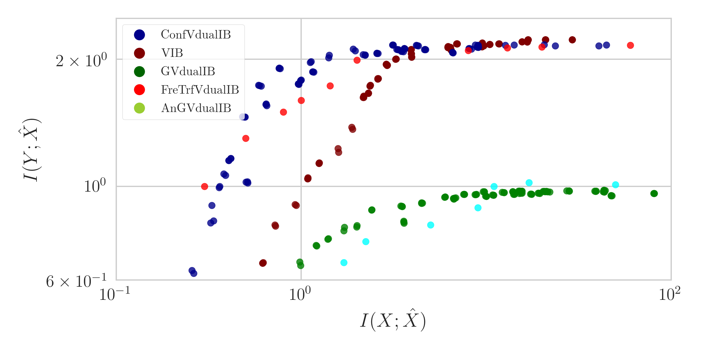
Refer to caption
Figure A2: The information plane for the different noise models.

H.4.1 Training VIB model with noise

In our analysis, we train a VIB model with the same noise model as the VdualIB. Namely, instead of training with a deterministic label (one-hot vector of zeros and ones), we use our noise model also for the VIB. As mentioned in the text, this training procedure is closely related to label smoothing. In FigureΒ A3, we present the loss function of the VIB on CIFAR10 with and without the noise models along the training process for 333 different values of β𝛽\beta. For a small β𝛽\beta (left) both regimes under-fit the data as expected. However, when we enlarge β𝛽\beta, we can see that the labels’ noise makes the training more stable and for a high value of β𝛽\beta (right) training without noise over-fits the data and the loss increases.
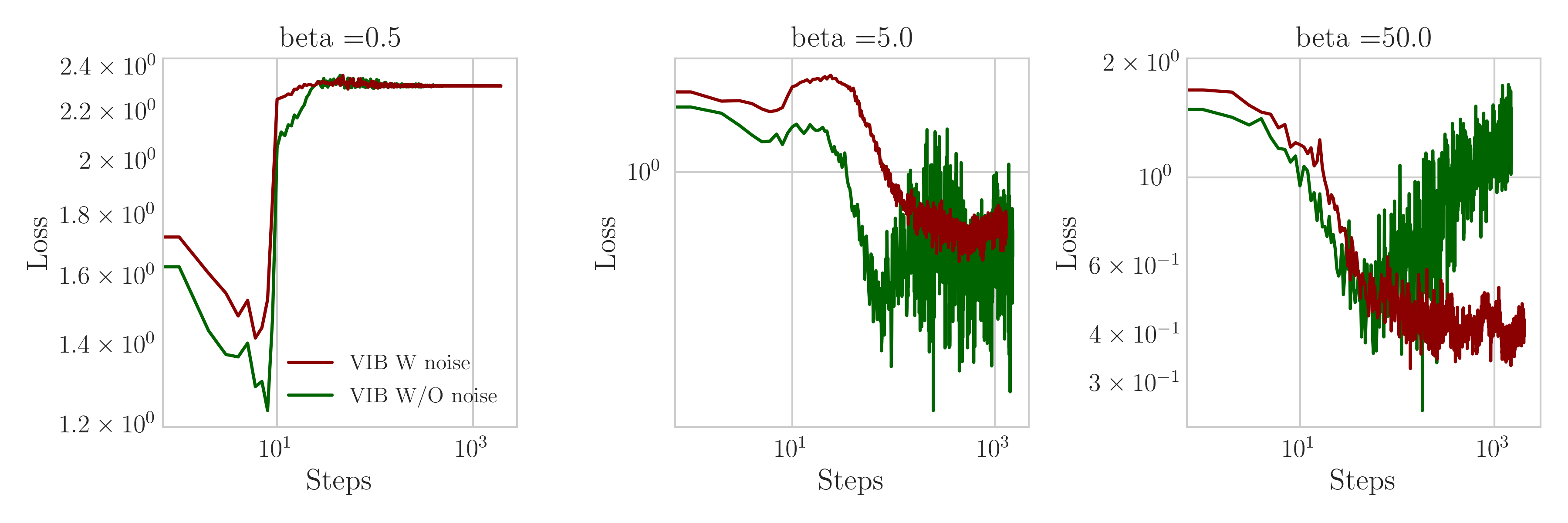
Refer to caption
Figure A3: The influence of a noise model on the VIB performance. Loss as function of the update steps for different values of β𝛽\beta, Ξ²=0.5,5.0.50.0𝛽0.55.0.50.0\beta=0.5,5.0.50.0 from left to right.

The confusion matrix for the CIFAR10 data set is:

(0.8780.0.0170.0130.0020.0010.0820.0.0070.0.0.9840.0020.0090.0010.0.0030.0.0.0.0130.0010.8960.0090.0380.0.0430.0.0.[0.0220.0040.0110.9130.0230.0.0270.0.0010.0.0.0.0720.0220.850.0.0580.0.0.0.0.0.0.0.0.9820.0.0110.0.0070.0990.0010.0490.0210.0550.0.7680.0.0050.0.0.0.0.0.0.0060.0.9760.0.0190.0040.0010.0010.0010.0040.0020.0030.0010.980.0010.0.0.0.0.0.0040.0.020.0010.974)\displaystyle\begin{pmatrix}0.878&0.&0.017&0.013&0.002&0.001&0.082&0.&0.007&0.\\ 0.&0.984&0.002&0.009&0.001&0.&0.003&0.&0.&0.\\ 0.013&0.001&0.896&0.009&0.038&0.&0.043&0.&0.&0.\\ [0.022&0.004&0.011&0.913&0.023&0.&0.027&0.&0.001&0.\\ 0.&0.&0.072&0.022&0.85&0.&0.058&0.&0.&0.\\ 0.&0.&0.&0.&0.&0.982&0.&0.011&0.&0.007\\ 0.099&0.001&0.049&0.021&0.055&0.&0.768&0.&0.005&0.\\ 0.&0.&0.&0.&0.&0.006&0.&0.976&0.&0.019\\ 0.004&0.001&0.001&0.001&0.004&0.002&0.003&0.001&0.98&0.001\\ 0.&0.&0.&0.&0.&0.004&0.&0.02&0.001&0.974\end{pmatrix}

H.5 CIFAR100 results

As mentioned in the text, we trained VdualIB networks also on CIFAR100. For this, we used the same 28βˆ’10281028-10 Wide ResNet with a confusion matrix as our noise model. The confusion matrix was calculated based on the predictions of a deterministic network. The deterministic network achieved 80.2%percent80.280.2\% accuracy on CIFAR100. In 4(a), we can see the information plane for both VdualIB and the VIB models. As we can see, both models are monotonic with I​(X;X^)𝐼𝑋^𝑋I(X;\hat{X}), however the VIB’s performance is better. The VIB achieves higher values of information with the labels along with more compressed representation at any given level of predication. Although a broader analysis is required, and possible further parameter tuning of the architecture, we hypothesize that the caveat is in the noise model used for the VdualIB. Using a noise model which is based on a network that achieves almost 20%percent2020\% error might be insufficient in this case. It might be that β€œerrors” in the noise model becomes similar to random errors, similar to the Gaussian case, and hence depicting similar learning performance to the GVdualIB case.

When we look at the information with the input as a function of time ,FigureΒ 4(b), we see that similar to the FasionMNIST and CIFAR10 results, the information saturates for small values of β𝛽\beta, but over-fits for higher values of it.
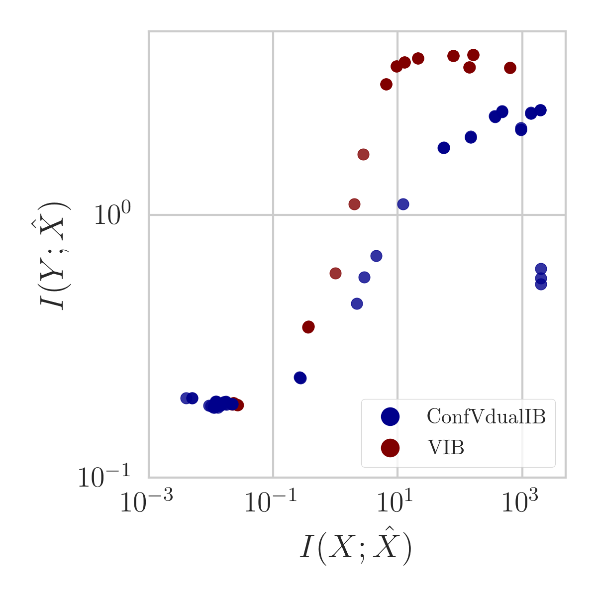
Refer to caption
(a) The information plane
Refer to caption
(b) I​(X;X^)𝐼𝑋^𝑋I(X;\hat{X}) vs. update steps for different b​e​t​aπ‘π‘’π‘‘π‘Žbeta’s
Figure A4: Experiments over CIFAR100. (a)π‘Ž(a) The information plane of the ConfVdualIB and VIB for a range of β𝛽\beta values at the final training step. (b)𝑏(b) The evolution of the the ConfVdualIB’s I​(X;X^)𝐼𝑋^𝑋I(X;\hat{X}) along the optimization update steps.