Hybrid Beamforming for Massive MIMO Over-the-Air Computation

Abstract

Over-the-air computation (AirComp) has been recognized as a promising technique in Internet-of-Things (IoT) networks for fast data aggregation from a large number of wireless devices. However, as the number of devices becomes large, the computational accuracy of AirComp would seriously degrade due to the vanishing signal-to-noise ratio (SNR). To address this issue, we exploit the massive multiple-input multiple-output (MIMO) with hybrid beamforming, in order to enhance the computational accuracy of AirComp in a cost-effective manner. In particular, we consider the scenario with a large number of multi-antenna devices simultaneously sending data to an access point (AP) equipped with massive antennas for functional computation over the air. Under this setup, we jointly optimize the transmit digital beamforming at the wireless devices and the receive hybrid beamforming at the AP, with the objective of minimizing the computational mean-squared error (MSE) subject to the individual transmit power constraints at the wireless devices. To solve the non-convex hybrid beamforming design optimization problem, we propose an alternating-optimization-based approach, in which the transmit digital beamforming and the receive analog and digital beamforming are optimized in an alternating manner. In particular, we propose two computationally efficient algorithms to handle the challenging receive analog beamforming problem, by exploiting the techniques of successive convex approximation (SCA) and block coordinate descent (BCD), respectively. It is shown that for the special case with a fully-digital receiver at the AP, the achieved MSE of the massive MIMO AirComp system is inversely proportional to the number of receive antennas. Furthermore, numerical results show that the proposed hybrid beamforming design substantially enhances the computation MSE performance as compared to other benchmark schemes, while the SCA-based algorithm performs closely to the performance upper bound achieved by the fully-digital beamforming.

I Introduction

Future Internet-of-Things (IoT) networks need to support an enormous number of wireless devices for sensing the environment, aggregate massive sensing data for analysis, and accordingly take physical actions[Agiwal2016, Lin2017]. Conventionally, such data aggregation is implemented via wireless devices individually sending their data to an access point (AP) or a fusion center over wireless multiple access channels, in which the AP may need to decode the individual messages from each device by treating messages from others as harmful interference. Nevertheless, for practical IoT applications, the AP may be interested in computing a certain function value (e.g., the sum value) of the aggregated data rather than the individual messages (e.g., in federated learning setups [Yang2020]). In this case, the above conventional multiple access scheme may not be energy- or spectral-efficient and may also lead to excessively long network latency, especially when the number of devices becomes significantly large. To overcome the drawback, the over-the-air computation (AirComp) technique has been proposed recently, which utilizes the co-channel interference among devices as a beneficial factor for functional computation [Abari2016, ZhuAir1]. By exploiting the signal superposition property of multiple access channels, the AirComp technique is able to directly compute a class of nomographic functions (e.g., arithmetic mean, weighted sum, geometric mean, polynomial, and Euclidean norm) of distributed sensing data from the concurrent transmission of distributed wireless devices [Boche2015].

In general, AirComp can be implemented in both analog and digital modes. While the simple uncoded analog transmission was shown to achieve the minimum functional distortion when the data sources follow the independent and identically distributed (i.i.d.) Gaussian distribution [Gastpar2008], coding was shown to be necessary for improving the computation performance under the bivariate Gaussian [Wagner2008] and correlated Gaussian [Soundararajan2012] distributed data sources. Besides, for analog AirComp, the computation mean-squared error (MSE) is normally adopted as the performance metric. In the single-antenna setup, a proper power control is essential for minimizing the computation MSE [Xiao2008, Wang2011, Cao2019]. For instance, under the coherent multiple access channel, the optimal power control strategy for minimizing the computation MSE was proposed in [Xiao2008] by using convex optimization, and optimal power allocation strategies were proposed in [Wang2011] for minimizing the distortion outage probability (defined as the probability that the computation MSE exceeds a given threshold). Furthermore, under fading channels, the optimal power allocation strategy for minimizing the average computation MSE was studied [Cao2019]. In particular, multi-antenna beamforming is an efficient technique to further enhance the computation MSE performance. For instance, the authors in [ZhuAir1] investigated the multiple-input multiple-output (MIMO) AirComp for computing multiple functions simultaneously, in which a closed-form equalization at the AP was proposed to minimize the computation MSE under the zero-forcing (ZF) transmit beamforming at wireless devices. Notice that the implementation of AirComp requires the synchronization among all devices; towards this end, the so-called AirShare design was developed in [Abari2015], where a shared clock was broadcast to all devices to facilitate synchronization.

On the other hand, digital AirComp was proposed to enhance computational accuracy via proper coding methods [Nazer2007, Zhang2006, Appuswamy2014, Erez2005, Nazer2011, Jeon2016]. The idea of digital AirComp first appeared for functional computation in wireless sensor networks (see, e.g., [Nazer2007]) and physical-layer network coding in a two-way relay channel (see, e.g., [Zhang2006]). For AirComp, the achievable computation rate under different system setups was characterized in [Nazer2011] and [Jeon2016], which is defined as the number of functional values computed per unit time under a predefined computational accuracy. Furthermore, to enable multi-function computation with enhanced computation rate, the authors in [Wu2020] integrated the idea of non-orthogonal multiple access (NOMA) [Dai2015] in AirComp, in which multiple functions from different wireless devices are superposed in each resource block.

In this paper, we particularly focus our study on the analog AirComp, in which wireless devices send uncoded data to a single AP for functional computation. In practice, the implementation of AirComp over large-scale wireless networks faces several technical challenges. For instance, as the number of wireless devices increases, the computation performance in AirComp systems may seriously degrade, due to the vanishing of the received signal-to-noise ratio (SNR) at the AP. As a remedy, massive MIMO [Marzetta2010] is considered as a promising viable solution to improve the computational accuracy of AirComp systems by exploiting its rich spatial degrees of freedom and tremendous array gain. To the best of our knowledge, the exploitation of massive MIMO for AirComp has not been reported in the literature yet. Hence, it motivates us to consider the combination of massive MIMO and AirComp to improve the computation accuracy.

Despite the potential benefits, the amalgamation of massive MIMO and AirComp would incur high fabrication cost and energy consumption due to the conditional large numbers of radio frequency (RF) chains as well as analog-to-digital converters (ADCs) associated with antennas. To address these issues, the hybrid beamforming structure has emerged as a promising solution, which allows the AP to employ a smaller number of RF chains than that of antenna elements [Sudarshan2006, Rial2016, Yang2018, Hur2013, Alkhateeb2014, Han2019, Zhai2017, Yu2016, Dsouza2018, Liu2019, Song2020]. Considering the tradeoff between performance versus complexity, different types of hybrid beamforming (e.g., fully-connected [Hur2013, Alkhateeb2014, Yu2016, Zhai2017, Yang2018, Han2019, Liu2019] and partially-connected [Sudarshan2006, Rial2016, Dsouza2018, Song2020]) with different kinds of RF electronic modules (e.g., analog switches [Sudarshan2006, Rial2016] and analog phase shifters [Hur2013, Alkhateeb2014, Yu2016, Zhai2017, Yang2018, Dsouza2018, Han2019, Liu2019, Song2020]) have been investigated. In particular, the fully-connected hybrid beamforming is appealing as it can achieve better performance with each RF chain connected to all antennas, while the partially-connected hybrid beamforming shows a lower complexity but compromised performance, since it allows every RF chain to connect to only part of antennas.

Although there have been a handful of prior works investigating hybrid beamforming for massive MIMO communication systems [Sudarshan2006, Rial2016, Yang2018, Hur2013, Alkhateeb2014, Han2019, Zhai2017, Yu2016, Dsouza2018, Liu2019, Song2020], these designs cannot be directly applied to massive MIMO AirComp systems, due to the following reasons. First, the design objectives are fundamentally different. In massive MIMO communication systems, the hybrid beamforming design aims to maximize the communication rate by eliminating the interference, while in massive MIMO AirComp systems, the hybrid beamforming design targets for minimizing the computation error by harnessing the “interference”. Second, inspired by the low-latency requirement of data-intensive IoT applications, the hybrid beamforming in massive MIMO AirComp systems should achieve good computational accuracy with a less computational complexity/latency. Motivated by the above observations, in this paper, we investigate the hybrid beamforming design for massive MIMO AirComp systems. As an initial attempt, we adopt the fully-connected hybrid beamforming with analog phase shifters to achieve full spatial degrees of freedom of massive MIMO for AirComp.

The main results of this paper are summarized as follows.

• We consider a massive MIMO AirComp system with a massive-antenna AP and a massive number of wireless devices, which aims to compute multiple arithmetic sum functions of the recorded signals from all the devices. Our objective is to jointly optimize the transmit digital beamforming, the receive analog beamforming, and the receive digital beamforming to minimize the computation MSE. The formulated problem is generally intractable due to the highly coupled variables in the objective function and the constant modulus constraints for the receive analog beamforming.

• To address the non-convex hybrid beamforming optimization problem, we propose an alternating-optimization-based approach to alternately optimize the transmit beamforming and the receive analog and digital beamforming. In particular, we optimize the receive analog beamforming by applying two methods, namely the successive convex approximation (SCA) and block coordinate descent (BCD), respectively. While the SCA-based method leads to a better performance, the BCD-based method enjoys a lower computational complexity at the expense of a compromised performance.

• To gain more insights, we analyze the MSE performance for a special case with a fully-digital receiver at the AP. In this case, we show that the optimal (digital) receive beamforming follows the sum-minimization-MSE (sum-MMSE) structure. With the help of the sum-MMSE receive beamforming, we prove that the computation MSE is inversely proportional to the number of receive antennas when the AP adopts the techniques of massive MIMO.

• Furthermore, numerical results show that the proposed hybrid beamforming design substantially improves the computation MSE performance of multi-function/multi-modal massive MIMO AirComp systems as compared to other benchmark scheme inspired by the ZF-based fully-digital beamforming design in [ZhuAir1]. The SCA-based algorithm is shown to perform closely to the performance upper bound achieved by the fully-digital beamforming.

The remainder of this paper is organized as follows. Section II introduces the system model and formulates the computational MSE minimization problem. Section III presents the alternating-optimization-based approaches to address the formulated problem, where two algorithms are proposed to optimize the receive analog beamforming based on SCA and BCD, respectively. Section IV analyzes the MSE performance for the special case with fully-digital beamforming design. Section V presents the numerical results. Finally, Section VI draws the conclusion.

Notations: Throughout this paper, we adopt bold upper-case letters for matrices and bold lower-case letters for vectors. For a matrix $\mathbf{A}$, $\mathbf{A}(i,j)$ represents the entry on the $i^{th}$ row and the $j^{th}$ column, while $\mathbf{A}^{\dagger}$, $\mathbf{A}^{*}$, $\mathbf{A}^{T}$, and $\mathbf{A}^{H}$ denote its Moore-Penrose pseudo inverse, conjugate, transpose, and Hermitian transpose, respectively. Furthermore, $\mathbf{I}$ denotes the identity matrix whose dimension will be clear from the context, and $\mathbb{C}^{m\times n}$ denotes the $m$-by-$n$ dimensional complex space. The notations $\mathbb{E}(\cdot)$, ${\rm Tr}(\cdot)$, $\det(\cdot)$, $\text{vec}(\cdot)$, $\mathbb{R}(\cdot)$, and $\|\cdot\|$ represent the expectation, trace, determinant, vectorization, real part, and Frobenius norm of an input variable, respectively. $\bigtriangledown_{\bm{x}}f(\bm{x})$ denotes the gradient of $f(\bm{x})$ with respect to $\bm{x}$. $\circ$ is the Hadamard product between two matrices. The circularly symmetric complex Gaussian (CSCG) distribution with mean $\bm{\Upsilon}$ and covariance matrix $\bm{\Phi}$ is denoted by $\mathcal{CN}(\bm{\Upsilon},\bm{\Phi})$. $\text{mod}(a,b)$ is the modulus operation of $a$ with respect to $b$.

II System Model And Problem Formulation

II-A System Model

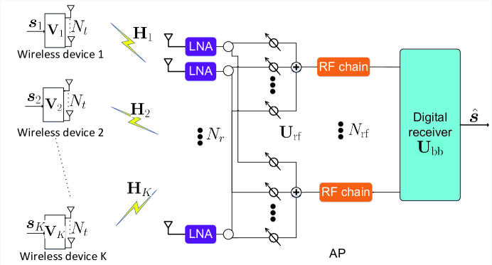
Figure 1: A massive MIMO AirComp system with hybrid beamforming.

We consider a massive MIMO AirComp system as shown in Fig. 1, where the AP simultaneously serves $K$ wireless devices. Suppose each device is equipped with $N_{t}$ transmit antennas and the AP is equipped with $N_{r}$ receive antenna elements, each of which is connected to a low-noise amplifier (LNA). With massive MIMO, it is assumed that $N_{r}\gg N_{t}$. Besides, fully-digital beamforming is adopted at the wireless devices while hybrid beamforming with only $N_{\mathrm{rf}}$ RF chains is implemented at the AP, with $N_{\mathrm{rf}}\leq N_{r}$, to reduce the hardware cost and implementation complexity [Zhai2017, Yu2016]. For the purpose of initial investigation, we consider the fully-connected hybrid beamforming with phase shifters to achieve full spatial degrees of freedom of massive MIMO. For the convenience of expression, we denote $\mathcal{N}_{r}\triangleq\{1,2,\ldots,N_{r}\}$ and $\mathcal{N}_{\mathrm{rf}}\triangleq\{1,2,\ldots,N_{\mathrm{rf}}\}$ as the antenna and RF chain sets, respectively.

In this massive MIMO AirComp system, every device records $L$ heterogeneous time-varying parameters (e.g., humidity, temperature, noise) of the environment with $L\leq\min(N_{\mathrm{rf}},N_{t})$. In particular, since we focus on studying multi-function/multi-modal massive MIMO AirComp systems, we have $L>1$. The devices simultaneously transmit the recorded data to the AP for computation. At a particular time slot, we denote $s_{kl}$ as the recorded data of the $l$th parameter at device $k$, $k\in\mathcal{K}\triangleq\{1,2,\ldots,K\},l\in\mathcal{L}\triangleq\{1,2,\ldots,L\}$, and $\bm{s}_{k}=[s_{k1},\cdots,s_{KL}]^{T}\in\mathbb{C}^{L\times 1}$ as the composite record vector at that device. Without loss of generality, the collected data vector is assumed to be normalized and independent form each other, i.e., $\mathbb{E}(\bm{s}_{k}\bm{s}_{k}^{H})=\mathbf{I},\mathbb{E}(\bm{s}_{k}\bm{s}_{j}^{H})=\bm{0},\forall k,j\in\mathcal{K},k\neq j$, where the normalization factor for each data type is uniform for all devices and can be inverted at the AP for recovering the original data.

In order to support ultrafast data computation, the AP exploits the superposition property of the multiple access channel to directly compute the target nomographic function with reduced communication overheads. In this paper, we are interested in the sum operation, while the design is also extendable for other nomographic functions [Boche2015]. Towards this end, each device transmits a vector $\bm{s}_{k}$ and the AP is interested in estimating $\bm{s}=\sum\limits_{k=1}^{K}\bm{s}_{k}$, which is referred to as the target-function vector [ZhuAir1].

Referring to the proposed system model, the transmitted signal by device $k$ is denoted by

$$\bm{x}_{k}=\mathbf{V}_{k}\bm{s}_{k},$$ (1)

where $\mathbf{V}_{k}\in\mathbb{C}^{N_{t}\times L}$ denotes the transmit beamforming matrix. Let $P$ denote the maximum transmit power at each device. Accordingly, we have $\mathbb{E}(\|\bm{x}_{k}\|^{2})={\rm Tr}(\mathbf{V}_{k}\mathbf{V}_{k}^{H})\leq P,\forall k\in\mathcal{K}$.

It is assumed that the channel state information (CSI) is perfectly known at both the AP and the devices. Then the received signal vector at the AP is given by

$$\bm{y}=\sum\limits_{k=1}^{K}\mathbf{H}_{k}\mathbf{V}_{k}\bm{s}_{k}+\bm{n},$$ (2)

where $\mathbf{H}_{k}\in\mathbb{C}^{N_{r}\times N_{t}}$ denotes the channel matrix from device $k$ to the AP and $\bm{n}\in\mathbb{C}^{N_{r}\times 1}$ is the AWGN vector with $\bm{n}\sim\mathcal{CN}(\mathbf{0},\sigma^{2}\mathbf{I})$.

Next, the AP adopts the hybrid beamforming for AirComp. Here, the hybrid beamforming needs to be properly designed for not only harnessing part of the inter-device interference to facilitate the computation, but also eliminating the inter-function interference. Let $\mathbf{U}_{\mathrm{rf}}\in\mathbb{C}^{N_{r}\times N_{\mathrm{rf}}}$ denote the receive analog beamforming, whose entries have constant modulus, i.e., $|\mathbf{U}_{\mathrm{rf}}(i,j)|=1$, $\forall i\in\mathcal{N}_{r}$, $j\in\mathcal{N}_{\mathrm{rf}}$, and $\mathbf{U}_{\mathrm{bb}}\in\mathbb{C}^{N_{\mathrm{rf}}\times L}$ denote the low-dimension receive digital beamforming. Therefore, the processed signal after the adopted hybrid beamforming can be expressed as

$$\hat{\mathbf{s}}=\mathbf{U}_{\mathrm{bb}}^{H}\mathbf{U}_{\mathrm{rf}}^{H}\bm{y}.$$ (3)

Consequently, the computational accuracy is measured by the MSE between $\hat{\bm{s}}$ and $\bm{s}$, which is given by [ZhuAir1]

$$\begin{split}&\text{MSE}(\{\mathbf{V}_{k}\},\mathbf{U}_{\mathrm{rf}},\mathbf{U}_{\mathrm{bb}})\\ &=\mathbb{E}[\|\bm{s}-\hat{\bm{s}}\|^{2}]\\ &=\sum\limits_{k=1}^{K}{\rm Tr}\left[(\mathbf{U}_{\mathrm{bb}}^{H}\mathbf{U}_{\mathrm{rf}}^{H}\mathbf{H}_{k}\mathbf{V}_{k}-\mathbf{I})(\mathbf{U}_{\mathrm{bb}}^{H}\mathbf{U}_{\mathrm{rf}}^{H}\mathbf{H}_{k}\mathbf{V}_{k}-\mathbf{I})^{H}\right]+\sigma^{2}{\rm Tr}(\mathbf{U}_{\mathrm{bb}}^{H}\mathbf{U}_{\mathrm{rf}}^{H}\mathbf{U}_{\mathrm{rf}}\mathbf{U}_{\mathrm{bb}}).\end{split}$$ (4)

II-B Problem Formulation

In this work, we are interested in minimizing the MSE defined in (4) by jointly optimizing the transmit beamforming $\{\mathbf{V}_{k}\}$ at the devices and the receive hybrid beamforming $\mathbf{U}_{\mathrm{rf}}$ and $\mathbf{U}_{\mathrm{bb}}$ at the AP, subject to the constant modulus constraints on $\mathbf{U}_{\mathrm{rf}}$ and the maximum power budget constraints on $\{\mathbf{V}_{k}\}$. In particular, the MSE minimization problem can be formulated as

$$\begin{split}\mathcal{P}1\!:\;&\mathop{\mathrm{minimize}}\limits_{\mathbf{V}_{k},\mathbf{U}_{\mathrm{rf}},\mathbf{U}_{\mathrm{bb}}}~{}\text{MSE}(\{\mathbf{V}_{k}\},\mathbf{U}_{\mathrm{rf}},\mathbf{U}_{\mathrm{bb}})\\ &\text{subject to}~{}~{}{\rm Tr}(\mathbf{V}_{k}\mathbf{V}_{k}^{H})\leq P,\forall k\in\mathcal{K}\\ &~{}~{}~{}~{}~{}~{}~{}~{}~{}~{}~{}~{}~{}~{}|\mathbf{U}_{\mathrm{rf}}(i,j)|=1,\forall i\in\mathcal{N}_{r},j\in\mathcal{N}_{\mathrm{rf}}.\end{split}$$ (5)

Problem $\mathcal{P}1$ is difficult to solve, as the optimization variables $\{\mathbf{V}_{k}\}$, $\mathbf{U}_{\mathrm{rf}}$, and $\mathbf{U}_{\mathrm{bb}}$ are highly coupled in the objective function while the unit modulus constraints of $\mathbf{U}_{\mathrm{rf}}$ are highly non-convex. Furthermore, problem $\mathcal{P}1$ aims to minimize the computation MSE for recovering $\bm{s}=\sum\limits_{k=1}^{K}\bm{s}_{k}$ by exploiting the interference from various wireless devices. Note that this is significantly different from the conventional hybrid beamforming design problems in massive MIMO systems which mainly maximize the communication rate (for decoding $\bm{s}_{k}$’s individually) by eliminating the inter-device interference. Hence, the conventional designs are not directly applicable to the considered problem $\mathcal{P}1$. Besides, due to the requirement of ultrafast computation for data aggregation, attaining an efficient solution to problem $\mathcal{P}1$ with low computational complexity is also desirable. To the best of our knowledge, however, there lacks computationally efficient and systematic algorithms to solve such non-convex problems optimally. As a compromise approach, in the next section, by exploiting the structure of problem, we propose an alternating-optimization-based method to iteratively optimize $\{\mathbf{V}_{k}\}$, $\mathbf{U}_{\mathrm{rf}}$, and $\mathbf{U}_{\mathrm{bb}}$.

III Hybrid Beamforming Designs

In this section, a novel hybrid beamforming approach is proposed to handle problem $\mathcal{P}1$, by updating $\{\mathbf{V}_{k}\}$, $\mathbf{U}_{\mathrm{rf}}$, and $\mathbf{U}_{\mathrm{bb}}$ in an alternating manner. In the following, we first optimize the transmit beamforming $\{\mathbf{V}_{k}\}$ by using the Lagrange duality method, then we update the receive analog beamforming $\mathbf{U}_{\mathrm{rf}}$ by using the techniques of SCA or BCD, and finally optimize $\mathbf{U}_{\mathrm{bb}}$ by exploiting the first order optimality condition.

III-A Optimization of Transmit Beamforming $\{\mathbf{V}_{k}\}$

First, we focus on the optimization of $\{\mathbf{V}_{k}\}$ under given $\mathbf{U}_{\mathrm{rf}}$ and $\mathbf{U}_{\mathrm{bb}}$. In this case, problem $\mathcal{P}1$ can be equivalently decomposed into the following $K$ subproblems each for one device $k\in\mathcal{K}$, by ignoring the constant term $\sigma^{2}{\rm Tr}(\mathbf{U}_{\mathrm{rf}}\mathbf{U}_{\mathrm{bb}}\mathbf{U}_{\mathrm{bb}}^{H}\mathbf{U}_{\mathrm{rf}}^{H})$:

$$\begin{split}\mathcal{P}2\!:\;&\mathop{\mathrm{minimize}}\limits_{\mathbf{V}_{k}}{\rm Tr}\left[(\mathbf{U}_{\mathrm{bb}}^{H}\mathbf{U}_{\mathrm{rf}}^{H}\mathbf{H}_{k}\mathbf{V}_{k}-\mathbf{I})(\mathbf{U}_{\mathrm{bb}}^{H}\mathbf{U}_{\mathrm{rf}}^{H}\mathbf{H}_{k}\mathbf{V}_{k}-\mathbf{I})^{H}\right]\\ &\text{subject to}~{}{\rm Tr}(\mathbf{V}_{k}\mathbf{V}_{k}^{H})\leq P,\forall k\in\mathcal{K}.\end{split}$$ (6)

Problem $\mathcal{P}2$ is a convex quadratic optimization problem that satisfies the Slater’s constraint condition, and therefore, this problem can be optimally solved by using standard convex optimization techniques [Boyd2004]. To gain more insights, we apply the Lagrange duality method to find a semi-closed-form optimal solution, which is summarized in the following lemma.

Lemma 1

The optimal transmit beamforming solution to problem $\mathcal{P}2$ for device $k$ is given by:

$$\mathbf{V}_{k}^{\mathrm{opt}}=(\mathbf{H}_{k}^{H}\mathbf{U}_{\mathrm{rf}}\mathbf{U}_{\mathrm{bb}}\mathbf{U}_{\mathrm{bb}}^{H}\mathbf{U}_{\mathrm{rf}}^{H}\mathbf{H}_{k}+\mu_{k}^{\mathrm{opt}}\mathbf{I})^{-1}\mathbf{H}_{k}^{H}\mathbf{U}_{\mathrm{rf}}\mathbf{U}_{\mathrm{bb}},$$ (7)

where $\mu_{k}^{\mathrm{opt}}\geq 0,k\in\mathcal{K},$ denotes the optimal Lagrange multiplier associated with the power constraint for device $k$ in problem $\mathcal{P}2$. Here, if $\mathbf{H}_{k}^{H}\mathbf{U}_{\mathrm{rf}}\mathbf{U}_{\mathrm{bb}}\mathbf{U}_{\mathrm{bb}}^{H}\mathbf{U}_{\mathrm{rf}}^{H}\mathbf{H}_{k}$ is invertible and

$${\rm Tr}((\mathbf{H}_{k}^{H}\mathbf{U}_{\mathrm{rf}}\mathbf{U}_{\mathrm{bb}}\mathbf{U}_{\mathrm{bb}}^{H}\mathbf{U}_{\mathrm{rf}}^{H}\mathbf{H}_{k})^{-2}\mathbf{H}_{k}^{H}\mathbf{U}_{\mathrm{rf}}\mathbf{U}_{\mathrm{bb}}\mathbf{U}_{\mathrm{bb}}^{H}\mathbf{U}_{\mathrm{rf}}^{H}\mathbf{H}_{k})<P$$ (8)

holds, we have $\mu_{k}^{\mathrm{opt}}=0$; otherwise, $\mu_{k}^{\mathrm{opt}}$ is chosen such that the equality in (9) holds.

$${\rm Tr}((\mathbf{H}_{k}^{H}\mathbf{U}_{\mathrm{rf}}\mathbf{U}_{\mathrm{bb}}\mathbf{U}_{\mathrm{bb}}^{H}\mathbf{U}_{\mathrm{rf}}^{H}\mathbf{H}_{k}+\mu_{k}^{\mathrm{opt}}\mathbf{I})^{-2}\mathbf{H}_{k}^{H}\mathbf{U}_{\mathrm{rf}}\mathbf{U}_{\mathrm{bb}}\mathbf{U}_{\mathrm{bb}}^{H}\mathbf{U}_{\mathrm{rf}}^{H}\mathbf{H}_{k})=P.$$ (9)

Proof:

See Appendix A. ∎

From Lemma 1, we can see that $\{\mathbf{V}_{k}\}$ is optimized by considering the following two cases. If the transmit power budget $P$ is sufficiently large, then we choose $\mu_{k}^{\mathrm{opt}}=0$ such that the objective function value of problem $\mathcal{P}2$ is forced to be zero; otherwise, if the transmit power budget $P$ is limited, then we choose $\mu_{k}^{\mathrm{opt}}$ such that the transmit power is fully used to minimize the computation MSE.

III-B Optimization of Receive Analog Beamforming $\mathbf{U}_{\mathrm{rf}}$

In this subsection, we optimize $\mathbf{U}_{\mathrm{rf}}$ under given $\{\mathbf{V}_{k}\}$ and $\mathbf{U}_{\mathrm{bb}}$, for which the problem is given by

$$\begin{split}\mathcal{P}3\!:\;&\mathop{\mathrm{minimize}}\limits_{\mathbf{U}_{\mathrm{rf}}}\text{MSE}(\{\mathbf{V}_{k}\},\mathbf{U}_{\mathrm{rf}},\mathbf{U}_{\mathrm{bb}})\\ &\text{subject to}~{}~{}|\mathbf{U}_{\mathrm{rf}}(i,j)|=1,\forall i\in\mathcal{N}_{r},j\in\mathcal{N}_{\mathrm{rf}}.\end{split}$$ (10)

Problem $\mathcal{P}3$ is still challenging to solve mainly due to the constant modulus constraints which are intrinsically non-convex. To address this issue, we propose two algorithms by using SCA and BCD, respectively.

III-B1 SCA

To gain more insights, motivated by [Liu2019], we transform problem $\mathcal{P}3$ into a more tractable form by exploiting the SCA method. To start with, we first rewrite the constant modulus constraints in its exponential form. Let $\bm{u}_{\mathrm{rf}}=\text{vec}(\mathbf{U}_{\mathrm{rf}})\in\mathbb{C}^{N_{r}N_{\mathrm{rf}}\times 1}$ and $\bm{\theta}\triangleq[\theta_{1},\theta_{2},\ldots,\theta_{N_{r}N_{\mathrm{rf}}}]^{T}$ denote the vectorization of $\mathbf{U}_{\mathrm{rf}}$ and the corresponding phase vector of $\bm{u}_{\mathrm{rf}}$, respectively. Then problem $\mathcal{P}3$ is transformed to the following equivalent problem:

$$\begin{split}\mathcal{P}4\!:\;&\mathop{\mathrm{minimize}}\limits_{\bm{\theta}}f(\bm{\theta})\\ &\text{subject to}~{}~{}-\pi\leq\bm{\theta}(i)\leq\pi,\forall i\in\mathcal{Y},\end{split}$$ (11)

where

$$f(\bm{\theta})=\text{MSE}(\{\mathbf{V}_{k}\},\mathbf{U}_{\mathrm{rf}}(\bm{\theta}),\mathbf{U}_{\mathrm{bb}}),$$ (12)

$$\mathcal{Y}\triangleq\{1,2,\ldots,N_{r}N_{\mathrm{rf}}\}.$$ (13)

Note that $\mathbf{U}_{\mathrm{rf}}(\bm{\theta})$ in (12) means that $\mathbf{U}_{\mathrm{rf}}$ is a function of $\bm{\theta}$, which can be written element-wisely as:

$$\mathbf{U}_{\mathrm{rf}}(i,j)=e^{\sqrt{-1}\bm{\theta}((j-1)N_{r}+i)},\forall i\in\mathcal{N}_{r},j\in\mathcal{N}_{\mathrm{rf}},$$ (14)

where $\sqrt{-1}$ denotes the imaginary unit.

With the above derivation, we transform the intractable constant modulus constraints into linear constraints equivalently. From problem $\mathcal{P}4$, we can see that the objective function is non-convex. To address this issue, according to the technique of SCA, we need to find a surrogate function of $f(\bm{\theta})$ first. Let $r$ and $\bm{\theta}_{r}$ denote the iteration number and the current point in the $r$th iteration. Under the given local point $\bm{\theta}_{r}$, we can obtain one of the corresponding surrogate functions denoted by $\hat{f}(\bm{\theta},\bm{\theta}_{r})$ via exploiting the first-order Taylor approximation, which is given by

$$\hat{f}(\bm{\theta},\bm{\theta}_{r})=f(\bm{\theta}_{r})+\bm{\gamma}^{H}_{\bm{\theta}_{r}}(\bm{\theta}-\bm{\theta}_{r})+\tau\|\bm{\theta}-\bm{\theta}_{r}\|^{2},$$ (15)

$$\bm{\gamma}_{\bm{\theta}_{r}}=\bigtriangledown_{\bm{\theta}}f(\bm{\theta})|_{\bm{\theta}=\bm{\theta}_{r}}=-\text{vec}\{2\mathbb{R}[\sqrt{-1}\mathbf{U}_{\mathrm{rf},r}^{*}\circ\mathbf{F}_{r}]\},$$ (16)

$$\mathbf{F}_{r}=\left(\sum\limits_{k=1}^{K}\mathbf{H}_{k}\mathbf{V}_{k}\mathbf{V}_{k}^{H}\mathbf{H}_{k}^{H}+\sigma^{2}\mathbf{I}\right)\mathbf{U}_{\mathrm{rf},r}\mathbf{U}_{\mathrm{bb}}\mathbf{U}_{\mathrm{bb}}^{H}-\sum\limits_{k=1}^{K}\mathbf{H}_{k}\mathbf{V}_{k}\mathbf{U}_{\mathrm{bb}}^{H},$$ (17)

$$\mathbf{U}_{\mathrm{rf},r}(i,j)=e^{\sqrt{-1}\bm{\theta}_{r}((j-1)N_{r}+i)},\forall i\in\mathcal{N}_{r},j\in\mathcal{N}_{\mathrm{rf}}.$$ (18)

Note that the third term in (15) is a proximal regularization term with $\tau>0$ being a small positive number to guarantee the strong convexity and to control the convergence rate [Liu2019]. $\bm{\gamma}_{\bm{\theta}_{r}}$ is the gradient of $f(\bm{\theta})$ with respect to $\bm{\theta}$ at point $\bm{\theta}_{r}$, which is calculated by the chain rule. With the above derivation, we can see that $\hat{f}(\bm{\theta},\bm{\theta}_{r})$ is the upper bound of $f(\bm{\theta}_{r})$. Besides, $\hat{f}(\bm{\theta},\bm{\theta}_{r})$ and $f(\bm{\theta}_{r})$ have the same values and gradient at point $\bm{\theta}_{r}$. Thus, $\hat{f}(\bm{\theta},\bm{\theta}_{r})$ is a valid surrogate function at point $\bm{\theta}_{r}$ [Boyd2004] and the issue of non-convexity of $f(\bm{\theta})$ is addressed.

According to the procedure of SCA, we can update $\bm{\theta}$ and $\mathbf{U}_{\mathrm{rf}}$ by solving the following approximated problem of $\mathcal{P}4$:

$$\begin{split}\mathcal{P}5\!:\;&\mathop{\mathrm{minimize}}\limits_{\bm{\theta}}\hat{f}(\bm{\theta},\bm{\theta}_{r})\\ &\text{subject to}~{}~{}-\pi\leq\bm{\theta}(i)\leq\pi,\forall i\in\mathcal{Y}.\end{split}$$ (19)

Since problem $\mathcal{P}5$ is convex with respect to $\bm{\theta}$, we can optimize $\bm{\theta}$ by checking the first-order optimality condition, for which the optimal solution is given by

$$\bm{\theta}_{r+1}(i)=\text{mod}\left(\bm{\theta}_{r}(i)-\frac{\bm{\gamma}_{\bm{\theta}_{r}}(i)}{2\tau},2\pi\right),\forall i\in\mathcal{Y}.$$ (20)

Finally, the updated variable $\mathbf{U}_{\mathrm{rf},r+1}$ can be obtained by

$$\mathbf{U}_{\mathrm{rf},r+1}(i,j)=e^{\sqrt{-1}\bm{\theta}_{r+1}((j-1)N_{r}+i)},\forall i\in\mathcal{N}_{r},j\in\mathcal{N}_{\mathrm{rf}}.$$ (21)

The SCA-based algorithm to address problem $\mathcal{P}3$ is summarized in Algorithm 1. According to the analysis in [Liu2019] and [Razaviyayn2013], the proposed SCA-based algorithm can guarantee the convergence of a local optimum theoretically when $\tau$ is chosen properly. However, since the surrogate function is chosen based on the Taylor expansion which does not fully exploit the special structure of problem $\mathcal{P}3$. Hence, it may lead to high computational complexity and slow convergence rate. In the following, we propose an alternative effective approach with lower complexity in handling (10).

Algorithm 1 The SCA-based Algorithm for Solving Problem $\mathcal{P}3$

Set $r=0$, $\tau>0$, and $\epsilon>0$

Repeat

Step 1: Calculate $\bm{\gamma}_{\bm{\theta}_{r}}$ according to (16), (17), and (18);

Step 2: Updata $\bm{\theta}_{r+1}$ according to (20);

Step 3: Update $\mathbf{U}_{\mathrm{rf},r+1}$ according to (21);

Step 4: $r=r+1$;

until the decrease of the objective function in problem $\mathcal{P}3$ is less than $\epsilon$.

III-B2 Low-complexity Design via BCD

Considering the tradeoff between the performance and complexity, we develop an alternative low-complexity algorithm to address problem $\mathcal{P}3$ by exploiting BCD. Based on further manipulation, problem $\mathcal{P}3$ can be equivalently converted as:

$$\begin{split}\mathcal{P}6\!:\;&\mathop{\mathrm{minimize}}\limits_{\mathbf{U}_{\mathrm{rf}}}{\rm Tr}(\mathbf{U}_{\mathrm{rf}}^{H}\mathbf{A}\mathbf{U}_{\mathrm{rf}}\mathbf{C})-2\mathbb{R}\{{\rm Tr}(\mathbf{U}_{\mathrm{rf}}^{H}\mathbf{B})\}\\ &\text{subject to}~{}~{}|\mathbf{U}_{\mathrm{rf}}(i,j)|=1,\forall i\in\mathcal{N}_{r},j\in\mathcal{N}_{\mathrm{rf}},\end{split}$$ (22)

where $\mathbf{A}\triangleq\sum\limits_{k=1}^{K}\mathbf{H}_{k}\mathbf{V}_{k}\mathbf{V}_{k}^{H}\mathbf{H}_{k}^{H}+\sigma^{2}\mathbf{I}$, $\mathbf{B}\triangleq\sum\limits_{k=1}^{K}\mathbf{H}_{k}\mathbf{V}_{k}\mathbf{U}_{\mathrm{bb}}^{H}$, and $\mathbf{C}\triangleq\mathbf{U}_{\mathrm{bb}}\mathbf{U}_{\mathrm{bb}}^{H}$. Since the unit modulus constraints are separable, inspired by [ShiM2018], we can update $\mathbf{U}_{\mathrm{rf}}$ by applying the BCD type algorithm, i.e., in each step we only update one entry of $\mathbf{U}_{\mathrm{rf}}$ by fixing others. Without loss of generality, by defining

$$\phi(\mathbf{U}_{\mathrm{rf}})={\rm Tr}(\mathbf{U}_{\mathrm{rf}}^{H}\mathbf{A}\mathbf{U}_{\mathrm{rf}}\mathbf{C})-2\mathbb{R}\{{\rm Tr}(\mathbf{U}_{\mathrm{rf}}^{H}\mathbf{B})\},$$ (23)

we investigate the problem of minimizing $\phi(\mathbf{U}_{\mathrm{rf}})$ with respect to $\mathbf{U}_{\mathrm{rf}}(i,j)$ for a particular $i\in\mathcal{N}_{r}$ and $j\in\mathcal{N}_{\mathrm{rf}}$ subject to the unit modulus constraint $|\mathbf{U}_{\mathrm{rf}}(i,j)|=1$, i.e.,

$$\mathcal{P}7\!:\;\mathop{\mathrm{minimize}}\limits_{|\mathbf{U}_{\mathrm{rf}}(i,j)|=1}~{}\phi(\mathbf{U}_{\mathrm{rf}}).$$ (24)

It can be observed that the objective function $\phi(\mathbf{U}_{\mathrm{rf}})$ can be re-expressed as a quadratic function with respect to $\mathbf{U}_{\mathrm{rf}}(i,j)$, i.e., $\tilde{\phi}(\mathbf{U}_{\mathrm{rf}}(i,j))\triangleq a|\mathbf{U}_{\mathrm{rf}}(i,j)|^{2}-2\mathbb{R}\{b^{*}\cdot\mathbf{U}_{\mathrm{rf}}(i,j)\}$ for some real number $a$ and some complex number $b$ that will be explained later. Due to the unit modulus constraint, the first term of $\tilde{\phi}(\mathbf{U}_{\mathrm{rf}}(i,j))$ is a constant. Then problem $\mathcal{P}7$ can be simplified as

$$\mathcal{P}8\!:\;\mathop{\mathrm{maximize}}\limits_{|\mathbf{U}_{\mathrm{rf}}(i,j)|=1}~{}\mathbb{R}\{b^{*}\cdot\mathbf{U}_{\mathrm{rf}}(i,j)\}.$$ (25)

It is clear that the optimal solution of $\mathbf{U}_{\mathrm{rf}}(i,j)$ to problem $\mathcal{P}8$ is equal to $\frac{b}{|b|}$. Hence, we only need to obtain $b$ for the update of $\mathbf{U}_{\mathrm{rf}}(i,j)$.

Now we propose a handy method to update the complex number $b$. First, the following equality holds [Petersen2012]:

$$\left.\bigtriangledown_{\mathbf{U}_{\mathrm{rf}}^{*}(i,j)}\tilde{\phi}(\mathbf{U}_{\mathrm{rf}}(i,j))\right|_{\mathbf{U}_{\mathrm{rf}}(i,j)=\tilde{\mathbf{U}}_{\mathrm{rf}}(i,j)}=\frac{1}{2}\left(a\tilde{\mathbf{U}}_{\mathrm{rf}}(i,j)-b\right).$$ (26)

Besides, we have [Petersen2012]

$$\left.\bigtriangledown_{\mathbf{U}_{\mathrm{rf}}^{*}}\tilde{\phi}(\mathbf{U}_{\mathrm{rf}})\right|_{\mathbf{U}_{\mathrm{rf}}=\tilde{\mathbf{U}}_{\mathrm{rf}}}=\frac{1}{2}\left(\mathbf{A}\tilde{\mathbf{U}}_{\mathrm{rf}}\mathbf{C}-\mathbf{B}\right).$$ (27)

Combining (26) and (27), we have $[\mathbf{A}\tilde{\mathbf{U}}_{\mathrm{rf}}\mathbf{C}-\mathbf{B}]_{ij}=a\tilde{\mathbf{U}}_{\mathrm{rf}}(i,j)-b$. By expanding $[\mathbf{A}\tilde{\mathbf{U}}_{\mathrm{rf}}\mathbf{C}]_{ij}$ and checking the coefficient of $\tilde{\mathbf{U}}_{\mathrm{rf}}(i,j)$, we have

$$a\tilde{\mathbf{U}}_{\mathrm{rf}}(i,j)=\mathbf{A}(i,i)\tilde{\mathbf{U}}_{\mathrm{rf}}(i,j)\mathbf{C}(j,j).$$ (28)

Hence, $b$ can be updated according to the following equation:

$$b=\mathbf{A}(i,i)\tilde{\mathbf{U}}_{\mathrm{rf}}(i,j)\mathbf{C}(j,j)-[\mathbf{A}\tilde{\mathbf{U}}_{\mathrm{rf}}\mathbf{C}]_{ij}+\mathbf{B}(i,j).$$ (29)

Considering the above analysis, we can update the entries of $\mathbf{U}_{\mathrm{rf}}$ iteratively. The corresponding algorithm for solving problem $\mathcal{P}6$ is summarized in Algorithm 2, where we need to accordingly update $\mathbf{Q}$ in Step 3 once $\mathbf{U}_{\mathrm{rf}}(i,j)$ is updated (which is done in Step 4). As we can see, Step 3 is the most costly step requiring complexity $\mathcal{O}(N_{r}N_{\mathrm{rf}})$. Hence, it can be shown that the algorithm has complexity of $\mathcal{O}(N_{r}^{2}N_{\mathrm{rf}}^{2})$.

From the above derivation, it is shown that we can obtain the optimal solution of each subproblem for one element of the receive analog beamforming while fixing the others. Considering the concept of the BCD algorithm [Bertsekas2016], the proposed algorithm in Algorithm 2 can converge to a stationary point of problem $\mathcal{P}6$. Furthermore, as compared with the SCA-based algorithm, this element-wise update in the BCD method can reduce the computational complexity by exploiting the special structures of the constant modulus constraints at the expense of certain performance degradation, which will be discussed in Section III-D.

Algorithm 2 BCD-type Algorithm for Solving Problem $\mathcal{P}6$

Set $r=0$, $\mathbf{Q}_{r}=\mathbf{A}\mathbf{U}_{\mathrm{rf},r}\mathbf{C}$, and $\epsilon>0$

Repeat

For $i\in\mathcal{N}_{r}$ and $j\in\mathcal{N}_{\mathrm{rf}}$

Step 1: Calculate $b=\mathbf{A}(i,i)\mathbf{U}_{\mathrm{rf},r}(i,j)\mathbf{C}(j,j)-\mathbf{Q}_{r}(i,j)+\mathbf{B}(i,j)$;

Step 2: Calculate $x=\frac{b}{|b|}$;

Step 3: Update $\mathbf{Q}_{r+1}=\mathbf{Q}_{r}+(x-\mathbf{U}_{\mathrm{rf},r}(i,j))\mathbf{A}(:,i)\mathbf{C}(j,:)$;

Step 4: Update $\mathbf{U}_{\mathrm{rf},r+1}(i,j)=x$;

end

$r=r+1$;

until the decrease of the objective function in problem $\mathcal{P}6$ is less than $\epsilon$.

III-C Optimization of Receive Digital Beamforming $\mathbf{U}_{\mathrm{bb}}$

Then, we optimize $\mathbf{U}_{\mathrm{bb}}$ under fixed $\mathbf{U}_{\mathrm{rf}}$ and $\{\mathbf{V}_{k}\}$, for which we need to solve an unconstrained convex optimization problem given as:

$$\mathcal{P}9\!:\;\mathop{\mathrm{minimize}}\limits_{\mathbf{U}_{\mathrm{bb}}}~{}\text{MSE}(\{\mathbf{V}_{k}\},\mathbf{U}_{\mathrm{rf}},\mathbf{U}_{\mathrm{bb}}).$$ (30)

The receive digital beamforming to problem $\mathcal{P}9$ can be updated by applying the first-order optimality condition, which is given by

$$\mathbf{U}_{bb}^{\mathrm{opt}}=\left(\mathbf{U}_{\mathrm{rf}}^{H}\left(\sum\limits_{k=1}^{K}\mathbf{H}_{k}\mathbf{V}_{k}\mathbf{V}_{k}^{H}\mathbf{H}_{k}^{H}+\sigma^{2}\mathbf{I}\right)\mathbf{U}_{\mathrm{rf}}\right)^{-1}\mathbf{U}_{\mathrm{rf}}^{H}\left(\sum\limits_{k=1}^{K}\mathbf{H}_{k}\mathbf{V}_{k}\right).$$ (31)

From (31), it can be observed that the expression of $\mathbf{U}_{\mathrm{bb}}$ has a sum-MMSE structure, which is different form the convectional MMSE receiver for multiuser massive MIMO communication systems in the form of $\left(\mathbf{U}_{\mathrm{rf}}^{H}\left(\sum\limits_{k=1}^{K}\mathbf{H}_{k}\mathbf{V}_{k}\mathbf{V}_{k}^{H}\mathbf{H}_{k}^{H}+\sigma^{2}\mathbf{I}\right)\mathbf{U}_{\mathrm{rf}}\right)^{-1}\mathbf{U}_{\mathrm{rf}}^{H}\mathbf{H}_{k}\mathbf{V}_{k}$ for estimating the individual message $\bm{s}_{k}$ from device $k$ [Krishnan2014]. More specifically, for the term outside the matrix inversion, we have $\mathbf{U}_{\mathrm{rf}}^{H}\left(\sum\limits_{k=1}^{K}\mathbf{H}_{k}\mathbf{V}_{k}\right)$ in (31) for estimating $\bm{s}$ in AirComp but $\mathbf{U}_{\mathrm{rf}}^{H}\mathbf{H}_{k}\mathbf{V}_{k}$ in conventional MMSE receiver for individually detecting $\bm{s}_{k}$’s in communications. This is due to the fact that the signals from all the devices are exploited concurrently and beneficially to assist functional computation in massive MIMO AirComp systems, which is in shape contrast to the conventional multi-user massive MIMO communication systems by treating signals from different devices as harmful inter-device interference.

III-D Overall Algorithms

According to the aforementioned results, the proposed hybrid beamforming designs for massive MIMO AirComp systems, named Lagrange-SCA and Lagrange-BCD, are summarized in Algorithm 3.

Algorithm 3 Pseudo-code of Proposed Hybrid Beamforming with SCA/BCD

Initialize $\mathbf{V}_{k}$, $\mathbf{U}_{\mathrm{rf}}$, and $\mathbf{U}_{\mathrm{bb}}$, such that they meet all the constraints;

Repeat

Step 1: Optimize $\mathbf{V}_{k},\forall k\in\mathcal{K}$, using the Lagrange duality method;

Step 2: Optimize $\mathbf{U}_{\mathrm{rf}}$ using SCA or BCD;

Step 3: Optimize $\mathbf{U}_{\mathrm{bb}}$ according to (31);

until a stopping criterion is satisfied.

Now, we investigate the complexity of Algorithm 3 for designing the hybrid beamforming in the massive MIMO AirComp system, where only the dominant computational complexity with respect to $N_{r}$ is considered. In Step 1 of Algorithm 3, the bisection method for solving $\mu_{k}$ requires a complexity independent of $N_{r}$. Then, the complexity in calculating the matrix inverse in (7) of Step 1 is $\mathcal{O}(KN_{t}N_{\mathrm{rf}}N_{r})$. Similarly, the dominant computational complexity of the SCA-based algorithm is caused by the calculation of the gradient of the objective function, which can be expressed by $\mathcal{O}(N_{r}^{2}K(L+N_{\mathrm{rf}}))$. Also, the complexity of the BCD-based algorithm is $\mathcal{O}(N_{r}^{2}N_{\mathrm{rf}}^{2})$ [ShiM2018]. Since the number of wireless devices can be large, the complexity of the Lagrange-SCA algorithm is generally higher than that of the Lagrange-BCD algorithm. Finally, the complexity of optimization of $\mathbf{U}_{\mathrm{bb}}$ is $\mathcal{O}(N_{r}^{2}(N_{t}+N_{\mathrm{rf}}))$.

Furthermore, the convergence of the proposed algorithms in Algorithm 3 is obtained in the following theorem.