TDSR: Transparent Distributed Segment-Based Routing

Abstract

Component reliability and performance pose a great challenge for interconnection networks. Future technology scaling such as transistor integration capacity in VLSI design will result in higher device degradation and manufacture variability. As a consequence, changes in the network arise, often rendering irregular topologies. This paper proposes a topology-agnostic distributed segment-based algorithm able to handle switch discovery in any topology while guaranteeing connectivity among switches. The proposal, known as Transparent Distributed Segment-Based Routing (TDSR), has been applied to meshes with defective link configurations.

© 2020 IEEE. Personal use of this material is permitted. Permission from IEEE must be obtained for all other uses, in any current or future media, including reprinting/republishing this material for advertising or promotional purposes, creating new collective works, for resale or redistribution to servers or lists, or reuse of any copyrighted component of this work in other works.

I Introduction

High performance computing (HPC) systems targeted for general purpose applications require a large amount of computing resources. To achieve this goal, interconnection networks play a key role as they need to support efficient communication.

We can find many proposals for HPC systems based on an interconnection network using a specific technology. Some of the most used technologies are InfiniBand[1] and Ethernet standard IEEE 802.3 introducing 40Gbps, 100Gbps, 200Gbps and 400Gbps data rates, which have become the prevailing interconnection technologies for HPC systems. The June 2019 list of top 500 supercomputer[2] contains HPC machines with over 2 million cores within the top 10 positions using the previous interconnection technologies.

Besides HPC systems, massively parallel computers (MPC) also require a large amount of computing resources. However, MPCs are optimized for specific applications (usually scientific computations). Many MPC applications examples can be found in the literature, such as artificial neural networks modeling[3] and quantum computer simulations[4].

In these scenarios, topology changes due to application domain changes becomes a critical aspect, specially in MPCs, regarding the interconnection network. In addition, defective components may turn a regular topology into an irregular one. Addressing these changes in topology can lead to flawless operation and a more efficient utilization of the interconnection network.

Furthermore, many-core processors are becoming increasingly popular as VLSI circuits integration scale improves, allowing for billions of transistors to be integrated within a die. We can find several commercial products of these processors, such as the U.T. Austin TRIPS[5], Intel Teraflops[6], Tilera TILE64[7] and Intel’s 72-core Knights Landing co-processor[8]. More recently, Cerebras launched a 400.000 Sparse Linear Algebra (SLA) cores chip using a 2D mesh on-chip communication fabric[9].

One key challenge of many-core processors is the interconnection layer. Bus and crossbar structures do not scale well as network size increases, they may provide low bandwidth and high power consumption. To overcome these limitations, packet switched networks-on-chip (NoCs) are used. Nevertheless, to enable data transmission, these NoCs need additional resources (e.g. buffers) and control logic (e.g. allocators) which may become scarce resources as the system grows in complexity.

Although power consumption can be mitigated to some extent by many-core architectures, transistor count will eventually raise the power consumption challenge requiring novel low-power designs. These power limitations may require transistors to be turned off (a.k.a. dark silicon phenomenon[10]) in order to keep hardware within a given thermal design power envelope.

On the other hand, seeking new alternatives to large scale lithographic transistors is attracting research interest. Nanoelectronics arise as a feasible alternative, nevertheless they are prone to defects and transient faults[11]. Fault-tolerance techniques will be needed for this technology to be suitable for many-core architectures.

The aforementioned challenges can be addressed using topology-agnostic routing algorithms regardless of the environment. Thus, topology-agnostic routing algorithms are presented as a suitable solution to deal with changes in topology due to failure of components, application domain changes and specific traffic needs. These algorithms in combination with static or dynamic reconfiguration algorithms such as OSR[12] and BLINC[13] would provide interconnection networks the ability to handle these situations effectively.

In this paper we present Transparent Distributed Segment-based Routing algorithm (TDSR), a topology-agnostic distributed routing algorithm following the same working principle as the centralized algorithm Segment-based Routing (SR) [14]. The main contribution of TDSR is to perform in a distributed environment without the need for a centralized entity driving the entire process. TDSR also provides a finer control on the segmentation process through the assignment of link weights suitable for both on-chip and off-chip networks. Using link weights TDSR brings the ability to adapt to heterogeneous environments and a great variety of network requirements brought by resource availability or application domain.

We analyze the performance in terms of execution time required for the distributed algorithm to complete the segmentation process. In particular, we show how different aspects such as the link weight distribution and defective links rate have an impact on the algorithm performance.

The rest of this paper is organized as follows. In Section II we give a concise explanation of the necessary concepts to understand the methodology. Next, in Section III we provide a brief description of existing topology-agnostic routing algorithms in the literature. Afterwards, in Section IV we describe the TDSR algorithm. Finally, in Sections V and VI we evaluate and analyze the different aspects driving TDSR performance and we draw some conclusions as well as future work.

II Background

In this section we cover the basic principles and concepts regarding Minimum-weight Spanning Trees (MST) distributed computation[15], Lowest Common Ancestor (LCA) identification and Segment-based Routing (SR)[14]. Our proposal will use these concepts as the building blocks to achieve its goal (see Section IV).

II-A A Distributed Algorithm for Minimum-weight Spanning Trees

Several algorithms for finding the Minimum-weight Spanning Tree (MST) can be found in the literature. Classical approximations such as Borůvska’s[16], Prim’s[17], and Kruskal’s[18] are considered well-suited for many types of graphs $G=(V,E)$ achieving a time complexity of $O(|E|\log{(|V|)})$[19]. These algorithms, however, often use elaborated data structures which prevent them from being used in a distributed environment.

Finding a MST in a distributed fashion has been a research subject since 1977 with Spira’s algorithm[20] followed by Gallager’s (GHS)[15] and later proposals based on Gallager’s algorithm[21, 22].

Distributed algorithms are often characterized by its total communication cost (a.k.a. communication complexity ($CC$)), defined as the total amount of bits that participants of a communication system need to exchange to perform a given task. Considering the set of messages transmitted upon algorithm completion as $M=\{m_{0},m_{1},...,m_{k-1}\}$, then:

$$CC=\sum\limits_{i=0}^{k-1}BitLength(m_{i})\times{}LinksTraversed(m_{i})$$

For a connected undirected graph comprising $|V|$ vertices and $|E|$ edges, GHS-based algorithms are optimal in terms of CC, with an upper bound of $O(|E|+|V|log(|V|))$ messages. The original GHS algorithm[15] requires unique finite weights assigned to each edge. Then, messages transmitted by GHS contain at most one edge weight plus $log_{2}(8|V|)$ bits. Time complexity upper bound for the GHS algorithm is $O(|V|^{2})$ in the general case. However, if all vertices start computing the MST initially, this upper bound becomes $O(|V|log(|V|))$.

GHS distributed algorithm assumes no central entity knowing the properties of the graph. Instead, vertices initially know the weight of their adjacent edges. Nodes collaborate by exchanging messages over adjoining links to construct the MST. GHS algorithm requires messages to be transmitted independently in both directions at any given edge. In addition, messages must arrive after an unpredictable but finite delay lacking any error. Finally they must arrive in sequence. Out of order message delivery shall not be supported by this algorithm.

In order to explain the idea behind GHS we must first introduce the following definitions:

Definition 1.

Let $G$ be the edge-weighted undirected connected graph that represents an interconnection network, denoted by $G=(V(G),E(G))$, where $V(G)$ is the vertex set representing the nodes, and $E(G)$ is the edge set representing the bidirectional physical links.

Definition 2.

Each edge $e_{i}$ of $G$ can be expressed as a $3$-tuple $(v_{a},v_{b},w_{i})$ for $v_{a},v_{b}\in V(G)$, where the unordered pair of vertices $v_{a}$ and $v_{b}$ are the endpoints of $e_{i}$, and $w_{i}$ is an unique weight assigned to each edge $e_{i}$.

Definition 3.

Let $T$ be the minimum weight spanning tree (MST) of $G$, denoted by $T=(V(T),E(T))$. Hence, $V(T)\subseteq V(G)$ and $E(T)\subseteq E(G)$.

Definition 4.

A fragment $F_{j}$ is defined as a subtree of $T$, that is, for each $F_{j}$, $V(F_{j})\subseteq V(T)$ and $E(F_{j})\subseteq E(T)$. Any two different fragments $F_{j},F_{k}$ are vertex and edge disjoint, such that, $V(F_{j})\cap V(F_{k})=\emptyset$ and $E(F_{j})\cap E(F_{k})=\emptyset$.

Definition 5.

Let $F_{j}$ be a fragment. A fragment core $C_{j}$ is defined as a subtree of $F_{j}$ consisting of a single edge $e_{i}\in E(F_{j})$ and its endpoints. For a single vertex fragment $F_{j}$, $C_{j}$ = $F_{j}$.

Briefly, a fragment of a MST is a subtree of the MST, i.e. a connected subset of vertices and edges within the MST. An edge is considered as an outgoing edge of a fragment given that only one of its adjacent vertices lies within the fragment. Using the previous definitions, the following properties arise regarding MSTs:

Property 1.

Given a fragment of a MST, let $e$ be a minimum-weight outgoing edge of the fragment. Then joining $e$ and its adjacent non-fragment vertex to the fragment yields another fragment of a MST.

Property 2.

If all the edges of a connected graph have different weights, then the MST is unique.

A formal proof of these properties is provided by its authors in the original GHS paper[15].

The GHS algorithm differentiates three edge types, namely tree, internal and external edges. Tree edges, as the name implies, belong to $T$.

Definition 6.

An internal edge $e^{\prime}_{i}=(v_{x},v_{y},w_{i})$ is an edge of $G$ not belonging to $T$ whose vertices belong to the same fragment. Hence, $e^{\prime}_{i}\in E(G)\setminus E(T)$, $v_{x}\in V(F_{j})$ and $v_{y}\in V(F_{j})$.

Definition 7.

An external edge $e^{\prime\prime}_{i}=(v_{x},v_{y},w_{i})$ is an edge of $G$ that connects two different fragments $F_{j},F_{k}$. Therefore, $v_{x}\in V(F_{j})$ and $v_{y}\in V(F_{k})$ for $j\neq k$.

During execution of the algorithm, external edges may become either internal or tree edges. Fig. 1 shows two external edges edges between two different fragments, edges have weights $31$ and $30$ respectively.

In addition, each fragment $F_{j}$ has a level associated, denoted as $l(F_{j})$. A single vertex fragment is defined to be at level $l(F_{j})=0$. Fragment level $l(F_{j})$ is updated when two different fragments $F_{j}$ and $F_{k}$ are joined together.

GHS algorithm starts with $N$ fragments made of single vertices. Property 1 allows fragments to grow by joining other fragments through their minimum weight outgoing edges, giving as a result a new fragment of a MST. Moreover, Property 2 guarantees that the combined fragment belongs to the same MST as both original fragments since there is only one possible MST. Two cases arise when joining fragments depending on their associated level:

Fragment merge

Fig. 1 shows an example of the distributed algorithm for a given configuration of edge weights and fragments. Two fragments $F_{0}$ and $F_{1}$ are already constructed. Each fragment core is highlighted and both fragments have level $2$ associated. This example shows how fragments at same level are merged. The outgoing edge (dashed) for both fragments is edge weighted $30$ as Fig. 1a shows. Upon agreement on the outgoing edge, $F_{0}$ and $F_{1}$ merge becoming the new fragment $F_{2}$ shown in Fig. 1b. Notice that $F_{2}$ core is located at the joint edge and $l(F_{2})=l(F_{0})+1$ (or $l(F_{2})=l(F_{1})+1$).

Fragment absorption

Fig. 2a shows a similar example with two fragments $F_{0}$ and $F_{1}$ already set. Again, fragment cores are highlighted in black but this time fragment levels are different, $l(F_{0})=2$ while $l(F_{1})~{}=~{}1$. Once $F_{1}$ selects its outgoing edge weighted $30$, $F_{1}$ is absorbed by $F_{0}$ becoming $F_{2}$ as Fig. 2b shows. Absorption occurs because $l(F_{0})>l(F_{1})$. Notice that fragment absorption does not require the greater level fragment to agree upon the outgoing edge selected by the lower level fragment. This prevents lower level fragments to wait for greater level fragments to select the same outgoing edge, decreasing the time required by the distributed algorithm. In this case, $F_{2}$ inherits $F_{0}$ core and also its level.

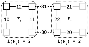
(a) Before merge.

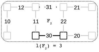
(b) After merge.

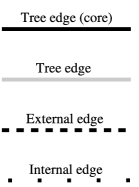
(c)

Figure 1: Example of fragment merge. a) Fragments $F_{0}$ and $F_{1}$ have equal level $l(F_{0})=l(F_{1})=2$. b) A new fragment $F_{2}$ is created and its core is moved towards the joint edge.

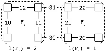
(a) Before absorption.

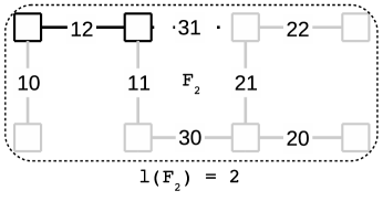
(b) After absorption.

(c)

Figure 2: Example of fragment absorption. a) Fragment $F_{1}$ has lower level than $F_{0}$. b) $F_{1}$ is absorbed by $F_{0}$ creating a new fragment $F_{2}$ which inherits $F_{0}$ core and also its level.

An interesting property of the algorithm is that MST construction is driven by the edge’s weights distribution. Therefore, different weights distributions may achieve different MST configurations.

II-B Ancestor Identification Labeling Scheme

Given the previously computed MST ($T$), we traverse it in a pre-order fashion assigning an integer $a_{i}$ to each traversed vertex $v_{i}$ in a strictly-increasing monotonic order. Additionally, each $v_{i}$ is assigned an integer $b_{i}$ as the maximum $a_{j}$ among all $v_{i}$ successors. Notice that $a_{i}=b_{i}$ if vertex $v_{i}$ is leaf in $T$.

Definition 8.

For each vertex $v_{i}$ of T, there exists a different label $t(v_{i})=[a,b]$ which is a closed integer interval with lower and upper bounds $a$ and $b$ respectively.

By construction, for any given pair of distinct vertices $v_{i}$ and $v_{j}$, this labeling scheme satisfies the following property.

Property 3.

$t(v_{j})\subset t(v_{i})$ iif $v_{i}$ is an ancestor of $v_{j}$. In other words $t(v_{j})$ is a subinterval of $t(v_{i})$.

Using Property 3, the Common Ancestor (CA) definition can be expressed as:

Definition 9.

Given $v_{i},v_{j},v_{k}$ of T, $v_{i}$ is a Common Ancestor (CA) of vertices $v_{j}$ and $v_{k}$ iif $t(v_{j})\subset t(v_{i})$ and $t(v_{k})\subset t(v_{i})$.

Fig. 3 shows an example of label computation in a rooted tree. Intervals lower bound are computed in a pre-order fashion from the tree’s root. Then, upper bounds are computed from leaf vertices towards the root. A similar approach is followed by Santoro et al.[23] to provide an implicit routing for graphs representing arbitrary topologies.

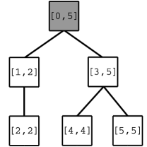
Figure 3: Label computation example.

II-C Segment-based Routing

Segment-based Routing (SR) [14] is a topology-agnostic routing algorithm aimed to provide a reasonable path quality and fault-tolerance while keeping complexity low. SR is considered a rule-driven routing algorithm [24] whose main features and required resources can be summarized as follows:

1. It does not guarantee shortest path computation by design.

2. Virtual channels are not required.

3. Deadlock freedom enforcement and path selection stages do not rely on spanning tree computation.

SR working principle is the partitioning of a topology into subnets. Subnets in turn are made of disjoint segments where routing restrictions are placed locally within each segment to break cycles, thus guaranteeing deadlock freedom and connectivity within each subnet. During the partitioning process, network links are visited at most once to avoid the procedure to reach a deadlocked state.

A segment is defined as a list of interconnected switches and links. Three different segment types can arise from partitioning:

• Starting segment: It starts and ends at the same switch (i.e. it makes a cycle). SR begins the partitioning process by building this segment. Thus, we have to choose a switch (i.e. starting switch) and find a cycle that includes it. The cycle itself is considered the starting segment. There is one starting segment per subnet, which may connect to a different subnet through a bridge link.

• Regular segment: These segments start on a link followed by one or more switches and links, and they end on a link.

• Unitary segment: They are made by a single link.

Guaranteeing deadlock-freedom and connectivity while preserving segments independent from each other, requires the fulfillment of the following construction rules[14]:

Rule 1.

Nodes and links can be included in no more than one segment.

Rule 2.

New regular or unitary segments must be connected to previous constructed segments. Starting segments do not follow this rule.

Fig. 4 shows an example of computed subnets and segments in a 4x3 Mesh with some links missing. In this case, we have four subnets (dashed areas) and three regular segments $S0.0=(\{8,4,5,9\},\{i,f,j,m\})$ , $S3.0=(\{6,7,11,10\},\{h,l,n,k\})$ and $S3.1=(\{2,3\},\{d,b,e\})$. Grayed links joining two subnetworks are not included in any segment, they are considered bridge links.

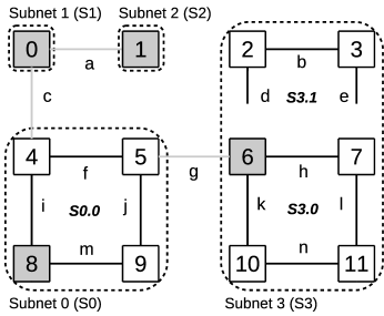
Figure 4: SR partitioning example with four subnets (dashed areas) and three segments S0.0, S3.0 and S3.1. Starting switches within each subnet are filled in gray. Bridge links, namely $a$, $c$ and $g$ are also showed.

In Fig. 4 example, switch 8 was chosen as the starting switch. Then, construction of subnet 0 (S0) begins by building the starting segment within the subnet, that is, finding a cycle from switch 8, yielding segment $S0.0$.

Once the starting segment is found, the algorithm selects among the available outgoing links sourcing previously constructed segments. In this case, only $c$ and $g$ links meet this condition, we choose $c$.

From link $c$, we look for paths ending at any switch within a previous constructed segment. With lack of success, $c$ link is considered a bridge and a new subnet S1 is started, becoming switch 0 the starting switch for the newly created subnet S1.

As each link can be visited only once, to find a cycle from switch 0, we are forced to choose link $a$, where no cycle is found, letting $a$ being a bridge link and a new subnet S2 is started, making switch 1 its starting switch.

In a similar fashion, link $g$ is marked as bridge, triggering the construction of a new subnet S3 with switch 6 as the starting switch. This time, a cycle is found through link $h$ and the starting segment for S3 is built ($S3.0$). Then, we look for available outgoing links sourcing previously constructed segments within the subnet, i.e. $\{d,e\}$ links. By choosing $d$, a path is found to end at a switch already within a previously built segment (switch 7 through $e$), this path becomes the last segment $S3.1$. We provide a detailed SR specification in Appendix A.

III Related Work

Topology-agnostic routing algorithms can be classified in two major categories regarding the computation of the final set of paths between end-points[24]. Path-driven routings achieve this task by selecting among the initial set of paths meeting certain criteria (path length, traffic balance, etc.). The second step focuses on guaranteeing deadlock-freedom, often through the use of virtual-channels to break cyclic path dependencies. TOR[25], LASH[26] and LASH-TOR[27] are some of the routing algorithms falling into the path-driven category.

On the other hand, in rule-driven routings the first step is to achieve deadlock-free routes by the use of rules to break cyclic dependencies, once deadlock freedom is ensured, they must select paths between each source-destination pair to obtain a deterministic routing based upon some criteria (random, round-robin, minimal path, etc.). UD[28], FX[29], LTURN[30], SR[14], Tree-turn Routing[31] and DiSR[32] fall into the rule-driven routing algorithms category.

Due to the nature of the functional steps performed by rule-driven algorithms, they are likely to be implemented in a distributed fashion using only local information at each communication node, i.e. some aspects such as the complete topology and status of the network are not available. Path-driven algorithms, however, require the complete set of paths between each source-destination pair to be able to select among them so as to break cyclic dependencies.

Distributed computation of topology-agnostic routing algorithms enables a more scalable, resilient and flexible routing algorithm. DiSR for instance, is an attempt to achieve the same goals as the SR algorithm but it does not rely on a topology graph nor a centralized computation. Nevertheless, DiSR focuses on fast computation of routing restriction rules rather than guaranteeing connectivity among switches. Thus, leaving unconfigured switches even when computation is performed on a regular topology due to its non-deterministic nature. Traffic routed through unconfigured switches may result in deadlock situations due to the lack of routing restrictions. As a consequence, the system is forced to avoid routing traffic through unconfigured switches.

So far we have discussed deadlock avoidance routing algorithms. Nevertheless, deadlock recovery topology-agnostic mechanisms have also been proposed[33, 34, 35]. These algorithms aim to detect deadlock situations at runtime and recover from it. The reason behind these proposals is that deadlocks are not likely to occur very often. However, tracking network cyclic dependencies require complex logic as well as the mechanism to recover from it. Besides, deadlock detection often relies on counter thresholds which must be properly configured in order to reduce the amount of false positives.

The TDSR approach inherits most of the features of the SR algorithm as well as deadlock avoidance rule-driven algorithms. In addition, TDSR deterministic computation is performed in a completely distributed fashion guaranteeing optimal coverage of switches into segments also in presence of connected components in the topology.

IV Transparent Distributed Segment-Based Routing

In this section we present our proposal, namely Transparent Distributed Segment-Based Routing (TDSR). We give a brief overview of the main goal and features of the proposed distributed algorithm. Then, we provide a detailed explanation of the functional stages performed by TDSR: MST construction, labeling and segment construction.

The main goal of TDSR is devised from the SR[14] original proposal i.e., partitioning of a topology into subnets which, in turn, are further divided in segments.

As we explained in Section II, SR requires the full set of switches and links aimed to be partitioned, then, it starts searching for segments using these two sets. This general approach is not suitable to be carried out in a distributed environment where only local information is available at each communication node (a.k.a. switch). TDSR proposal is a distributed approach to achieve the same objective.

Some SR features are also provided by TDSR:

• It does not guarantee minimal routing by design.

• Virtual channels are not required.

We can split TDSR in three functional stages:

1. MST construction in order to enforce deadlock freedom.

2. Switch labeling to enable Lowest Common Ancestor computation (LCA).

3. Segment construction using the information provided by previous stages.

IV-A Minimum Spanning Tree Construction Stage

TDSR takes advantage of the structure provided by MSTs to identify network links introducing cycles in the network graph (i.e. links not included in the MST). Thus TDSR considers two different types of links, those included in the computed MST (a.k.a. tree links), and those links not included in the MST (a.k.a. internal links). There is also a third link type which arises during the MST construction, called external link. This third type of link connects switches within different fragments of the MST which have yet to be joined (see Section II-A).

We assume that each network link has a different unique weight. Nevertheless, if the previous assumption is not fulfilled, unique link weights can be computed using the identifiers of both switches connected through each link. Then, TDSR uses the GHS distributed algorithm explained in Section II-A to construct the MST.

Fig. 6 shows the Finite-State Machine (FSM) diagram for the MST construction stage. This automata is run by every switch and it consists of three states, namely SLEEPING (SL), FOUND (FO) and FIND (FI). Stage transitions are triggered upon arrival of messages, actions performed within state transitions may involve sending new messages to adjacent switches.

There are eight types of messages involved in the MST construction. Each message type is used at different steps of the procedure. In order to understand each step and the involved messages, we show a small example comprising four switches in a mesh arrangement (see Fig. 5).

Initially all switches are in the SL state and they form a different fragment by themselves of level $0$. All network links are considered External. At any given switch, upon arrival of either a WAKEUP, TEST or CONNECT message, it starts searching for its minimum weight adjacent link. For simplicity we assume that all switches in SL state receive a WAKEUP message to trigger the search for their minimum weight adjacent link.

If no link is found at this point means that the switch is isolated from the network. On the other hand, if a Minimum Weight Link (MWL) is found, the switch sends a CONNECT message containing its level ($0$) through the selected link to join the remote fragment (Fig. 5a). A WAKEUP message is sent through the remaining links (if any) and the switch moves to state FO. Hence, the transition from FSM state SL to FO in Fig. 6 has been accomplished because the MWL has been found within each level 0 fragment.

Each switch eventually receives its corresponding CONNECT message. Then, they answer with an INIT message to merge with the remote fragment as Fig. 5b shows. At this point, two fragments with switches $\{0,2\}$ and $\{1,3\}$ are derived from the merge operation. The INIT message received at each switch causes the transition from state FO to FI. It also changes the link type from external to tree (solid links in the figure) considering it part of the MST.

When transitioning to state FI, switches must find their lower weight adjacent link locally. This is accomplished by sending TEST messages through the lowest weight adjacent link as Fig. 5c shows. TEST messages contain the sender fragment identifier and level. The fragment identifier is the link weight of the fragment core. Hence, fragments $\{0,2\}$ and $\{1,3\}$ identifiers are $10$ and $11$ respectively. For level 0 fragments, no identifiers are considered.

Upon the arrival of a TEST message through an external link, receiving switches may reply either an ACCEPT or REJECT message if the following conditions are met:

1. If fragment identifiers of sender and receiver are equal, a REJECT message is sent back.

2. If fragment identifiers of sender and receiver are different, and sender fragment level is lower or equal than receiver fragment level, an ACCEPT message is sent back.

3. If conditions 1 and 2 are not met, fragment identifiers of sender and receiver must be different and sender fragment has greater level than receiver fragment. In this case, the receiver delays the reply until either condition 1 or 2 is met. Hence, the sender will stall at state FI preventing the greater level fragment to proceed.

Our example has both fragments $\{0,2\}$ and $\{1,3\}$ at the same level ($1$) with different identifiers. Therefore, upon arrival of TEST messages, switches send back an ACCEPT message as Fig. 5d shows. These ACCEPT messages trigger the transition from state FI to state FO which result in REPORT messages being sent towards core switches. REPORT messages contain the MWL found within a branch (see Fig. 5e). Notice that core switches are not considered successors between themselves. Thus, condition All successors (if any) reported? within the transition from state FI to state FO is met (see Fig. 6).

MWL must be located at only one side of the fragment core, in this case, the MWL selected by both fragments is link weighted $12$. Downwards search through neither fragment is needed to locate the MWL because it is located at one of the core switches within each fragment. Otherwise, a CHCORE message would be needed to locate the MWL adjacent switch. Upon reception of a CHCORE message at the MWL adjacent switch (not needed if MWL adjacent switch is within the fragment core), it sends a CONNECT message to merge with the remote fragment (see Fig. 5f).

Upon arrival of CONNECT messages, Fig. 5g shows INIT messages exchanged between remote fragments to create the new fragment resulting from the merge of fragments $\{0,2\}$ and $\{1,3\}$. The new fragment $\{0,1,2,3\}$ has level 2 with edge $12$ as its core. Upon reception of the INIT message, switch move to the FI state to begin searching for a new MWL sending the corresponding TEST messages (see Fig. 5h).

Tested link $13$ has both adjacent switches at the same fragment. Therefore, it is considered an internal link by means of REJECT messages (see Fig. 5i).

Finally, REPORT messages are sent back to the core notifying that no MWL has been found (see Fig. 5j). The MST construction stage finishes upon arrival of REPORT messages with no MWL found at switches through all its downward adjacent edges in the tree as in Fig. 5j. Once core switches receive these REPORT messages through all its adjacent edges (including its sibling core switch), we can safely assume that the final MST has been constructed[15] (i.e. a single fragment remains).

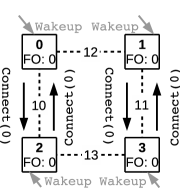
(a)

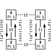
(b)

(c)

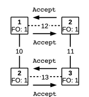
(d)

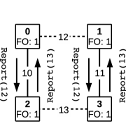
(e)

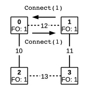
(f)

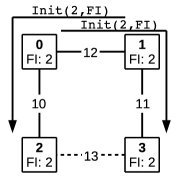
(g)

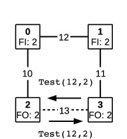
(h)

(i)

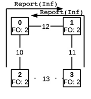
(j)

Figure 5: MST Construction example. a), b) Initial level 0 fragments merge. c), d), e) Level 1 fragments search for outgoing edges. f, g) Level 1 fragments merge. h), i), j) Level 2 fragment tags edge 13 as Internal and finishes.

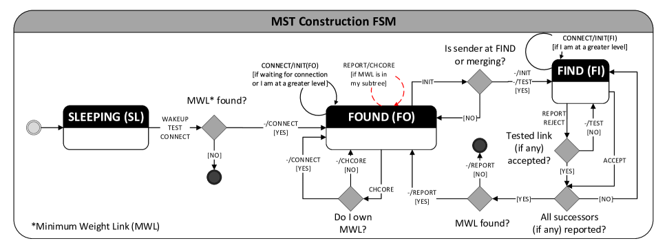
Figure 6: MST Construction FSM diagram.

The MST construction example shown in Fig. 5 puts on display one of the properties mentioned in Section II-A. Edge weights drive the construction of the MST by definition. As a consequence, different MST can be constructed upon different edge weight configurations.

For instance, Fig. 7 shows different MST derived from three different link weight configurations in a $4\times 4$ mesh (grayed switches are one of the core switches chosen as tree root located at the MST core). In Fig. 7a, horizontal edges have lower weight than vertical edges. Also, leftmost edges have a lower weight associated.

On the other hand, Fig. 7b shows an edge weight distribution from the mesh center towards the boundary. Finally, Fig. 7c shows the MST constructed from an edge weight configuration in a zigzag fashion.

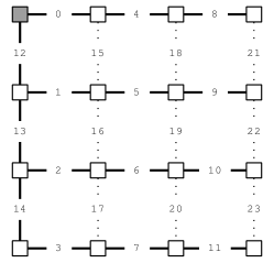
(a) Horizontal distribution

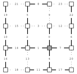
(b) Center distribution

(c) Zigzag distribution

Figure 7: Tree configurations derived from different edge’s weight distributions.

IV-B Labeling Stage

As soon as switches finish the MST Construction Stage (see IV-A), they proceed with the labeling stage. The labeling stage objective is to provide each switch with the necessary information to know whether it is ancestor of any given switch or not. To achieve this, a closed integer interval is associated to each switch, regarded as the switch’s label. A more elaborate explanation of the labeling scheme used is provided in Section II-B.

The finite state machine diagram of this stage’s implementation is provided in Fig. 8. It consists of four states: INIT (IN), COUNT (CO), LABEL (LA) and ACK, each with its corresponding message type named after it.

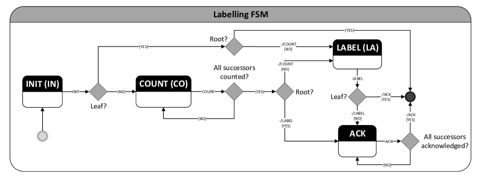
Figure 8: Labeling FSM diagram.

To compute interval lower bounds, each switch must account for the successors in the MST (i.e. using tree links) by means of COUNT messages starting at the leafs, towards the root. Then, an integer value representing the next hop lower bound is sent per downward link starting at the root switch (LABEL messages). For the first downward link considered, the next hop lower bound transmitted must be equal to the switch’s lower bound increased by one.

Lower bounds transmitted through the following downward links are increased by the amount of successors reachable through previously transmitted downward links. This is similar to depth-first search (DFS) traversal algorithm.

Finally, upper bounds are computed at each switch by selecting the maximum lower bound among its successors upon reception of ACK messages from all its successors. Fig. 3 shows an example with switch labels already computed.

Nodes are visited three times: upwards to propagate the amount of successors towards the tree’s root, then, downwards to compute each switch’s label. Finally, ACK messages are transmitted upwards to compute intervals upper bound. Therefore, time complexity upper bound for this stage is $O(3n)$.

IV-C Segment Construction Stage

The segment construction stage objective is to build segments using the internal links (i.e. links not belonging to the MST) arisen from the MST construction stage. The segment build process follows SR construction Rules 1 and 2 discussed in Section II-C to guarantee deadlock-freedom while preserving connectivity. Segments are identified by the weight of the internal link that triggered the segment construction.

Internal links are considered suitable to build a new segment if both endpoints’ Lowest Common Ancestor (LCA) lies within existing segments. Link suitability can be checked by ensuring that switches connected to the constructed segments area (a.k.a. constructed area) but not yet included are not Common Ancestors (CAs) of both link endpoints according to Definition 9. This ensures that the link endpoints LCA lies within the constructed area. Therefore, the new segment will be connected to previous constructed segments and Rule 2 is satisfied.

Fig. 9 shows an example of suitable (left) and unsuitable (right) links. Nodes $A$ and $B$ are connected but not included within the constructed area, because they are not the left link endpoints CAs, left link is considered suitable. $C$, for instance, is not within the constructed area. Nevertheless, $C$ is CA of right link endpoints. In consequence, right link is not suitable to build a segment which connects to already constructed segments.

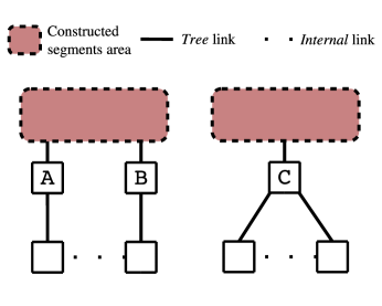
Figure 9: Suitable internal link (left) and an unsuitable internal link (right) to build new segment.

Initially, only the starting switch of the subnet (usually the MST root switch) is considered to be within the constructed area, this allows to build the starting segment.

Switches adjacent to the starting switch (i.e. switches connected to the constructed area, but not included) are used to evaluate internal links suitability in the MST. Internal links endpoints not having any of these adjacent switches as CA are considered suitable to build the starting segment. In other words, suitable internal links endpoints LCA must be the starting switch.

Fig. 10 shows the finite state machine modeling the implemented behavior. This stage takes place after both the MST construction and labeling stages have finished locally at each switch.

The process of checking link suitability and segment building is performed by BUILD and ACK messages, respectively. Nodes in the constructed area (i.e. switches belonging to a constructed segment) send empty BUILD messages through tree links towards switches not included in any segment ($A$ and $B$ in Fig. 9). Directly connected switches to the constructed area found downwards store their label in the BUILD message and keep forwarding it.

Downward internal links check their suitability using the switch’s label provided by the BUILD message (if any), ensuring that this switch is not CA of the internal link endpoints. The BUILD message is forwarded unchanged by intermediate switches towards leaf switches.

Upon arrival of BUILD messages, internal links found (if any) would be considered suitable either if:

1. It has at least one of its endpoints connected directly to the constructed area (BUILD message would be empty at this point).

2. Otherwise, both endpoints must check that the stored switch within the BUILD message is not a CA.

For example, internal link having endpoint switches $A$ and $B$ in Fig. 9 would be suitable because the first condition would be met (i.e. there is at least one endpoint connected directly to the constructed area).

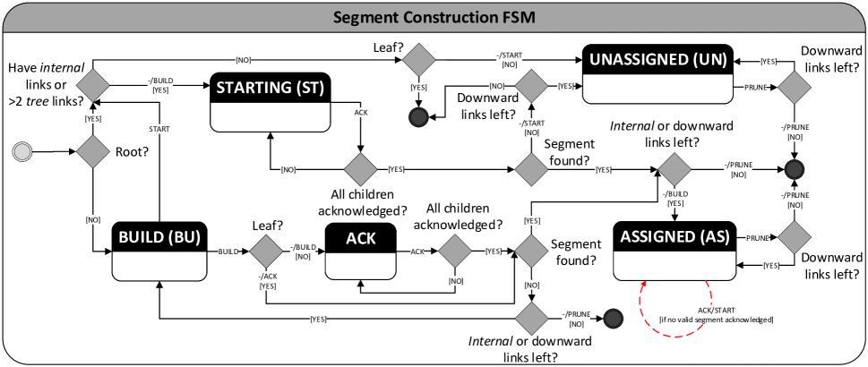
Figure 10: Segment construction FSM diagram.

Leaf switches consume the BUILD message, and they send an ACK message upwards. ACK messages carry the weight of the suitable internal link found (if any).

Along the path traveled by the ACK message, switches and links are assigned to the segment indicated by the ACK message. Paths leading to suitable internal links may overlap. Nevertheless, segment overlapping is not allowed by Rule 1. To avoid segment overlapping, switches wait for arrival of ACK messages from all their successors to be able to select the best link weight stored within all the ACK messages. Finally, upon reception of successors’ ACK messages, an ACK message is sent upwards taking into account the weight of the suitable internal links found at this switch and the best weight selected among its successors.

Fig. 11 shows segments constructed for the tree shown in Fig. 7a. Initial constructed area ($0$) started at root switch. Then, to build segments covering the entire network, the constructed area required three expansions ($1$, $2$ and $3$), each expansion adding new constructed segments. Internal links adding segments in a given area expansion have their LCA endpoints within segments added by the previous expansion. Note that segments do not overlap as lower weight internal links take precedence. The example consists of a single subnet as no bridge links exists.

Upon each segment construction, two routing restrictions (one at each direction) must be placed within the segment to guarantee deadlock-freedom upon routing packets through the network. Although the routing restrictions could be placed anywhere within each segment, for simplicity, we place a bidirectional routing restriction within the switch with lower identifier connected through the internal link upon which the segment was built. However, a different criteria may be used for routing restriction placement within segments.

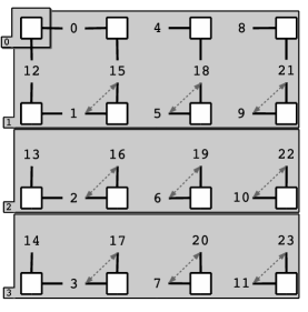
Figure 11: Segment construction example from an horizontal weight distribution MST (see Fig. 7a). Grayed regions show the three area expansions required to build nine segments covering all internal links. Routing restrictions within segments are also shown using dashed arrows.

During segment construction stage, some situations may arise which require a more elaborated explanation. These cases are related to the inability to build new segments:

What if the starting segment cannot be built from the starting switch? Assuming there exists at least one internal link downwards (otherwise, no segments would be built at all), the starting switch withdraws from building the starting segment and sends a START message downwards to its adjacent switches. Then it moves to the UNASSIGNED (UN) state. Downward switches receiving a START message will be considered starting switches to build its starting segment (i.e. they move to state STARTING (ST)). For example, switch $C$ at Fig. 9 shows an example where root switch (assuming the root switch is located within the constructed area) would not be able to build the starting segment. Also, starting switch outgoing links would be considered as bridge links joining different subnets.

What if no segment can be built from the constructed segments area? This situation is observed in Fig. 9 for the unsuitable internal link at the right half of the figure. Similar to the previous situation, we assume that at least one internal link downwards exists. Hence, a START message is sent downwards from the closest switch within the constructed area. This message triggers the construction of a new subnet while searching for the subnet’s starting segment. In Fig. 9, switch $C$ would receive the START message from the constructed area. We can see that the internal link downwards would become a suitable candidate for building the starting segment from $C$. Therefore, a new subnet would be successfully built.

What if no internal links are found? No segments would be built. This case may arise for networks (or network regions) where all available links are tree links. Therefore, by the MST definition, no cycles would exist. Thus, there is no need to build any segment nor place routing restrictions between different links guaranteeing deadlock-freedom and preserving connectivity (provided by tree links within the MST).

Time complexity upper bound for the segment construction stage depends on the number of area expansions required to include existing internal links into segments by having its LCA within the constructed area. Also, for each area expansion, the longest path explored downwards the tree looking for suitable internal links, will have a significant impact on the exploration time required. The worst case scenario would be similar to the tree shown in Fig. 7c, with the root located at one of the two outermost switches. This gives as a result a MST with depth equal to the amount of switches in the network. Then, time complexity upper bound can be safely set as $O(N^{2})$.

V Performance Evaluation

In this section we evaluate TDSR performance in terms of the execution time required for the mechanism to converge to a valid solution in a distributed fashion within different scenarios. Because of the different aspects interacting with TDSR we present the simulation environment and experiment setup details in the following sections.

V-A Simulation Environment

We tested the TDSR mechanism on a cycle-accurate mesh network simulator with the following characteristics:

• Links connecting adjacent switches can transmit at most one packet per cycle.

• Single cycle latency of packet transmission between adjacent switches.

• TDSR control packets cannot be buffered, they must be processed upon arrival.

• TDSR control packet transmission takes precedence over any other packets waiting to be transmitted through the same link.

This environment characterization aims to represent accurately the systems targeted by TDSR such as many-core architectures featuring networks-on-chip[36].

V-B Experiment Setup

The experiment parameters are the network size, defective links percentage over the total amount of links present in the network, and link weight distribution.

Choosing different network sizes for the experiment allows us to test TDSR scalability regarding the amount of switches present in the network. This aspect also depends on the topology properties. Although TDSR is a topology agnostic routing algorithm, for the sake of brevity, only mesh topology is considered as it is a commonly used topology for many-core architectures such as the U.T. Austin Trips[5], Intel Teraflops[6] and Tilera TILE64[7].

The fault model used in the experiment follows a uniform distribution over links between adjacent switches. Due to transistor failures in NoCs, switch’s datapath components are likely to be affected by these faults. Hence, driving individual links unusable[37, 38, 13].

Finally, the link weight distribution dictates the MST structure, which greatly determines the area expansions required to assess link suitability. Refer to Section IV-A for a detailed explanation.

Following, we present the different parameter configurations used in this evaluation.

• Network size: $8\times 8$, $16\times 16$, $32\times 32$ and $64\times 64$.

• Defective link rate: $0\%$ up to $45\%$.

• Link weight distribution: center, horizontal and random. Horizontal and center distributions are shown in Fig. 7a and Fig. 7b respectively. On the other hand, the random link weight distribution has been generated by using a random sample from the available link weights without replacement, ensuring each link gets a different unique weight. The random sample follows a uniform distribution.

V-C Results

The obtained results are shown according to the evaluation metric defined previously, i.e. total execution time (in cycles) of the algorithm.

For the sake of brevity, in this section we only show the results for network size configuration $16\times 16$ (Fig. 12). Besides, we also provide network size configurations $8\times 8$, $32\times 32$ and $64\times 64$ results in Appendix B (Figs. 16, 18 and 19 respectively).

For each network size, we have tested different link weight distributions: center, horizontal and random. Finally, for each link weight distribution, total execution time (vertical axes) is plotted by increasing the defective link rate (horizontal axes).

Given a particular link weight distribution, TDSR operates in a deterministic way. Hence, when no defective links are present in the network, TDSR always converges to the same solution. This is represented by an horizontal line in the results, showing the execution time of TDSR with $0\%$ defective link rate. For defective link rates greater than $0\%$, we run several executions of TDSR by randomly selecting which links will be affected according to the defective rate such as to get a representative sample. This data is plotted using boxplots (a.k.a. Tukey boxplots[39]) in the figures.

(a) Horizontal link weight distribution

(b) Center link weight distribution

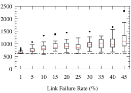
(c) Random link weight distribution

Figure 12: Execution time for 16x16 mesh configuration.

Overall, results show that TDSR needs more cycles to converge if an horizontal link weight distribution is chosen. This happens specially at low defective link rates (see Fig. 12a) within each network size configuration. This is due to the depth of the tree constructed at the MST construction stage, which in most cases is greater than the tree obtained using center and random link weight distributions.

Regarding center and random link weight distributions, TDSR is able to converge to the solution keeping low the execution time compared with the horizontal distribution, specially at low defective link rates. Using the aforementioned distributions, TDSR is less sensitive to an increase in defective link rates up to $20\%$ approximately. Defective link rates above $20\%$ can result in a deeper MST, which in turn raises the convergence time of the mechanism.

Random link weight distribution usually needs more time to finish than center distribution. However, it is less sensitive to faults distributed in a random uniform fashion. This means that the MST depth in presence of defective links does not increase dramatically.

MST and segment construction stages described in sections IV-A and IV-C are the most time consuming stages of TDSR. In the experiment performed, we have found that the segment construction stage usually makes a larger impact on the overall execution time of the mechanism. This stage is also more sensitive than the MST construction stage to the link weight distribution used.

V-D Analysis

A brief discussion about the different aspects driving TDSR performance under certain conditions is necessary.

MST and segment construction stages described in sections IV-A and IV-C are the most time consuming stages of TDSR. In the experiment performed, we have found that the segment construction stage usually makes a larger impact on the overall execution time of the mechanism. This stage is also more sensitive than the MST construction stage to the link weight distribution used. Link weight distribution plays a critical role regarding this aspect, as it determines the MST structure, root location and in consequence, the MST depth. Fig. 13 shows the time each stage needed for the $16\times 16$ mesh configuration.

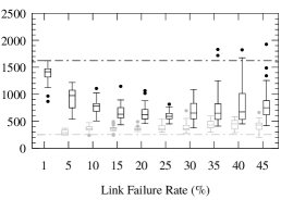
(a) Horizontal link weight distribution

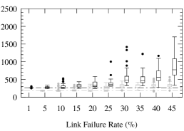
(b) Center link weight distribution

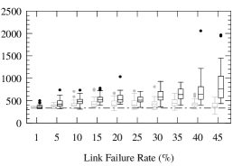
(c) Random link weight distribution

Figure 13: MST and Segment construction stages execution time for 16x16 mesh configuration.

Fig. 14a shows the area expansions required (grayed regions) to build all the segments using a horizontal link weight distribution. Notice the large amount of switch traversals made by TDSR in order to evaluate suitability of the distant internal link (located at the bottom right corner) per area expansion (dashed arrows). Root location within the tree structure generated by the horizontal link weight distribution has a significant impact on the tree depth.

As a consequence, the execution time of TDSR decreases in presence of defective links if using an horizontal link weight distribution (see Fig 12a). This is due to the root location, which in presence of defective links, it may be moved towards the MST center.

On the other hand, if a center link weight distribution is configured, a lower amount of area expansions are required to build the segments. Also, the maximum distance traveled per area expansion is lowered as Fig. 14b shows. In this case, due to the initial centered location of the root with no defective links, the presence of defective links may move the root away from its initial location, thus, increasing the tree depth.

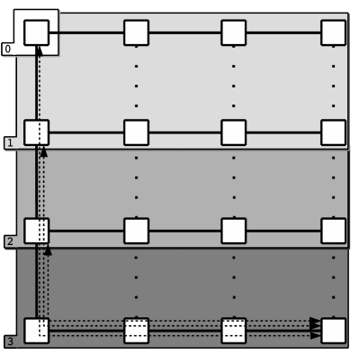
(a)

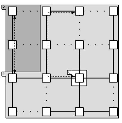
(b)

Figure 14: Area expansions using horizontal (a) and center (b) link weight distribution. Dashed arrows show longest paths explored at each area expansion to construct segments.

Finally, Fig. 15 shows the distance traveled per area expansion in a $16\times 16$ mesh for each link weight distribution with no defective links. The horizontal distribution needs up to 15 area expansions to build the segments with greater distances traveled per area expansion. Meanwhile, center and random distributions keep both factors low, although random distribution may travel slightly greater distances at some area expansions.

Notice that the amount of area expansions required by the horizontal distribution matches the amount of network rows minus one (starting switch area expansion is omitted). This is showed also in Fig. 14a.

Figure 15: Distance traveled per area expansion in a 16x16 mesh using different link weight distribution with no defective links.

VI Conclusion

In this paper we have proposed a new SR-based[14] topology-agnostic deadlock-free distributed algorithm known as Transparent Distributed Segment-based Routing (TDSR).

TDSR algorithm’s main objective is to split the topology in subnets which are further divided in segments in a distributed fashion. Thus, allowing to devise a deadlock-free routing configuration by placing routing restrictions within segments. Moreover, this objective must be achieved guaranteeing connectivity among all switches within the same network component.

Among TDSR key features is the flexibility of segment construction by link weight distribution configuration. Also, depending on the link weight distribution chosen, TDSR outperforms existing proposals such as DiSR[32] in multiple scenarios.

We have analyzed different aspects driving TDSR performance in terms of execution time required to compute all segments. We conclude that choosing an appropriate link weight distribution has a significant impact on the time required by TDSR. Link weight distributions reducing the MST depth provide lower execution time due to its influence on the exploration paths’ length followed per area expansion, and the amount of area expansions required. For instance, defective mesh networks may benefit from a centered link weight distribution.

Future works will focus on setting routing restrictions within segments according to some criteria such as network congestion, flow balancing, etc. This will allow us to study the impact on network performance that the different selection criteria of TDSR may produce.

Strategies to improve TDSR execution time should be further devised, improving those aspects which have a significant impact on performance.

Appendix A Segment-based Routing Pseudocode

Segment-based Routing (SR) [14] is a topology-agnostic routing algorithm aimed to provide a reasonable path quality and fault-tolerance while keeping complexity low. SR is considered a rule-driven routing algorithm [24] whose main features and required resources can be summarized as follows:

1. It does not guarantee shortest path computation by design.

2. Virtual channels are not required.

3. Deadlock freedom enforcement and path selection stages do not rely on spanning tree computation.

SR working principle is the partitioning of a topology into subnets. Subnets in turn are made of disjoint segments where routing restrictions are placed locally within each segment to break cycles, thus guaranteeing deadlock freedom and connectivity within each subnet. During the partitioning process, network links are visited at most once to avoid the procedure to reach a deadlocked state.

A segment is defined as a list of interconnected switches and links. SR pseudocode specification is shown in Algorithm 1. For simplicity, we use helper procedures as described below:

• non_visited_switch: It retreives a non visited switch from either a set of Switches or a particular link.

• outgoing_links: Given a set of switches within a subnet, it retrieves the outgoing links from that subnet (i.e. links connecting a switch within the subnet, with a foreign switch which is not contained in that subnet).

• path_to_segment: It returns the set of switches and links traversed starting at a link in a subnet to form a segment (i.e. it must finish in an already computed segment within the same subnet).

$S$ the set of Switches, $L$ the set of Links

procedure SR($S$, $L$)

     $B\leftarrow\emptyset$$\triangleright$ The set of bridge links

     $sn\leftarrow 0$$\triangleright$ Subnet counter

     $sg\leftarrow 0$$\triangleright$ Segment counter

     $SG_{s}[sn][sg]\leftarrow\emptyset$ $\triangleright$ Segment switches per subnet

     $SG_{l}[sn][sg]\leftarrow\emptyset$ $\triangleright$ Segment links per subnet

     while $|SG_{l}|\neq|L|\land|SG_{s}|\neq|S|$ do

         if $B=\emptyset$ then

              $s\leftarrow non\_visited\_switch(S)$

         else

              $s\leftarrow non\_visited\_switch(link):link\in B$

         end if

         $SG_{s}[sn][sg]\leftarrow SG_{s}[sn][sg]+s$

         for $link\in outgoing\_links(SG_{s}[sn])$ do

              $S^{\prime},L^{\prime}\leftarrow path\_to\_segment(link,SG_{s}[sn])$

              if $L^{\prime}\neq\emptyset$ then

                  $SG_{l}[sn][sg]\leftarrow SG_{l}[sn][sg]+L^{\prime}$

                  $SG_{s}[sn][sg]\leftarrow SG_{s}[sn][sg]+S^{\prime}$

                  $sg\leftarrow sg+1$

              else

                  $B\leftarrow B+link$

              end if

         end for

         $sn\leftarrow sn+1$

         $sg\leftarrow 0$

     end while

end procedure

Algorithm 1 Segment-based Routing.

Appendix B Additional Results

The obtained results are shown according to the evaluation metric defined previously, i.e. total execution time (in cycles) of the algorithm.

Results are drawn for each network size configuration: $8\times 8$ (Fig. 16), $16\times 16$ (Fig. 17), $32\times 32$ (Fig. 18) and $64\times 64$ (Fig. 19). For each network size, we have tested different link weight distributions: center, horizontal and random. Finally, for each link weight distribution, total execution time (vertical axes) is plotted by increasing the defective link rate (horizontal axes).

Given a particular link weight distribution, TDSR operates in a deterministic way. Hence, when no defective links are present in the network, TDSR always converges to the same solution. This is represented by an horizontal line in the results, showing the execution time of TDSR with $0\%$ defective link rate. For defective link rates greater than $0\%$, we run several executions of TDSR by randomly selecting which links will be affected according to the defective rate such as to get a representative sample.

(a) Horizontal link weight distribution

(b) Center link weight distribution

(c) Random link weight distribution

Figure 16: Execution time for 8x8 mesh configuration.

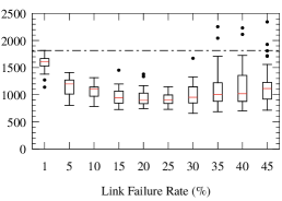
(a) Horizontal link weight distribution

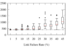
(b) Center link weight distribution

(c) Random link weight distribution

Figure 17: Execution time for 16x16 mesh configuration.

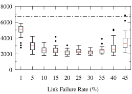
(a) Horizontal link weight distribution

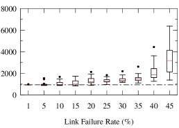
(b) Center link weight distribution

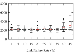
(c) Random link weight distribution

Figure 18: Execution time for 32x32 mesh configuration.

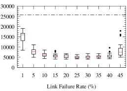
(a) Horizontal link weight distribution

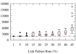
(b) Center link weight distribution

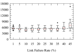
(c) Random link weight distribution

Figure 19: Execution time for 64x64 mesh configuration.

Overall, results show that TDSR needs more cycles to converge if an horizontal link weight distribution is chosen. This happens specially at low defective link rates (see Figs. 16a, 17a and 18a) within each network size configuration. This is due to the depth of the tree constructed at the MST construction stage, which in most cases is greater than the tree obtained using center and random link weight distributions.

Regarding center and random link weight distributions, TDSR is able to converge to the solution keeping low the execution time compared with the horizontal distribution, specially at low defective link rates. Using the aforementioned distributions, TDSR is less sensitive to an increase in defective link rates up to $20\%$ approximately. Defective link rates above $20\%$ can result in a deeper MST, which in turn raises the convergence time of the mechanism. Random link weight distribution usually needs more time to finish than center distribution. However, it is less sensitive to faults distributed in a random uniform fashion (i.e. lower MST depth).

References

- [1] The InfiniBand® Architecture Specification, Volume 1, Release 1.3. The InfiniBand Trade Association, March 2015. [Online]. Available: http://www.infinibandta.org
- [2] “Top500 supercomputer list,” https://www.top500.org/lists/2019/06/, 53rd edition, June 2019.
- [3] T. Nordström and B. Svensson, “Using and designing massively parallel computers for artificial neural networks,” Journal of parallel and distributed computing, vol. 14, no. 3, pp. 260–285, 1992.
- [4] K. De Raedt, K. Michielsen, H. De Raedt, B. Trieu, G. Arnold, M. Richter, T. Lippert, H. Watanabe, and N. Ito, “Massively parallel quantum computer simulator,” Computer Physics Communications, vol. 176, no. 2, pp. 121–136, 2007.
- [5] P. Gratz, C. Kim, K. Sankaralingam, H. Hanson, P. Shivakumar, S. W. Keckler, and D. Burger, “On-chip interconnection networks of the trips chip,” IEEE Micro, vol. 27, no. 5, pp. 41–50, 2007.
- [6] S. Vangal, J. Howard, G. Ruhl, S. Dighe, H. Wilson, J. Tschanz, D. Finan, P. Iyer, A. Singh, T. Jacob et al., “An 80-tile 1.28 tflops network-on-chip in 65nm cmos,” in 2007 IEEE International Solid-State Circuits Conference. Digest of Technical Papers. IEEE, 2007, pp. 98–589.
- [7] D. Wentzlaff, P. Griffin, H. Hoffmann, L. Bao, B. Edwards, C. Ramey, M. Mattina, C.-C. Miao, J. F. Brown III, and A. Agarwal, “On-chip interconnection architecture of the tile processor,” IEEE micro, no. 5, pp. 15–31, 2007.
- [8] A. Sodani, R. Gramunt, J. Corbal, H.-S. Kim, K. Vinod, S. Chinthamani, S. Hutsell, R. Agarwal, and Y.-C. Liu, “Knights landing: Second-generation intel xeon phi product,” Ieee micro, vol. 36, no. 2, pp. 34–46, 2016.
- [9] J.-P. Fricker and P. Ferolito, “Apparatus and method for multi-die interconnection,” Jul. 30 2019, uS Patent App. 10/366,967.
- [10] H. Esmaeilzadeh, E. Blem, R. S. Amant, K. Sankaralingam, and D. Burger, “Dark silicon and the end of multicore scaling,” in 2011 38th Annual international symposium on computer architecture (ISCA). IEEE, 2011, pp. 365–376.
- [11] M. Haselman and S. Hauck, “The future of integrated circuits: A survey of nanoelectronics,” Proceedings of the IEEE, vol. 98, no. 1, pp. 11–38, 2009.
- [12] O. Lysne, J. M. Montanana, J. Flich, J. Duato, T. M. Pinkston, and T. Skeie, “An efficient and deadlock-free network reconfiguration protocol,” IEEE Transactions on Computers, vol. 57, no. 6, pp. 762–779, 2008.
- [13] D. Lee, R. Parikh, and V. Bertacco, “Brisk and limited-impact noc routing reconfiguration,” in 2014 Design, Automation & Test in Europe Conference & Exhibition (DATE). IEEE, 2014, pp. 1–6.
- [14] A. Mejia, J. Flich, J. Duato, S.-A. Reinemo, and T. Skeie, “Segment-based routing: An efficient fault-tolerant routing algorithm for meshes and tori,” in Proceedings 20th IEEE International Parallel & Distributed Processing Symposium. IEEE, 2006, pp. 10–pp.
- [15] R. G. Gallager, P. A. Humblet, and P. M. Spira, “A distributed algorithm for minimum-weight spanning trees,” ACM Transactions on Programming Languages and systems (TOPLAS), vol. 5, no. 1, pp. 66–77, 1983.
- [16] J. Nešetřil, E. Milková, and H. Nešetřilová, “Otakar borůvka on minimum spanning tree problem translation of both the 1926 papers, comments, history,” Discrete mathematics, vol. 233, no. 1-3, pp. 3–36, 2001.
- [17] R. C. Prim, “Shortest connection networks and some generalizations,” The Bell System Technical Journal, vol. 36, no. 6, pp. 1389–1401, 1957.
- [18] J. B. Kruskal, “On the shortest spanning subtree of a graph and the traveling salesman problem,” Proceedings of the American Mathematical society, vol. 7, no. 1, pp. 48–50, 1956.
- [19] S. Chung and A. Condon, “Parallel implementation of bouvka’s minimum spanning tree algorithm,” in Proceedings of International Conference on Parallel Processing. IEEE, 1996, pp. 302–308.
- [20] P. Spira, “Communication complexity of distributed minimum spanning tree algorithms,” in Proceedings of the second Berkeley conference on distributed data management and computer networks, 1977.
- [21] B. Awerbuch, “Optimal distributed algorithms for minimum weight spanning tree, counting, leader election, and related problems,” in Proceedings of the nineteenth annual ACM symposium on Theory of computing. ACM, 1987, pp. 230–240.
- [22] J. A. Garay, S. Kutten, and D. Peleg, “A sublinear time distributed algorithm for minimum-weight spanning trees,” SIAM Journal on Computing, vol. 27, no. 1, pp. 302–316, 1998.
- [23] N. Santoro and R. Khatib, “Labelling and implicit routing in networks,” The computer journal, vol. 28, no. 1, pp. 5–8, 1985.
- [24] J. Flich, T. Skeie, A. Mejia, O. Lysne, P. Lopez, A. Robles, J. Duato, M. Koibuchi, T. Rokicki, and J. C. Sancho, “A survey and evaluation of topology-agnostic deterministic routing algorithms,” IEEE Transactions on Parallel and Distributed Systems, vol. 23, no. 3, pp. 405–425, 2011.
- [25] J. C. Sancho, A. Robles, J. Flich, P. Lopez, and J. Duato, “Effective methodology for deadlock-free minimal routing in infiniband networks,” in Proceedings International Conference on Parallel Processing. IEEE, 2002, pp. 409–418.
- [26] T. Skeie, O. Lysne, and I. Theiss, “Layered shortest path (lash) routing in irregular system area networks,” in ipdps. Citeseer, 2002, p. 0162.
- [27] T. Skeie, O. Lysne, J. Flich, P. Lopez, A. Robles, and J. Duato, “Lash-tor: A generic transition-oriented routing algorithm,” in Proceedings. Tenth International Conference on Parallel and Distributed Systems, 2004. ICPADS 2004. IEEE, 2004, pp. 595–604.
- [28] M. D. Schroeder, A. D. Birrell, M. Burrows, H. Murray, R. M. Needham, T. L. Rodeheffer, E. H. Satterthwaite, and C. P. Thacker, “Autonet: A high-speed, self-configuring local area network using point-to-point links,” IEEE Journal on Selected Areas in Communications, vol. 9, no. 8, pp. 1318–1335, 1991.
- [29] J. C. Sancho, A. Robles, and J. Duato, “A flexible routing scheme for networks of workstations,” in International Symposium on High Performance Computing. Springer, 2000, pp. 260–267.
- [30] M. Koibuchi, A. Funahashi, A. Jouraku, and H. Amano, “L-turn routing: An adaptive routing in irregular networks,” in International Conference on Parallel Processing, 2001. IEEE, 2001, pp. 383–392.
- [31] J. Zhou and Y.-C. Chung, “Tree-turn routing: an efficient deadlock-free routing algorithm for irregular networks,” The Journal of Supercomputing, vol. 59, no. 2, pp. 882–900, 2012.
- [32] V. Catania, A. Mineo, S. Monteleone, and D. Patti, “Distributed topology discovery in self-assembled nano network-on-chip,” Computers & Electrical Engineering, vol. 40, no. 8, pp. 292–306, 2014.
- [33] K. Anjan and T. M. Pinkston, “An efficient, fully adaptive deadlock recovery scheme: Disha,” in ACM SIGARCH Computer Architecture News, vol. 23, no. 2. ACM, 1995, pp. 201–210.
- [34] A. Ramrakhyani and T. Krishna, “Static bubble: A framework for deadlock-free irregular on-chip topologies,” in 2017 IEEE International Symposium on High Performance Computer Architecture (HPCA). IEEE, 2017, pp. 253–264.
- [35] A. Ramrakhyani, P. V. Gratz, and T. Krishna, “Synchronized progress in interconnection networks (spin): A new theory for deadlock freedom,” in 2018 ACM/IEEE 45th Annual International Symposium on Computer Architecture (ISCA). IEEE, 2018, pp. 699–711.
- [36] J. Flich, G. Agosta, P. Ampletzer, D. A. Alonso, C. Brandolese, E. Cappe, A. Cilardo, L. Dragić, A. Dray, A. Duspara et al., “Exploring manycore architectures for next-generation hpc systems through the mango approach,” Microprocessors and Microsystems, vol. 61, pp. 154–170, 2018.
- [37] D. Fick, A. DeOrio, J. Hu, V. Bertacco, D. Blaauw, and D. Sylvester, “Vicis: a reliable network for unreliable silicon,” in Proceedings of the 46th Annual Design Automation Conference. ACM, 2009, pp. 812–817.
- [38] K. Aisopos, A. DeOrio, L.-S. Peh, and V. Bertacco, “Ariadne: Agnostic reconfiguration in a disconnected network environment,” in 2011 International Conference on Parallel Architectures and Compilation Techniques. IEEE, 2011, pp. 298–309.
- [39] M. Frigge, D. C. Hoaglin, and B. Iglewicz, “Some implementations of the boxplot,” The American Statistician, vol. 43, no. 1, pp. 50–54, 1989.