Physically motivated heat conduction treatment in simulations of solar–like stars: effects on dynamo transitions

Abstract

Context. Results from global magnetoconvection simulations of solar-like stars are at odds with observations in many respects: They show a surplus of energy in the kinetic power spectrum at large scales, anti-solar differential rotation profiles, with accelerated poles and a slow equator, for the solar rotation rate, and a transition from axi– to non–axisymmetric dynamos at a much lower rotation rate than what is observed. Even though the simulations reproduce the observed active longitudes in fast rotators, their motion in the rotational frame (the so–called azimuthal dynamo wave, ADW) is retrograde, in contrast to the prevalent prograde motion in observations.

Aims. We study the effect of a more realistic treatment of heat conductivity in alleviating the discrepancies between observations and simulations.

Methods. We use physically–motivated heat conduction, by applying Kramers opacity law, on a semi–global spherical setup describing convective envelopes of solar-like stars, instead of a prescribed heat conduction profile from mixing–length arguments.

Results. We find that some aspects of the results now better correspond to observations: The axi– to non–axisymmetric transition point is shifted towards higher rotation rates. We also find a change in the propagation direction of ADWs so that also prograde waves are now found. The transition from anti–solar to solar–like rotation profile, however, is also shifted towards higher rotation rates, leaving the models into an even more unrealistic regime.

Conclusions. Although a Kramers–based heat conduction does not help in reproducing the solar rotation profile, it does help in the faster rotation regime, where the dynamo solutions now match better with observations.

1 Introduction

The solar surface differential rotation has been known for a long time (Scheiner 1630; Carrington 1863): the equator completes a turn in around 25 days, while the poles take roughly 30 days. Helioseismic inferences have allowed also to uncover the subsurface rotation (Schou et al. 1998), and revealed that the lines of constant angular velocity are radial. This was somewhat unexpected, as in a uniform, incompressible flow, the Taylor–Proudman theorem (Chandrasekhar 1961) states that the horizontal components of the velocity field cannot vary in the direction of the rotation axis, and the flow is forced to move in vertical columns, in which case angular velocity contours constant on cylinders would be observed. Hence, the Sun is able to break the Taylor–Proudman balance with some means. Another surprising observational result came from time-distance helioseismology (Hanasoge et al. 2012), which revealed a lack of power in the kinetic energy spectrum at large scales, where the peak for giant cells should be located. Such a peak would be expected from mixing–length theory (MLT; Vitense 1953; Böhm-Vitense 1958): in its original formulation, MLT predicts convection at all possible scales, which would also correspond to cells of the diameter of the entire convective layer. Also, more recent measurements (e.g., Rincon et al. 2017) suggest that supergranulation may indeed be the largest scale excited in the Sun.

Theoretical explanations as to how the Sun breaks the Taylor–Proudman balance include a ”thermal wind”, generating a clockwise meridional circulation pattern. This circulation results from a latitudinal temperature gradient, which is such that the pole is warmer than the equator by a small amount, of the order of a few Kelvin (Rüdiger 1989). This temperature difference is comparable to the error of current instruments, although Rast et al. (2008) reported on an enhancement of $\sim 2.5\leavevmode\nobreak\ {\rm K}$ at the Sun’s poles. One possibility to explain such a temperature gradient theoretically is to argue for the importance of turbulent effects, such as latitudinally anisotropic heat flux, which has been shown to be able to lead to a temperature difference of $\sim 4\leavevmode\nobreak\ {\rm K}$ (Kitchatinov & Rüdiger 1995). Also, the presence of a weakly subadiabatic layer at the base of the convection zone has been shown to generate a thermal wind and sustain the necessary temperature gradient in a mean–field hydrodynamic model (Rempel 2005).

Modelling efforts of stellar convection in spherical or semi–spherical shells still struggle in producing solutions in which the Taylor-Proudman balance is self–consistently broken, and thus still tend to show cylindrical isocontours for the differential rotation (e.g., Guerrero et al. 2013; Gastine et al. 2014; Käpylä et al. 2014; Augustson et al. 2015). This is commonly interpreted to imply too strong a rotational influence. Moreover, such models are unable to reproduce an accelerated equator when using the solar rotation rate (Gastine et al. 2014; Käpylä et al. 2014; Karak et al. 2015). Most of present–day numerical setups are using fixed heat conduction profiles and depths of convection zones (e.g., Brun et al. 2011; Käpylä et al. 2013), motivated by MLT. Although MLT–designed setups have been successful in reproducing the pattern of granulation and supergranulation in surface convection (e.g., Brandenburg et al. 2005; Nordlund et al. 2009), models simulating deeper parts of the convection zone (CZ) produce far more power in the velocity spectrum at large scale than observations (Gizon & Birch 2012). All the above mentioned discrepancies between observations and numerical models are collectively known as “convective conundrum” (see, e.g., O’Mara et al. 2016) and solving it is one of the major challenges of contemporary solar physics.

One proposed way to crack the convective conundrum is to hypothesize that the actual convectively unstable layer in the Sun, according to the Schwarzschild criterion (Chandrasekhar 1961), is shallower than expected. Spruit (1997) described convection as being driven by cool threads descending from the surface into deeper layers, overwhelming the convection driven by heating from below. Such a phenomenon is now denoted as entropy rain (Brandenburg 2016) and describes surface–driven convection, that would excite only small to medium length scales. By extending MLT to include entropy fluctuations, Brandenburg (2016) identified the presence of a Schwarzschild stable, sub–adiabatic, layer in which the convective flux is still positive. Such a layer was identified first in the Earth’s atmosphere (Deardorff 1961, 1966), and hence was termed as “Deardorff layer”.

The formation of such sub–adiabatic layers has been reported in the hydrodynamic studies of, e.g., Hotta (2017), Korre et al. (2017), and Käpylä et al. (2017). Especially the study by Käpylä et al. (2017) is relevant here, as they demonstrated the emergence of a substantial sub–adiabatic layer, and the existence of non–local surface driving of convection, by using Kramers opacity law in a Cartesian model. Consequently, they redefined the convection zone as the sum of the convection zone in the traditional sense, now called buoyancy zone, plus the sub–adiabatic part, now denoted as Deardorff layer. The depth of the layers was not determined a priori, but rather was an outcome of the simulations.

However, these studies did not investigate large–scale dynamo action. The effect of sub–adiabatic layers in global MHD simulations was investigated by Käpylä et al. (2019). The formation of a stably stratified layer at the bottom of the domain allowed for the storage of magnetic field beneath it, also found in an earlier study by (Browning et al. 2006), but these strong fields were also observed to be capable of suppressing the oscillating magnetic field at the surface. Käpylä et al. (2019) also considered the effect of sub–adiabatic layers on the convective velocity spectra, but found that the decrease in power at large scales was not enough to solve this part of the conundrum.

Another mechanism to reduce the too high rotational influence on convection in simulations, studied first in a Cartesian model by Hotta et al. (2015) and then in fully spherical models by Karak et al. (2018), could be provided by the Lorentz force feedback from the magnetic to the velocity field. Such feedback could result from strong magnetic fluctuations, originating e.g., from the action of a small–scale dynamo instability (see, e.g., Kazantsev 1968) operating the the CZ. Thereby generated magnetic fluctuations could suppress the turbulent velocity field through the Lorentz force, hence acting as an enhanced viscosity, and increasing the magnetic Prandtl number, the ratio of the viscosity and resistivity of the fluid. Karak et al. (2018) investigated such a situation numerically, and their simulations developed an overshoot zone at the base of the domain, and also showed a decrease in the convective power at large scales, due to downward directed plumes. These results, although arising for a different reason, are consistent with the results of Käpylä et al. (2017) and Käpylä et al. (2019). Another finding of Karak et al. (2018) was that the plumes, carrying their angular momentum inward, caused the rotation profile to switch to anti–solar.

Observations of rapidly rotating stars, younger and more active than the Sun, indicate concentrations of magnetic activity at high latitudes persisting for a long time (e.g., Berdyugina & Tuominen 1998). A common configuration is two activity patches on two “active” longitudes, separated roughly by 180 degrees in longitude (e.g., Jetsu 1996). Active longitudes usually migrate in the rotational frame of the star, forming azimuthal dynamo waves (ADW) (e.g., Berdyugina & Tuominen 1998). The direction of migration of these structures can follow the plasma rotation, and in this case we will talk about prograde ADWs; they can also drift in the opposite direction (retrograde ADWs), or they can stand still with respect to the observer’s point of view (standing ADW). These ADWs can persist for time spans extending to ten years (e.g., Lindborg et al. 2011), or their appearance can be more erratic (e.g., Olspert et al. 2015), with a short–lived ADW reappearing after some time. Lehtinen et al. (2016) and See et al. (2016) reported on a threshold in activity, above which stars show active longitudes. In the study of Lehtinen et al. (2016), the active longitudes found were mostly migrating in the prograde direction. The appearance of active longitudes has been attributed to non–axisymmetric dynamo modes operating in these stars (Tuominen et al. 2002), in contrast to the axisymmetric dynamo operating in less active stars. The transition from non–axisymmetric to axisymmetric dynamos has also been studied numerically (Cole et al. 2014; Viviani et al. 2018), but these studies reported a majority of retrograde ADWs, and a transition from axi– to non–axisymmetric solutions at too low rotation rates in comparison to observations. Both studies were using prescribed and MLT-motivated profiles for heat conduction, resulting in a priori fixed depth of the convection zone.

The aim of this paper is to extend the study of Viviani et al. (2018) to include a dynamically adaptable heat conduction. In order to do this, we use a Kramers–like opacity law, as was done in Käpylä et al. (2019) for semi–spherical wedge simulations. We use computational domains extending over the full longitudinal extent to be able to study both axi– and non–axisymmetric dynamo solutions.

2 Setup and Model

We apply a similar setup as in Käpylä et al. (2013) and Käpylä et al. (2019), representing the outer envelope of a solar-like star, $0.7R\leq r\leq R$ (with $R$ the radius of the star), in a semi–spherical domain, $0\leq\phi\leq 2\pi$ and $\theta_{0}\leq\theta\leq\pi-\theta_{0}$ ($\theta_{0}=15^{o}$). We solve numerically the system of MHD equations:

$$\frac{{\rm D}\rm ln\rho}{{\rm D}t} +\nabla\cdot{\bm{U}}=0,$$ (1)

$$\frac{{\rm D}{\bm{U}}}{{\rm D}t} =\mbox{\boldmath$g$}{}-2\bm{\Omega}_{0}\times{\bm{U}}+\frac{1}{\rho}\left({\bm{J}}\times{\bm{B}}-\nabla p+\nabla\cdot 2\nu\rho\bm{\mathsf{S}}\right),$$

$$T\frac{{\rm D}s}{{\rm D}t} =\frac{1}{\rho}\left[-\nabla\cdot\left({\bm{F}}^{\rm rad}+{\bm{F}}^{\rm SGS}\right)+\mu_{0}\eta{\bm{J}}^{2}-\Gamma_{\rm cool}\right]+2\nu\bm{\mathsf{S}}^{2},$$

$$\frac{\partial{\bm{A}}}{\partial t} ={\bm{U}}\times{\bm{B}}-\mu_{0}\eta{\bm{J}},$$

where $\rho$ and ${\bm{U}}$ are the density and the velocity field, $\mbox{\boldmath$g$}{}=-GM/r^{3}$ is the gravitational acceleration, with $G$ being the gravitational constant and $M$ the mass of the star. $\bm{\Omega}_{0}=\Omega_{0}\left(\cos\theta,-\sin\theta,0\right)$ is the bulk rotation. ${\bm{J}}$, ${\bm{B}}$ and ${\bm{A}}$ are the electric current, the magnetic field and the vector potential, respectively, $p$, $\nu$ and $\mu_{0}$ are the pressure, the viscosity, and the magnetic permeability in vacuum, while $\eta$ is the magnetic diffusivity. $\bm{\mathsf{S}}$ is the rate–of–strain tensor. ${\bm{F}}^{\rm rad}$ and ${\bm{F}}^{\rm SGS}$ are the radiative and sub–grid scale (SGS) fluxes, expressed by:

$${\bm{F}}^{\rm rad}=-K\nabla T\quad{\bm{F}}^{\rm SGS}=-\chi_{\rm SGS}\rho T\nabla s^{\prime}\quad.$$ (2)

$K$ is the radiative heat conductivity and $\chi_{\rm SGS}$ is the SGS heat diffusivity, assumed to be constant. $s^{\prime}$ is the fluctuating entropy, $s^{\prime}=s-\left\langle\overline{s}\right\rangle_{\theta}$, where the overbar denotes longitudinal average and the brackets express averaging over the variable in the subscript. Finally, $\Gamma_{\rm cool}$ is a term acting near the surface and cooling towards a reference temperature. Its flux is expressed as:

$$\overline{F}_{\rm cool}=\int_{0.7R}^{R}\Gamma_{\rm cool}dr.$$ (3)

The initial velocity and magnetic fields are gaussian seeds. The initial stratification is isentropic. The radiative heat conductivity, $K$, follows from Kramers opacity law for free–free and bound–free transitions (used also in Barekat & Brandenburg 2014; Käpylä et al. 2017; Käpylä 2019; Käpylä et al. 2019, 2020):

$$K=K_{0}\left(\frac{\rho}{\rho_{0}}\right)^{2}\left(\frac{T}{T_{0}}\right)^{13/2},$$ (4)

where $\rho_{0}$ and $T_{0}$ are reference values for density and temperature. The constant $K_{0}$ is defined via:

$$K_{0} =\frac{\mathcal{L}}{4\pi}c_{v}\left(\gamma-1\right)\left(n_{\rm ad}+1\right)\rho_{0}\sqrt{GMR},$$ (5)

$$\mathcal{L} =\frac{L_{0}}{\rho_{0}\left(GM\right)^{3/2}R^{1/2}}.$$

$\mathcal{L}$ is the normalized luminosity, $c_{\rm V}$ is the specific heat at constant volume, $\gamma=c_{\rm P}/c_{\rm V}$ is the ratio between the specific heat at constant pressure and volume, and $n_{\rm ad}=1.5$ is the adiabatic index.

The velocity field is impenetrable and stress free at all boundaries, while entropy derivatives are set to zero at $\theta=\theta_{0}$ and $\theta=\pi-\theta_{0}$. The magnetic field is radial at $r=R$ and a perfect conductor boundary condition is applied at the bottom boundary. At the latitudinal boundaries, ${\bm{B}}$ is tangential, which means, in terms of the vector potential:

$$A_{r}=A_{\phi}=\frac{\partial A_{\theta}}{\partial\theta}=0\qquad{\rm at}\quad\theta=\theta_{0}\quad{\rm and}\quad\theta=\pi-\theta_{0}$$ (6)

Käpylä et al. (2020) showed that this latitudinal boundary condition does not generate major differences with respect to the perfect conductor boundary condition used in previous works (e.g., in Käpylä et al. 2013; Cole et al. 2014; Warnecke et al. 2014; Viviani et al. 2018).

The simulations are defined by the parameters $\Omega_{0}$, $\nu$, $\eta$, $\chi_{\rm SGS}$, $K_{0}$, $\rho_{0}$, $T_{0}$ and the energy flux at the bottom, $F_{\rm bot}=-K\partial_{r}T|_{r=0.7R}$.

Moreover, important non–dimensional input parameters are the magnetic and SGS Prandtl numbers:

$${\rm Pr}_{\rm M}=\frac{\nu}{\eta},\quad{\rm Pr}_{\rm SGS}=\frac{\nu}{\chi_{\rm SGS}}.$$ (7)

Output parameters of the simulations are the fluid and magnetic Reynolds numbers:

$${\rm Re}=\frac{u_{\rm rms}}{\nu k_{f}},\quad{\rm Rm}=\frac{u_{\rm rms}}{\eta k_{f}}$$ (8)

with $u_{\rm rms}=\sqrt{3/2\left\langle U_{r}^{2}+U_{\theta}^{2}\right\rangle_{r\theta\phi t}}$ rms velocity and $k_{f}=2\pi/0.3R$ the wavenumber of the largest eddy, corresponding to the radial extent, and the Coriolis number:

$${\rm Co}=\frac{2\Omega_{0}}{u_{\rm rms}k_{f}},$$ (9)

quantifying the relative importance of rotation and convection.

Physical units are chosen using the solar radius $R=7\cdot 10^{8}\leavevmode\nobreak\ {\rm m}$, the solar angular velocity $\Omega_{\odot}=2.7\cdot 10^{-6}\leavevmode\nobreak\ {\rm s^{-1}}$, the density at the bottom of the solar convection zone $\rho_{\rm bot}=200\leavevmode\nobreak\ {\rm Kg\leavevmode\nobreak\ m^{-3}}$, and the magnetic permeability in vacuum $\mu_{0}=4\pi\cdot 10^{-7}\leavevmode\nobreak\ {\rm H\leavevmode\nobreak\ m^{-1}}$. We performed our simulations using the Pencil Code, a high–order, finite–difference, open source code for solving the magnetohydrodynamic equations.

3 Results

The simulations and their defining parameters are summarized in Table 1. Run R1 and R2 correspond to Run C3 and D of Viviani et al. (2018), where the radiative heat conductivity K was only a function of depth, as described in Käpylä et al. (2013). Here, our aim is to study the effect of the more physical treatment for heat conduction on the anti–solar to solar–like differential rotation transition and the transition to non–axisymmetric magnetic fields. Run C3 was the simulation with the slowest rotation rate showing both accelerated equator and non-axisymmetric magnetic field, hence it is a good choice for this study. Run D had a rotation rate 2.1 times the solar value, exhibited a non-oscillatory dynamo solution with dominance of the $m=1$ Fourier mode with a retrograde ADW; Run C3 behaved otherwise similarly, but the dynamo solution was oscillatory. This difference in between the runs was most likely connected to the higher amount of differential rotation in C3 than in D, see also Sect.A, where we reproduce the rotation profiles of these runs. Run R3 is the extension of the three times solar rotation rate Run MHD2 of Käpylä et al. (2019) over the full longitudinal extent. Run MHD2 was a wedge simulation covering 1/4 of the full longitude, hence not allowing for non–axisymmetric solutions to develop. We repeat this run in an extended azimuthal domain to study the possible topological changes of the magnetic field. Run R4 has the same setup as Run R3, but twice the rotation rate. Simulations in the same rotation range, but with fixed heat conduction profiles (e.g., Viviani et al. 2018), all showed a clear dominance of the non–axisymmetric mode over the axisymmetric one, and ADWs with retrograde migration.

Run	$\Omega[\Omega_{\odot}]$	${\rm Pr}_{\rm SGS}$	${\rm Pr}_{\rm M}$	${\rm Re}$	${\rm Rm}$	${\rm Co}$	${\rm Co}_{\rm rev}$	rBZ	rDZ	rOZ	$\Delta_{r}$	$\Delta_{\theta}$
R1	1.8	0.33	1.0	32	32	2.7	2.1	0.769	0.767	0.710	-0.05	-0.07
R2	2.1	3.00	1.0	20	20	3.6	2.29	0.834	0.809	0.784	-0.09	-0.17
R3	3.0	1.0	1.0	29	29	4.2	3.7	0.773	0.738	0.706	0.02	0.03
R4	6.0	1.0	1.0	24	24	10.2	8.8	0.778	0.740	0.710	0.03	0.04

Table 1: Summary of the runs. Columns 9–11 indicate the latitudinally averaged values for the depths of BZ, DZ and OZ. Last two columns express the values for radial and latitudinal differential rotation, as defined in Section 3.1.2.

3.1 Convection zone structure

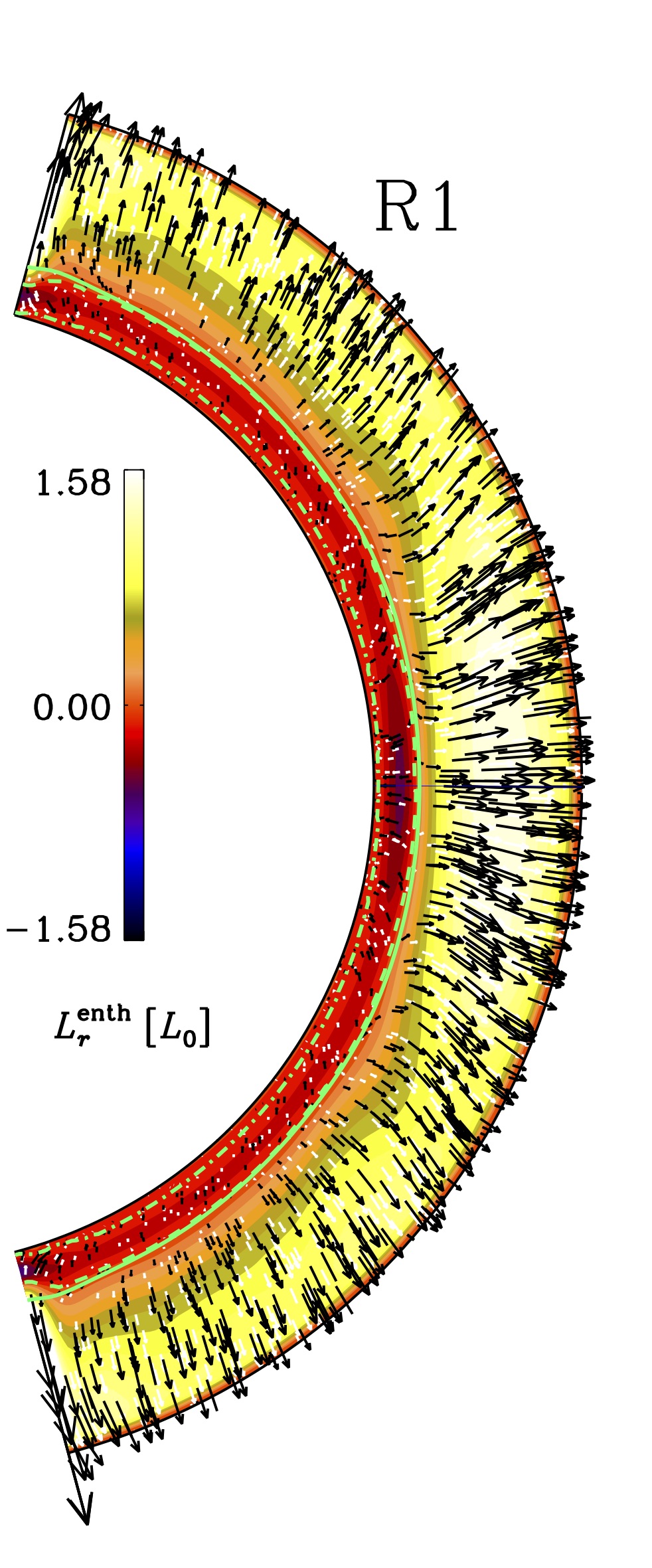
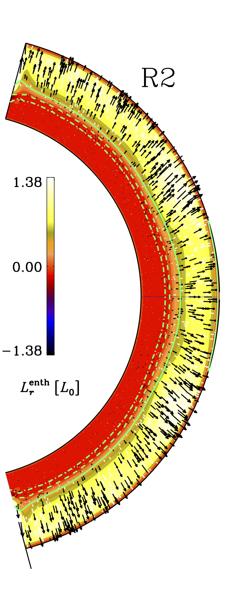
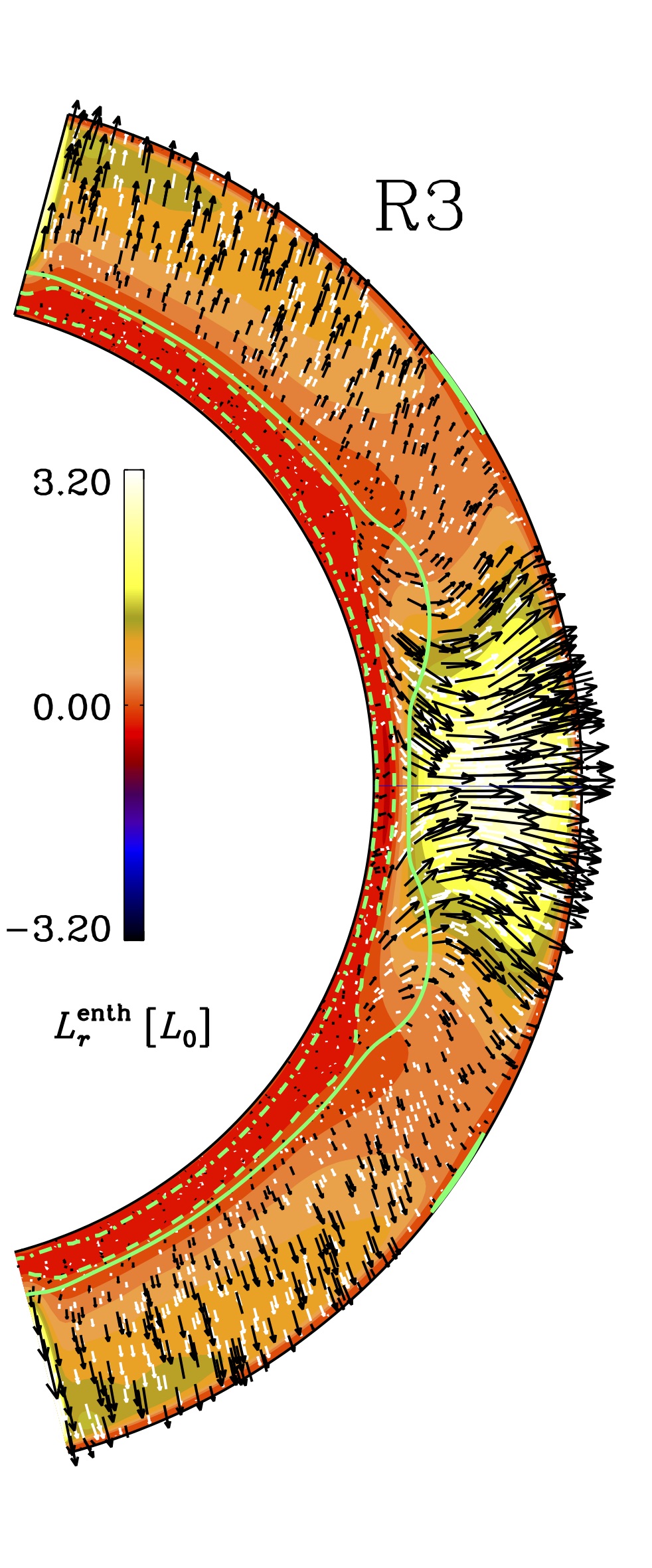
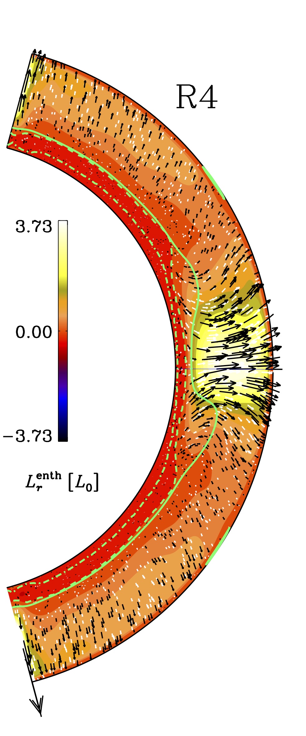
Figure 1: Radial $L^{\rm enth}$ normalized by $L_{0}$. The arrows show the direction of $L^{\rm enth}$. The continuous, dashed and dash-dotted green lines represent, respectively, the bottom boundaries of BZ, DZ and OZ.

We define the convection zone according to the revised structure proposed by Käpylä et al. (2019), and indicate the bottom of the different layers in Figures 1 and 2 and Figure 6 in Appendix A. The radial enthalpy flux is defined as $F^{\rm enth}_{r}=\overline{c_{p}\left(\rho{\bm{u}}_{r}\right)^{\prime}T}$. The bottom of the buoyancy zone (BZ), in which the radial enthalpy flux is greater than zero, $F_{r}^{\rm enth}>0$, and the radial entropy gradient is negative, $\partial_{r}s<0$, is indicated with a continuous green line; we note that our BZ would be the convection zone if defined based on the Schwarzchild criterion. We denote the bottom of the Deardorff layer (DZ), in which $F_{r}^{\rm enth}>0$ and $\partial_{r}s>0$, by a dashed line, and the bottom of the overshoot zone (OZ), for which $F_{r}^{\rm enth}<0$ and $\partial_{r}s>0$, with a dash–dotted line. What we denote as the convection zone is the combination of the BZ and DZ, where enthalpy flux is positive, but entropy gradient can be also positive, meaning that the DZ part of our convection zone is sub–adiabatic. In the radiative zone (RZ), $F_{r}^{\rm enth}\approx 0$ and $\partial_{r}s>0$. The values averaged over latitude and longitude for the depth of the layers are also shown in Table 1. We quote two Coriolis numbers for each simulation. The first one is obtained from Equation (9); the second one, denoted as ${\rm Co}_{\rm rev}$ in Table 1, takes into consideration the wavenumber of the revised convection zone (BZ and DZ), therefore we use $k_{f{\rm rev}}=2\pi/\left(R-r_{\rm DZ}\right)$ (see, also, Käpylä et al. 2019), where $r_{\rm DZ}$ is the latitudinally averaged radius of the Deardorff layer, reported in Table 1.

Run R1 has the deepest BZ of all runs, a very thin DZ and a considerable OZ. A thin RZ develops at the bottom. Run R2 has the thinnest convection zone of all runs. Also the OZ is thin, hence the run develops a very thick RZ. In Runs R1 and R2 the thickness of the layers does not change considerably as function of latitude, except for a slight tendency of the DZ of becoming thicker near the equatorial region for Run R2. For Run R3 the convection zone structure at higher latitudes again resembles the one of Run R1. In the equatorial region, however, the convection zone becomes very deep. Close to the tangent cylinder the BZ becomes considerably shallower, and the DZ developes a ”bulge” in that region. Run R4 also exhibits a convection zone structure that varies strongly with latitude, and closely resembles the one seen in Run R3. Also a hemispheric asymmetry develops in Run R4: the DZ ”bulge” is larger and the BZ is deeper in the lower hemisphere than in the upper one.

3.1.1 Enthalpy flux

We inspect the radial enthalpy flux, $F_{r}^{\rm enth}$, by representing the enthalpy luminosity, $L^{\rm enth}=4\pi r^{2}F_{r}^{\rm enth}$, in Figure 1 with black arrows. The enthalpy flux in Run R1 and R2 is isotropic in latitude and rather radial everywhere in the BZ. There is a slight tendency of the flux being enhanced/decreased in the equatorial region for Run R1/R2. A weak negative flux in the equatorial region is present in the OZ for Run R1. A different situation arises for the two more rapidly rotating runs, where the convective transport of energy is stronger at low latitudes. Especially for Run R3, there is a decrease of the enthalpy flux in the regions of the tangent cylinder. A clear equatorial asymmetry is present in $L_{r}^{\rm enth}$ for Run R4. This asymmetry is also reflected in the convection zone structure, as discussed above.

3.1.2 Differential rotation

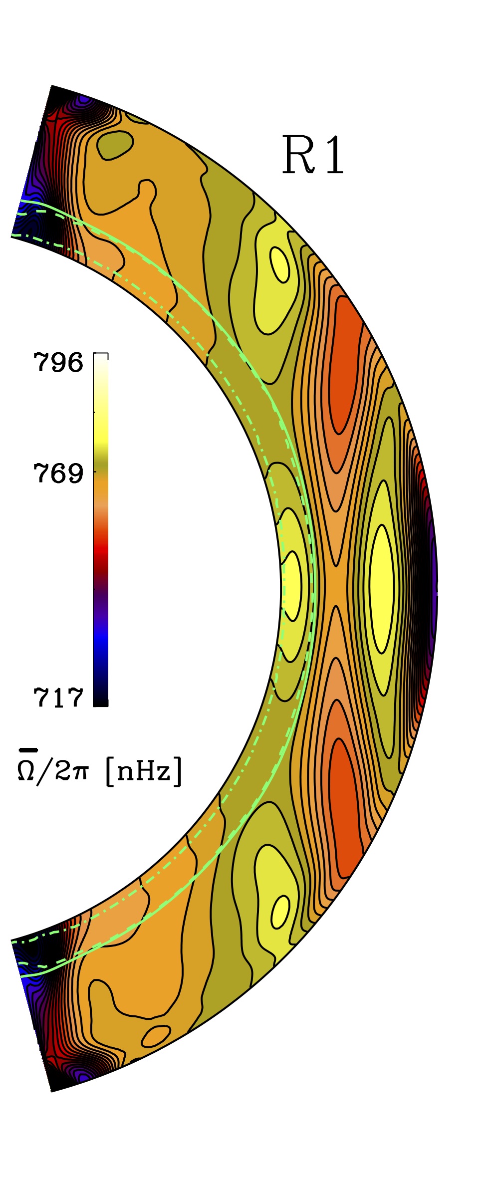
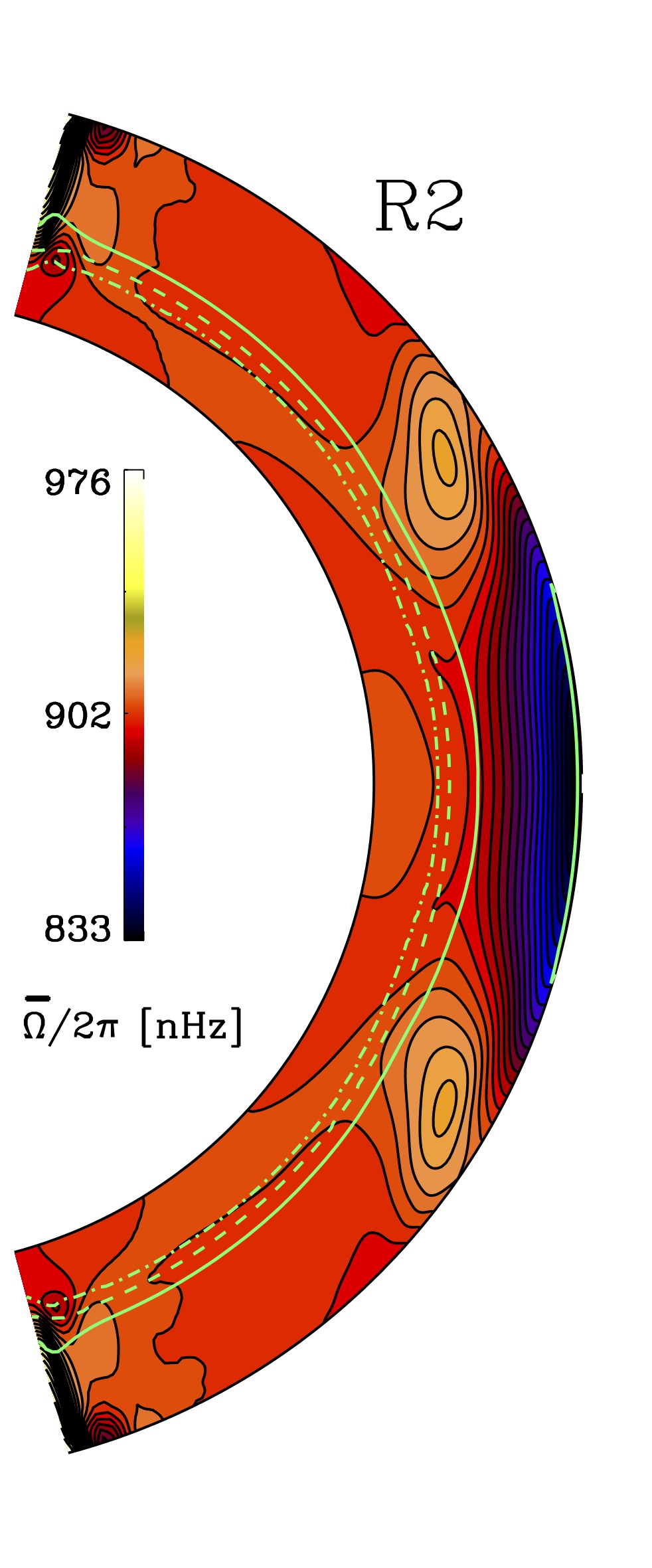
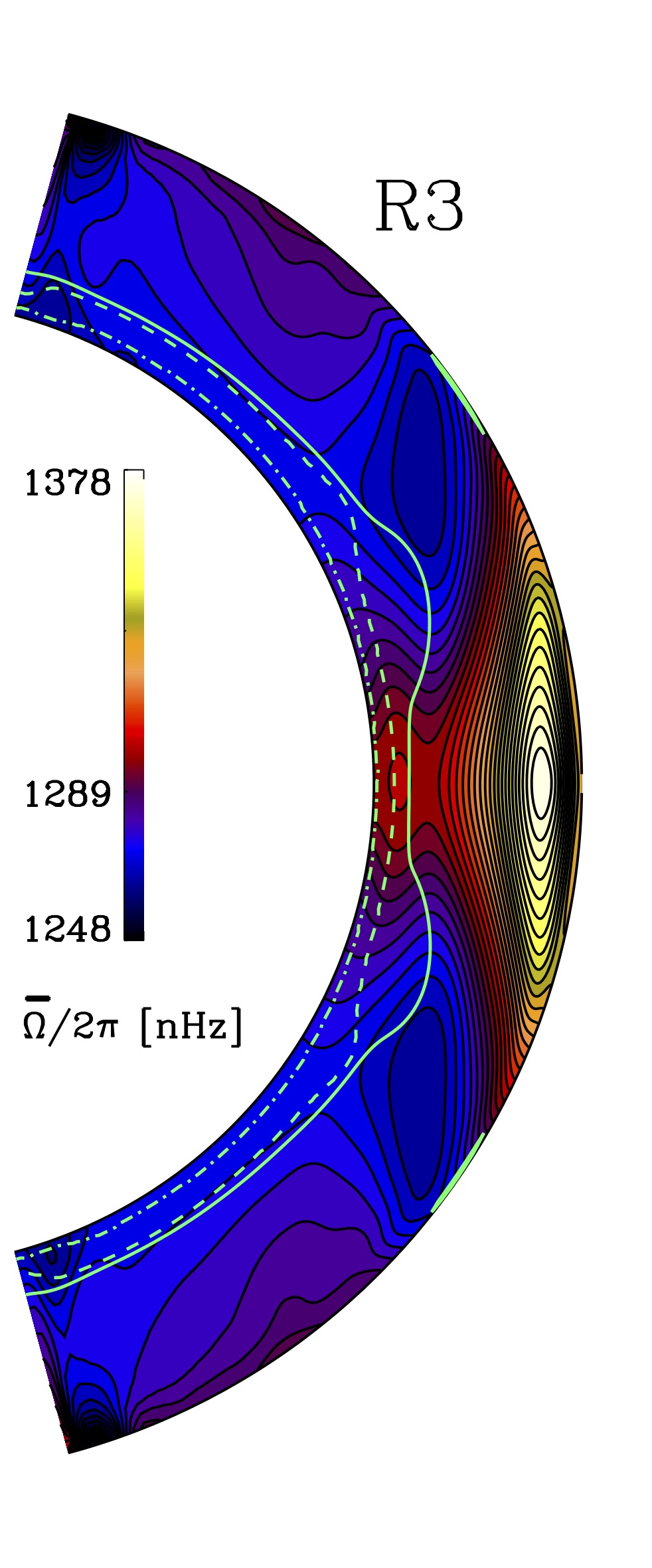
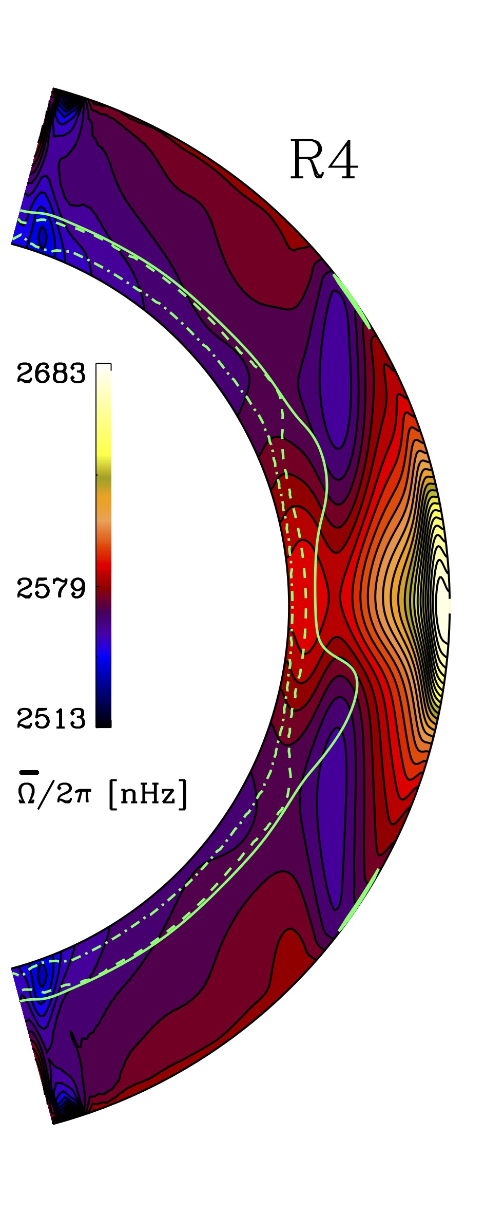
Figure 2: Differential rotation profiles. Continuous, dashed and dash–dotted green lines as in Figure 1.

The last two columns in Table 1 quantify the relative radial and latitudinal differential rotation, defined as:

$$\Delta_{r}=\frac{\Omega_{\rm eq}-\Omega_{\rm bot}}{\Omega_{\rm eq}}\quad{\rm and}\quad\Delta_{\theta}=\frac{\Omega_{\rm eq}-\Omega_{\rm pole}}{\Omega_{\rm eq}}.$$ (10)

Here, $\Omega_{\rm eq}$ is the surface rotation rate at the equator, $\Omega_{\rm bot}$ the equatorial rotation rate at the bottom of the simulation domain and $\Omega_{\rm pole}=\left(\Omega(R,\theta_{0})+\Omega(R,\pi-\theta_{0})\right)/2$. We show the differential rotation profiles in Figure 2 and compare with the corresponding simulations from other works, showing their profiles in Appendix A.

Run R1 corresponds to the simulation with the lowest rotation rate showing an accelerated equator in Viviani et al. (2018), the rotation profile in that case being quite solar–like (see Figure 6, first panel). With an adaptable heat conduction prescription the rotation profile is less solar–like (see, Figure 2, left panel and Table 1): the equatorial acceleration becomes less pronounced, the angular velocity contours are more cylindrical, and additional regions of negative shear appear at mid–latitudes and in the equatorial region close to the surface. Such regions of negative shear at mid–latitudes, in many simulations (e.g., Käpylä et al. 2012; Warnecke et al. 2014), have been identified as responsible for the equatorward propagation of the magnetic field at the surface. In this case, however, we measure weaker relative differential rotation and also the opposite sign in comparison to the results of Viviani et al. (2018), where $\Delta_{r}=0.07$ and $\Delta_{\theta}=0.17$ for Run C3. Hence, our model is even closer to the anti–solar to solar–like differential rotation transition than Run C3 of theirs. Therefore, the contribution of the differential rotation to the large-scale dynamo should be negligible. To assert this, though, a more thorough analysis would be required.

In comparison to Run D in Viviani et al. (2018) (Figure 6, second panel), which had weak values for the relative differential rotation ($\Delta_{r}=0.003$ and $\Delta_{\theta}=0.007$), Run R2 presents stronger DR in absolute value, although with the opposite sign. The rotation profile is anti–solar with a retrograde flow at the equator. At mid–latitudes, a region of accelerated flow develops and the isorotation contours here and at higher latitudes are radially inclined. In the thick RZ the rotation does not vary much in latitude and depth.

The rotation profile of Run R3 (Figure 2) is very similar to the one from its wedge counterpart shown in Figure 6, third panel. It is solar–like, showing an accelerated equator, and has a rather weak relative differential rotation in terms of $\Delta_{r}$ and $\Delta_{\theta}$. The minimum at mid–latitudes is present, and its location corresponds to the sub-adiabatic region at the top boundary, which is probably numerical in nature. A near–surface shear layer, with a negative radial gradient, is present from mid to low latitudes.

The rotation rate of Run R4 corresponds to Run H in Viviani et al. (2018), while its Coriolis number is close to Run G^a in the same study, see also the last two panels in Figure 6. Hence, the usage of the Kramers opacity law produces higher convective velocities and, therefore, smaller ${\rm Co}$. The values for $\Delta_{r}$ and $\Delta_{\theta}$ coincide with the ones from G^a. The rotation profile, shown in Figure 2, rightmost panel, closely resembles that of Run H, with a deep minimum at mid–latitudes.

3.2 Dynamo solutions

Run	E${}_{\rm mag,tot}^{\rm dec}$	E${}_{0}^{\rm dec}$	E${}_{1}^{\rm dec}$	E${}_{2}^{\rm dec}$	E${}_{3}^{\rm dec}$	E${}_{4}^{\rm dec}$	E${}_{5}^{\rm dec}$	E${}_{l,m>5}^{\rm dec}$	$\tau_{\rm cyc}$[yr]
R1	1.4(-2)	4.9(-3)	1.6(-3)	8.2(-4)	7.5(-4)	8.0(-4)	8.5(-4)	4.5(-3)	$1.8_{\rm(m=0)}$
R2	1.5(-2)	9.9(-3)	3.7(-4)	3.9(-4)	4.2(-4)	4.1(-4)	4.8(-4)	2.9(-3)	$1.7_{\rm(m=0)}$
R3	1.8(-2)	5.4(-3)	8.2(-3)	1.2(-3)	7.5(-4)	5.2(-4)	4.4(-4)	1.0(-3)	$3.3_{\rm(m=0)}$
R4	5.0(-2)	1.2(-2)	2.6(-2)	3.4(-3)	1.7(-3)	1.2(-3)	1.0(-3)	4.2(-3)	$2.8_{\rm(m=1)}$

Table 2: Magnetic energy from the decomposition in the first 11 spherical harmonics ($0\leq l,m\leq 10$) of the near-surface ($r=0.98R$) radial magnetic field. The labels E${}_{m}^{\rm dec}$ indicate the energy in the corresponding $m$ mode, in units of $10^{5}\leavevmode\nobreak\ {\rm J\leavevmode\nobreak\ m^{-3}}$. We define $0\leq l,m\leq 5$ the large–scale field. The numbers in parenthesis represent the power of ten. Last column indicates the characteristic time of the dynamo, calculated on the dominant mode, indicated in the subscript.

All the presented runs develop large–scale dynamo (LSD) action, and thereby sustain a magnetic field. The magnetic Reynolds numbers, however, are too low to allow for small–scale dynamo action (SSD). Our dynamo solutions, therefore, exhibit magnetic fields on the largest scales, but also a strong fluctuating component, that is generated by tangling of the LSD–generated magnetic field by the turbulent motions rather than from an SSD. We present the results of the decomposition of the magnetic field in the first 11 spherical harmonics ($0\leq l,m\leq 10$) in Table 2. The decomposition was performed on the radial magnetic field component near the surface of the simulation ($r=0.98R$). For each of the runs, we calculate the characteristic time of variation of the magnetic field, $\tau_{\rm cyc}$, from the time evolution of the dominant dynamo mode. The results are shown in Table 2, last column, and the mode from which $\tau_{\rm cyc}$ is calculated is indicated as a subscript. As described in Viviani et al. (2018), these cycles are at most quasi–periodic, hence Fourier analysis is not suitable here. Instead, we use a syntactic method, which means that we count how many times the dominant mode of the magnetic field peaks above its mean value, and $\tau_{\rm cyc}$ is obtained by dividing the length of the full time span of measurement by the number of peak times.

Run R1 and R2 have a dominant axisymmetric large–scale magnetic field, but also a significant contribution from the small–scale field ($l,m>5$). The energy in the first non–axisymmetric large–scale mode is less than in the mode $m=0$. This is opposite to the case in Viviani et al. (2018), where simulations with the same rotation rates, but a fixed heat conduction profile, were showing a substantial $m=1$ component. Run R3 is in a regime where the axisymmetric and the first non–axisymmetric mode have comparable strengths, hence we characterize this run as being non-axisymmetric. R3, in fact, shows a weak azimuthal dynamo wave (ADW, see, also 3.2.2). For calculating $\tau_{\rm cyc}$, however, we follow the same convention as in Viviani et al. (2018) for runs in this regime, and use $m=0$ to obtain it. Run R4 has a strong $m=1$ component, which is reflected by the presence of the ADW in Figure 5, lower panel.

3.2.1 Axisymmetric magnetic field

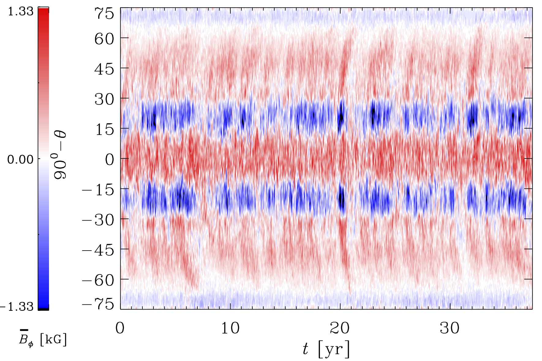
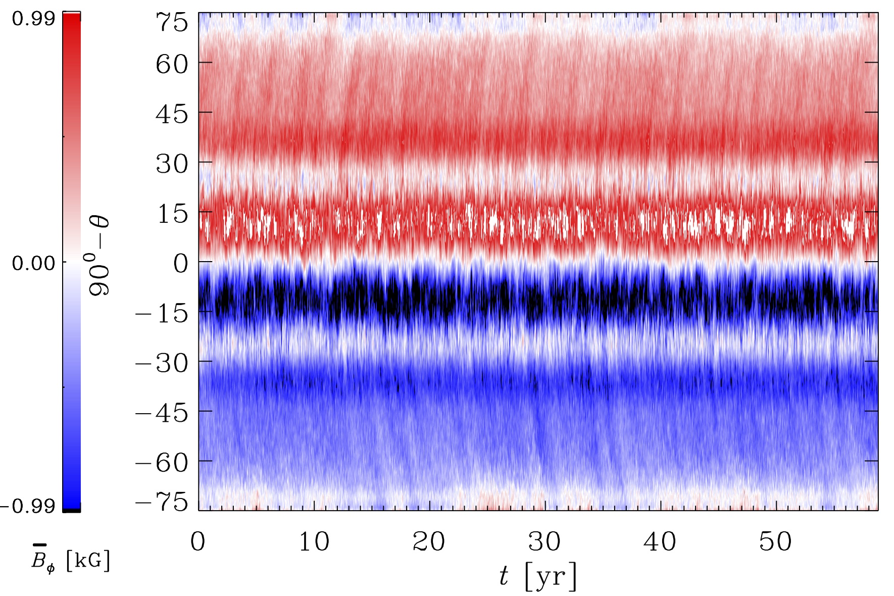
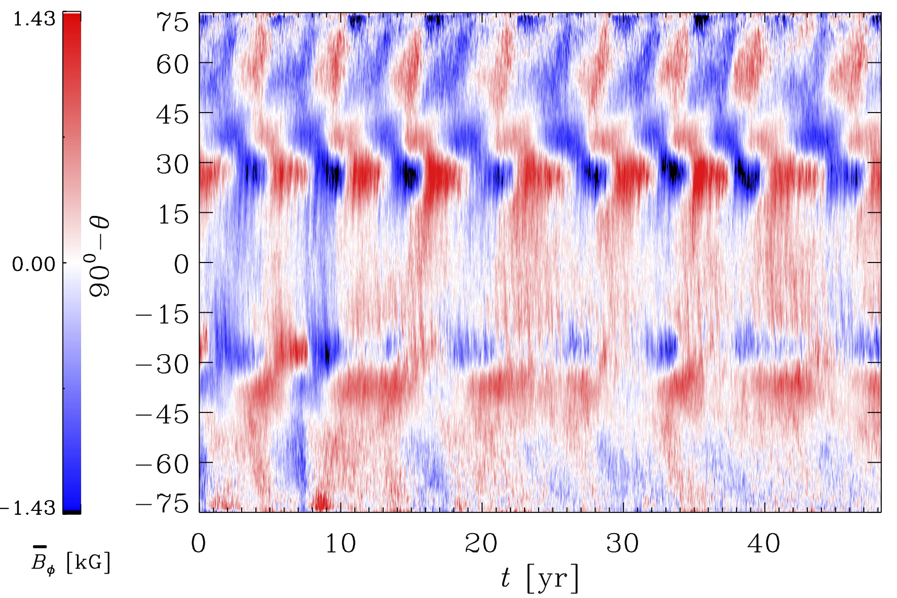
Figure 3: Azimuthal magnetic field at $r=0.98R$ for Run R1 and Run R3.

We show the azimuthally averaged longitudinal magnetic field near the surface as a function of time (the so-called butterfly diagram) in Figure 3. Run R1 is characterized by equatorially symmetric magnetic field, with non–migrating negative polarities at low latitudes and poleward migrating positive field at higher latitudes. A stationary negative field is present at all times close to the latitudinal boundary. A similar, oscillatory dynamo solution was reported and analysed in detail in Viviani et al. (2019). There it was concluded that two dynamo modes were competing in the model, a stationary and an oscillatory one, the latter with polarity reversals. This dynamo was concluded to be driven mostly by turbulent effects, as the differential rotation was found weak in the model. Run R1 appears to be another incarnation of such a dynamo in the transition regime from solar–like to anti–solar differential rotation.

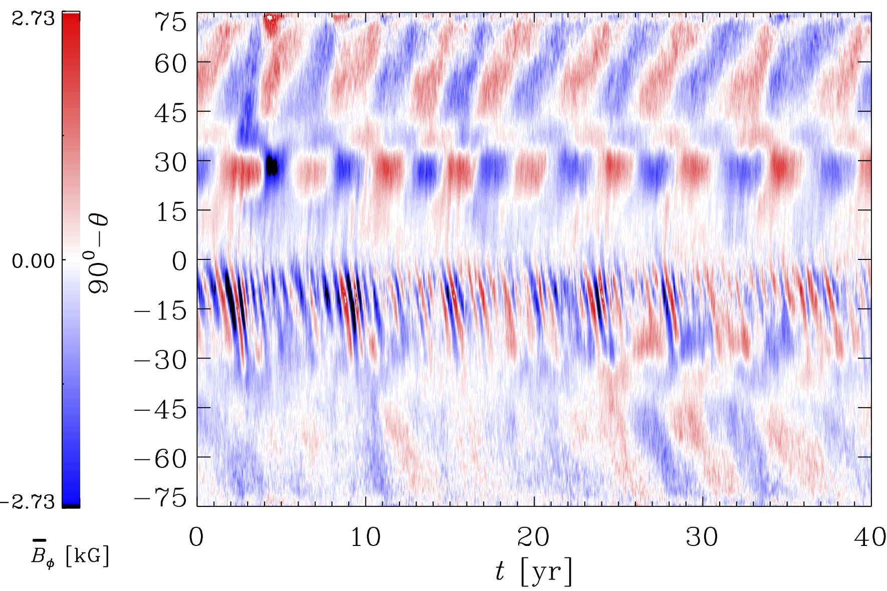
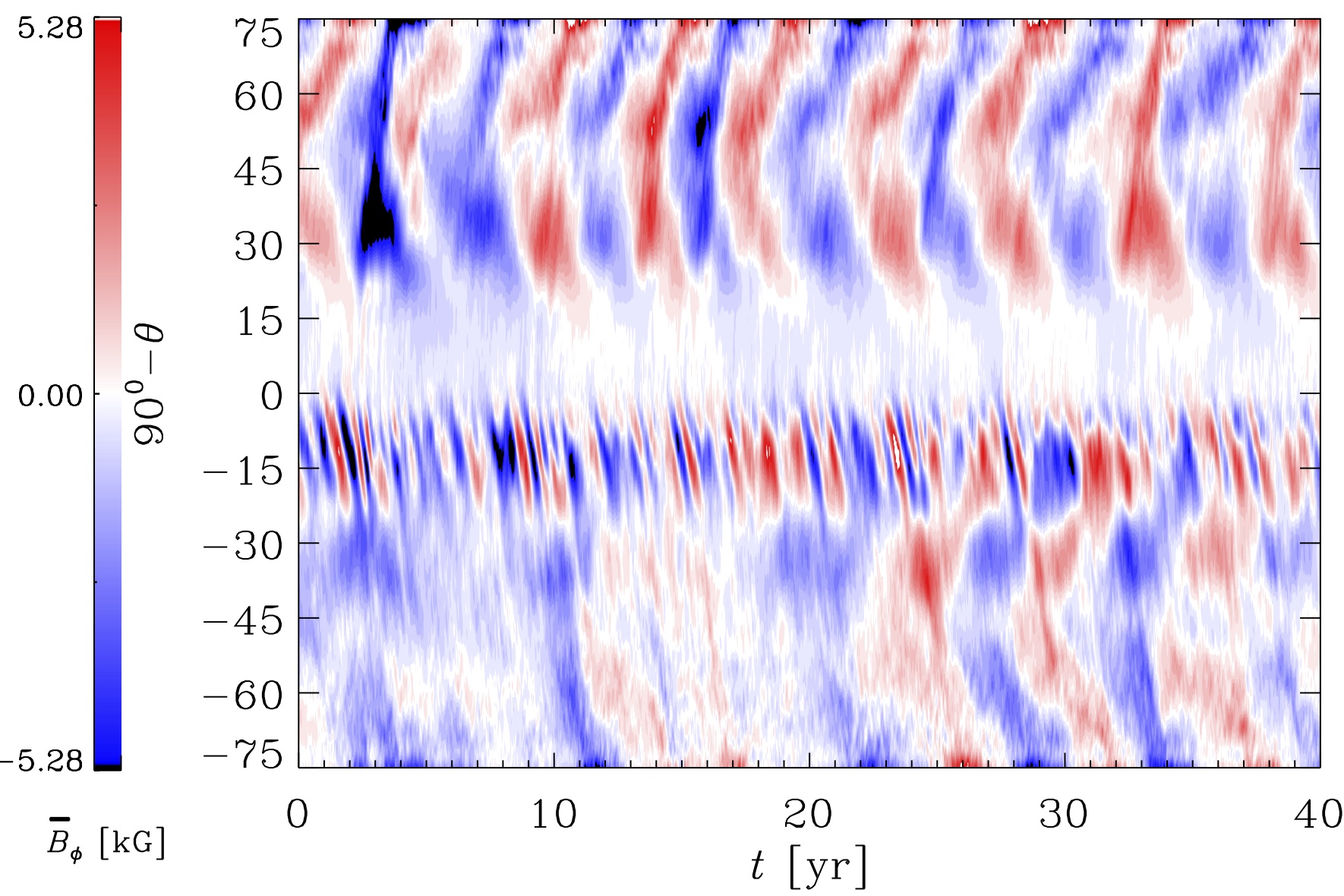
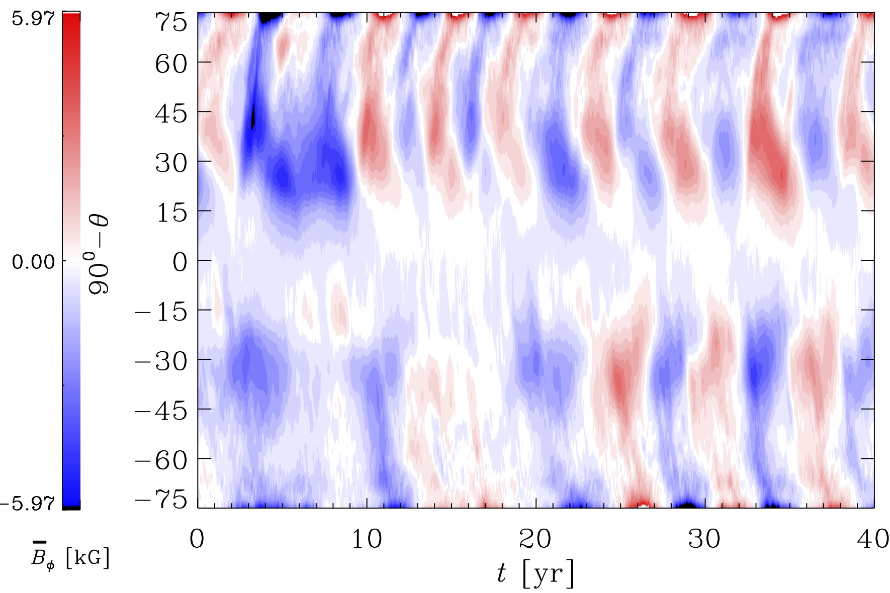
Figure 4: Azimuthal magnetic field for Run R4 at different depths: $r=0.98R$, $r=0.86R$ and $r=0.75R$.

The longitudinally averaged $B_{\phi}$ in Run R2 is dipolar (equatorially antisymmetric) at the surface. The polarity is positive in the upper hemisphere and there are no signs of polarity reversals, if the weak ones at the latitudinal boundaries are not counted for. Also, no equatorward migration can be seen, albeit there is again a tendency for a weak poleward migration with a very high frequency.

Run R3 exhibits equatorial propagation of the azimuthal magnetic field, and the pattern in the butterfly diagram (lowest panel in Fig. 3) is very similar to that of Run MHD2 in Käpylä et al. (2019), also showing a similar periodicity of $\sim 2\leavevmode\nobreak\ {\rm yr}$. In contrast to Run MHD2, the solution shows a pronounced hemispheric asymmetry, with a regular cycle in the upper hemisphere and an irregular periodicity in the lower one. The latter cycle seems to be longer than the one in the upper hemisphere.

In Fig. 4 we show butterfly diagrams at three different depths for Run R4. At the surface, it shows two dynamo modes: a high–frequency one in the lower hemisphere and a lower–frequency one, with a periodicity similar to Run R3, in the upper hemisphere. As we go deeper down to the convection zone, the high–frequency mode disappears, and we can trace its origin to the depth of $0.80\leq r\leq 0.85$, therefore to the bottom of the BZ. The lower–frequency mode, however, persists until the OZ, and therefore we infer that it is generated there. The existence of different dynamo modes at different depths has been reported already in other studies (such as Käpylä et al. 2016, 2019).

3.2.2 Non-axisymmetric magnetic field

In Run R3 a weak azimuthal dynamo wave is present. In Figure 5, upper panel, we plot the reconstructed $m=1$ mode at $45^{o}$ above the equator close to the surface as a function of time and longitude. The black–white dashed line represents the pattern of differential rotation at the same latitude. In the absence of a dynamo wave, the magnetic field would follow the propagation speed of this pattern. Instead, in Figure 5, the magnetic field does not fall on the line for most of the time, hence, it has its own motion as a wave, travelling in the prograde direction. Weak ADWs, such as the one seen in the case of Run R3, were found to be typical in simulations that are close to the axi- to non-axisymmetric transition (Viviani et al. 2018). In this study it was observed that, when the energy in the modes $m=0$ and $m=1$ is comparable, the ADW can be affected by the differential rotation, in which case it becomes advected by it for some time intervals (see Figure 5, left panel, $0\leavevmode\nobreak\ {\rm yr}\leq t\leq 15\leavevmode\nobreak\ {\rm yr}$). ADWs were already found in other numerical studies (Käpylä et al. 2013; Cole et al. 2014; Viviani et al. 2018), but their direction was mostly retrograde, in contrast with observational results (see, e.g., Lehtinen et al. 2016).

A stronger prograde ADW is also present in Run R4. The wave does not persist at all times, but there are periods when it disappears. Similar behaviour was also observed, for example, in the temperature maps of the active star II Peg in Lindborg et al. (2011), where a very clearly defined prograde ADW persisted over ten years, but then vanished. Also Lehtinen et al. (2012) and Olspert et al. (2015) reported on ADWs on the young solar analogue star LQ Hya, but these lasted even for a shorter period of time, of about a couple of years. We attribute the change in the ADW direction to the different heat conduction prescription in these runs. Moreover, in Run R3 the ADW can even change direction from prograde to retrograde during some short epochs, most likely related to the stronger influence from the differential rotation. Such a change of direction in the migration of active longitudes has also been observed, e.g. in the study of Korhonen et al. (2004) in the case of the intensively studied single active star FK Coma Berenices.

We calculate the period of the ADW, $P_{\rm ADW}$ as in Viviani et al. (2018), taking the latitudinal and temporal average of the slope of the reconstructed time evolution of the $m=1$ mode. For R3, we obtain $P_{\rm ADW}=-24.5\leavevmode\nobreak\ {\rm yr}$, the minus sign indicating a negative slope, therefore a retrograde direction for the dynamo wave, in contrast with the mostly prograde appearance of the migration in Figure 5, upper panel. As discussed before, the ADW in R3 is chaotic, even changing its direction, and also disappearing, and this causes the average period to be an inaccurate measure. $P_{\rm ADW}=44.9\leavevmode\nobreak\ {\rm yr}$ for Run R4, the positive sign indicating a prograde wave, as expected. From the lower panel of Figure 5, however, we would infer a shorter period $\sim\leavevmode\nobreak\ 30\leavevmode\nobreak\ {\rm yr}$.

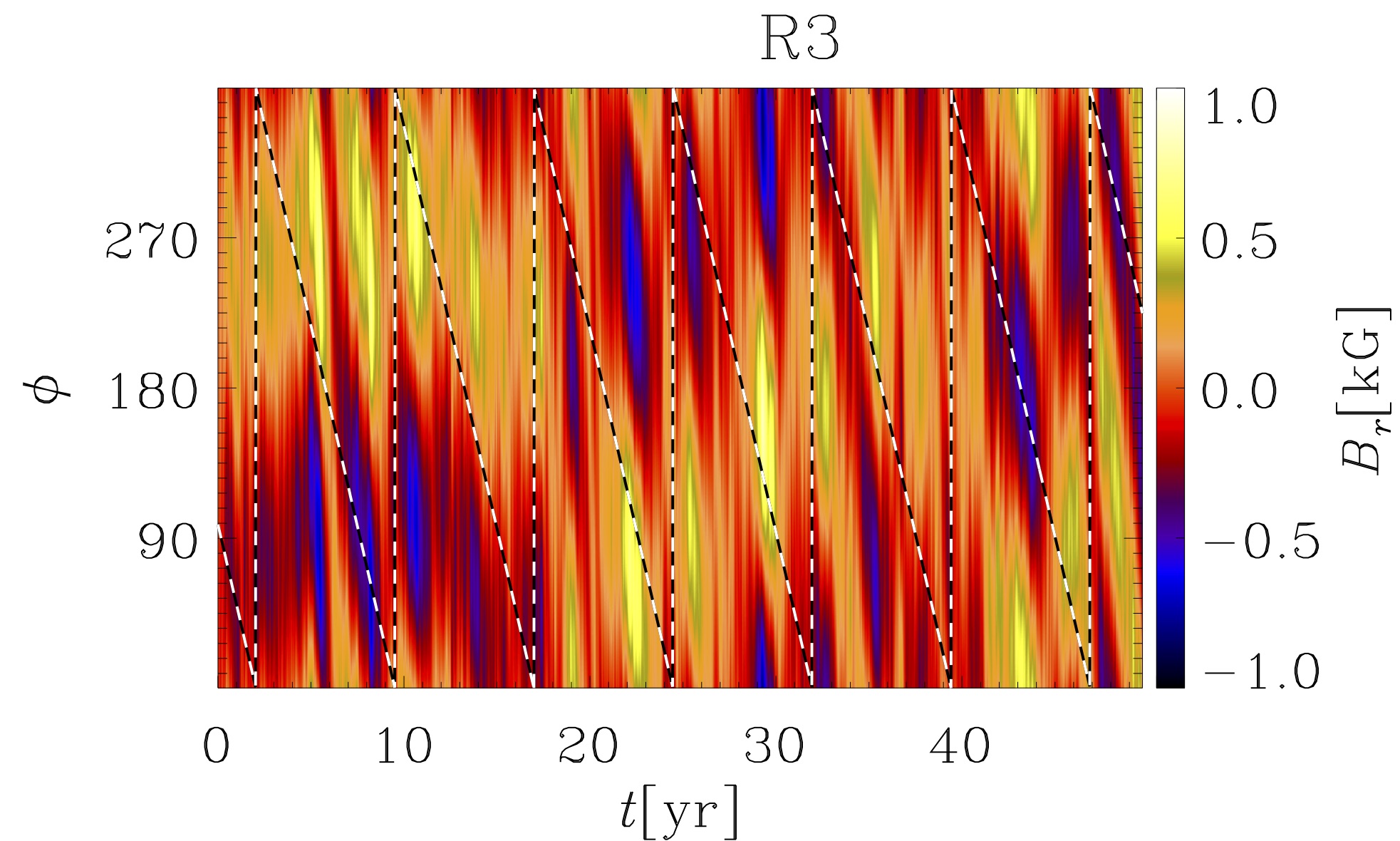
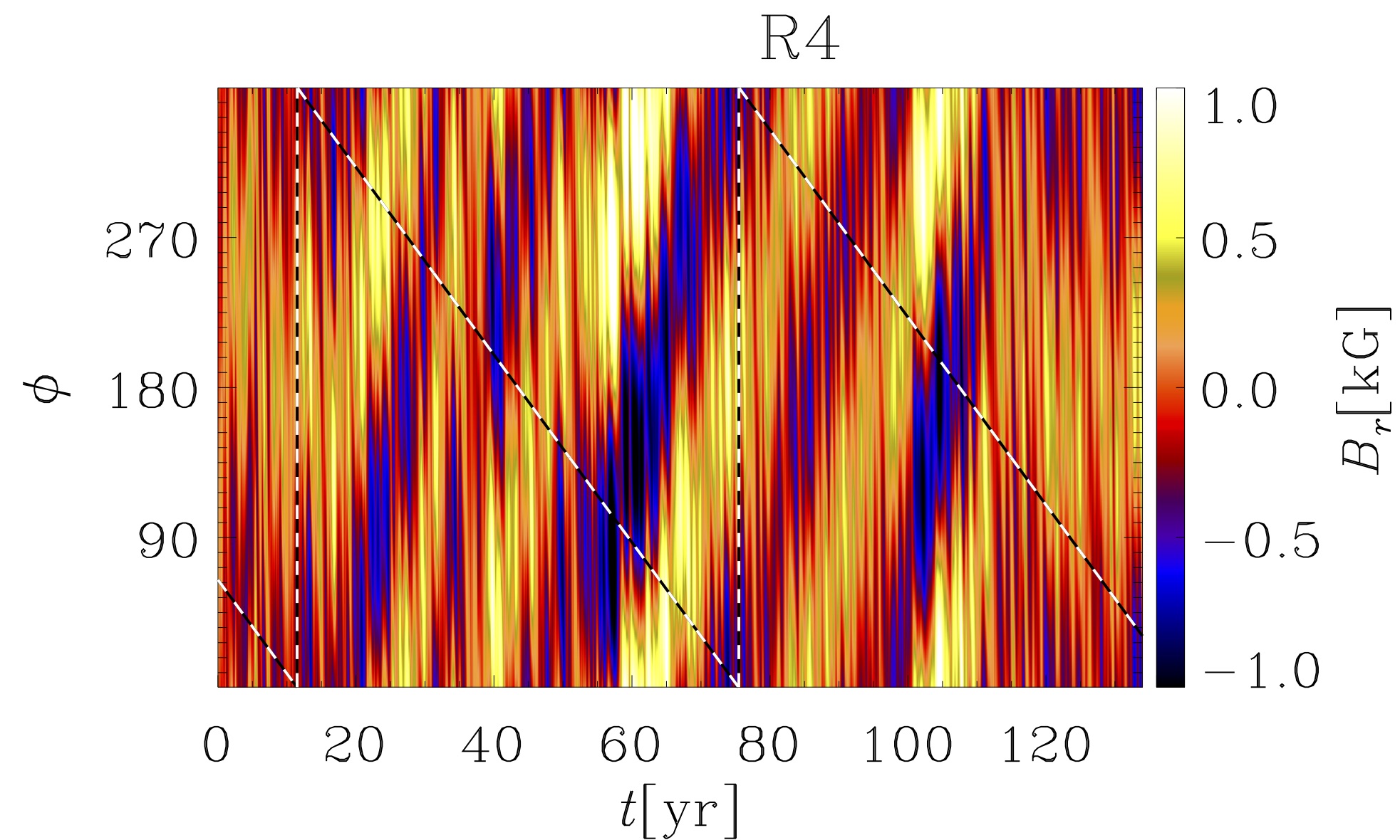
Figure 5: Azimuthal dynamo wave for Runs R3 and R4 as a function of longitude and time, at latitude $\theta=+45^{o}$ and depth $r=0.98R$. The black and white dashed line represents the differential rotation at the same latitude.

4 Conclusions

In this paper we studied the effect of a dynamically adapting heat conduction prescription, based on Kramers opacity law, on semi–global MHD simulations. The main aim was to determine its effect on the two major transitions reported in numerical studies (e.g., Gastine et al. 2014; Viviani et al. 2018). One concerns the rotation profiles, and is the transition from accelerated poles and decelerated equator to a solar–like profile, with faster equator. The other one involves the large–scale magnetic field, and is the transition from an axisymmetric magnetic field, as in the Sun, to a non–axisymmetric one found in more rapid rotators. Previous studies (Viviani et al. 2018) reported these transitions occurring at the same rotation rate, in contrast with the current interpretation of observations. The fact that simulations usually produce anti–solar differential rotation for the solar rotation rate could indicate that the Sun is in a transitional regime (e.g., Käpylä et al. 2014; Metcalfe et al. 2016), or it could also mean that simulations still cannot fully capture the right rotational influence on turbulent convection in the Sun. The study of Lehtinen et al. (2016) reported on the existence of non–axisymmetric structures in stars with varying rotation rates, and hence could determine quite a sharp transition point, in terms of the rotation period, when fields turn from axi– to non–axisymmetric configurations. According to dynamo theory, these two modes can compete, and there can be a transition region, where both dynamo modes co–exist, as is also clearly demonstrated by the models presented in this paper and Viviani et al. (2018). Hence, the observational transition point must be regarded as a lower limit, in terms of the rotation period, for the transition, as it could be that the sensitivity of the current instruments is not high enough to detect the very weak non–axisymmetric components. Since active longitudes have not been detected on the Sun (Pelt et al. 2006), though, these two transitions should not be located at the same, nearly solar, rotation rate.

In runs with slow rotation, the differential rotation profile is significantly affected by the Kramers opacity law and, as a result, solutions with less solar–like characteristics, like an almost rigid body rotation and a minimum at mid–latitudes, develop. The different heat conduction prescription also promotes the formation of a stably stratified layer, rather isotropic in latitude, in the lower quarter of the domain. For faster rotating runs, the rotation profile is solar–like, but still maintains the minimum at mid–latitudes, and a latitudinally changing subadiabatic region forms near the equator. Also, the Coriolis number is lower than in the corresponding cases using fixed profiles for heat conduction, which is most likely the largest contributing factor to push the anti–solar to solar differential rotation transition to an unwanted direction of more rapid rotation rates.

The convective transport is efficient, isotropic and almost radial everywhere in the convective region in models with slow rotation (Runs R1 and R2), while it gets strongly concentrated to the equatorial region in runs with more rapid rotation (Runs R3 and R4). Also, the BZ becomes shallower close to the tangent cylinder in the rapid rotation regime. Moreover, hemispheric asymmetries in the convection zone structure are seen in the run with the fastest rotation (Run R4).

The large–scale magnetic field is axisymmetric in Run R1 and R2, while for Run R3 and Run R4 the first non–axisymetric mode is dynamically more important. Both the fast rotating runs have a hemispherically asymmetric oscillating magnetic field, with a periodicity of $\sim\leavevmode\nobreak\ 2$ years. As in Viviani et al. (2018), the magnetic cycle lengths do not overall depend strongly on the rotation period. The strong magnetic field in all the runs originates from the subadiabatic layer. In Run R4 a high–frequency mode is present in the lower hemisphere. This component is generated at the bottom boundary of the BZ. The co–existence of multiple dynamo modes at different depths of the convection zone is consistent with previous studies (e.g., Käpylä et al. 2016), using prescribed profiles for heat conduction. In this study, the high–frequency mode was generated near the surface, while the low–frequency one in the middle of the CZ.

In the non–axisymmetric runs, ADWs are present: a weak one for Run R3 and a stronger one for Run R4. In both cases, the direction is prograde, in agreement with photometric observations (Lehtinen et al. 2016). In the previous numerical study using a prescribed heat conduction profile (Viviani et al. 2018), we found a preference for retrograde ADWs. The ADWs also show time variations. For Run R3, the ADW is rather weak and the differential rotation can advect it for some time, changing the direction of the wave. This could be caused by the comparable relative energies in the $m=0$ and $m=1$ modes. In Run R4 the stronger ADW disappears at certain times. Such behavior is also what is observed for active stars (e.g., Korhonen et al. 2004; Lindborg et al. 2011; Lehtinen et al. 2012; Olspert et al. 2015), where the active longitudes disappear or have the same velocity as the surface rotation.

In summary, in this study we have shown that both the major transitions related to stellar dynamos are affected by the use of a more physical description of heat conduction in global magneto–convection simulations. The differential rotation profiles undergo a significant change near the anti–solar to solar–like differential rotation transition, but all the runs are still in Taylor–Proudman balance, with almost cylindrical isocontours. For the same rotation rates, the convective velocities are higher, hence Coriolis numbers are lowered, resulting in an anticipated transition to anti–solar differential rotation, in contrast with observations. The transition from axi– to non–axisymmetric magnetic fields is shifted towards higher rotation rates. The direction of the ADW is reverted with respect to previous studies, producing a better agreement with observations.

Appendix A Comparison with rotation profiles in previous works

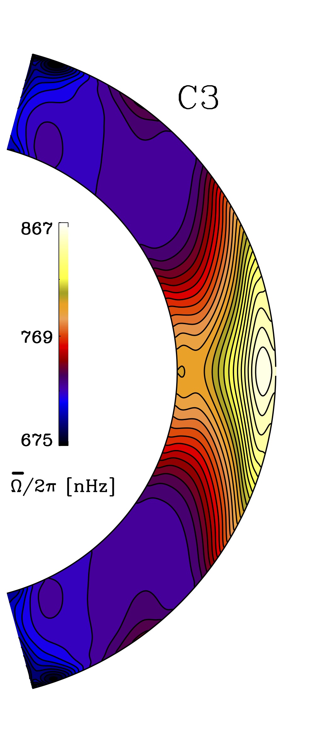
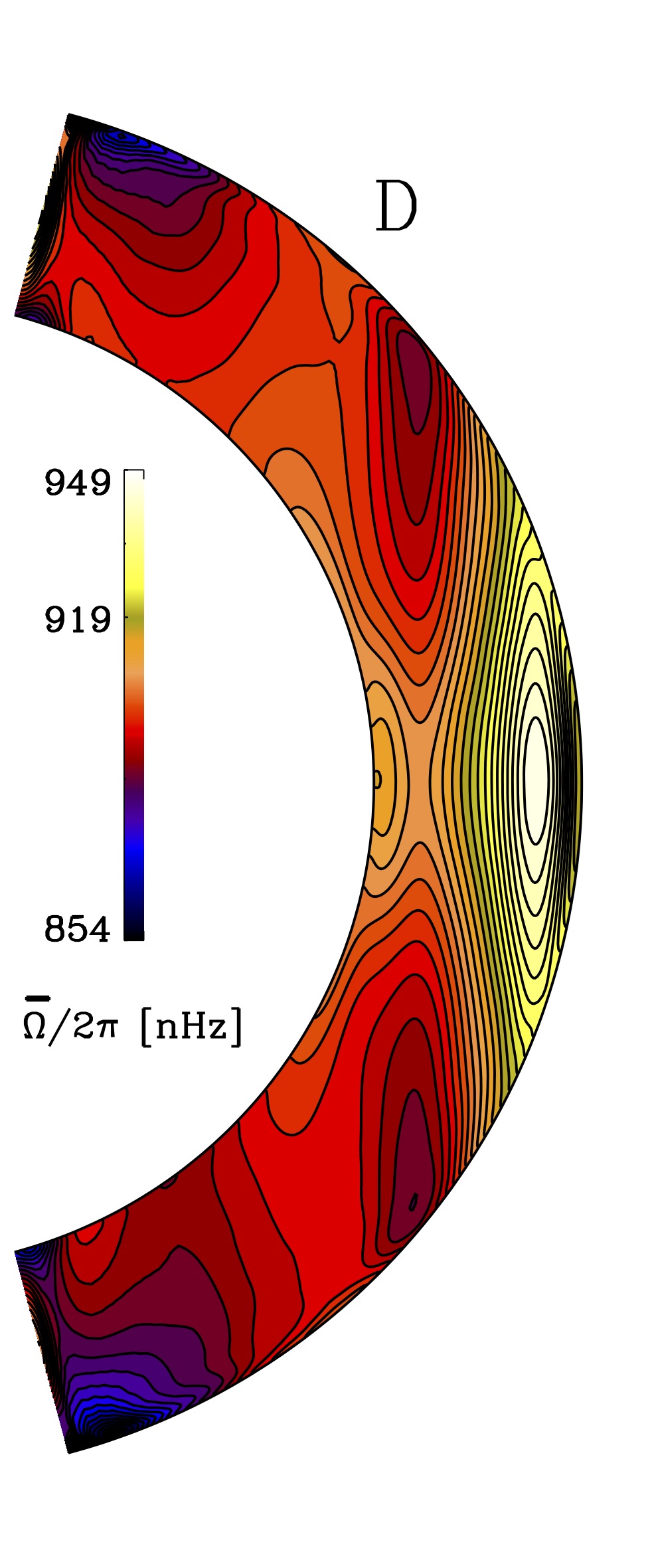
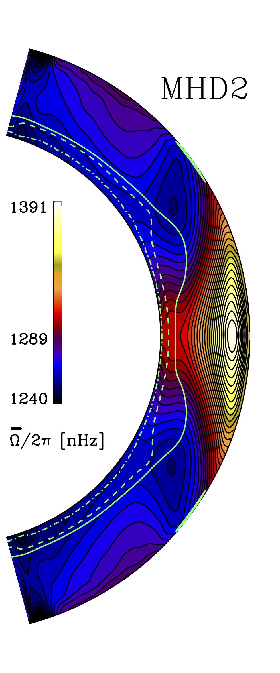
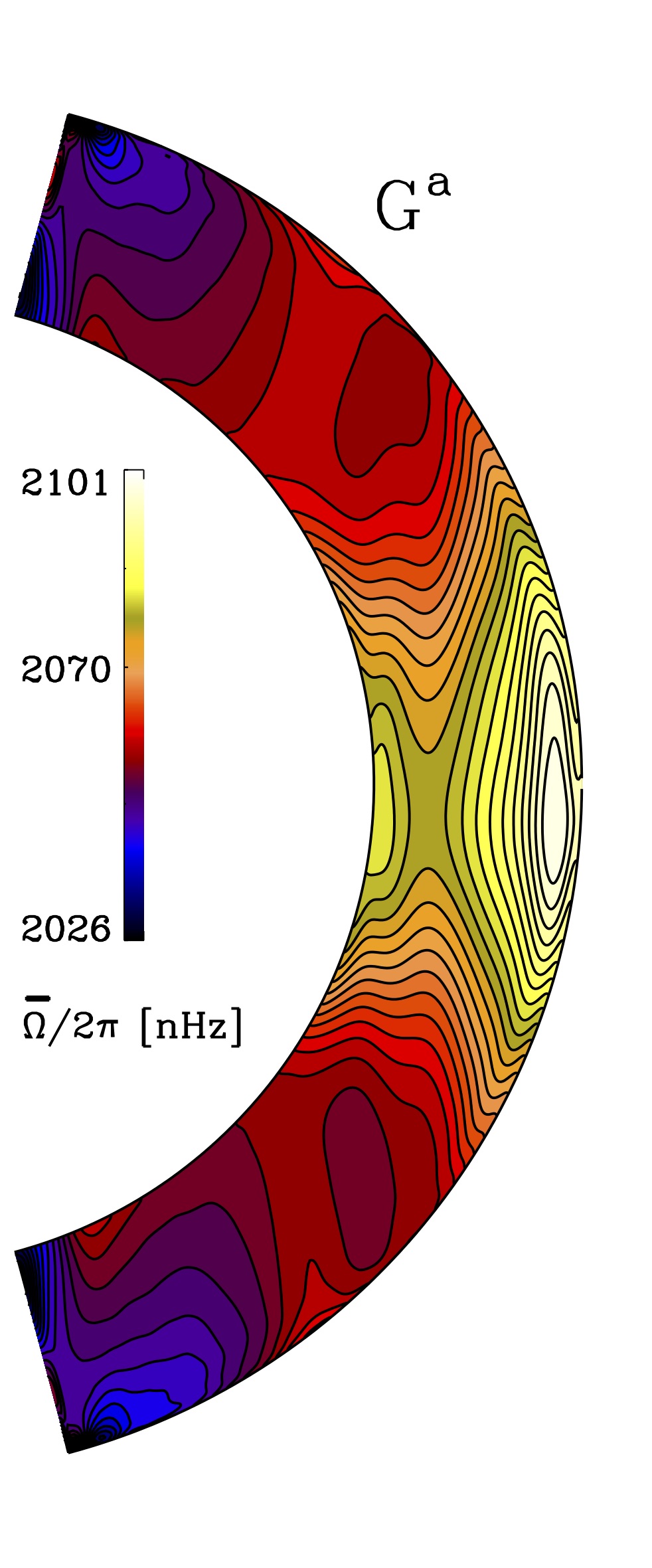
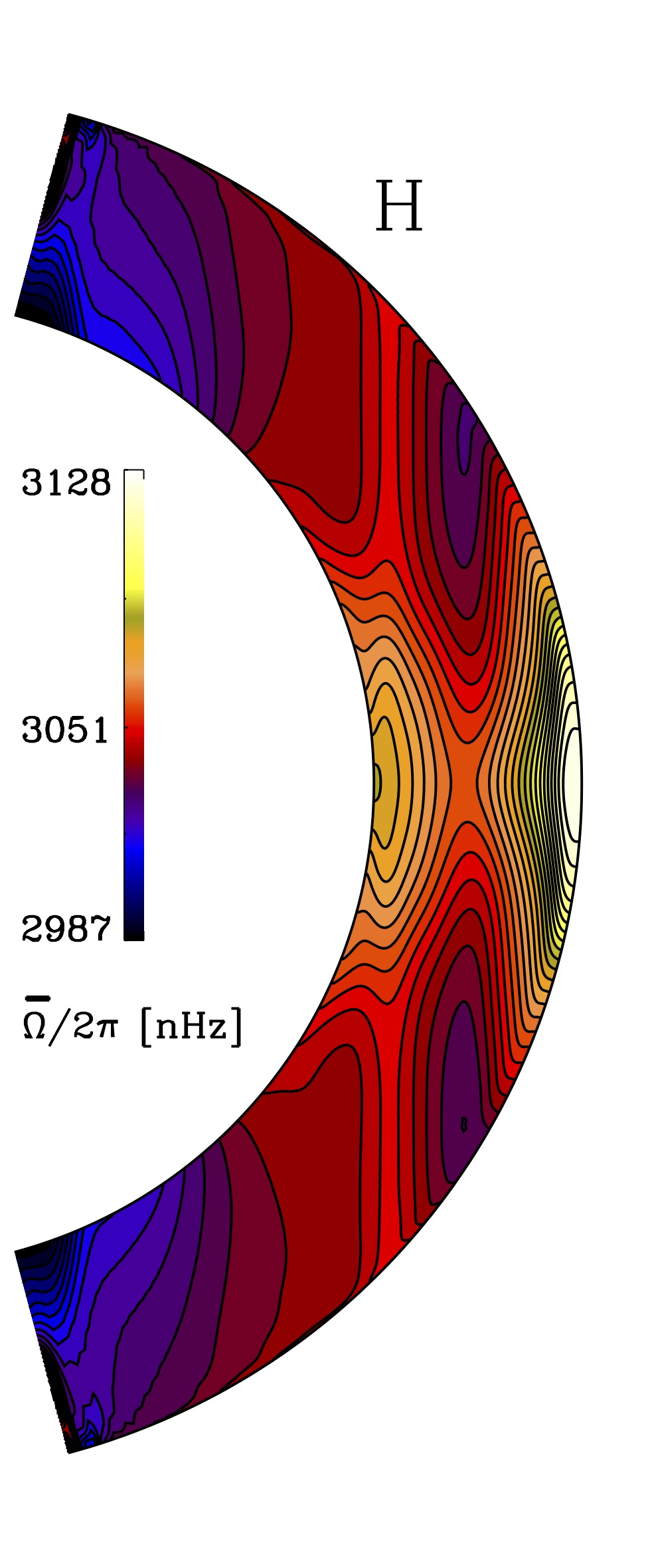
Figure 6: Differential rotation profiles for runs C3, D, G^a, H from Viviani et al. (2018), and MHD2 from Käpylä et al. (2019). The green lines for MHD2 indicate the internal structure as for the simulations in the main text.

We reproduce in Figure 6, for comparison, the differential rotation profiles for the simulations with fixed heat conduction profiles (Runs C3, D, G^a and H) from Viviani et al. (2018), corresponding, respectively, to R1, R2 and R4 (the latter for G^a and H) presented in this paper. We also show again the wedge simulation MHD2 from Käpylä et al. (2019), this time showing both the hemispheres.

The rotational profile of Run D was not presented in the previous publications. An equatorial prograde flow and mid-latitude minima are present, while in its Kramers counterpart, Run R2, the profile is swapped to anti-solar with a decelerated equator and accelerated mid-latitude regions.

References

- Augustson et al. (2015) Augustson, K., Brun, A. S., Miesch, M., & Toomre, J. 2015, ApJ, 809, 149
- Barekat & Brandenburg (2014) Barekat, A. & Brandenburg, A. 2014, A&A, 571, A68
- Berdyugina & Tuominen (1998) Berdyugina, S. V. & Tuominen, I. 1998, A&A, 336, L25
- Böhm-Vitense (1958) Böhm-Vitense, E. 1958, ZAp, 46, 108
- Brandenburg (2016) Brandenburg, A. 2016, ApJ, 832, 6
- Brandenburg et al. (2005) Brandenburg, A., Chan, K. L., Nordlund, Å., & Stein, R. F. 2005, AN, 326, 681
- Browning et al. (2006) Browning, M. K., Miesch, M. S., Brun, A. S., & Toomre, J. 2006, ApJ, 648, L157
- Brun et al. (2011) Brun, A. S., Miesch, M. S., & Toomre, J. 2011, ApJ, 742, 79
- Carrington (1863) Carrington, R. C. 1863, Observations of the spots on the Sun (London), 604
- Chandrasekhar (1961) Chandrasekhar, S. 1961, Hydrodynamic and hydromagnetic stability
- Cole et al. (2014) Cole, E., Käpylä, P. J., Mantere, M. J., & Brandenburg, A. 2014, ApJL, 780, L22
- Deardorff (1961) Deardorff, J. W. 1961, J. Atmosph. Sci., 18, 540
- Deardorff (1966) Deardorff, J. W. 1966, J. Atmosph. Sci., 23, 503
- Gastine et al. (2014) Gastine, T., Yadav, R. K., Morin, J., Reiners, A., & Wicht, J. 2014, MNRAS, 438, L76
- Gizon & Birch (2012) Gizon, L. & Birch, A. C. 2012, PNAS, 109, pp.11896
- Guerrero et al. (2013) Guerrero, G., Smolarkiewicz, P. K., Kosovichev, A. G., & Mansour, N. N. 2013, ApJ, 779, 176
- Hanasoge et al. (2012) Hanasoge, S. M., Duvall, T. L., & Sreenivasan, K. R. 2012, Proc. Natl. Acad. Sci., 109, 11928
- Hotta (2017) Hotta, H. 2017, ApJ, 843, 52
- Hotta et al. (2015) Hotta, H., Rempel, M., & Yokoyama, T. 2015, ApJ, 803, 42
- Jetsu (1996) Jetsu, L. 1996, A&A, 314, 153
- Käpylä et al. (2016) Käpylä, M. J., Käpylä, P. J., Olspert, N., et al. 2016, A&A, 589, A56
- Käpylä (2019) Käpylä, P. J. 2019, A&A, 631, A122
- Käpylä et al. (2020) Käpylä, P. J., Gent, F. A., Olspert, N., Käpylä, M. J., & Brandenburg, A. 2020, GAFD, 114, 8
- Käpylä et al. (2014) Käpylä, P. J., Käpylä, M. J., & Brandenburg, A. 2014, A&A, 570, A43
- Käpylä et al. (2012) Käpylä, P. J., Mantere, M. J., & Brandenburg, A. 2012, ApJ, 755, L22
- Käpylä et al. (2013) Käpylä, P. J., Mantere, M. J., Cole, E., Warnecke, J., & Brandenburg, A. 2013, ApJ, 778, 41
- Käpylä et al. (2017) Käpylä, P. J., Rheinhardt, M., Brandenburg, A., et al. 2017, ApJ, 845, L23
- Käpylä et al. (2019) Käpylä, P. J., Viviani, M., Käpylä, M. J., Brandenburg, A., & Spada, F. 2019, GAFD, 133, p.149
- Karak et al. (2015) Karak, B. B., Käpylä, P. J., Käpylä, M. J., et al. 2015, A&A, 576, A26
- Karak et al. (2018) Karak, B. B., Miesch, M., & Bekki, Y. 2018, Physics of Fluids, 30, 046602
- Kazantsev (1968) Kazantsev, A. P. 1968, Soviet Journal of Experimental and Theoretical Physics, 26, 1031
- Kitchatinov & Rüdiger (1995) Kitchatinov, L. L. & Rüdiger, G. 1995, A&A, 299, 446
- Korhonen et al. (2004) Korhonen, H., Berdyugina, S. V., & Tuominen, I. 2004, Astronomische Nachrichten, 325, 402
- Korre et al. (2017) Korre, L., Brummell, N., & Garaud, P. 2017, arXiv:1704.00817
- Lehtinen et al. (2012) Lehtinen, J., Jetsu, L., Hackman, T., Kajatkari, P., & Henry, G. W. 2012, A&A, 542, A38
- Lehtinen et al. (2016) Lehtinen, J., Jetsu, L., Hackman, T., Kajatkari, P., & Henry, G. W. 2016, A&A, 588, A38
- Lindborg et al. (2011) Lindborg, M., Korpi, M. J., Hackman, T., et al. 2011, A&A, 526, A44
- Metcalfe et al. (2016) Metcalfe, T. S., Egeland, R., & van Saders, J. 2016, ApJ, 826, L2
- Nordlund et al. (2009) Nordlund, Å., Stein, R. F., & Asplund, M. 2009, Living Reviews in Solar Physics, 6, 2
- Olspert et al. (2015) Olspert, N., Käpylä, M. J., Pelt, J., et al. 2015, A&A, 577, A120
- O’Mara et al. (2016) O’Mara, B., Miesch, M. S., Featherstone, N. A., & Augustson, K. C. 2016, Advances in Space Research, 58, 1475
- Pelt et al. (2006) Pelt, J., Brooke, J. M., Korpi, M. J., & Tuominen, I. 2006, A&A, 460, 875
- Rast et al. (2008) Rast, M. P., Ortiz, A., & Meisner, R. W. 2008, ApJ, 673, 1209
- Rempel (2005) Rempel, M. 2005, ApJ, 622, 1320
- Rincon et al. (2017) Rincon, F., Roudier, T., Schekochihin, A. A., & Rieutord, M. 2017, A&A, 599, A69
- Rüdiger (1989) Rüdiger, G. 1989, Differential Rotation and Stellar Convection. Sun and Solar-type Stars (Berlin: Akademie Verlag)
- Scheiner (1630) Scheiner, C. 1630, Rosa Ursina
- Schou et al. (1998) Schou, J., Antia, H. M., Basu, S., et al. 1998, ApJ, 505, 390
- See et al. (2016) See, V., Jardine, M., Vidotto, A. A., et al. 2016, MNRAS, 462, 4442
- Spruit (1997) Spruit, H. 1997, Mem. Soc. Astron. Italiana, 68, 397
- Tuominen et al. (2002) Tuominen, I., Berdyugina, S. V., & Korpi, M. J. 2002, Astronomische Nachrichten, 323, 367
- Vitense (1953) Vitense, E. 1953, ZAp, 32, 135
- Viviani et al. (2019) Viviani, M., Käpylä, M. J., Warnecke, J., Käpylä, P. J., & Rheinhardt, M. 2019, arXiv e-prints, arXiv:1902.04019
- Viviani et al. (2018) Viviani, M., Warnecke, J., Käpylä, M. J., et al. 2018, A&A, 616, A160
- Warnecke et al. (2014) Warnecke, J., Käpylä, P. J., Käpylä, M. J., & Brandenburg, A. 2014, ApJ, 796, L12