Quantum correlations and quantum-memory-assisted entropic uncertainty relation in a quantum dot system

Abstract

The uncertainty principle is one of the comprehensive and fundamental concept in quantum theory. This principle states that it is not possible to simultaneously measure two incompatible observatories with high accuracy. Uncertainty principle has been formulated in various form. The most famous type of uncertainty relation is expressed based on the standard deviation of observables. In quantum information theory the uncertainty principle can be formulated using Shannon and von Neumann entropy. Entropic uncertainty relation in the presence of quantum memory is one of the most useful entropic uncertainty relations. Due to their importance and scalability, solid state systems have received considerable attention nowadays. In this work we will consider a quantum dot system as a solid state system. We will study the quantum correlation and quantum memory assisted entropic uncertainty in this typ of system. We will show that the temperature in of quantum dot system can affect the quantum correlation and entropic uncertainty bound. It will be observed that the entropic uncertainty bound decreases with decreasing temperature and quantum correlations decreases with increasing the temperature.

Keywords: quantum coherence, entropic uncertainty relation, Heisenberg XYZ model

PACS 03.67.-a, 03.65.Ta, 03.67.Hk, 75.10.Pq

1 Introduction

According to the fundamental role of quantum correlations in quantum information theory, this subject has been extensively studied in recent years [1, 2, 3, 4, 5, 6, 7, 8]. It makes a variety of applications possible in quantum information theory such as quantum teleportation [6, 9], quantum cryptography [10], quantum dense coding [11], quantum computing [12, 13, 14] and quantum communication [15, 16]. In previous decades, it has been thought that the only correlation in quantum information theory is entanglement. Hence, different criteria were introduced to measure the entanglement, including concurrence [2], von Neumann entropy, negativity and logarithmic negativity [17, 18], entanglement cost [19, 20], entanglement of formation [2], squashed entanglement [21], robustness of entanglement for bipartite entanglement [22], tangle [23, 24], relative entropy [25], generalized concurrence [26, 27, 28, 29], geometric measures [30, 31, 32], global entanglement [33, 34] and Scott measure[35, 36, 37, 38, 39]. It has been shown that quantum entanglement does not cover all aspects of quantum correlations [40, 41]. Therefore, it was necessary to introduce a new criterion for quantum correlations. Up to now, various measures have been introduced to quantify the quantum correlation and each of them has specific features. Some of these measures are quantum discord (QD) [42, 43, 44], geometric QD [45, 46, 47, 48], global geometric QD [47] and super QD [49, 50, 51]. Among the correlation criteria mentioned above, concurrence and QD are used more than other ones. The uncertainty principle is another comprehensive and fundamental concept in quantum theory which was proposed by Heisenberg [52]. The uncertainty principle states that it is not possible to measure two incompatible observatories simultaneously and with high accuracy. The uncertainty relation can be written in different form. The most famous type of uncertainty relation is expressed based on the standard deviation of observables [53, 54]. It has been shown that the uncertainty principle can be formulated using the quantities describing entropy [55, 56]. Entropic uncertainty relation (EUR) in the presence of an additional particle that is used as a quantum memory is one of the most useful entropic uncertainty relations [57]. It is known as quantum memory assisted entropic uncertainty relation (QMA-EUR). Entropic uncertainrt relations have a wide range of applications such as quantum key distribution [58, 59],quantum cryptography [10], and quantum metrology [60]. In recent years, much work has been done to improve the EUR [61, 62, 63, 64, 65, 66, 67, 68, 69, 70, 71]. In some works, the relationship between quantum correlations and the QMA-EUR has also been investigated [72, 73, 74, 75, 76, 77, 78, 79, 80, 81, 82, 83, 84, 85, 86, 87, 88, 89, 90, 91, 92, 93, 94, 95].

Due to their importance and scalability, solid state systems have received considerable attention nowadays. The main goal in solid state quantum physics is creating and determining quantum correlations between individual electrons. The main motivation for these studies comes from the fact that the recent experimental processes in the field of quantum information has led to experimental realization of one and two-qubit utilization electron spin qubits in quantum dots [96, 97, 98, 99] and coherent control of spins in diamond [100, 101]. Quantum-dot devices present a well-controlled object to study the quantum many-body physics.

In this work, we will study the QMA-EUR and its relation with QD and concurrence in an isolated quantum dot, in terms of different parameters of the quantum dot. The paper is structured as follows: In Sec. 2, we review the quantum correlation measures used in this work. In Sec. 3, the issue of uncertainty principle will be reviewed . In Sec. 4, the quantum dot system will be described. In Sec. 5, we will study the QMA-EUR and quantum correlation in quantum dot system. Finally, conclusions are presented in Sec.6.

2 Concurrence and quantum discord

As mentioned in the introduction, there are several criteria for measuring quantum correlations. In this work, we use two practical and optimal criteria, namely concurrence and QD, to measure the quantum correlation in quantum dot system. For a bipartite quantum system the concurrence is given by [102]

$$C=\max\{0,\lambda_{1}-\lambda_{2}-\lambda_{3}-\lambda_{4}\},$$ (1)

where $\lambda_{i}$’s are the eigenvalues, in decreasing order, of the Hermitian matrix $R=\sqrt{\sqrt{\rho_{AB}}\tilde{\rho_{AB}}\sqrt{\rho_{AB}}}$ with $\tilde{\rho_{AB}}=(\sigma_{y}\otimes\sigma_{y})\rho_{AB}^{\star}(\sigma_{y}\otimes\sigma_{y})$, where $\rho_{AB}^{\star}$ is the complex conjugate of $\rho_{AB}$ and $\sigma_{y}$ is the $y$-component of the Pauli matrices. If the density matrix of the quantum system has an X-structure form in the computational basis $\{|00\rangle,|01\rangle,|10\rangle,|11\rangle\}$ i.e.

$$\rho_{AB}=\left(\begin{array}[]{cccc}\rho_{11}&0&0&\rho_{14}\\ 0&\rho_{22}&\rho_{23}&0\\ 0&\rho_{32}&\rho_{33}&0\\ \rho_{41}&0&0&\rho_{44}\end{array}\right),$$ (2)

then the concurrence can be obtained as

$$C=2\max{0,C_{1},C_{2}},$$ (3)

where $C_{1}=\left|\rho_{23}\right|-\sqrt{\rho_{11}\rho_{44}}$ and $C_{2}=\left|\rho_{14}\right|-\sqrt{\rho_{22}\rho_{33}}$. For the state given in Eq.(2), the QD can be obtained as [42, 43]

$$QD=\min(Q_{1},Q_{2}),$$ (4)

where

$$Q_{j}=\mathrm{H}\left(\rho_{11}+\rho_{33}\right)+\sum_{i=1}^{4}\eta_{i}\log_{2}\eta_{i}+D_{j},$$ (5)

in which $\eta$’s are eigenvalues of density matrix and

$$D_{1} = H(\alpha),$$

$$D_{2} = -\sum_{i}\rho_{ii}\log_{2}\rho_{ii}+H(\rho_{11}+\rho_{33}),$$ (6)

where $H(x)=-x\log_{2}x-(1-x)\log_{2}(1-x)$ and $\alpha=(1+\tau)/2$ with

$$\tau=\sqrt{\left[1-2\left(\rho_{33}+\rho_{44}\right)\right]^{2}+4\left(\left|\rho_{14}\right|+\left|\rho_{23}\right|\right)^{2}}.$$ (7)

3 Quantum memory assisted entropic uncertainty relation

The principle of uncertainty is one of the fundamental features of quantum theory first introduced by Heisenberg [52]. In Refs. [53, 54], Schrodinger and Robertson have provided the uncertainty relation based on standard deviation of two incompatible observable $Q$ and $R$ as

$$\Delta Q\Delta R\geq\frac{1}{2}|\langle\left[Q,R\right]\rangle|,$$ (8)

where $\Delta X=\sqrt{\langle X^{2}\rangle-\langle X\rangle^{2}}$ with $X\in\{Q,R\}$ is the the standard deviation of $X$, $\langle X\rangle$ shows the expectation value of operator $X$ and $\left[Q,R\right]=QR-RQ$. The lower bound of Eq.(8) depends on the state of the system, which is a defect for this uncertainty relation. In order to solve this problem, the uncertainty relation in terms of Shannon entropy was defined as follows [55, 56]

$$H(Q)+H(R)\geq\log_{2}\frac{1}{c}$$ (9)

where $H(Q)=\sum_{i}p_{i}\log_{2}p_{i}$ and $H(R)=\sum_{j}m_{j}\log_{2}m_{j}$ are the Shannon entropy, $p_{i}=\langle q_{i}|\rho|q_{i}\rangle$, $m_{j}=\langle r_{j}|\rho|r_{j}\rangle$ and $c=\max_{i,j}\{|\langle q_{i}|r_{j}\rangle|^{2}\}$ where $|q_{i}\rangle$ and $|r_{j}\rangle$ are eigenstates of observables $Q$ and $R$, respectively. The EUR was expanded by Bertha by considering an additional quantum system as quantum memory. This type of EUR known as QMA-EUR and is given by [57]

$$S(Q|B)+S(R|B)\geq\log_{2}\frac{1}{c}+S(A|B),$$ (10)

where $S(Q|B)=S(\rho^{QB})-S(\rho^{B})$ and $S(R|B)=S(\rho^{RB})-S(\rho^{B})$ are the conditional von-Neumann entropies of the post measurement states

$$\begin{array}[]{l}\rho^{QB}=\sum_{i}\left(\left|q_{i}\right\rangle\left\langle q_{i}\right|\otimes\mathbb{I}\right)\rho^{AB}\left(\left|q_{i}\right\rangle\left\langle q_{i}\right|\otimes\mathbb{I}\right),\\ \rho^{RB}=\sum_{j}\left(\left|r_{j}\right\rangle\left\langle r_{j}\right|\otimes\mathbb{I}\right)\rho^{AB}\left(\left|r_{j}\right\rangle\left\langle r_{j}\right|\otimes\mathbb{I}\right),\end{array}$$ (11)

and $S(A|B)=S(\rho^{AB})-S(\rho^{B})$ is the conditional von Neumann entropy. In general QMA-EUR can be explained by a two-player game between Alice and Bob. At the beginning of the game, Bob prepares a bipartite and correlated state $\rho_{AB}$ then he sends part $A$ to Alice and keeps another part $B$ by himself. Part $B$ is used as the quantum memory. In the next step Alice and Bob Reach an agreement on measurement of two observables $Q$ and $R$. Alice does her measurement on part $B$ and declares her choice of the measurement to Bob via classical communication. Bob tracks to minimize his uncertainty about the outcome of Alice measurement .

In Ref.[67], Adabi et al. provided, the new bound for QMA-EUR which is tighter than Bertha’s lower bound. Their QMA-EUR is given by

$$S(Q|B)+S(R|B)\geq\log_{2}\frac{1}{c}+S(A|B)+\max\{0,\delta\}$$ (12)

where

$$\delta=I(A;B)-(I(Q;B)+I(R;B))$$ (13)

and

$$I(X;B)=S(\rho^{B})-\sum_{x}p_{x}S(\rho_{x}^{B}),\quad X\in\{Q,R\},$$ (14)

Eq.14 is known as Holevo quantity, $p_{x}=tr_{AB}(\Pi_{x}^{A}\rho^{AB}\Pi_{x}^{A})$ is the probability of x-th outcome and $\rho_{x}^{B}=\frac{tr_{A}(\Pi_{x}^{A}\rho^{AB}\Pi_{x}^{A})}{p_{x}}$ is the state of the Bob after the measurement of $X$ by Alice. In this work we will use Adabi’s QMA-EUR in our calculations. In this work, we also choose $Q=\sigma_{x}$ and $R=\sigma_{z}$ and investigate the relation between quantum correlation and entropic uncertainty bound (EUB). Since the mutual information and corresponding Holevo quantity are obtained as

$$I(A;B) = -(\rho_{11}+\rho_{22})\log_{2}(\rho_{11}+\rho_{22})$$ (15)

$$- (\rho_{33}+\rho_{44})\log_{2}(\rho_{33}+\rho_{44})$$

$$- (\rho_{11}+\rho_{33})\log_{2}(\rho_{11}+\rho_{33})$$

$$- (\rho_{22}+\rho_{44})\log_{2}(\rho_{22}+\rho_{44})$$

$$+ \sum_{i}\eta_{i}\log_{2}\eta_{i},$$

$$I(Z;B) = -(\rho_{11}+\rho_{22})\log_{2}(\rho_{11}+\rho_{22})$$ (16)

$$- (\rho_{33}+\rho_{44})\log_{2}(\rho_{33}+\rho_{44})$$

$$- (\rho_{11}+\rho_{33})\log_{2}(\rho_{11}+\rho_{33})$$

$$- (\rho_{22}+\rho_{44})\log_{2}(\rho_{22}+\rho_{44})$$

$$+ \sum_{i}\rho_{ii}\log_{2}\rho_{ii},$$

$$I(X;B) = 1-(\rho_{11}+\rho_{33})\log_{2}(\rho_{11}+\rho_{33})$$ (17)

$$- (\rho_{22}+\rho_{44})\log_{2}(\rho_{22}+\rho_{44})$$

$$+ \sum_{i}\xi_{i}\log_{2}\xi_{i},$$

where $\xi_{1}=\xi_{2}=(1-k)/4$ and $\xi_{3}=\xi_{4}=(1+k)/4$ and $k=\sqrt{4(\rho_{14}+\rho_{23})(\rho_{23}+\rho_{41})+(1-2(\rho_{22}+\rho_{44}))^{2}}$.

4 Quantum dot system

The quantum dot universal Hamiltonian with the magnetic field is given by [103, 104, 105]

$$H = \sum_{ns}\epsilon_{n}d_{ns}^{{\dagger}}d_{ns}-E_{s}\hat{S}_{tot}^{2}-E_{z}S^{Z}$$ (18)

$$+ E_{c}(\hat{N}-N_{0}),$$

where $\hat{N}=\sum_{ns}d_{ns}^{{\dagger}}d_{ns}$ is the total number operator of electrons in the dot and $N_{0}$ can be controlled via a nearby gate voltage. Here, we assume that the dot is tuned into a Coulomb-blockade valley with an even integer electron number ($N_{0}=2$). So, the two active orbital levels is labeled with $n=\pm 1$. The level spacing $\delta=\epsilon_{n=+1}-\epsilon_{n=-1}$ between the last filled and first empty orbital level is tunable. $\delta$ can be controlled using an externally applied magnetic field. $\hat{S}_{tot}=\frac{1}{2}\sum_{nss^{\prime}}d_{ns}^{{\dagger}}\sigma_{ss^{\prime}}d_{ns^{\prime}}$ is the operators of total spin occupying the spins $s=|\uparrow\rangle$ or $|\downarrow\rangle$. $E_{s}$, $E_{c}$ and $E_{z}$ represents the exchange, charging and Zeeman energies respectively. The Hamiltonian in Eq.(18) shows the electron-electron interaction. This interaction is almost weak at the mean field level. If the level spacing $\delta$ is close enough the system will form triplet states to obtain energy from the Hund’s rule by regularizing the level occupancy. The lowest energy singlet state and the three components of the competing triplet state can be defined by means of the total spin quantum number $S=0,1$ and its z-projection $S^{Z}$ [106]

$$\begin{array}[]{l}|1,1\rangle=d_{+1\uparrow}^{+}d_{-1\uparrow}^{+}|0\rangle,\\ |1,0\rangle=\frac{1}{\sqrt{2}}\left(d_{+1\uparrow}^{+}d_{-1\downarrow}^{+}+d_{+1\downarrow}^{+}d_{-1\uparrow}^{+}\right)|0\rangle,\\ |1,-1\rangle=d_{+1\downarrow}^{+}d_{-1\downarrow}^{+}|0\rangle,\\ |0,0\rangle=d_{-1\uparrow}^{+}d_{-1\downarrow}^{+}|0\rangle,\end{array}$$ (19)

where $|0\rangle$ is ground state of the dot with $N_{0}-2$ electrons. The transition between states in the above equations can be described by the following operator

$$\mathbf{S}_{nn^{\prime}}=\frac{1}{2}\mathcal{P}\sum_{ss^{\prime}}d_{ns}^{+}\sigma_{ss^{\prime}}d_{n^{\prime}s^{\prime}}\mathcal{P}$$ (20)

where $\mathcal{P}=\sum_{s,s^{z}}\left|S,S^{z}\right\rangle\left\langle S,S^{z}\right|$ is the projection onto the lowenergy multiplet in Eq.(19). Near the singlet–triplet transition, the two-electron quantum dot acts as a bipartite system. Considering the existing correspondence, it is possible to define the relations between the states of two fictitious $1/2$-spins and the states in Eq.(19) as[106]

$$\begin{array}[]{l}|1,1\rangle\Leftrightarrow\left|\uparrow_{1}\uparrow_{2}\right\rangle,\\ |1,0\rangle\Leftrightarrow\frac{1}{\sqrt{2}}\left(\left|\uparrow_{1}\downarrow_{2}\right\rangle+\left|\downarrow_{1}\uparrow_{2}\right\rangle\right),\\ |1,-1\rangle\Leftrightarrow\left|\downarrow_{1}\downarrow_{2}\right\rangle,\\ |0,0\rangle\Leftrightarrow\frac{1}{\sqrt{2}}\left(\left|\uparrow_{1}\downarrow_{2}\right\rangle-\left|\downarrow_{1}\uparrow_{2}\right\rangle\right).\end{array}$$ (21)

Clearly, in terms of these spins the reduced Hamiltonian of isolated dot model given by Eq.(18) can be written as

$$\hat{H}=\frac{k_{0}}{4}\hat{\mathbf{S}}_{1}\cdot\hat{\mathbf{S}}_{2}-\gamma B_{0}\hat{S}^{Z},$$ (22)

where $\hat{\mathbf{S}}_{1,2}$ are the spin operators, $k_{0}=\delta-2E_{s}$ is the deference between the energy of the singlet and triplet states. $\gamma$ is the gyromagnetic ratio and $B_{0}$ is the magnetic field. In the following, we set $\hbar=1$ and the Boltzmann constant $K=1$ it to simplify the calculations. The eigenstate and eigenvalues of the reduced Hamiltonian can be obtained as

$$\begin{array}[]{l}H\left|\psi_{1}\right\rangle=E_{1}\left|\psi_{1}\right\rangle=\left(\frac{k_{0}}{16}+\gamma B_{0}\right)\left|\downarrow_{1}\downarrow_{2}\right\rangle,\\ H\left|\psi_{2}\right\rangle=E_{2}\left|\psi_{2}\right\rangle=\left(\frac{k_{0}}{16}-\gamma B_{0}\right)\left|\uparrow_{1}\uparrow_{2}\right\rangle,\\ H\left|\psi_{3}\right\rangle=E_{3}\left|\psi_{3}\right\rangle=\frac{k_{0}}{16}\frac{1}{\sqrt{2}}\left(\left|\uparrow_{1}\downarrow_{2}\right\rangle+\left|\downarrow_{1}\uparrow_{2}\right\rangle\right),\\ H\left|\psi_{4}\right\rangle=E_{4}\left|\psi_{4}\right\rangle=\frac{-3k_{0}}{16}\frac{1}{\sqrt{2}}\left(\left|\uparrow_{1}\downarrow_{2}\right\rangle-\left|\downarrow_{1}\uparrow_{2}\right\rangle\right),\end{array}$$ (23)

where $|\psi_{3}\rangle$ and $|\psi_{4}\rangle$ are maximally entangled Bell states, while $|\psi_{1}\rangle$ and $|\psi_{2}\rangle$ are product state with zero entanglement.

5 Quantum correlation and entropic uncertainty relation in quantum dot system

The density matrix describing the quantum dot at thermal equilibrium is defined as a statistical mixture mixture of Hamiltonian eigenstates

$$\rho_{T}=\frac{1}{\mathcal{Z}}\sum_{i}\exp(-\frac{E_{i}}{T})|\psi_{i}\rangle\langle\psi_{i}|,$$ (24)

where $\mathcal{Z}=tr(\exp(-H/T))$ is the partition function. In the standard basis $\{|00\rangle,|01\rangle,|10\rangle,|11\rangle\}$ the density matrix $\rho_{T}$ has X-structure and it can be written as

$$\rho_{T}=\frac{1}{\mathcal{Z}}\left(\begin{array}[]{llll}u&0&0&0\\ 0&w&y&0\\ 0&y&w&0\\ 0&0&0&v\end{array}\right),$$ (25)

where the matrix elements are given by

$$u =\exp\left(-\frac{k_{0}-16\gamma B_{0}}{16T}\right),$$ (26)

$$w =\frac{1}{2}\left[\exp\left(-\frac{k_{0}}{16T}\right)+\exp\left(\frac{3k_{0}}{16T}\right)\right],$$

$$y =\frac{1}{2}\left[\exp\left(-\frac{k_{0}}{16T}\right)-\exp\left(\frac{3k_{0}}{16T}\right)\right],$$

$$v =\exp\left(-\frac{k_{0}+16\gamma B_{0}}{16T}\right),$$

and the partition function is $\mathcal{Z}=u+v+2w$. From Eq.(3), the concurrence of the quantum dot system is obtained as

$$C(\rho_{T})=\frac{2}{Z}\max\{|y|-\sqrt{uv}\}.$$ (27)

From Eq.(4), the QD of the Quantum dot system is obtained as

$$QD=\min\{Q_{1},Q_{2}\}$$ (28)

with

$$Q_{j}=H(u+w)-S(\rho_{T})+D_{j}$$ (29)

where $S(\rho_{T})$ is the von Neumann entropy of the quantum dot system and

$$D_{1} = H(\frac{1+\sqrt{(1-2(w+v))^{2}+4|y|^{2}}}{2}),$$ (30)

$$D_{2} = -u\log_{2}u-2w\log_{2}w-v\log_{2}v+H(u+w).$$

In a similar way, by substituting the elements of the density matrix $\rho_{T}$ in Eqs.(15), (16) and (17), the lower limit of the uncertainty relationship can be obtained.

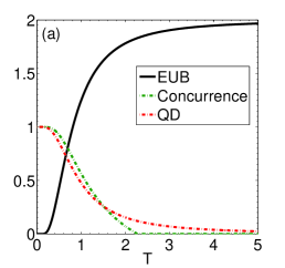
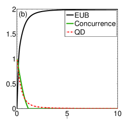
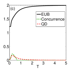
Figure 1: Entropic uncertainty bound, concurrence and quantum discord for an isolated quantum dot in terms of temperature with $B_{0}=1$, $\gamma=1$ (a)$k_{0}=10$. (b) $k_{0}=5$. (c) $k_{0}=3$.

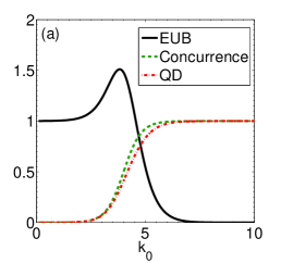
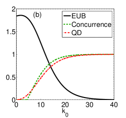
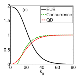
Figure 2: Entropic uncertainty bound, concurrence and quantum discord for an isolated quantum dot in terms of the deference between the energy of the singlet and triplet states $k_{0}$ with $B_{0}=1$, $\gamma=1$ (a)$T=0$. (b) $T=1$. (c) $T=2$.

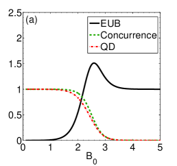
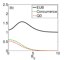
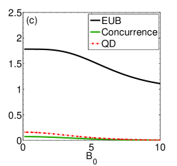
Figure 3: Entropic uncertainty bound, concurrence and quantum discord for an isolated quantum dot in terms of magnetic field $B_{0}$ with $k_{0}=10$, $\gamma=1$ (a)$T=0$. (b) $T=1$. (c) $T=2$.

Now, let us study the EUB, concurrence and quantum discord as a function of the temperature, the deference between the energy of the singlet and triplet states $k_{0}$, and Magnetic field $B_{0}$.

In Fig.1 we have plotted EUB and concurrence and QD versus temperature for specific value of $B_{0}$ and $k_{0}$. As can be seen EUB increases with increasing temperature, while quantum discord and concurrence decreases with increasing temperature. Of course, this is quite logical, because with the reduction of quantum correlation between parts $A$ and $B$, the value of uncertainty increases. It is also observed that the EUB increases with decreasing the parameter $k_{0}$. In Figs. 1(a) and 1(b) we have $\gamma B_{0}<k_{0}/4$, in this situation the ground state at zero temperature is $|\psi_{4}\rangle$, which is the maximally entangled state so for $k_{0}=10$ at zero temperature the system is maximally entangled. As the temperature increases, $|\psi_{4}\rangle$ will be mixed with the excited state, so the concurrence and QD monotically decreases from one to zero and uncertainty bound increases from zero to its maximum two. In Fig.1(c) we have $r>k_{0}/4$, the ground state of the quantum dot is $|\psi_{2}\rangle$, so the concurrence and QD is zero at zero temperature. This state will be mixed with excited state by increasing temperature. So, at first the concurrence and QD increases and then decreases.

In Fig.2, we have plotted EUB, concurrence and QD versus parameter $k_{0}$ for different value of temperature. As can be seen, the EUB start from non-zero value for $k=0$ and reaches to zero for large value of $k_{0}$. It is observed that at fixed temperature the concurrence and QD increases with increasing the parameter $k_{0}$. From Figs. 2(a) 2(b) and 2(c), it is observed that by increasing the temperature the EUB reaches to zero for larger value of $k_{0}$. It can also be seen that at fixed temperature when $k_{0}=0$ the state of the quantum dot is $|\psi_{2}\rangle$, so the concurrence and QD of quantum dot is zero. While for large value of $k_{0}$ at fixed temperature the state of the quantum dot is $|\psi_{4}\rangle$ and the concurrence and QD is equal to one.

In Fig.3, we have plotted EUB, concurrence and QD versus magnetic field $B_{0}$ for different value of temperature. In Fig.3(a), at zero temperature for $B_{0}=0$ the state of quantum dot is $|\psi_{4}\rangle$ while by increasing $B_{0}$ the state $|\psi_{4}\rangle$ will be mixed with the excited state, so the concurrence and QD monotically decreases from one to zero while EUB increases and reaches to fixed value. In Fig.3(b), at $T=1$ the state of quantum dot is partially mixed entangled state while for large value of $B_{0}$ at this temperature the state is $|\psi_{2}\rangle$ and the entanglement and QD is zero. From Fig. 3(b) it is also observed that the EUB reaches to fixed value for large amount of magnetic field. Finally from Figs. 1(a), 1(b) and 1(c), it is observed that the QD and concurrence decreases with increasing temperature while EUB increases with increasing the temperature.

6 conclusion

In this work we studied QMA-EUR and quantum correlations in a quantum dot system. We used concurrence and QD as practical criteria for quantum correlations. We studied the effect of temperature, the energy difference between the singlet and the triplet states, and the magnetic field on EUB, concurrence and QD. It was shown that the EUB can be reduced by decreasing the temperature. The situation for quantum coherence is quite different, it grows by reducing the temperature. It is observed that the EUB decreases with increasing the parameter $k_{0}$, while concurrence and QD increases with increasing this parameter. In studying the effects magnetic field $B_{0}$ on EUB it was observed that EUB grows by increasing the amount of magnetic field and after touch the summit, they become less to get a steady value for larger value of external magnetic. The concurrence and QD decreases with increasing magnetic field.

References

References

- [1] Werner R F 1989 Phys. Rev. A 40 4277
- [2] Hill S and Wootters W K 1997 Phys. Rev. Lett. 78 5022
- [3] Peres A 1996 Phys. Rev. Lett. 77 1413
- [4] Amico L, Fazio R, Osterloh A and Vedral V 2008 Rev. Mod. Phys. 80 517
- [5] Jaffali H and Holweck F 2019 Quantum Inf. Process. 18 133
- [6] Bennett C H, Brassard G, Crepeau C, Jozsa R, Peres A and Wooters W K 1993 Phys. Rev. Lett. 70 1895
- [7] Nielsen M A and Chuang I L 2000 Quantum Computation and Quantum Information (Cambridge: Cambridge University Press)
- [8] Bennett C H, Brassard G, Popescu S, Schumacher B, Smolin J A and Wootters W K 1996 Phys. Rev. Lett. 76 722
- [9] Pourkarimi M R and Rahnama M 2014 Int. J. Theor. Phys. 53 1415
- [10] Ekert A K 1991 Phys. Rev. Lett. 67 661
- [11] Bennett C H and Wiesner S J 1992 Phys. Rev. Lett. 69 2881
- [12] Sheng Y B, Pan J, Guo R, Zhou L and Wang L 2015 Sci. China Phys. Mech. Astron. 58 060301
- [13] Sheng Y B and Zhou L 2015 Sci. Rep. 5 7815
- [14] Zheng C and Wei S 2018 Int. J. Theor. Phys. 57 2203
- [15] Sheng Y B, Deng F G and Long G L 2010 Phys. Rev. A 82 032318
- [16] Sheng Y B and Zhou L 2013 Entropy 15 1776
- [17] Vidal G and Werner R F 2002 Phys. Rev. A 65 032314
- [18] Plenio M B 2005 Phys. Rev. Lett. 95 090503
- [19] Bennett C H, DiVincenzo D P, Smolin J A and Wootters W K 1996 Phys. Rev. A 54 3824
- [20] Bruss D 2002 J. Math. Phys. 43 4237
- [21] Christandl M and Winter A 2004 J. Math. Phys. 45 829
- [22] Vidal G and Tarrach R 1999 Phys. Rev. A 59 141
- [23] Coffman V, Kundu J and Wootters W K 2000 Phys. Rev. A 61 052306
- [24] Wong A and Christensen N 2001 Phys. Rev. A 63 044301
- [25] Vedral V, Plenio M B, Rippin M A and Knight P L 1997 Phys. Rev. Lett. 78 2275
- [26] Albeverio S and Fei S M 2001 J. Opt. B: Quantum Semiclass. Opt. 3 223
- [27] Carvalho A R R, Mintert F and Buchleitner A 2004 Phys. Rev. Lett. 93 230501
- [28] Mintert F, Kus M and Buchleitner A 2004 Phys. Rev. Lett. 92 167902
- [29] Akhound A, Haddadi S and Chaman Motlagh M A 2019 Mod. Phys. Lett. B 33 1950118
- [30] Barnum H and Linden N 2001 J. Phys. A: Math. Gen. 34 6787
- [31] Wei T C and Goldbart P M 2003 Phys. Rev. A 68 042307
- [32] Qun G Q, Chen X Y and Yun W Y 2014 Chin. Phys. B 23 050309
- [33] Love P J, Van den Brink A M, Smirnov A Y, Amin M H S, Grajcar M, Ilichev E, Izmalkov A and Zagoskin A M 2007 Quantum Inf. Process. 6 187
- [34] Montakhab A and Asadian A 2008 Phys. Rev. A 77 062322
- [35] Meyer D A and Wallach N R 2002 J. Math. Phys. 43 4273
- [36] Brennen G K 2003 Quantum Inf. Comput. 3 619
- [37] Scott A J 2004 Phys. Rev. A 69 052330
- [38] Haddadi S 2017 Int. J. Theor. Phys. 56 2811
- [39] Zhao C, Yang G and Li X 2016 Int. J. Theor. Phys. 55 1668
- [40] Ollivier H and Zurek W H 2001 Phys. Rev. Lett. 88 017901
- [41] Henderson L and Vedral V 2001 J. Phys. A 34 6899
- [42] Wang C Z, Li C X, Nie L Y and Li J F 2011 J. Phys. B: At. Mol. Opt. Phys. 44 015503
- [43] Chen Q, Zhang C, Yu S, Yi X X and Oh C H 2011 Phys. Rev. A 84 042313
- [44] Mazumdar S, Dutta S and Guha P 2019 Quantum Inf. Process. 18 169
- [45] Dakić B, Vedral V and Brukner C 2010 Phys. Rev. Lett. 105 190502
- [46] Cheng W W, Gong L Y, Shan C J, Sheng Y B and Zhao S M 2013 Eur. Phys. J. D 67 121
- [47] Qiang W C, Zhang H P and Zhang L 2016 Int. J. Theor. Phys. 55 1833
- [48] Hamdulla E, Abliz A, Aili M and Ma R 2018 Int. J. Theor. Phys. 57 965
- [49] Singh U and Pati A K 2014 Ann. Phys. 343 141
- [50] Li T, Ma T, Wang Y, Fei S M and Wang Z 2015 Int. J. Theor. Phys. 54 680
- [51] Jing N and Yu B 2017 Quantum Inf. Process. 16 99
- [52] Heisenberg W 1927 Z. Phys. 43 172
- [53] E. Schrodinger, Proc. Pruss. Acad. Sci. XIX, 296 (1930).
- [54] H. P. Robertson, Phys. Rev. 34, 163 (1929).
- [55] Kraus K 1987 Phys. Rev. D 35 3070
- [56] Maassen H and Uffink J B M 1988 Phys. Rev. Lett.
- [57] Berta M, Christandl M, Colbeck R, Renes J M and Renner R 2010 Nat. Phys. 6 659
- [58] Koashi M 2009 New J. Phys. 11 045018
- [59] Li X H, Zhao B K, Sheng Y B, Deng F G and Zhou H Y 2009 Int. J. Quantum Inf. 7 1479
- [60] Giovannetti V, Lloyd S and Maccone L 2011 Nat. Photon. 5 222
- [61] Pati A K, Wilde M M, Devi A R U, Rajagopal A K and Sudha S 2012 Phys. Rev. A 86 042105
- [62] Pramanik T, Chowdhury P and Majumdar A S 2013 Phys. Rev. Lett. 110 020402
- [63] Coles P J and Piani M 2014 Phys. Rev. A 89 022112
- [64] Liu S, Mu L-Z and Fan H 2015 Phys. Rev. A 91 042133
- [65] Zhang J, Zhang Y and Yu C-S 2015 Sci. Rep. 5 11701
- [66] Pramanik T, Mal S and Majumdar A S 2016 Quantum Inf. Process. 15 981
- [67] Adabi F, Salimi S and Haseli S 2016 Phys. Rev. A 93 062123
- [68] Adabi F, Salimi S and Haseli S 2016 Europhys. Lett. 115 60004
- [69] Huang J L, Gan W C, Xiao Y, Shu F W and Yung M H 2018 Eur. Phys. J. C 78 545
- [70] Dolatkhah H, Haseli S, Salimi S and Khorashad A S 2019 Quantum Inf. Process. 18 13
- [71] Haseli S, Dolatkhah H, Salimi S and Khorashad A S 2019 Laser Phys. Lett. 16 045207
- [72] Wang D, Huang A, Ming F, Sun W, Lu H, Liu C and Ye L 2017 Laser Phys. Lett. 14 065203
- [73] Wang D, Ming F, Huang A J, Sun W Y and Ye L 2017 Laser Phys. Lett. 14 095204
- [74] Wang D, Ming F, Huang A J, Sun W Y, Shi J D and Ye L 2017 Laser Phys. Lett. 14 055205
- [75] Huang A J, Shi J D, Wang D and Ye L 2017 Quantum Inf. Process. 16 46
- [76] Huang A J, Wang D, Wang J M, Shi J D, Sun W Y and Ye L 2017 Quantum Inf. Process. 16 204
- [77] Wang D, Huang A J, Hoehn R D, Ming F, Sun W Y, Shi J D, Ye L and Kais S 2017 Sci. Rep. 7 1066
- [78] Chen P F, Sun W Y, Ming F, Huang A J, Wang D and Ye L 2018 Laser Phys. Lett. 15 015206
- [79] Chen M N, Sun W Y, Huang A J, Ming F, Wang D and Ye L 2018 Laser Phys. Lett. 15 015207
- [80] Wang D, Shi W N, Hoehn R D, Ming F, Sun W Y, Kais S and Ye L 2018 Ann. Phys. (Berlin) 530 1800080
- [81] Ming F, Wang D, Huang A J, Sun W Y and Ye L 2018 Quantum Inf. Process. 17 9
- [82] Zhang Y, Fang M, Kang G and Zhou Q 2018 Quantum Inf. Process. 17 62
- [83] Ming F, Wang D, Shi W N, Huang A J, Sun W Y and Ye L 2018 Quantum Inf. Process. 17 89
- [84] Guo Y N, Fang M F and Zeng K 2018 Quantum Inf. Process. 17 187
- [85] Li J Q, Bai L and Liang J Q 2018 Quantum Inf. Process. 17 206
- [86] Ming F, Wang D, Shi W N, Huang A J, Du M M, Sun W Y and Ye L 2018 Quantum Inf. Process. 17 267
- [87] Zhang Y, Zhou Q, Fang M, Kang G and Li X 2018 Quantum Inf. Process. 17 326
- [88] Wang D, Shi W N, Hoehn R D, Ming F, Sun W Y, Ye L and Kais S 2018 Quantum Inf. Process. 17 335
- [89] Pourkarimi M R 2018 Int. J. Quantum Inf. 16 1850057
- [90] Pourkarimi M R 2019 Int. J. Quantum Inf. 17 1950008
- [91] Chen P F, Ye L and Wang D 2019 Eur. Phys. J. D 73 108
- [92] Shi W N, Ming F, Wang D and Ye L 2019 Quantum Inf. Process. 18 70
- [93] Yang Y Y, Sun W Y, Shi W N, Ming F, Wang D and Ye L 2019 Frontiers Phys. 14 31601
- [94] Chen M N, Wang D and Ye L 2019 Phys. Lett. A 383 977
- [95] Ming F, Wang D and Ye L 2019 Ann. Phys. 531 1900014
- [96] Koppens F H L, Buizert C, Tielrooij K J, Vink I T, Nowack K C, Meunier T, Kouwenhoven L P and Vandersypen L M K 2006 Nature 442 766
- [97] Nowack K C, Koppens F H L, Nazarov Y V and Vandersypen L M K 2007 Science 318 1430
- [98] Petta J R, Johnson A C, Taylor J M, Laird E A, Yacoby A, Lukin M D, Marcus C M, Hanson M P and Gossard A C 2005 Science 309 2180
- [99] Borras A and Blaauboer M 2011 Phys. Rev. B 84 033301
- [100] Hanson R and Awschalom D 2008 Nature 453 1043
- [101] Robledo L, Bernien H, van Weperen I and Hanson R 2010 Phys. Rev. Lett. 105 177403
- [102] Wootters W K 1998 Phys. Rev. Lett. 80 2245
- [103] I. L. Aleiner , P. W. Brouwer and L. I. Glazman, Phys. Rep. 358, 309 (2002).
- [104] L. Qin, , L. Tian and G. Yang, Int J Theor Phys 52, 4313–4322 (2013).
- [105] K. Berrada, Laser Phys. 23, 095201 (2013).
- [106] M. Pustilnik, , L. I. Glazman, Phys. Rev. B 64, 045328 (2001).