Multi-scale classification for electro-sensing††thanks: This work was supported by the SNF grant 200021-172483.
Abstract
This paper introduces premier and innovative (real-time) multi-scale method for target classification in electro-sensing. The intent is that of mimicking the behavior of the weakly electric fish, which is able to retrieve much more information about the target by approaching it. The method is based on a family of transform-invariant shape descriptors computed from generalized polarization tensors (GPTs) reconstructed at multiple scales. The evidence provided by the different descriptors at each scale is fused using Dempster-Shafer Theory. Numerical simulations show that the recognition algorithm we proposed performs undoubtedly well and yields a robust classification.
Keywords: Electro-sensing; weakly electric fish, classifier combination; shape classification; reconstruction.
1 Introduction
The biological behavior of weakly electric fish has been studied by scholars for years. These fish orient themselves at night in complete darkness by using electrosensory information, which makes these animals an ideal subject for developing bio-inspired imaging techniques. Such interest has motivated a huge number of studies addressing the active electro-sensing problem from many different perspectives since Lissmann and Machin’s work [1, 2, 3, 4, 5, 6, 7, 8]. One of the most noteworthy potential bio-inspired applications is in underwater robotics. Building autonomous robots with electro-sensing technology may supply unexplored navigation, imaging and classification capabilities, especially when the sight is unreliable due, for example, to the turbidity of the surrounding waters or the poor lighting conditions [9, 10].
From the mathematical point of view, the electro-sensing problem is to detect and locate the dielectric target and to identify its shape and material parameters given the current distribution over the skin of the fish. Ammari et al. [11] stated a rigorous mathematical model for treating the inverse problem of electro-sensing dielectric objects. They exploited the smallness of targets in order to apply the framework of asymptotic small-volume expansions. The electric current, which contains information on the target, is measured by a discrete number of receptors along the fish body. When enough measurements are collected, it is possible to recover the contracted generalized polarization tensors (CGPTs), which do encode information about the unknown target. One way in which the fish can acquire enough independent measurements is by exploiting the movement, i.e., by collecting several static measurements while swimming around the target [12]. In this way, it creates a synthetic-aperture view of the dielectric object that yields high-resolved reconstruction of its features. Although the inverse problem is severly ill-posed, classification works well. In [13] new shape descriptors, relying upon the CGPTs, which are invariants under rotations, translations, and scaling of the target, are found. In the previous works, a single circular trajectory around the target has been considered. In the two dimensional case, for small targets, the magnitude of the electric signal due to the presence of the target is of order , where is the length-scale, which is of the same order throughout the whole trajectory. In this type of setting it is natural to reconstruct the target’s features only up to some small order , which is called the resolving order. is essentially determined by the signal-to-noise ratio (SNR), that sets a limit to the fineness of the reconstruction we are capable of, see, for instance, [14]. It has been shown that the reconstruction is accurate enough to perform a dictionary matching approach for both homogeneous and inhomogeneous objects, see [15, 16].
The aim of this work is to improve the recognition capabilities of the fish by acquiring measurements at different length-scales on multiple circular orbits around the target. The main advantage of the multi-scale configuration is that the descriptors introduced in [14] can be compared at different orders up to the resolving order, which is increasing with respect to the length-scale. Therefore, selecting different comparison orders produces different classifiers. When many classifiers are available, the problem of combining them to enhance the classification capabilities naturally arises, see e.g. [17]. The approach we present in this paper relies on the so-called Transferable Belief Model (TBM), see, for instance, [18]. The output of a scoring-classifier, i.e., a list of numerical scores (a score for each element of the dictionary) that corresponds to the evidence at hand, can be converted into a belief assignment. Following [19, 20], a natural way to translate the scores into beliefs is to consider the Shannon’s entropy as a confidence factor associated to the evidence. Belief assignments are then combined by means of some combination rule, such as Dempster-Shafer rule, in order to obtain a synthetized new belief that pulls together all the information. This approach is particularly suitable for the electro-sensing problem hereabove. Since the fish is able to retrieve much more information about its shape and material parameters when approaching it, the classification is expected to be more robust as soon as multiple circular orbits are considered.
The paper is structured as follows. In Section 2, a preliminary description of the experimental design for electro-sensing is discussed. We show that the design matrix associated to the forward linear operator defined in [15] can be expressed as a generalized block Kronecker product by vectorization, see [21, 22]. A reflexive minimum norm g-inverse of the acquisition operator, arising in a natural way from the block Kronecker structure, is also used. This has been recently introduced in [22] in the context of bivariate polynomial regression. Based on Greville’s well known formulas in [23], this g-inverse provides a method to update recursively the estimates position after position right away.
In Section 3, a detailed analysis of the structure of the design matrix is carried out. In particular, the need of creating a synthetic-aperture view is readily understood by inspecting the rank of the design matrix. Assuming a circular acquisition setting, i.e., the fish collects the data swimming on a circular trajectory around the target, an estimate on the reconstruction error of the CGPTs is derived. The estimate has an upper bound depending on the length-scale, and it is formally equal to that given in [14]. Finally, issues related with limited-view data, i.e., data collected by receptors covering a limited angle of view, are discussed. In particular, a study of the spectrum of the matrix of receptors shows the impact of the angle of view on the reconstruction: the closer the angle of view is to , the more informative the estimate becomes. Furthermore, if the reconstruction order is small, the limited-view configuration has a minor impact on the reconstructed CGPTs.
In Section 4, the classification problem based on a multi-scale acquisition setting is addressed. In particular, measurements at different length-scales are used to improve the resolving power in the reconstruction of the CGPTs. As a matter of fact, the closer the orbit is to the target, the higher is the SNR, the higher is the order of CGPTs-based descriptors that can be used in the comparison. A matching algorithm, which generalizes the one proposed in [15] to the case study we consider, is presented. Firstly, a certain number of concentric orbits around the target are thoroughly chosen. On each orbit, a comparison between the theoretical and measured shape descriptors up to a properly chosen length-scale dependent order is required. Similarly to [15], the comparison is done by means of a given metric, and it yields a list of scores. The normalized list of scores produced on each orbit is converted into an evidence distribution, which is then stored. The Shannon’s entropy is used as a confidence factor, see [19, 20]. The evidence distributions computed along different orbits are subsequently combined by using the TBM conjunctive rule introduced in [24].
In Section 5 we perform numerical simulations in order to test the performance of the recognition algorithm, introduced in Section 4, on a particular dictionary of dielectric targets. The reported results show an enhancement of the recognition rate, corroborating the idea that combining descriptors at different length-scales makes the classification more robust. Both the minimum norm reflexive generalized inverse and the Moore-Penrose inverse are used in the reconstruction.
2 Model specification for electro-sensing
Let us now briefly summarise the model of electro-sensing derived in [11]: the body of the fish is , an open bounded set in , with smooth boundary , and with outward normal unit vector denoted by . The electric organ is a dipole inside or a sum of point sources inside satisfying the charge neutrality condition. The skin of the fish is very thin and highly resistive. Its effective thickness, that is, the skin thickness times the contrast between the water and the skin conductivities, is denoted by , and it is much smaller than the fish size. We assume that the conductivity of the background medium is one. We consider a smooth bounded target , and is a smooth bounded domain containing the origin. We assume that the conductivity of is , and define the contrast . In the presence of , the electric potential emitted by the fish is the solution to the following equations:
| (2.1) |
Here, is the characteristic function of , is the normal derivative, and denotes the limits from, respectively, outside and inside . Following [15], we introduce the function defined as
| (2.2) |
where on . and are the single- and double-layer potentials, respectively, defined in Appendix A. It is readily seen that the following representation formula holds:
| (2.3) |
where is the identity and is the Neumann-Poincaré operator associated to the target , see Appendix A.
2.1 Data acquisition system
In this section we aim at describing the data acquisition system, i.e., the experimental setting we shall adopt to solve the inverse problem.
As we briefly mentioned in the introduction, the fish use the movement in order to swim around the target, creating a synthetic aperture view.
Suppose that the scanning movement consists of a single circular orbit , with radius , the target being located at its center. On each orbit only a discrete number of positions accounts for the data acquisition process. Precisely, different positions are sampled along , and for each position the corresponding electric signal is measured by receptors on the skin, . Here and denote the solution to (2.1) and the function defined by (2.2), associated to the position , respectively.
This type of architecture resambles a multi-static SIMO (Single-Input Multi-Output) system.
| Symbol | Meaning |
|---|---|
| Fish body | |
| dipole moment | |
| electric organ | |
| -th receptor | |
| electric potential solution to (2.1) | |
| function defined in (2.2) | |
| number of receptors | |
| number of positions | |
| circular orbit |
For any orbit we get an matrix of data , which is called Multi-Static Response (MSR) matrix, whose -entry is defined as
| (2.4) |
Henceforth, we shall use the MATLAB colon notation for specifying sub-matrices of a given matrix. For instance, given matrix , we shall denote by [resp. ] the -th row [resp. the -th column] of .
2.2 Data acquisition operator
In order to simplify the notation, without loss of generality, we assume that the dielectric object is centered at the origin, and that the impedance of the fish is .
Theorem 2.1.
Consider different positions of the fish along the circular orbit of radius , with large enough, indexed by . Let be a set of receptors distributed on , the dipole located at with dipole moment , and . Then the following expansion holds:
| (2.5) |
where and are as in Definition A.5, ,
| (2.6) |
and
| (2.7) |
is the upper anti-diagonal block matrix of the CGPTs of order . Here, denotes the transpose of a matrix.
We define the length-scale associated to the orbit , i.e., the ratio between the size of the target and the distance .
A more careful analysis of the reminder in formula (2.5) shows that the remainder can be expressed in term of the length-scale , and written as . See Appendix C.
By Theorem 2.1, the rows of admit the following expansions:
| (2.8) |
where is the linear map defined by (2.5), i.e., , is the truncation order, and is the length-scale associated to the orbit . Thus, we can write the expansion of the complete MSR matrix as follows:
| (2.9) |
The linear map is the truncated output (or forward) operator.
The acquisition operator is defined by (2.5). More precisely, it can be written as
where
We define block matrices , by vertically stacking the matrices, as in Figure 1.
We are interested in estimating the matrix parameter from the MSR matrix . Therefore, we aim at solving the following minimization problem
| (2.10) |
where denotes the Frobenius norm of a matrix.
2.3 Generalized Kronecker form of the forward operator
In this section we vectorize the data acquisition operator in order to find a matrix representation.
Lemma 2.2.
Proof.
By definition,
Therefore
∎
Notice that the matrix defined by
| (2.11) |
is the unique matrix such that , for all .
Hence, minimization problem (2.10) assumes the following form
| (2.12) |
We aim at seeking a vector which is optimal in the least-squares sense.
As it is well known, the standard least-squares estimator for (2.12) is given by the Moore-Penrose inverse of , denoted by . If is full column rank, than
| (2.13) |
However, the special block Kronecker form of suggests to employ the following generalized inverse [22].
Theorem 2.3.
If and for , are full column rank, then
| (2.14) |
is a reflexive minimum norm g-inverse of . Here denotes the column-wise generalized Kronecker product defined in B.4, and † denotes the Moore–Penrose inverse.
Proof.
The proof is readily obtained by noticing that
∎
This particular generalized inverse is useful for solving (2.12) when lies in the range of [22]. Notice that is not the same as in general.
As we shall see later, the g-inverse given by (2.14) is particularly suitable for establishing a bound on the reconstruction error as well as for designing a recursive online estimation of the GPTs. Figure 2 schematically shows the computation of .
2.4 Online reconstruction
In this section we propose very simple formulas to efficiently perform an online reconstruction of the features.
By inspecting the form of the g-inverse given by (2.14) it is easy to see that, when a new position becomes available, the pseudoinverse of the augmented source matrix is the only term which needs to be recomputed. As shown in Figure 3, the pseudoinverses of the matrices corresponding to different positions intervene in without interfering with each other. Therefore we have the following result.
Lemma 2.4.
Let us denote the generalized inverse given by (2.14) for positions, and let be full column rank. Then
| (2.15) |
where
and
Proof.
Appending new positions affects only the factor , which can be updated by means of Greville’s recursive formula for the pseudoinverse, see [25]. ∎
3 Analysis of the design matrix
In this section we want to analyze in detail the form of the acquisition operator. As a result, we provide an in-depth study of the reconstruction.
Minimization problem (2.10) indicates that the null-space of the forward operator we studied so far is related to the capability of uniquely reconstructing the CGPTs, and, in the end, to the classification of a dielectric target.
3.1 Matrix of receptors
The matrix of receptors associated to the -th position is given by
In Appendix D.1, we show that is full column rank as soon as there are distinct receptors that are a general configuration in the sense of Remark D.1. Furthermore, we have the following Lemma [13].
Lemma 3.1.
distinct points distributed along a circular arc are a general configuration.
It is clear that a single position yields a design matrix which is not full column rank, no matter how many receptors are considered. However, collecting many electrostatic measurements at different positions ultimately enriches the column space of the matrix . As a matter of fact, if and for , are full column rank, proves to be a left-inverse and thus is full column rank as well.
3.2 Source vector
The row vector , which is referred to the source corresponding to the -th position, is defined by (2.5). For simplicity we consider the case , see (2.6).
Denote by
the unit vector orthogonal to the dipole moment , and be the location of the dipole.
We can naturally split into the pure dipole term and the distributed source term:
Here and are given as follows. Employing the product given in Definition B.3, define the block diagonal matrix
the diagonal matrix
and the row vector
Then
On the other hand, given points uniformly distributed on , we can discretize the integral defining and as follows
Consequently, defining the column vector
we get
Notice that reduces to if we choose the receptors as discretization points, i.e., .
In the end, the source vector can be written in the following form:
Let be the background solution, i.e., the potential in the absence of any target. When , the dipolar expansion derived in [11] yields
| (3.1) |
where . Such first order approximation of depends only on the geometry of the fish and on the position of the receptors.
3.3 Reconstruction error analysis
In this section we analyze the relative error in the reconstruction of the CGPTs when the g-inverse given by (2.14) is used, and the MSR data are acquired along a single circular orbit around the target.
Let be a random matrix with independent and identically distributed entries. Let be the matrix of the truncation errors. Recall that the entries of are of order , see (C.1).
The following multivariate multiple linear regression model for the measurements can be stated:
| (3.2) |
We restrict ourselves to the situation where the strength of the noise is enough to overpower the truncation error, which we disregard a posteriori for the rest of the analysis. More precisely, we assume that the strength of the noise satisfies
| (3.3) |
We define the signal to noise ratio (SNR) associated to the orbit as
Next, we vectorize equation (2.9). Define the vectorized error matrix
and response matrix, which is a multivariate normal vector given and for , namely,
Straightforward computations show that the covariance matrix of can be written as
| (3.4) |
Hereinafter, we assume that the receptors of are all distributed along one circular arc of radius . This assumption is justified by the fact that if we model the fish skin by two close circular arcs of radius and , with receptors on them, and we call its matrix of receptors, we can show that as .
Theorem 3.2.
For so that is non-zero, the relative error on the reconstructed CGPT satisfies
| (3.5) |
For vanishing , the error can be bounded by the right-hand side above with replaced by .
Proof.
We begin by observing that the absolute errors are the diagonal entries of Cov. In particular, the -th entry of the -th block matrix of Cov given by (3.4), i.e., , corresponds to CGPT . Define . By Lemma D.4 we have the inequality
On the other hand it is easy to show that
Therefore, we obtain the following estimate
The scaling property
together with the above control on show that the relative error satisfies (3.5).
∎
Remark 3.1.
In the proof we used the following inequality:
where the unspecified constant depends on the number of receptors and the angle of view . In the next section we analyze such dependency in the limit as , observing that the upper bound in (3.5) decays like .
Following [14], given the SNR and a tolerance level , the resolving order is defined as
It is readily seen that the resolving order satisfies
| (3.6) |
3.4 Angular resolution
In this section we want to discuss the issues related with the limited-view configuration, which is an intrinsic feature of the fish geometry. In order to get a grasp of how much the angle of view has an impact on the error estimate provided by Theorem 3.2, we restrict ourselves to a special configuration of receptors. In particular, we assume that there are receptors evenly distributed on an arc of the unit circle, with aperture angle , and we let go to .
Instead of studying the spectrum of we shall equivalently consider that of , where is defined in Appendix D.1, and denotes the matrix . For the sake of notation we refer to as the block matrix obtained from by permuting the columns as in Appendix D.1. We are interested in the asymptotic expansion of as . Hereinafter, we denote by .
With this particular geometry of receptors the limit matrix can be analytically computed:
where
and , .
Hence,
Applying the results contained in [26] we obtain the following result.
Lemma 3.3.
For large,
| (3.7) |
where the entries of depend only on the angle of view and the truncation order . Moreover, we have
| (3.8) |
where (resp. ) are the eigenvalues of the matrix (resp. ).
Remark 3.2.
Lemma 3.3 highlights the following facts. On one hand, as far as all the eigenvalues are away from zero, the reconstructed CGPTs have an upper bound on the relative error in (3.5) which decays like . More precisely, . On the other hand, when some eigenvalues occur to be very small (e.g. ), inequality (3.5) becomes uninformative, making us unable to predict the behavior of the relative error.
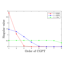
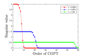
Figure 4 provides the distribution of , at different values of the reconstruction order and angles of view , as . Firstly, we clearly observe the asymptotic behavior of the spectrum stated by (3.8). Secondly, we notice that the effect of the limited-view configuration is reflected by the decaying of the eigenvalues of the matrix of receptors. As expected, the closer the angle of view is to , the more informative estimate (3.5) becomes. Furthermore, if is small, the angle of view has a minor impact on the reconstructed CGPTs.
 |
 |
| (a) | (b) |
4 Recognition
In the previous section, we established an upper bound on the reconstruction error which essentially depends on the length-scale of the acquisition orbit. As a consequence, the closer the fish gets to the target, the higher is the order of the features it can retrieve from the noisy measurements. This result suggests that, when it comes to classification, it is of preeminent importance to design recognition algorithms that exploit the information contained in measurements collected at multiple scales.
This section aims at presenting a novel multi-scale algorithm for target classification.
4.1 Complex CGPTs and shape descriptors
Let us briefly recall the definition of the shape descriptors.
We introduce convenient complex combinations of CGPTs. For any pair of indices , we introduce the following quantities
We define the complex CGPT matrices by
We call a dictionary a collection of standard shapes , centered at the origin, with characteristic size of order . We assume that a reference dictionary is initially given. Furthermore, suppose to consider a shape , which is unknown, that is obtained from an element by applying some unknown rotation , scaling and translation , i.e., .
Following [14], let . We define the following quantities
where the matrix is a lower triangular matrix with the -th entry given by
These quantities are translation invariant.
From , , for each pair of indices , we define the scaling invariant quantities:
The CGPT-based shape descriptors and are defined as:
where denotes the modulus of a complex number. Recall that and are invariant under translation, rotation, and scaling.
The details of this construction can be found in [14].
4.2 Multi-scale acquisition setting
Suppose that the scanning movement consists of concentric circular orbits , with radii respectively (ordered from the farthest to the nearest), the target being located at the common center. On each orbit only a discrete number of positions accounts for the data acquisition process, as described in Section 2.1. Precisely, different positions are sampled along the orbit , and for each position the corresponding electric signal is measured by receptors on the skin, .
Therefore, for any orbit we get the MSR matrix, whose -entry is defined as
| (4.1) |
Notice that so far the setting described above is very general, as no restriction has been given on the radii of the orbits yet.
Since the orbits are at different length-scales, it is clear that the closer the orbit is to the center, the stronger the MSR signal is. However, resorting to the error estimate on the reconstruction order (3.5), we are able to choose the orbits in such a way that the resolving order is enhanced.
In the multi-scale setting described above, formula (3.6) reads
| (4.2) |
where is the signal-to-noise ratio associated to the -th orbit.
Thus, a length-scale dependent resolving order is introduced, and obviously .
The noisy MSR matrix is given by the following formula
| (4.3) |
On each orbit , the CGPTs can be retrieved from the data (4.3), for instance, by either using the classical Moore-Penrose inverse or the generalized inverse given by (2.14). Moreover, we denote by the measured descriptors associated to the small target , which are computed from the reconstructed CGPTs .
Given a dictionary of standard shapes, which are denoted by , we want to design a matching algorithm, which generalizes the one proposed in [15] to a multi-scale configuration, see Figure 5. Firstly, a matching procedure as in [15] is required on each orbit, which consists of a comparison between the theoretical shape descriptors and the measured ones , up to a properly chosen length-scale dependent order .
Let us define the following scores:
| (4.4) |
where denotes the Frobenius norm of matrices, and .
For every , the scores (4.4) are used to perform the (local) comparison. Precisely, let be the vector formed by the elements of the dictionary, rearranged in ascending order according to , i.e.,
where is a permutation such that , for each .
Notice that, for efficiency reasons, it is convenient to cut the vector retaining the first components only, which are the elements of that produce the lowest scores.
Thus far we have just sorted the elements of the dictionary by matching the descriptors on each orbit separately. Instead of simply returning for each , that is in fact the algorithm in [14] applied on each orbit for a fixed reconstructing order , we aim at fusing the descriptors at the score level. Of course, the scores corresponding to descriptors which have different orders are not directly comparable. The proposed approach is inspired by [20].
We consider, for every orbit , the evidence distribution
where
Here, is a normalization constant such that the integral of the evidence distribution is , and is a smoothing parameter.
Besides , we may consider the Shannon’s entropy as a confidence factor. Tracing [19], we define
where is the Shannon entropy of the distribution .
Then, for each , we define the basic belief assignment (BBA)
quantifies the evidence given to each element of by the comparison of the descriptors on the -th orbit.
There exist many ways to fuse the evidence which are expressed as BBAs. One of the simplest formulas is the TBM conjunctive rule (E.4), which is associative. Therefore, we start with blending in with , obtaining . Then we combine with , obtaining
and so on, until we compute .
Finally, from the fused BBAs we define the pignistic probability (E.5), which is used to select the best candidate among the elements of .
5 Numerical results
In this section, we show some numerical results which illustrate how Algorithm 1 can significantly improve the robustness of the recognition procedure.
5.1 Setting
Let be a dictionary containing 8 standard shapes, as illustrated in Figure 7. Each solid shape is equipped with homogeneous conductivity having parameter (Circle, Ellipse, Triangle, Bent Ellipse, Curved Triangle, Gingerbread Man, Drop) whereas the dashed one (Ellipse) has conductivity . All the shapes have the same characteristic size, which is of order one.
The targets we are considering for the experiments are located at the origin as the standard shapes, and are obtained by scaling and rotating the elements of , with scaling coefficient and rotation angle chosen as and , respectively.
 |
 |
 |
 |
 |
 |
 |
 |
5.2 Experiment
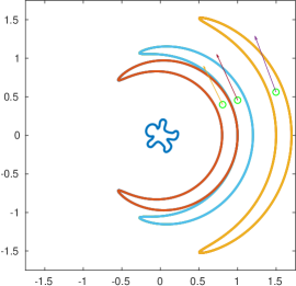
The data are acquired as described in Section 4.2. Precisely, given and three circular orbits around , of radii , , , respectively, we sample positions on each trajectory, and build the corresponding MSR matrices. We consider receptors evenly distributed on the the body of the fish.
In the numerical experiments the MSR data are simulated using the code developed in [27].
Remark 5.1.
In principle, the acquisition operator depends on the measurements, which is not a desirable property. In order to overcome this difficulty, we perform the numerical simulations using the surrogate acquisition operator obtained from the dipolar approximation (3.1).
The CGPTs are reconstructed on each orbit from the MSR matrix by exploiting either the g-inverse or the Moore-Penrose inverse . The reconstruction orders are set on , on , and on . The corresponding shape descriptors are then used as a rationale for building the BBAs and , with parameter , as described in Section 4.2. For efficiency reasons, positive mass is given only to the first best matching elements of .
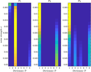
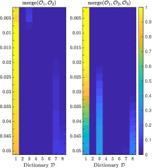
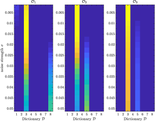
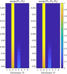
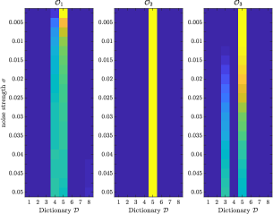
We study the robustness of the fused descriptors given by Algorithm 1 with moderate noise in the measurements. Precisely, given a target and , we test the recognition algorithm by considering experiments, and computing the frequencies.
The results arising from the beliefs produced on each orbit, i.e., and , are compared with the ones obtained from the fused beliefs synthetized by the TBM conjunctive rule, i.e., and .
5.2.1 Reconstruction by the generalized inverse
The results of this part are obtained by employing the reflexive minimum norm g-inverse of the acquisition operator given by (2.14) for the reconstruction of the CGPTs from the MSR data.
 |
 |
 |
 |
 |
 |
| 2 | 3 | 4 | 5 | 6 | 7 | 8 | ||
| 0.0021 | 0 | 0.8029 | 0 | 0 | 0 | 0 | 0.1950 | |
| 0.2805 | 0 | 0 | 0 | 0 | 0 | 0.7195 | 0 | |
| 0.0728 | 0 | 0.3582 | 0.0381 | 0.1400 | 0 | 0.0088 | 0.3821 | |
| 0.8288 | 0 | 0 | 0 | 0 | 0 | 0.0834 | 0.0878 | |
| 0.3575 | 0 | 0.3585 | 0.0001 | 0.0013 | 0 | 0.0174 | 0.2652 |
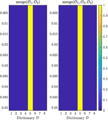
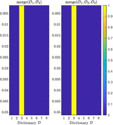
Looking at Table 2 we can clearly see that the combination of classifiers outperforms each classifier. In particular we can see that combining the classifiers on and yields a great improvement in the recognition already.
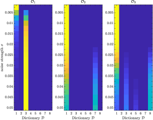
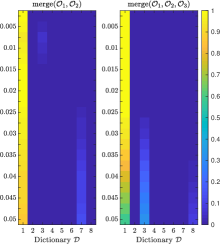
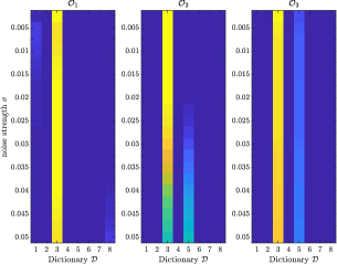
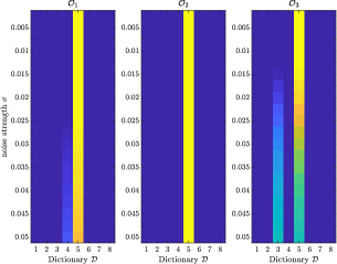
Tables 3 and 4 refer to the Triangle (3) and the Curved Triangle (5). Because of their similar silhouette, they are troublesome from a dictionary approach point of view [16], and thus it is interesting to have a close look at what happens in both cases.
| 1 | 2 | 4 | 5 | 6 | 7 | 8 | ||
| 0.0006 | 0 | 0.4229 | 0 | 0.0115 | 0 | 0 | 0.5650 | |
| 0 | 0 | 0.3371 | 0 | 0.6629 | 0 | 0 | 0 | |
| 0 | 0 | 0.8038 | 0 | 0.1962 | 0 | 0 | 0 | |
| 0 | 0 | 0.7519 | 0 | 0.2382 | 0 | 0 | 0.0099 | |
| 0 | 0 | 0.7702 | 0 | 0.2297 | 0 | 0 | 0.0001 |
| 1 | 2 | 3 | 4 | 6 | 7 | 8 | ||
|---|---|---|---|---|---|---|---|---|
| 0 | 0 | 0 | 0.5015 | 0.4650 | 0 | 0.0002 | 0.0333 | |
| 0 | 0 | 0.0064 | 0 | 0.9936 | 0 | 0 | 0 | |
| 0 | 0 | 0.5395 | 0 | 0.4605 | 0 | 0 | 0 | |
| 0 | 0 | 0.0011 | 0.0016 | 0.9967 | 0 | 0 | 0.0006 | |
| 0 | 0 | 0.0017 | 0 | 0.9983 | 0 | 0 | 0 |
It is worth noticing that in Table 3 the highest frequency is not attained by the fusion of the descriptors. Instead, the third orbit alone produces the best matching. However, merging all the three BBAs enhances considerably the classification success rate in the worst case scenario, which is strikingly lower than the rate in the best case scenario.
Clearly, this is not a drawback of our method. As a matter of fact, since in advance we don’t know which classifier performs the best, the above results indicate that using their combination is a valid -as well as natural- trade-off.
5.2.2 Reconstruction by the Moore-Penrose inverse
In this part we make use of the Moore-Penrose inverse to reconstruct the CGPTs from the MSR simulated data, as shown in (2.13).
 |
 |
 |
 |
 |
 |
| 2 | 3 | 4 | 5 | 6 | 7 | 8 | ||
| 0.0106 | 0 | 0.9885 | 0 | 0 | 0 | 0 | 0.0009 | |
| 0.4889 | 0 | 0 | 0 | 0 | 0 | 0.5111 | 0 | |
| 0.1784 | 0 | 0.2565 | 0.0138 | 0.0817 | 0 | 0.0021 | 0.4675 | |
| 0.8729 | 0 | 0 | 0 | 0 | 0 | 0.1270 | 0.0001 | |
| 0.5914 | 0 | 0.3185 | 0.0001 | 0.0016 | 0 | 0.0067 | 0.0817 |
| 1 | 2 | 4 | 5 | 6 | 7 | 8 | ||
|---|---|---|---|---|---|---|---|---|
| 0.0033 | 0 | 0.9121 | 0 | 0 | 0 | 0 | 0.0846 | |
| 0 | 0 | 0.5027 | 0 | 0.4973 | 0 | 0 | 0 | |
| 0 | 0 | 0.7652 | 0 | 0.2346 | 0 | 0.0002 | 0 | |
| 0 | 0 | 0.9933 | 0 | 0.0046 | 0 | 0 | 0.0021 | |
| 0 | 0 | 0.9910 | 0 | 0.0090 | 0 | 0 | 0 |
| 1 | 2 | 3 | 4 | 6 | 7 | 8 | ||
|---|---|---|---|---|---|---|---|---|
| 0 | 0 | 0 | 0.1476 | 0.8512 | 0 | 0 | 0.0012 | |
| 0 | 0 | 0.0013 | 0 | 0.9987 | 0 | 0 | 0 | |
| 0 | 0 | 0.4855 | 0 | 0.5145 | 0 | 0 | 0 | |
| 0 | 0 | 0 | 0.0008 | 0.9992 | 0 | 0 | 0 | |
| 0 | 0 | 0.0001 | 0 | 0.9999 | 0 | 0 | 0 |
While the g-inverse lacks of the property of being a least-square g-inverse, the Moore-Penrose provides the solution to the minimization problem (2.12). Therefore, it is not surprising that the classification rates obtained by using the latter are generally better than the ones resulting from using .
6 Concluding remarks
In this paper, we have presented a dictionary-matching approach for classification in electro-sensing that takes advantage of measurements at different length-scales. We have performed a careful analysis of the acquisition operator that was not available yet. In particular, by exploiting its peculiar block Kronecker form, we have studied its rank and established a length-scale dependent estimate on the reconstruction error. We have also discussed to which extent the limited-view configuration impacts on predicting the committed error.
Acknowledgments
The authors gratefully acknowledge Prof. H. Ammari for his guidance. During the preparation of this work, the authors were financially supported by a Swiss National Science Foundation grant (number 200021-172483).
Appendix A Generalized polarization tensors and boundary layer potentials
We briefly summarise some fundamental concepts that are essential for understanding the problem. For further references see [11, 13, 15, 16].
Let be a simply-connected bounded domain. We assume .
Definition A.1.
Denote by the fundamental solution of the Laplacian in , i.e.,
Definition A.2.
For any , the single- and double-layer potentials on are given by the following formulas:
Recall that for , the functions and are harmonic functions in .
Definition A.3.
The operator and its -adjoint are given by the following formulas:
where p.v. stands for the Cauchy principal value.
is also known as the Neumann-Poincaré operator.
We introduce the generalized polarization tensor (GPT).
Definition A.4.
Let be multi-indices. We define the generalized polarization tensor associated with the domain and the contrast by
where is the identity operator.
We can also define the contracted generalized polarization tensor (CGPT) as follows.
Definition A.5.
Let . We define the contracted generalized polarization tensors by
where the real numbers and are defined by the following relation
Appendix B Kronecker products and generalized inverses
Let us denote by the space of matrices.
Definition B.1 (vec operator).
Given a matrix , define the vectorization operator as follows
| (B.1) |
Definition B.2 (Kronecker product).
Given and , define
| (B.2) |
For all matrices , and such that the product is well defined we have
| (B.3) |
We introduce a generalized Kronecker product.
Definition B.3 (Generalized Kronecker product [28, 22]).
Given a matrix () and a set of matrices () we define the matrix ( ) as
| (B.4) |
Notice that in [28] the factors are swapped compared to this definition. The reason is that, unlike us, they considered a left Kronecker product.
Definition B.4 (Generalized column-wise Kronecker product).
Given a matrix () and a set of matrices () we define the matrix ( ) as
| (B.5) |
Definition B.5 (Moore-Penrose inverse).
The Moore-Penrose inverse of the matrix () is the unique matrix () satisfying the four Penrose conditions:
-
1.
,
-
2.
,
-
3.
,
-
4.
.
A matrix satisfying (1) is called a generalized inverse or g-inverse.
A matrix satisfying (1) and (2) is called reflexive g-inverse.
A matrix satisfying (1) and (3) is called least-square g-inverse.
A matrix satisfying (1) and (4) is called minimum norm g-inverse.
Appendix C Reminder in the asymptotic expansion (2.5)
Let be the length-scale. By definition, the truncation error at the receptor is given by
The asymptotic behavior of in the far-field regime is assessed by the following proposition.
Proposition C.1.
For we have the following asymptotic behavior
| (C.1) |
Proof.
Hereinafter, we simplify our notation by fixing the index position , i.e., , , .
Let us define . The truncation error can be expressed as
| (C.2) |
We want to estimate each term separately.
Denote the first term:
| (C.3) |
We have
Now we estimate the term
| (C.4) |
Recall the integral form of the reminder of Taylor’s formula:
then
It is immediate to show that
Assume , . By using formulas for the derivatives of we get
| (C.5) |
hence
Therefore
∎
Appendix D Technical estimates
D.1 Uniqueness results
In this section, we show that the matrix of receptors is full column rank. We begin by observing that is closely related to a special Vandermonde matrix of the form
| (D.1) |
Matrices of this type are of interest when dealing with univariate polynomial interpolation on complex conjugate points. We introduce the map
is known in the literature as Kelvin transform. Then the entries of (D.1) are defined as follows: for any receptor we set .
To relate with we introduce other two matrices. By employing the product defined in Definition B.3, consider the diagonal scaling matrix
and, by setting , define the complex block diagonal matrix:
It can be easily verified that .
Observe that there exists a permutation matrix such that .
Lemma D.1.
Let be the square sub-matrix of obtained by considering the first rows. Then
where . Since and , it is clear that
where .
The set is an hyper-surface in the affine space .
Definition D.1.
A finite set of points , , is called general configuration if the point doesn’t lie on .
Proposition D.2.
Suppose there are receptors such that are a general configuration. Then is of maximal rank.
Proof.
Without loss of generality, let are a general configuration. From Lemma D.1 it follows that is a real multivariate polynomial and it doesn’t vanish when evaluated at the points . ∎
Remark D.1.
By an abuse of definition, a set of points such that is a general configuration, shall be called a general configuration likewise.
D.2 Moore-Penrose inverse of
For , let be the following rotation matrix:
If we assume that the body of the fish lies in a thin annulus around the orbit of radius while swimming around the target, then the form of the design matrix can be simplified. In this case, if (3.1) is used, the information on the fish concerning its geometry and its electric field can be separated from the “kinematics”. Easy calculations show that
where
Moreover, given angle of , we have
Hereinafter, we assume that the fish moves with its electric organ along on a circular orbit of radius .
Recall that
By using the rotational symmetry of the configuration and the notation hereabove, we rewrite and as follows:
and
Here, is given as in Section 3.2 by
Finally,
and
Hereinafter, we assume that is non-zero for each . In the far field regime this assumption guarantees that the GPTs can be retrieved up to order . It will become clear soon that this condition also makes full column rank, allowing to compute its Moore-Penrose inverse as
We have the following lemma.
Lemma D.3.
For and , we have
| (D.2) |
Proof.
Let us denote the row vector by . We need to compute , that is
Since , the product boils down to
Notice that the receptor is . Since , for some small, we assume that . As a consequence, we can factorize as
where is a Vandermonde-type matrix with nodes on the unit disk .
We obtain
It is immediate to see that
where
Let us denote by .
To prove estimate (D.2), we rely on the following inequality:
| (D.3) |
By a straightforward calculation, it is immediate to see that
| (D.4) |
and
| (D.5) |
Finally, we investigate the Frobenius norm of . For , we observe that
where
For , we have
Therefore, can be written as follows:
where
Notice that requiring to be invertible is equivalent to saying that each , and thus each , is non-zero. For this reason, the initial assumption on implies that is invertible (see [15]) and thus, for large enough, is full column rank. Since , we have [29]
Since is unitary, . Hence
| (D.6) |
Finally, inequality (D.3) together with estimates (D.4), (D.5) and (D.6) shows that satisfies (D.2). ∎
We are now ready to estimate the dependency of on and . For large enough, we observe that the leading order term of is .
Lemma D.4.
For , we have
Proof.
Let us denote the matrix by . Observe that both and are independent of . We have
∎
Appendix E Transferable Belief Model
In this appendix we present some basic definitions from evidence theory. In particular, we shall consider the Transferable Belief Model (TBM), see [30]. This theory doesn’t require any underlying probability space.
In the context of dictionary classification, the frame of discernment is usually modeled as a finite set , which is called dictionary.
A belief function is a function such that:
-
1.
;
-
2.
for all ,
(E.1) -
3.
.
A basic belief assignment (BBA) is a function such that
The value for is called the basic belief mass (bbm) given to . This is a part of the agent’s belief that supports , and that, due to lack of information, does not support any strict subset of . If then is called focal set. Observe that it is allowed to allocate positive BBM to , i.e., .
The basic belief assignment (BBA) related to a belief function is the function such that:
| (E.2) |
Moreover, there is a one-to-one correspondence between and via the following formula
| (E.3) |
that is, is obtained by summing all BBMs given to subsets with , and it quantifies the total amount of justified specific support given to .
Let and be two BBAs, we define the TBM conjunctive combination of the two as
| (E.4) |
In the TBM model, from a decision-making point of view we need to resort to a probability distribution in order to select the most reliable hypothesis in . Such function is called pignistic probability, and is defined as
| (E.5) |
The term pignistic stresses the fact that the only purpose of these probabilities is that of forcing a decision.
References
- [1] C. Assad, Electric field maps and boundary element simulations of electrolocation in weakly electric fish. PhD thesis, 1997.
- [2] D. Babineau, A. Longtin, and J. Lewis, “Modeling the electric field of weakly electric fish,” The Journal of experimental biology, vol. 209, pp. 3636–51, 10 2006.
- [3] R. Budelli and A. Caputi, “The electric image in weakly electric fish: perception of objects of complex impedance,” Journal of Experimental Biology, vol. 203, no. 3, pp. 481–492, 2000.
- [4] C. Ling, L. H. Jonathan, K. Rüdiger, and E. N. Mark, “Modeling signal and background components of electrosensory scenes,” Journal of Comparative Physiology A, vol. 191, pp. 331–345, 2005.
- [5] M. Maciver, The computational neuroethology of weakly electric fish: Body modeling, motion analysis, and sensory signal estimation. PhD thesis, 2001.
- [6] M. MacIver, N. Sharabash, and M. Nelson, “Prey-capture behavior in gymnotid electric fish: Motion analysis and effects of water conductivity,” Mar. 2001.
- [7] B. Rasnow, C. Assad, M. E. Nelson, and J. M. Bower, “Simulation and measurement of the electric fields generated by weakly electric fish,” in Advances in Neural Information Processing Systems 1 (D. S. Touretzky, ed.), pp. 436–443, Morgan-Kaufmann, 1989.
- [8] G. von der Emde, S. Schwarz, L. Gomez, R. Budelli, and K. Grant, “Electric fish measure distance in the dark,” Nature, vol. 395, pp. 890–894, 1998.
- [9] G. von der Emde, “Active electrolocation of objects in weakly electric fish,” Journal of Experimental Biology, vol. 202, no. 10, pp. 1205–1215, 1999.
- [10] O. Curet, N. Patankar, G. Lauder, and M. Maciver, “Aquatic manoeuvering with counter-propagating waves: A novel locomotive strategy,” J. R. Soc. Interface, vol. 8, pp. 1041–1050, 2011.
- [11] H. Ammari, T. Boulier, and J. Garnier, “Modeling active electrolocation in weakly electric fish,” SIAM Journal on Imaging Sciences, vol. 6, no. 1, pp. 285–321, 2013.
- [12] H. Ammari, T. Boulier, J. Garnier, and H. Wang, “Mathematical modelling of the electric sense of fish: the role of multi-frequency measurements and movement,” Bioinspiration & Biomimetics, vol. 12, p. 025002, jan 2017.
- [13] H. Ammari, J. Garnier, W. Jing, H. Kang, M. Lim, K. Sølna, and H. Wang, Mathematical and Statistical Methods for Multistatic Imaging. Cham: Springer International Publishing, 2013.
- [14] H. Ammari, T. Boulier, J. Garnier, W. Jing, H. Kang, and H. Wang, “Target identification using dictionary matching of generalized polarization tensors,” Foundations of Computational Mathematics, vol. 14, pp. 27–62, Feb 2014.
- [15] H. Ammari, T. Boulier, J. Garnier, and H. Wang, “Shape recognition and classification in electro-sensing,” Proceedings of the National Academy of Sciences, vol. 111, no. 32, pp. 11652–11657, 2014.
- [16] A. Scapin, “Electro-sensing of inhomogeneous targets,” Journal of Mathematical Analysis and Applications, vol. 472, no. 2, pp. 1872 – 1901, 2019.
- [17] L. Xu, A. Krzyzak, and C. Y. Suen, “Methods of combining multiple classifiers and their applications to handwriting recognition,” IEEE Transactions on Systems, Man, and Cybernetics, vol. 22, pp. 418–435, May 1992.
- [18] D. Mercier, G. Cron, T. Denoeux, and M. Masson, “Fusion of multi-level decision systems using the transferable belief model,” in 2005 7th International Conference on Information Fusion, vol. 2, pp. 8 pp.–, July 2005.
- [19] V.-N. Huynh, N. T. Tri, and C. A. Le, “Adaptively entropy-based weighting classifiers in combination using dempster-shafer theory for word sense disambiguation,” Comput. Speech Lang., vol. 24, pp. 461–473, 2010.
- [20] V. Mondéjar-Guerra, R. Muñoz-Salinas, M. Marín-Jiménez, A. Carmona-Poyato, and R. Medina-Carnicer, “Keypoint descriptor fusion with dempster–shafer theory,” International Journal of Approximate Reasoning, vol. 60, pp. 57 – 70, 2015.
- [21] P. A. Regalia and M. K. Sanjit, “Kronecker products, unitary matrices and signal processing applications,” SIAM review, vol. 31, no. 4, pp. 586–613, 1989.
- [22] A. Marco, J.-J. Martínez, and R. Viaña, “Least squares problems involving generalized kronecker products and application to bivariate polynomial regression,” Numerical Algorithms, Sep 2018.
- [23] T. Greville, “Some applications of the pseudoinverse of a matrix,” SIAM Review, vol. 2, no. 1, pp. 15–22, 1960.
- [24] P. Smets and R. Kennes, The Transferable Belief Model, pp. 693–736. Berlin, Heidelberg: Springer Berlin Heidelberg, 2008.
- [25] J. Zhou, Y. Zhu, X. R. Li, and Z. You, “Variants of the greville formula with applications to exact recursive least squares,” SIAM Journal on Matrix Analysis and Applications, vol. 24, no. 1, pp. 150–164, 2002.
- [26] A. Deif, “The generalized inverse of a perturbed singular matrix,” Zeitschrift Fur Angewandte Mathematik Und Physik - ZAMP, vol. 34, pp. 291–300, 05 1983.
- [27] H. Wang, “Shape identification in electro-sensing.” https://github.com/yanncalec/SIES, 2013.
- [28] P. Regalia and M. Sanjit, “Kronecker products, unitary matrices and signal processing applications,” SIAM Review, vol. 31, no. 4, pp. 586–613, 1989.
- [29] A. Ben-Israel, “On error bounds for generalized inverses,” SIAM Journal on Numerical Analysis, vol. 3, 12 1966.
- [30] P. Smets, “The nature of the unnormalized beliefs encountered in the transferable belief model,” in Uncertainty in Artificial Intelligence (D. Dubois, M. P. Wellman, B. D’Ambrosio, and P. Smets, eds.), pp. 292 – 297, Morgan Kaufmann, 1992.