SuppReferences
Scale interactions and anisotropy in Rayleigh-Taylor turbulence
Abstract
We study energy scale-transfer in Rayleigh-Taylor (RT) flows by coarse-graining in physical space without Fourier transforms, allowing scale analysis along vertical direction. Two processes are responsible for kinetic energy flux across scales: baropycnal work , due to large-scale pressure gradients acting on small-scales of density and velocity, and deformation work , due to multi-scale velocity. Our coarse-graining analysis shows how these fluxes exhibit self-similar evolution that is quadratic-in-time, similar to RT mixing layer. We find that is a conduit for potential energy, transferring energy non-locally from the largest scales to smaller scales in the inertial range where takes over. In 3D, continues a persistent cascade to smaller scales, whereas in 2D re-channels the energy back to larger scales despite the lack of vorticity conservation in 2D variable density flows. This gives rise to a positive feedback loop in 2D-RT (absent in 3D) in which mixing layer growth and the associated potential energy release are enhanced relative to 3D, explaining the oft-observed larger values in 2D simulations. Despite higher bulk kinetic energy levels in 2D, small inertial scales are weaker than in 3D. Moreover, the net upscale cascade in 2D tends to isotropize the large-scale flow, in stark contrast to 3D. Our findings indicate the absence of net upscale energy transfer in 3D-RT as is often claimed; growth of large-scale bubbles and spikes is not due to “mergers” but solely due to baropycnal work .
1 Introduction
The Rayleigh-Taylor (RT) instability occurs when a heavy fluid is on top of a light fluid in the presence of gravity, or more generally when a light fluid is accelerated against a heavy fluid (Rayleigh, 1883; Taylor, 1950). It is of both fundamental interest and practical importance in many fields and applications. For example, RT instability plays a leading role in the propagation of the thermonuclear flame front in supernova explosions (Hillebrandt & Niemeyer, 2000), and is a main obstacle towards achieving ignition in inertial confinement fusion (ICF) (Betti & Hurricane, 2016).
Any reasonable person would probably agree that modeling such RT unstable 3D systems using 2D simulations is inferior to using 3D simulations. Yet, what aspects of the dynamics may be misrepresented in a 2D simulation? How might such misrepresentation affect the overall modeled system and conclusions? Answers to these questions are not readily clear, which perhaps explains why 2D-RT modeling still being relied upon due to its lower computational costs. This holds to varying degrees in the fluids literature (e.g. Wei et al., 2017; Zhang et al., 2018c; Bestehorn, 2020), the astrophysics literature (e.g. Kotake et al., 2018; Just et al., 2018; Chen et al., 2020), among several others. For example, in plasma physics research, 2D simulations are still the main “work horse” for experimental design in inertial fusion to this day (e.g. Hopkins et al., 2018; Weber et al., 2020; Anderson et al., 2020; Meaney et al., 2020; Carpenter et al., 2020). ICF modelers aim to predict or postdict results from shots (i.e. experiments) in the laboratory. Given finite computational resources, the choice is often to include more physical processes in simulations at the expense of conducting them in 2D, despite the recognition that 3D modeling is preferable. Such decisions are often made in large part because the trade-offs between 2D and 3D flow physics are not as clear as the trade-offs between whether or not to include laser deposition physics, hohlraum physics, or resolve effects such as from the “tent” or “stalk-mount” (Clark et al., 2016). A main aim of this work is to highlight the stark differences between 2D- and 3D-RT flow physics.
Based on constant-density incompressible homogeneous 2D turbulence (Kraichnan, 1967), it is sometimes argued that due to vorticity (or enstrophy) conservation, we should expect a net upscale cascade in 2D-RT (e.g. Cabot, 2006). However, RT flows do not conserve vorticity, even in 2D, due to baroclinicity. Therefore, extending such an argument (Kraichnan, 1967) from constant-density homogeneous flows to inhomogeneous flows with variable density remains dubious. Why should we expect 2D-RT flows to yield an upscale cascade if the underlying cause for such a phenomenon, namely vorticity conservation, does not hold in variable density flows? One contribution of this work is to demonstrate, via a direct measurement of the cascade, that a net upscale cascade does indeed exist in 2D-RT flows with significant density variation, despite the lack of vorticity conservation. Moreover, we show that such an upscale cascade leads to a spurious positive feedback loop that is absent from 3D-RT.
Even in 3D-RT, there is considerable confusion on whether kinetic energy is transferred upscale or downscale. In many studies discussing RT flows in 3D, there is a pervasive notion that the generation of successively larger bubbles following the presence of smaller ones is due to an upscale cascade of energy which causes small bubbles to “merge” into larger ones. This seems to pervade several research areas, such as studies motivated by ICF (e.g. Shvarts et al. (1995); Alon et al. (1995); Ofer et al. (1996); Oron et al. (2001); Zhou et al. (2003)), or magnetic fusion (e.g. Douglas et al., 1998), or astrophysics (e.g. Joggerst et al. (2010); Porth et al. (2014)), or fundamental fluid dynamics (e.g. Abarzhi (1998); Cheng et al. (2002); Cabot (2006)). According to such a narrative, the small-scales are the source of energy feeding and sustaining the large-scales, even in 3D. A main result of our paper is measuring the net energy transfer in 3D-RT directly and showing that it is downscale rather than upscale. We show that the emergence of successively larger scales in 3D-RT is driven not by an upscale cascade but by baropycnal work.
1.1 Brief Overview of RT Flows
RT instability driven flows occur when a heavy fluid is accelerated against a light fluid and is manifested by the formation of upward rising bubbles of the light fluid and downward sinking spikes of the heavy fluid. There are several valuable reviews on the topic (Sharp, 1984; Kull, 1991; Abarzhi, 2010; Zhou, 2017a, b; Boffetta & Mazzino, 2017; Livescu, 2020).
RT flows are usually categorized either as single-mode, in which the initial perturbation consists of a single sinusoidal wave spanning the domain, or as multi-mode, in which the initial perturbation has a broad spectrum. During the early linear stage of evolution, single-mode RT grows exponentially before nonlinear effects set in and its growth rate plateaus (Layzer, 1955; Goncharov, 2002), then undergoes further acceleration (Wei & Livescu, 2012) due to vorticity production (Ramaprabhu et al., 2012; Bian et al., 2020). In contrast, multi-mode RT is expected to evolve as a set of uncoupled modes during the linear stage before mode-coupling sets in due to nonlinear interactions between different scales (Dimonte, 2004). Multi-mode RT becomes turbulent with a wide range of scales, characterized by a quadratic-in-time self-similar growth of the mixing layer between the heavy and light fluids (e.g. Ristorcelli & Clark, 2004).
The self-similar stage is dominated by growth of the largest structures present at any given time. The self-similar dynamics has been divided into two categories, depending on the initial perturbation spectrum (Glimm & Li, 1988; Shvarts et al., 1995; Dimonte, 2004; Dimonte et al., 2005): (i) when long-wavelength modes grow directly from perturbations present at the initial time. This category is sometimes called “bubble competition,” and is believed to be sensitive to initial conditions (Dimonte et al., 2004; Zhou, 2017a). (ii) when long-wavelength modes are absent at the initial time and grow from the interaction of short-wavelength perturbations present initially. This self-similar category is often called “bubble merger,” and is believed to be insensitive to initial conditions (e.g. Ramaprabhu et al., 2005). In both categories, growth of the RT mixing layer between the heavy and light fluids is quadratic-in-time of the mixing layer, but differing in the growth proportionality constant, . Whether describing single-mode or multi-mode RT, the primary focus of past studies has been the RT growth rates at different times (e.g. Dimonte et al., 2004), which is of foremost importance in applications such as fusion. Our focus here is rather different and aimed at understanding the energy pathways across scales.
1.2 Energy Scale-Transfer in Boussinesq RT Turbulence
RT turbulent flows are unsteady, inhomogeneous, and anisotropic, and it is unclear that the traditional cascade picture from Kolmogorov’s theory holds (Alexakis & Biferale, 2018; Zhou, 2021). A motivation of this paper is to measure the cascade in RT flows directly, without having to rely on traditional tools from turbulence theory, such as Fourier analysis or structure functions, which rest on assumptions that do not hold in RT turbulence.
Several previous works (Zhou, 2001; Chertkov, 2003; Ristorcelli & Clark, 2004; Boffetta et al., 2009; Zhou et al., 2016; Livescu et al., 2010) have made valuable contributions to addressing this problem, the majority of which focused on low Atwood number incompressible RT flows described by the Boussinesq model. In this model, density variation is negligible except in the buoyancy term of the momentum equation, and the associated velocity field is solenoidal.
An important phenomenological theory on Boussinesq RT turbulence was proposed by Chertkov (2003), but had to assume a (quasistationary) constant kinetic energy flux to small scales and a balance between buoyancy and the time derivative of velocity. Subsequently, Boffetta et al. (2009) carried out 3D Boussinesq RT simulations and analyzed the energy budget equations in Fourier space, where a Fourier transform was applied in the homogeneous (horizontal) directions. Simulations of 2D Boussinesq RT flows were also analyzed using both Fourier analysis (Boffetta et al., 2012) and a filtering approach in physical space (Zhou et al., 2016) similar to what we do here for the more general (non-Boussinesq) problem. Boffetta et al. (2012) and Zhou et al. (2016) both concluded that there is an inverse energy cascade and a forward enstrophy cascade in 2D Boussinesq RT flows.
Moreover, Boffetta et al. (2012) studied the 3D to 2D transition in high aspect ratio RT simulations, with a domain size , and inferred the presence of a transition scale. Using Fourier analysis in the homogeneous directions, Boffetta et al. (2012) concluded that the flow has 2D-like evolution at (horizontal) scales larger than the transition scale and seems to follow a Bolgiano-Obukhov phenomenology, characterized by an inverse energy cascade, while smaller scales evolve as in 3D following the Kolmogorov-Obukhov phenomenology, characterized by a forward energy cascade.
These studies have established a self-consistent picture of phenomenological Boussinesq RT turbulence. Note that the Boussinesq description of RT fails in the presence of large density ratios, which restricts its application to a relatively limited class of flows. Generalizing this framework to the full RT problem is non-trivial (Livescu & Ristorcelli, 2007) and our paper may be viewed as a contribution towards that goal.
1.3 Variable Density Flows: Which “Length-scale”?
Many flows which can exhibit RT instability, ranging from astrophysics to ICF to multiphase flow applications, are characterized by large density ratios, (Zhao & Aluie, 2018) for which the Boussinesq description is invalid. In these applications, RT flows have to be investigated in a variable density (VD) flow setting, where the kinetic energy is a non-quadratic quantity due to the explicit density dependence, unlike in Boussinesq flows where kinetic energy is quadratic.
A “length-scale” is not an independent entity but is associated with the specific flow variable being analyzed (Zhao & Aluie, 2018). This is often lost in our discussion of the ‘inertial range’ or the ’viscous range’ of length-scales in turbulence as if they exist independently of a flow variable, which in constant density (and Boussinesq) turbulence is the velocity field (Kolmogorov, 1941). Therefore, in constant-density turbulence, when discussing inertial scales or a scaling of the energy spectrum, is associated with the velocity field. What is the corresponding variable whose scales are appropriate to analyze in VD turbulence?
In constant density (and Boussinesq) turbulence, the velocity spectrum and the energy spectrum are the same. This is no longer the case in variable density turbulence (Sadek & Aluie, 2018). Moreover, in variable density flows there are many possible ways to construct a “spectrum” in -space having units of energy per wavenumber. These different “spectra” correspond to the Fourier transform (or scale decomposition) of different variables and are not equivalent. Which of these is meaningful, if any, remains unclear.
Zhou (2001) proposed an RT turbulence (and also of the related Richtmyer–Meshkov instability) phenomenology and predicted a power-law scaling for the energy spectrum, although it was not specified which variable’s length-scales are to be analyzed. Cook & Zhou (2002) introduced a new variable in RT flows, borrowed from Kida & Orszag (1990), where is density and is the fluid velocity, effectively treating kinetic energy as a quadratic term. Cook & Zhou (2002) Fourier analyzed in the homogeneous directions from 3D-RT simulations and found that the net energy transfer is from large to small (horizontal) scales, but with significant backscatter in -space. A follow-up work by Cabot et al. (2004) also analyzed energy transfer in Fourier space across scales associated with in the homogeneous (horizontal) directions.
Several previous works in variable density flow (Dimonte et al., 2004; Cabot & Cook, 2006; Lawrie & Dalziel, 2011) studied the budgets of kinetic, potential, and internal energy, but these were only for the bulk flow and not as functions of scale as we do in this paper. Other studies of RT turbulence within the full variable density (non-Boussinesq) flow setting (Livescu & Ristorcelli, 2007; Schilling & Mueschke, 2010) performed Reynolds averaging on DNS data, and analyzed the time evolution of the ensemble mean kinetic energy across the mixing width, but did not analyze energy transfer across length-scales.
The above works on energy transfer in RT were either restricted to analyzing scales in the the homogeneous directions via Fourier analysis, or relied on statistical (Reynolds or Favre) averaging procedures. The former lacks information on the energy transfer in the vertical (inhomogeneous) direction, which is essential in the RT dynamics. The latter lacks information about the dynamics (including the cascades) as a function of scale.
A series of past studies (Aluie, 2011; Aluie et al., 2012; Aluie, 2013; Eyink & Drivas, 2018; Zhao & Aluie, 2018) developed the coarse-graining approach (Eyink, 2005; Eyink & Aluie, 2009) for variable-density flows to probe the energy scale pathways in inhomogeneous and anisotropic systems. The coarse-graining formalism is the same as that used in large-eddy simulation (LES) modeling of turbulent flows. However, while the coarse-grained equations analyzed in these studies coincide (to a considerable extent) with those employed in LES, their use was for rather different purposes. In LES, plausible but uncontrolled closures are adopted for the subscale terms, whereas the primary aim of coarse-graining as used in the aforementioned studies is to develop several exact estimates and a general physical understanding of the subscale terms. Another difference is that LES generally takes the length-scale parameter to be a fixed length of the order of the “integral scale” . The primary interest in coarse-graining is rather to probe all scales in the flow, including limits of small . While our paper was undergoing journal revisions, an important work toward this effort by Saenz et al. (2021) was published, which aims to connect coarse-graining with Reynolds averaging in 3D homogeneous variable density flows, and showed that such flows undergo a downscale cascade.
Despite the important work done previously, we are still lacking a thorough understanding of the RT instability dynamics at different scales, including the cascades, anisotropy, and inhomogeneity. Addressing these gaps is a main thrust of our paper. In addition, notions of the cascade and the inertial range that we will address below lay a theoretical foundation for the practical development of LES for RT flows.
1.4 Outline of this Paper
The paper is organized as follows. In section 2, we describe high resolution turbulent RT simulations in 2D and 3D, and discuss basic flow properties. In section 3, we analyze the energy pathways across scales, including the kinetic energy cascades, and coupling to potential and internal energy. In section 4, we examine the anisotropy of RT cascades in physical space. We summarize our findings and conclude the paper in section 5. We include two appendices which show that our results are insensitive to the compressibility levels, either due to the initial setup (Appendix A) or due to the governing equations by repeating our analysis to data from the two-species incompressible RT model (Appendix B). A separate document found on the journal’s website contains Supplementary Material on the i) efficiency of energy fluxes (Supplementary Material, section A), ii) anisotropy of energy fluxes obtained with anisotropic kernels (Supplementary Material, section B), iii) filtering spectra for different scale-decompositions of kinetic energy (Supplementary Material, section C), iv) insensitivity of our results to initial conditions (Supplementary Material, section D), and v) discussion of another formulation of the energy budget commonly used in the LES literature (Supplementary Material, section E).
2 Preliminaries and Simulations
2.1 Governing equations
In this paper we primarily focus on what we call the single-species two-density RT model, which is governed by the fully compressible Navier-Stokes equations. In Appendix B, we repeat our main analysis on the more widely used two-species incompressible Navier-Stokes model (Cook & Dimotakis, 2001; Livescu & Ristorcelli, 2007) for comparison.
The dynamics is governed by the continuity equation (1), the momentum equation (2), and the total energy equation (3). The internal (4) and kinetic energy (5) equations are also shown for convenience.
| (1) | |||
| (2) | |||
| (3) | |||
| (4) | |||
| (5) |
Here, is the density field, is the velocity field, is pressure, is the specific internal energy (or internal energy per unit mass), is total energy per unit mass. is the strain rate tensor, while is the deviatoric viscous stress tensor in space dimensions, where is dynamic viscosity. is the external acceleration, is the heat flux satisfying Fourier’s law , where is thermal conductivity and is temperature. The ideal gas law is adopted to close the set of equations, with the specific gas constant.
The governing equations are solved in 2D and 3D rectangular domains in Cartesian coordinates. The boundary conditions are periodic in the horizontal directions and no-slip rigid walls in the vertical -direction. Following Bian et al. (2020), the density is initialized such that is uniform in the -direction on either side of the interface. Hydrostatic equilibrium requires that away from the interface, the initial (background) pressure varies as, . For our single fluid case here, using the ideal gas equation of state yields that the background temperature gradient is constant and equal on both sides of the interface. Thus, the initial conditions represent a particular case of the analysis of Gerashchenko & Livescu (2016), with . Away from the interface, when thermal conductivity coefficient is constant as in our case here, a constant temperature gradient implies that the heat conduction term vanishes in the energy equation, so that the initial conditions are also in thermal equilibrium.
In this work, we choose viscosity to be spatially constant. In most practical applications, varies with temperature, sometimes strongly such as in ICF. Previous work by Aluie (2013) and Zhao & Aluie (2018) has shown that the effects of a variable viscosity are still guaranteed to be localized to the smallest scales if the Reynolds number remains sufficiently high, thereby allowing for an inertial range of scales to exist, which is the main focus of this paper. We also choose the Prandtl number , where again is spatially constant, which is often not the case, especially in ICF (e.g. Zhang et al., 2018a). Our choices are similar to those adopted in previous studies of the fundamental hydrodynamics of RT (e.g. Cabot & Cook, 2006; Reckinger et al., 2016; Wieland et al., 2019). They are meant to simplify the problem to focus on the fundamental study of the cascades in RT flows, although we acknowledge ongoing research on the potentially important roles of temperature dependent viscosity and heat diffusion in some applications (e.g. Weber et al., 2014).
2.2 Numerical method
The pseudo-spectral method (Patterson & Orszag, 1971) is adopted in the periodic directions, in which spatial derivatives and time integration are performed in Fourier space, while nonlinear terms are calculated in physical space. The fast Fourier transform (FFT) provides an efficient way to convert the fields between physical and Fourier spaces. Aliasing errors in nonlinear terms are removed by the 2/3 dealiasing rule (Patterson & Orszag, 1971). For the vertical direction with wall boundaries, we use a compact finite difference scheme that is 6th order inside the domain and 5th order at the boundaries (Lele, 1992; Brady & Livescu, 2019). In addition, the compact filtering scheme is performed in the inhomogeneous direction to filter out unphysical high wavenumber oscillations (Lele, 1992; Brady & Livescu, 2019). Fourth order explicit Runge-Kutta method is used to integrate in time.
At the interface, as density changes between the heavy and light regions, the temperature gradient can no longer be constant. The energy equation then has non-zero time derivative at the initial time, , which results in the generation of acoustic waves at initial time that can reflect off the top and bottom walls. We have carried controlled tests by including a sponge layer at the top and bottom boundaries to damp these transient waves (Bian et al., 2020), and could not detect any effect on the RT evolution. Even without the sponge layer, these initial acoustic waves are quickly damped at very early times, long before the flow becomes turbulent.
2.3 Analysis method
In fluid dynamics, coarse-graining provides a natural and versatile framework to understand scale interactions (Leonard, 1975; Meneveau & Katz, 2000; Eyink, 2005). For any field , a coarse-grained or (low-pass) filtered field, which contains modes at scales , is defined in -dimensions as
| (6) |
where is a normalized convolution kernel and is a dilated kernel with width comparable to . The scale decomposition in (6) decomposes the field into a large scale () component , and a small scale () component, captured by the residual . The coarse-graining framework is a general method to analyze unsteady, anisotropic, and inhomogeneous flows, such as the Rayleigh-Taylor instabilities studied here, which conventional turbulence analysis techniques are unable to handle. More extensive discussions of the framework and its utility can be found in many references (Piomelli et al., 1991; Germano, 1992; Meneveau, 1994; Eyink, 1995; Aluie & Eyink, 2009; Rivera et al., 2014; Fang & Ouellette, 2016). In what follows, the subscript may be dropped from filtered variables when there is no risk of ambiguity.
Here, we use a Gaussian filter kernel at scale (Piomelli et al., 1991):
| (7) |
in dimensions . Its Fourier transform is:
| (8) |
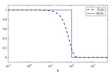
Figure 1 plots the Gaussian kernel in -space and compares it to sharp-spectral truncation. Note that a Fourier analysis is not possible in the non-homogeneous (vertical) direction. A detailed discussion on the different kernels can be found in Rivera et al. (2014) (see Figures 12, 13 in that paper and associated discussion). The Gaussian kernel form in equation (7) has been used in several prior studies (Piomelli et al., 1991; Wang et al., 2018) due to its numerical discretization advantages (see John (2012), page 30).
In simulations with non-periodic boundary conditions, such as our RT flow with rigid walls at the top and bottom, filtering near the boundary requires a choice for the fields beyond the boundary. In this paper, the choice is to extend the domain beyond the physical boundaries with values compatible with the boundary conditions (Aluie et al., 2018). Filtering near the wall is then performed on this extended data. For our RT problem specifically, the velocity is kept zero beyond the walls, the density field is kept constant (zero normal gradient), and the extended pressure field satisfies the hydrostatic condition . The coarse-graining operation can then be performed at every point in the flow domain without requiring complicated inhomogeneous filters, which do not commute with spatial derivatives.
Analyzing the energy cascade and inertial range dynamics in constant-density turbulence centers on studying the large scale kinetic energy (KE), . Since KE in variable density flows, , is non-quadratic, its large scale definition is not as straightforward. Several different definitions have been proposed in the literature, including (Chassaing, 1985; Bodony & Lele, 2005; Burton, 2011; Karimi & Girimaji, 2017), and (Kida & Orszag, 1990; Cook & Zhou, 2002; Wang et al., 2018). However, as was shown in Zhao & Aluie (2018), the above two definitions can fail to satisfy the ‘inviscid criterion’ in flows with large density variations, leading to viscous contamination at all scales, and preventing the unravelling of inertial range dynamics. The ‘inviscid criterion’ requires that viscous contributions be negligible at large scales. Aluie (2013) proved mathematically, and Zhao & Aluie (2018) showed numerically, that the Favre decomposition, , where
| (9) |
is the Favre filtered velocity (Favre et al., 1958; Aluie, 2013; Eyink & Drivas, 2018), satisfies the inviscid criterion even in the presence of arbitrarily large density variations. In the current paper, we shall adopt the Favre decomposition when analyzing scale dynamics.
2.4 Simulation results
| Label | Grid size | |||||||||
|---|---|---|---|---|---|---|---|---|---|---|
| 3D1024 | 3.2 | 3.2 | 6.4 | 0.5 | 15.07 | 13854 | 0.70 | 0.45 | ||
| 3D512high | 1.6 | 1.6 | 3.2 | 0.8 | 7.44 | 4582 | 0.80 | 0.28 | ||
| 3D512low | 3.2 | 3.2 | 6.4 | 0.15 | 27.38 | 8027 | 0.49 | 0.55 | ||
| 2D4096 | 3.2 | – | 6.4 | 0.5 | 0.94 | 44562 | 2.25 | 0.45 | ||
| 2D2048high | 3.2 | – | 6.4 | 0.8 | 0.93 | 25766 | 2.36 | 0.39 | ||
| 2D2048low | 3.2 | – | 6.4 | 0.15 | 0.43 | 12397 | 2.99 | 0.55 | ||
| 2D2048 | 3.2 | – | 6.4 | 0.5 | 7.53 | 44052 | 0.52 | 0.45 | ||
| 2D1024 | 3.2 | – | 6.4 | 0.5 | 60.3 | 38002 | 0.28 | 0.45 | ||
| 2D1024lowM | 3.2 | – | 6.4 | 0.5 | 59.38 | 41949 | 0.26 | 0.13 |
Two- and three- dimensional Rayleigh-Taylor simulations are performed to analyze the energy budget and cascade in RT turbulence. These simulations, summarized in Table 1 are performed at low and high Atwood numbers, with grid resolution up to in 2D and in 3D. The Atwood number is defined by , where are the densities of the initial uniform heavy and light fluids. The results shown below are primarily based on the largest simulations 2D4096 and 3D1024, while other simulations shown in the table are for numerical convergence and verification purposes.
The initial conditions for simulations shown in Table 1 are as follows. Initial density field is composed of uniform heavy fluid on top with , and uniform light fluid with density at bottom. The initial pressure field satisfies hydrostatic balance , with pressure at bottom set to be 10 for all simulations in Table 1, except 2D1024lowM, where pressure is set to 100 at the bottom to yield lower compressibility levels. In Appendices A, we show that our results do not depend on the compressibility level of RT flows. The velocity fields are initially zero with perturbations added to the interface of vertical velocity. The interfacial velocity perturbations are imposed in wavenumber space, and are nonzero only within a band of high wavenumbers. In 3D, the velocity amplitude is perturbed in a shell , and the magnitude is set to be proportional to , where is a normalization constant to further limit the range of effectively perturbed wavenumber. While in 2D, the velocity amplitude is perturbed in an annulus , with magnitude proportional to , where is the same constant as in 3D. Since the perturbation wavenumber band is slightly different between 2D4096 and 3D1024, for verification purpose, we also perform additional 2D simulations 2D1024 and 2D2048 (see Table 1) with initial perturbations identical to those in 3D1024. Analysis results based on these 2D simulations are similar to the 2D4096 case, and are shown in the Supplementary Material, section D.
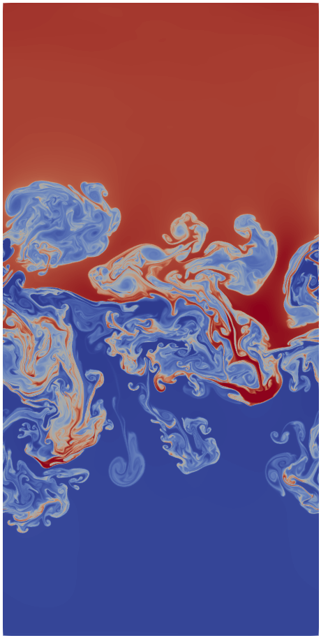
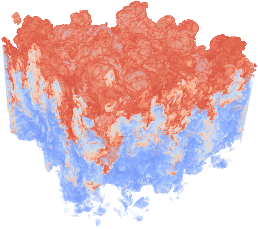
Visualizations of density snapshots are shown in figure 2(a) for the 2D4096 case and figure 2(b) for the 3D1024 case, both at dimensionless time , where is the characteristic time scale, and is the gravitational acceleration. Both figures show complex flow patterns and structures with a wide spectrum of sizes. It is also easy to see that the 3D field develops much finer scale structures than the 2D field, a property which we will quantify using spectra below. We now present some basic properties of our simulations.
2.5 Mixing width
The mixing width is an important quantity characterizing the total width of the mixing layer between bubble and spike fronts in RT flows. It is used to quantify the penetration depth of RT bubbles and spikes into the unperturbed flow. When there are sufficient multimode interactions, turbulent RT flows become self-similar at later times (Birkhoff, 1955; Ristorcelli & Clark, 2004; Dimonte et al., 2004). During the self-similar stage, the mixing width is well-described by , a quadratic growth in time which is proportional to a constant coefficient .
The value for has been the subject of vigorous research and discussion within the community. It is believed to depend on whether initial conditions render the RT flow in the bubble competition regime or in the bubble merger regime (e.g. Ramaprabhu et al., 2005). Numerical simulations of 3D-RT in the bubble merger regime generally report values to (see Table 6.1 in Zhou (2017a) for a summary), although values larger than have been reported in 3D simulations using front tracking (e.g. Glimm et al., 2013). Experiments on the other hand generally report much larger values to (Zhou, 2017a), which is thought to be a result of unintended large-scale perturbations (Dimonte et al., 2004).
While we report values from our simulations here, its precise value is far from being the focus of our paper. Our interest in here is rather more limited to comparing its values from 2D simulations relative to 3D simulation within the same modeling framework. For reasons that remain unclear and subject to various speculations, the parameter in 2D simulations has often been found larger than in 3D simulations (e.g. Youngs, 1991, 1994; Dimonte et al., 2004; Cabot, 2006). Such enhanced RT growth in 2D simulations has been somewhat of a puzzle given that both analytical models and simulations of single-mode RT predict that it is growth in 3D that should be faster (Layzer, 1955; Goncharov, 2002; Bian et al., 2020). A goal of this paper is to shed light on the puzzle.
We calculate the mixing width using the formula (Cabot & Cook, 2006; Zhang et al., 2018b):
where denotes a horizontal average of the density field, which is a function of and , and denote the original heavy and light fluid densities.
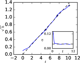
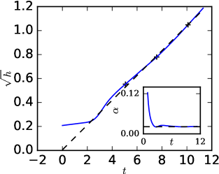
After obtaining , can be calculated using one of two methods. The first is by directly calculating , while the second is by carrying a best linear fit between and in the self-similar regime (Olson & Jacobs, 2009). Figure 3 plots versus time from the 2D4096 and 3D1024 data, and a linear fit in the self-similar regime is marked with a dashed line. The inset of the figures corresponds to the first approach: is plotted against time, while the value obtained by the linear fit is marked with a horizontal dashed line. We obtain the same results from these two methods. Figure 3 shows that there is a substantial time range of self-similarity in both 2D and 3D, in which there is an excellent linear fit between and . The values of we obtain (0.036 in 2D and 0.021 in 3D) fall within the range reported from simulations in the literature (Cabot & Cook, 2006; Dimonte et al., 2004). Note that from the 2D-RT is almost twice as large as that from 3D-RT.
2.6 Overall energy balance
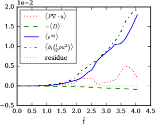
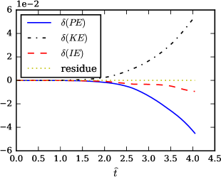
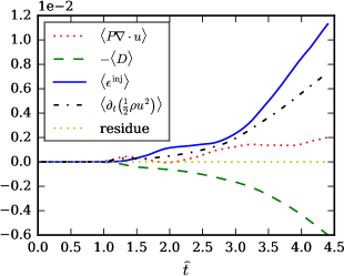
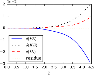
We shall now discuss the bulk balance between potential energy, kinetic energy, and internal energy in our simulated flows. Temporal evolution of the spatial mean of each of the budget terms in the kinetic energy equation (5) is shown in figures 4(a) and 4(c) for 2D and 3D, where is the dissipation term, and is the energy injection. Correspondingly, figures 4(b) and 4(d) show the temporal evolution of bulk (over volume of the domain) potential energy , bulk internal energy , and bulk kinetic energy , in 2D and 3D. The bulk energy is measured relative to its initial value:
| (10) | |||||
| (11) | |||||
| (12) |
The second equality in equation (10) is due to the relation (Cabot & Cook, 2006), while equation (11) can be obtained by time integrating the internal energy equation (4).
Plot of 2D instantaneous energy budget terms in figure 4(a) shows the time derivative of kinetic energy and the energy injection rate keep increasing in time, while the average value of is positive so that internal energy is converted to kinetic energy via this term. The overall viscous dissipation term is negative and converts kinetic energy to internal, but the amount of conversion is smaller in magnitude relative to in 2D. Thus, in figure 4(b) both the overall internal energy and potential energy decrease and are converted to kinetic energy. The overall bulk energy balance satisfies , as is marked by the ‘residue’ term in the figure.
The corresponding 3D results are shown in figures 4(c) and 4(d). The injection rate and time derivative of KE keeps increasing, while the dissipation and pressure dilatation terms convert between kinetic and internal energy. One difference from 2D is that in 3D, the dissipation term contributes more than , and the overall energy conversion is from kinetic to internal, opposite to the 2D case. Total energy conservation, , still holds in 3D. This conservation holds in all simulations in Table 1. In section 3, we will present a more refined balance relation applied to the coarse-grained quantities, where the balance of energy at different length scales is established.
The rate-governing quantities in our figure 4 seem more sensitive to fluctuations around the self-similar trajectory than the mixing width in figure 3, which has often been the main focus of previous RT studies. The fluctuations may be either due to intrinsic variability or due to a transient response to initial conditions, the removal of which has been recently discussed in Horne & Lawrie (2020). That figure 16 in the Appendix shows similar fluctuations under different initial and compressibility conditions suggests it may be the former, yet a careful investigation of this observation is beyond the scope of our paper. Nevertheless, we shall show below that energy transfer across scales exhibit clear self-similar evolution despite the presence of these fluctuations in the rate-governing quantities.
One may notice that mean injection, , shown in figures 4(a) and 4(c), grows more rapidly in 2D than in 3D. There are two (related) ways to understand this: (i) the mixing width growth rate in 2D is larger than in 3D and, thus, the mixing layer width should be larger in 2D than in 3D at any physical time. This implies that relatively more potential energy is released in 2D due to the rising light fluid and sinking heavy fluid, leading to a higher mean injection . (ii) From the balance relation , we have in 2D, which is converted to kinetic energy, while in 3D. This implies a larger mean kinetic energy is expected in 2D, and thus is expected to be larger in 2D than in 3D. This leads to a larger in 2D. We shall show below that there is a deeper physical explanation behind these differences between 2D and 3D RT arising from differences in the energy pathways across scales. Given the difference in between the RT flows in 2D and 3D, we shall normalize by it to allow for a fair comparison of the budget terms between 2D and 3D.
2.7 ‘Filtering’ spectra
For completeness, we now present the spectra of density, velocity, and kinetic energy using our RT data. In homogeneous constant-density flows, the energy spectrum is obtained by taking the Fourier transform of the velocity field and summing over shells in wavenumber space: . Obtaining the spectra for variable density RT flows is difficult because i) the domain is not periodic in the vertical direction so the Fourier transform is not straightforward, and ii) the non-quadratic nonlinearity of kinetic energy poses another problem.
Previous works in RT (Cook & Zhou, 2002; Cabot et al., 2004) obtained the spectra for density and velocity by Fourier transforming in the horizontal periodic directions and then taking an average in the vertical direction. By taking Fourier transforms only in the horizontal directions, spectral information in the vertical direction is completely ignored.
Unlike in constant density turbulence, where the spectrum of energy is the same as that of velocity, in variable density the two quantities are different. Moreover, when kinetic energy is non-quadratic, there are many possible ways to construct a “spectrum” in -space having units of energy per wavenumber. These different “energy spectra” correspond to the Fourier transform (or scale decomposition) of different combinations of variables and are not equivalent. To avoid the difficulty pertaining to its non-quadratic nature, previous studies constructed a kinetic energy spectrum by introducing a new variable and analyzing it in Fourier space, . However, as emphasized in Zhao & Aluie (2018), the evolution of is fundamentally different from the evolution of momentum, , especially when each of these variables is being decomposed in scale. A length-scale does not exists on its own but is associated with the variable being decomposed. Zhao & Aluie (2018) showed that this new variable fails to satisfy the ‘inviscid criterion’ in variable density flows, which means that dissipation can contaminate its large scale dynamics in the presence of significant density variations. Thus, is not an appropriate quantity to analyze because it is inconsistent with inertial-range dynamics. Moreover, as was observed in Zhao & Aluie (2018), a putative power-law scaling of a quantity alone, such as , is not indicative of an inertial cascade (see Supplementary Material, section C).
Here we adopt a new approach to obtain the spectra using spatial coarse-graining. For any field , the filtering spectrum is defined as (Sadek & Aluie, 2018):
| (13) |
where , is the domain size of interest, is the scale we are probing, and stands for spatial averaging. The filtering spectrum of kinetic energy is
| (14) |
Sadek & Aluie (2018) showed that this filtering spectrum guarantees energy conservation, similar to the Plancherel theorem when working with Fourier spectra. The filtering spectrum allows us to measure the energy content at scale by probing the change in as is varied. The calculation can be done in physical space without any Fourier transforms. The obvious advantage is that definition (13) allows us to extract the spectrum in inhomogeneous flows such as RT. Moreover, the filtering spectrum generalizes easily to non-quadratic quantities, such as kinetic energy, , in variable density flows. The Fourier spectrum, on the other hand, is limited to quadratic quantities and requires treating kinetic energy as such, even when this is inconsistent with the dynamics.
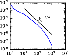
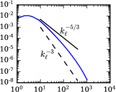
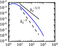
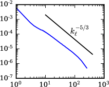
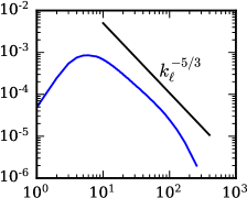
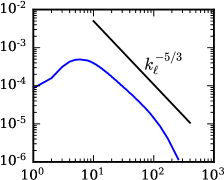
Figure 5 shows the spectra of density, velocity, and kinetic energy for 2D and 3D RT flows calculated with the above definition. The density spectra follow a putative scaling over an intermediate wavenumber range in both 2D and 3D. The velocity spectrum in 2D is steeper than but shallower than as would have been expected from 2D homogeneous constant-density turbulence (e.g. Boffetta & Ecke, 2012). In 3D the filtering spectrum is slightly shallower than a scaling over a decade. The kinetic energy spectra follow similar scalings as the velocity field. Both velocity and kinetic energy spectra attain a peak value at low wavenumbers, where most of the energy content resides. In contrast, the density spectra show the importance of much larger scales due to density variation in the vertical. Indeed, the density jumps between heavy and light fluids is expected to yield a spectrum , which is consistent with the scaling at the largest scales. Plots in figure 5 demonstrate the utility of the coarse-graining approach to probe the spectral content in all directions, including scales along the inhomogeneous (vertical) direction, as discussed in Sadek & Aluie (2018). For completeness, we show in the Supplementary Material section C the filtering spectra for three different scale decompositions of kinetic energy.
3 Multi-scale energy balance in RT flows
We now investigate the energy scale pathways of Rayleigh-Taylor flows. We employ the Favre decomposition as discussed in sections 2.3 and 2.7 to chart the channels for potential energy, internal energy, and kinetic energy at large and small scales. Energy conversion between different forms and across different length scales is investigated by analyzing the budget terms from numerical data.
3.1 Coarse-grained energy budget equations
Within the Favre decomposition, the budgets for large and small scale kinetic energy, internal energy, and potential energy are:
| (15) | ||||
| (16) | ||||
| (17) | ||||
| (18) |
where is specific internal energy, is potential energy density, is spatial transport of kinetic energy, and are kinetic energy fluxes across scale , is large scale pressure dilatation, is viscous dissipation, and is KE injection (hence, the ‘inj’ superscript) due to gravity at scales larger than . These terms are defined as:
| (19) | ||||
in which is the generalized 2nd order moment (Germano, 1992): and . Note that our small scale kinetic energy, defined as , is sometimes referred to as ‘subscale’ or ‘subgrid’ kinetic energy in the LES literature.
Coarse-grained potential energy density equation (18) can be derived by noting that
We analyze the energy pathways by inspecting the budget equations (15)-(18) using our simulations in Table 1. In particular, we shall demonstrate the existence of an inertial range in such flows. Note that we do not formulate budgets for small scale internal energy and potential energy, since it is unclear if these two quantities cascade (Eyink & Drivas, 2018).
3.2 Energy pathways in RT flows
This section presents some of the main results of our paper, which we summarize in Section 3.2.5 for the reader’s convenience. Here, we refine our analysis of the global energy balances in figure 4 at different scales via coarse-grained budgets. The types of energy involved in the scale-transfer, as shown in equations (15)-(18), are potential energy, internal energy, large scale kinetic energy, and also small scale kinetic energy. Differences in the energy pathways between 2D and 3D will be emphasized during our presentation.
3.2.1 Conversion between different forms of energy
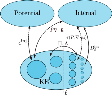
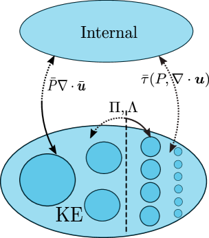
Figure 6 summarizes the RT energy pathways we discuss in this section. In RT flows, the ultimate energy source is the release of potential energy from the initial unstable density stratification. From equation (18), large scale potential energy is a source for large scale kinetic energy via in equation (15). Small scale kinetic energy injection is identically zero for RT flows since the gravitational acceleration is constant in space. Thus, potential energy is available directly to large scale kinetic energy. Meanwhile, kinetic energy is also linked to internal energy via pressure dilatation and viscous dissipation. The term appears as a source in large scale KE equation (15) and a corresponding term is a source in small scale KE budget equation (16), while both appear as sinks in the internal energy equation (17). Similarly, dissipation terms and are sinks in large and small scale KE budgets, respectively, and sources in the internal energy budget: . These channels, summarized in figure 6, are responsible for converting energy between different forms. In addition to these conversion channels, the transfer between large and small scale kinetic energy is now presented.
3.2.2 Kinetic energy scale pathways
There are two kinetic energy fluxes across scales, and . Deformation work is solely due to the turbulent velocity field, which is closely related to vortex stretching in constant-density 3D turbulence (e.g. Eyink, 2006). Baropycnal work was shown in Lees & Aluie (2019) to transfer energy by strain and vorticity generation, in which density, pressure, and velocity fields all play a role. These fluxes provide a pathway for kinetic energy across scales, and operate in the ‘inertial range’, as we shall see shortly.
Figure 6 sketches the mean or bulk pathways based on the energy budgets. Some arrows in the schematic are dashed, representing energy transfer directions which are not realized dynamically in our RT flows. For example, gravity converts potential energy to large scale KE despite the kinematic possibility for the transfer to be in reverse. Pressure dilatation converts internal energy to large scale KE. Baropycnal work, , transfers energy from large-scale KE to smaller scales, consistent with its role as as an energy flux. Deformation work, , also transfers KE energy downscale, but only in 3D. We find that transfers KE in the reverse direction in 2D, from small to large scales. However, the total flux is always downscale in both 2D and 3D. Irreversible viscous dissipation converts only small-scale (but not large-scale) KE to internal energy due to our scale-decomposition satisfying the inviscid criterion. Last, although mean is a kinematically possible pathway between small scale KE and internal energy, we observe it is close to zero in our RT flows. This is consistent with previous studies showing that mean pressure dilatation is a large-scale process and does not couple kinetic and internal energy at small scales, on average (Aluie, 2011; Aluie et al., 2012; Kritsuk et al., 2013; Wang et al., 2013).
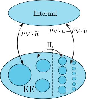
Note that in the LES modeling literature, another formulation of the kinetic energy budget is often used in which baropycnal work, , is missing by lumping it with pressure dilatation. The traditional LES formulation is mathematically equivalent to our equation (15), but the physical interpretation of energy pathways is different. Stated briefly, our KE budget allows for an inertial range over which kinetic energy can cascade (Aluie, 2011, 2013), unlike the more common LES formulation, which misses the distinct physics of baropycnal work that is essential in variable density flows such as RT. A discussion is presented in Supplementary Material, section E.
3.2.3 The inertial range in turbulent RT flows
Having identified the pathways, we now present a quantitative analysis. We calculate all terms in the large scale kinetic energy budget (15) as a function of scale , which allows us to test and validate ideas on energy conversion and the cascade.
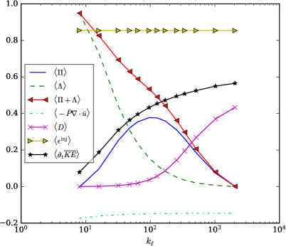
The results from the 2D4096 simulation (see Table 1) are shown in figure 7, while the 3D1024 results are in figure 8. These figures plot the domain averaged terms in equation (15) as a function of filtering wavenumber (inverse of scale) . Note that our “filtering wavenumber” does not involve any Fourier transform, and we only use it to refer to the corresponding scales, as is conventional in the turbulence literature. For large (small scales), these terms approach their unfiltered values. Therefore, they represent cumulative processes acting at all scales larger than and not just the contribution from scale itself. For example, if increases in value over the range (), then the KE content of scales within the band is growing. The only exceptions are the flux terms, and , which are hybrid quantities involving coarse-grained fields ( or ) acting against subscale contributions ( or ) and, therefore, represent the energy transfer across the partitioning scale (Aluie, 2011, 2013).
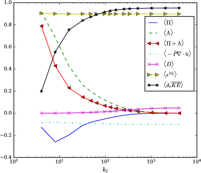
Figures 7, 8 show results from the 2D4096 and 3D1024 simulations, respectively. Spatial mean injection shown in the figures is constant in , which is due to the spatially uniform gravitational acceleration used here (Aluie, 2013). The reason becomes clear when considering that is independent of . This implies that mean injection from potential energy is released directly only at the largest scale (Aluie, 2013). To elaborate, consider two scales, one with length , the largest in the system, and another with a smaller length scale . Since mean injection at the two distinct scales are the same, injection within the band of scales is zero. Taking the limit , it is obvious that no mean injection occurs at any scale below . Thus, mean injection occurs only at the largest length scale, that of the domain size. Subsequent transfer to smaller scales occurs via the fluxes and , as we shall discuss below.
Similar to injection, mean pressure dilatation is almost flat as a function of in figures 7, 8. This is consistent with predictions in Aluie (2011) and simulations by Aluie et al. (2012), where the pressure dilatation was shown to operate over a transitional scale range of limited extent. Hence, mean pressure dilatation only affects the large scale dynamics. Dissipation within the Favre scale decomposition has already been proved to be negligible at large scales (Aluie, 2013; Zhao & Aluie, 2018), which is again confirmed here in figures 7, 8. Thus, in well developed RT turbulence, there is a range of length scales which is immune from injection and pressure dilatation at large scales, and also from dissipation at small scales. This range of length scales is the ‘inertial range’ in the spirit of Kolmogorov’s turbulence theory. Within this inertial range, kinetic energy dynamics is governed by the two fluxes and .
3.2.4 Energy fluxes across scales
The narrative that will emerge throughout this paper indicates that baropycnal work, , in RT flows acts as a conduit for gravitational potential energy, transferring (non-locally in scale) the energy deposited by at scale to smaller scales. Figures 7,8 show that is positive, acting as a KE source for intermediate to small scales. Mean decays monotonically with in both 2D and 3D, indicating that does not persist to arbitrarily small scales. As we discuss in Supplementary Material, section A, this decay is consistent with being predominantly a non-local transfer in scale. As shown in figures 7,8, the decrease in is accompanied by an increase in at those scales. This implies that as RT turbulence is evolving, acts as a KE source for unsteady scales within the inertial range, increasing their KE content. The largest scales increase their KE content the most, leaving less energy to be transferred by to smaller inertial scales, which explains why is not persistent (i.e. constant) but decays with smaller . Further analysis of ’s scale-locality and decay in is undertaken in Supplementary Material, section A.
As these inertial scales become energetic enough and vortex stretching starts operating in 3D (figure 8), deformation work takes over and transfers energy to smaller inertial scales similar to constant-density homogeneous 3D turbulence. Transfer by is strongest (peak in figure 8) at an inertial scale that grows in time and is smaller than the mixing width. In the absence of vortex stretching in 2D (figure 7), is negative as in constant-density homogeneous 2D turbulence, transferring energy upscale. Hence, the only mechanism for growth of small scale kinetic energy in 2D is baropycnal work .
The downscale cascade of energy by in 3D delivers energy to viscous scales which is manifested by large values of viscous dissipation in figure 8. In contrast, dissipation levels in 2D are miniscule since , cascading energy upscale. This fundamental difference also explains the difference in spectra in figure 5, where there is less energy at small scales () in 2D relative to 3D, despite there being more overall KE (integrated across all scales) in 2D relative to 3D. This is because in 3D acts as a source term for these small inertial scales, in addition to , delaying the saturation of KE at these scales in 3D relative to 2D.
Indeed, note that as a function of scale in 2D in figure 7 saturates to a constant value at , with almost zero KE growth at higher . This indicates that at the time being analyzed, these small scales have reached a steady state and are not increasing on average. However, in 2D, unlike in 3D, their energy is subsequently transferred to large scales by (which is negative), resulting in a low level of dissipation of kinetic energy. In contrast, and are both positive in 3D, transferring a larger amount of energy to small scales compared to 2D. This leads to higher KE levels at small scales in 3D, as evidenced by plots of spectra in figure 5 and also of in figure 8, which keeps increasing as a function of , indicating that those scales are still growing and have not yet reached a steady state. Since viscous dissipation is most effective at the smallest scales (within the Favre decomposition), this substantially higher energy input at high in 3D (versus 2D) leads to the higher levels of energy dissipation in figure 8 (versus figure 7).
Our analysis points to fundamental differences in physics between 2D and 3D RT instabilities. It is often observed that the turbulent RT instability mixing layer grows faster in 2D simulations relative to 3D simulations111It is worth noting that Horne & Lawrie (2020) have reported smaller in quasi-2D RT experiments. However, Ekman friction is prominent as discussed lucidly in that work and it would be expected to reduce the value since it acts preferentially on large-scales.. This is captured by the parameter appearing in the mixing width evolution, , which has often been found to be larger in 2D than in 3D (Youngs, 1991, 1994; Dimonte et al., 2004; Cabot, 2006), consistent with the values we found in figure 3. The enhanced growth in 2D simulations has been somewhat of a puzzle since single-mode (non-turbulent) RT instability models and simulations predict that it is growth in 3D that should be faster (Layzer, 1955; Goncharov, 2002; Bian et al., 2020). The difference in values in turbulent RT instability had been attributed to the smaller dissipation levels in 2D (Youngs, 1991, 1994), although we have seen above that viscous dissipation levels are merely a symptom (or a consequence) of the energy scale-fluxes and do not directly influence inertial-range dynamics governing the mixing layer.
The fundamental difference in inertial-range physics is that deformation work channels energy upscale in 2D and downscale in 3D. In 2D-RT, redirects energy delivered by to inertial scales back to larger scales, driving a positive feedback loop that is absent in 3D-RT. In this feedback loop, the upscale cascade leads to an enhanced growth of the mixing layer, which in turn leads to enhanced potential energy release (as seen in figure 4) by raising the light fluid and lowering the heavy fluid. The excess release of potential energy results in enhanced baropycnal energy transfer by to smaller scales which is re-channeled back upscale by , closing the feedback loop. This narrative is consistent with plots of filtering spectra in figure 5, where we see that the KE (and velocity) spectral peak in 2D is at larger scales and has a higher magnitude compared to 3D. Cabot (2006) had speculated that the difference in between 2D and 3D may be due to an inverse energy cascade in 2D-RT, although that study did not conduct an analysis of energy transfer across scales. Our results here provide thorough evidence in support of that hypothesis, and highlight the potentially misleading 2D-RT flow physics when modeling real-world 3D-RT flows.
Another important conclusion we can draw from our analysis is the absence of a net upscale energy transfer in 3D-RT. In many studies discussing RT flows in 3D, motivated by ICF (e.g. Shvarts et al. (1995); Alon et al. (1995); Ofer et al. (1996); Oron et al. (2001); Zhou et al. (2003)), or astrophysics (e.g. Joggerst et al. (2010); Porth et al. (2014)), or fundamental fluid dynamics (e.g. Abarzhi (1998); Cheng et al. (2002); Cabot (2006)), it is often claimed that the generation of successively larger bubbles following the presence of smaller ones is due to an inverse cascade of energy which causes small bubbles to merge into larger ones. According to such a narrative, the small-scales are the source of energy feeding and sustaining the large-scales, even in 3D.
Such claims are often based on qualitative observations of the flow development, including spectral energy content, but without clarifying the causality of energy spectral broadening and do not analyze the energy transfer across scales directly (e.g. scale fluxes and ) as we do here. While energy at small scales saturates before energy at larger scales, this does not necessarily imply that energy is being continuously channelled to the small-scales and back up to larger scales. Indeed, our findings indicate the absence of a net upscale energy transfer in 3D-RT, and that growth of large-scale bubbles and spikes is solely due to baropycnal work in 3D, which deposits energy directly from gravitational potential energy at the largest scales in the system. No persistent upscale transfer of energy is required222Beating of modes to seed larger scales from smaller ones can still transfer minuscule amounts of energy upscale but this is fundamentally different from the notion of a cascade, which requires persistent transfer in scale and/or time. Consider, for example, 3D constant-density homogeneous isotropic turbulence (HIT) forced at an intermediate wavenumber in a triply periodic domain and having slightly smaller wavenumbers gain finite energy. Such transient upscale energy transfer is not sustained (or persistent) in wavenumber, which is why it is widely agreed that an inverse cascade in 3D-HIT is absent. Another example is the downscale cascade of enstrophy in 2D constant-density flows: there is invariably non-zero energy transferred downscale along with enstrophy, but such energy transfer is not a cascade since it is not persistent in scale, vanishing rapidly as within the inertial range (Kraichnan, 1967). to explain the evolution of spectral energy content. The assumed existence of an inverse cascade had been used in some instances (e.g. Abarzhi, 1998) to explain the dependence of RT flows on initial perturbations (Dimonte, 2004; Ramaprabhu et al., 2005). If this were the case, it would have created significant difficulties in the subgrid modeling of RT flows. Our results here provide compelling evidence that the inverse cascade narrative in 3D-RT is unjustified.
3.2.5 Summary of RT energy pathways
Section 3.2 presented some of the main results of this paper, which we now summarize. We showed that Baropycnal work, , in RT flows acts as a conduit for gravitational potential energy, transferring the energy deposited by at the largest domain scale to smaller scales. As these inertial scales become energetic enough and vortex stretching starts operating in 3D (figure 8), deformation work takes over and transfers energy to smaller inertial scales. The net downscale cascade of energy by in 3D delivers energy to viscous scales which is manifested by large values of viscous dissipation. In contrast, in 2D-RT, redirects energy delivered by back to larger scales via an upscale cascade. The upscale cascade in 2D leads to an earlier saturation of small inertial scales compared to 3D, which explains why small inertial scales are weaker than in 3D (see spectrum in figure 5). This is despite the greater overall KE (integrated across all scales) in 2D relative to 3D, which is explained by the positive feedback loop in 2D-RT.
The upscale cascade in 2D-RT drives a positive feedback loop that is absent in 3D-RT. In this feedback loop, the upscale cascade leads to an enhanced growth of the mixing layer, which in turn leads to enhanced potential energy release (as seen in figure 4) by raising the light fluid and lowering the heavy fluid. The excess PE released results in enhanced baropycnal energy transfer by to smaller scales which is re-channeled back upscale by , closing the feedback loop.
3.3 Spatial distribution of fluxes
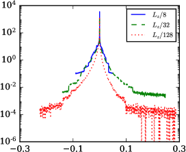
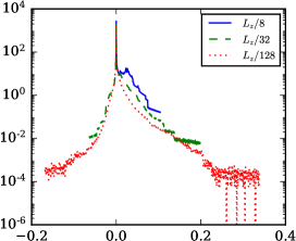
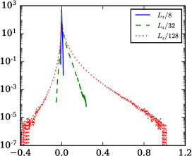
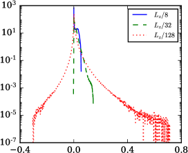
The spatial distribution of values for fluxes and is shown by their PDFs in figure 9, for 2D and 3D RT. Results at three scales are shown. All PDFs are non-Gaussian, with heavy tails and a stronger departure from Gaussianity at smaller scales. In 2D, is skewed towards negative values, but in 3D it is positively skewed, reflecting the inverse versus forward net energy cascade by in 2D versus 3D. The PDF of is always skewed towards positive values. In particular, at large scales (e.g., ), is positive everywhere in the domain as is seen in figures 9(b) and 9(d). As we shall discuss in Zhao et al. (in preparation), negative values of are correlated with spiraling regions of the flow, which are part of the mushroom structure that appears in late time single-mode RT. Note that the PDF of in 2D (figure 9(b)) contains both positive and negative values when is below or equal to , while the PDF of in 3D (figure 9(d)) is almost always positive even at . This observation is in accord with visualizations of density fields in figures 2(a) and 2(b) where 3D-RT exhibits much finer structures than in 2D-RT, such that the spiraling structures are on average smaller in 3D.
3.4 Temporal self-similarity of flux terms
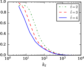
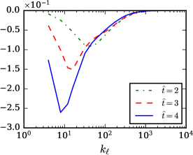
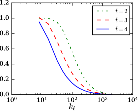
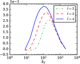
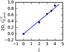
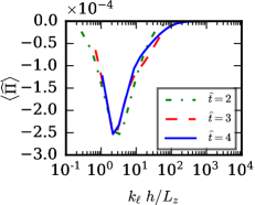
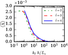
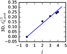
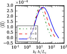
So far, we have discussed the fluxes as a function of scale at one time instant. In this section we investigate their temporal evolution. Figure 10 shows mean and normalized by at dimensionless times using the 2D4096 and 3D1024 RT data (see Table 1). As RT turbulence develops, the magnitude of normalized decreases, whereas the normalized increases in magnitude. Note, however, that the absolute values of both fluxes keep increasing (not shown). A decrease in normalized indicates that as KE at scale saturates in time, the relative importance of , which is responsible for redistributing injected energy from the potential release, also decreases. In contrast, turbulence levels in RT flows increase in time, leading to an increasing relative magnitude of . The scale corresponding to the peak magnitude of , indicated by , shifts to smaller (or larger scales) over time. For example, in 2D, shifts from at , to at , while in 3D, shifts from about at to at . Thus, as expected, turbulence encroaches onto larger scales as RT evolves, so that vortex stretching (in 3D) or mergers (in 2D) which drive the flux are more pronounced at these scales.
The above observations indicate possible self-similar (in time) behavior of turbulent RT fluxes. If we plot the scales corresponding to the peak magnitude of , which we denote as , against dimensionless time , we obtain a quadratic scaling in time as shown in figures 11(a),(d), similar to the mixing width in figure 3. Figures 11(a), (d) indicate that, in both 2D and 3D, , with the coefficients
| (20) |
where are the mixing widths from the 2D4096 and 3D1024 RT data. Note from figure 10 (also figures 11(b),(e)) how in 2D is skewed to larger scales, unlike in 3D, peaking at approximately half the size of the mixing width, (equation (20)). This is consistent with the net upscale transfer by driving the mixing layer growth as discussed in section 3.2.4. In comparison, in 3D is symmetric, peaking at a scale smaller than the mixing width, .
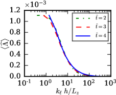
The temporal scaling of in figures 11(a),(d) is evidence that the evolution of mean fluxes is self-similar. Recall that self-similarity implies that functions of length and time, such as and , should collapse to the same curve when properly rescaled (Ristorcelli & Clark, 2004). Specifically, the rescaled fluxes should satisfy
| (21) | ||||
where is just filtering wavenumber , rescaled by the mixing width , . , are temporal scaling functions, and are the similarity functions. If mean fluxes are temporally self-similar, then should collapse onto the same curve.
Figures 11(b),(e) for in 2D and 3D, and figures 11(c),(f) for in 2D and 3D indicate that they indeed collapse onto each other. In figures 11(b),(e), the horizontal axis is rescaled by the mixing width . To account for the temporal function , we rescaled the plots at so that their maxima match with that at . The same rescaling amplitudes for are also applied to , as is shown in figures 11(c),(f), which indicates that . We have found that and follow a scaling close to both in 2D and 3D (not shown). This growth of the fluxes can be understood from the cumulative amount of potential energy released, which follows (Dimonte et al., 2004), implying that the rate of kinetic energy injection should scale as . This energy is eventually channeled by the fluxes and , which grow in magnitude accordingly.
While plots of the fluxes show good collapse in figure 11, it is worth discussing the relatively poor collapse of in 3D (figure 11(e)) at scales smaller than that of the peak. The reason decays at those scales is due to viscous dissipation removing the kinetic energy available to cascade. As the RT flow evolves and there is more kinetic energy cascading, the dissipation scale should become smaller as as shown in Ristorcelli & Clark (2004) by invoking Kolmogorov’s turbulence phenomenology. This is reflected in extending to smaller scales at later times in figure 11(e). Therefore, the dissipation dynamics is not expected to follow the temporal self-similarity of inertial scales captured in equation (21). Note that the cascade in 2D, being upscale, is not arrested by viscous dissipation at the smallest scales, which explains the much better collapse of in figure 11(b).
(a)
(b)
(c)
(d)
(e)
(f)
4 Directionally split analysis of RT anisotropy
In RT flows the kinetic energy injection acts only in the vertical direction due to the downward gravitational acceleration. In addition, the initial and boundary conditions are different in the horizontal and vertical directions. Therefore, anisotropy both in the bulk flow and as a function of scale is expected in RT flows. Using DNS data, Cabot & Zhou (2013) examined RT anisotropy mostly based on bulk flow quantities such as the Taylor microscale, Kolmogorov scale, and velocity derivatives, and using other statistical measures such as correlation functions. These quantities do not rely on a proper scale decomposition. They also analyzed anisotropy as a function of scale but only in the homogeneous directions using Fourier transforms to measure spectra. They found that large scale dynamics (based on the bulk flow and Fourier spectra) in RT is highly anisotropic, but that the flow becomes more isotropic at small scales, where velocity derivatives appear more isotropic than the velocity field itself. In a follow-up work, Zhou & Cabot (2019) studied the time evolution of anisotropy, mixing, and scaling in RT instability, extending their previous one-snapshot analysis to different times and Atwood numbers. Other works on anisotropy of RT relied on analyzing the normalized deviatoric part of the Reynolds stress tensor, to measure the anisotropy in RT flows (Livescu et al., 2009, 2010; Banerjee et al., 2010; Zhou, 2017b), whose values are bounded between and . Nonzero values of indicate deviation from isotropy, and typical values of or are observed with DNS RT data (e.g. Livescu et al., 2009). The above works relied primarily on statistical approaches, such as Reynolds averaging, to analyze RT anisotropy, which are not capable of identifying anisotropy as a function of scale. On the other hand, a Fourier scale decomposition is limited to homogeneous (horizontal) directions. A more refined analysis is possible with our coarse-graining approach, which analyzes the scale-by-scale anisotropy in RT flows, as we shall discuss now and also in Supplementary Material, section B.
4.1 Directionally split anisotropy at scales
Here, we investigate anisotropy of RT flows at different scales in physical space. To quantify the contribution to the kinetic energy budget from different directions, we first formulate the budgets along each direction separately, and then diagnose the constituent terms from numerical data. We call this ‘directionally split’ analysis of anisotropy, which is different from the analysis of scale anisotropy done in Supplementary Material, section B. Similar to the filtered total KE equation (15), we can get the filtered KE equations in separate directions:
| (22) |
where is a symbol denoting a single direction , , or . Note that since we are not concerned with scale anisotropy here, the filtering kernel is still isotropic as before, . The budget terms in the above equation are defined by:
| (23) | ||||
whose forms are similar to their counterparts in the total KE budget equation (15). The sum of these equations in all directions reduces to the full budget equation (15). Note that in the above definitions, the subscript represents only one direction, and itself does not follow the Einstein summation convention.
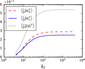
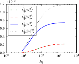
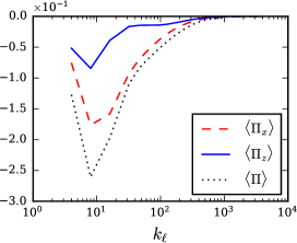
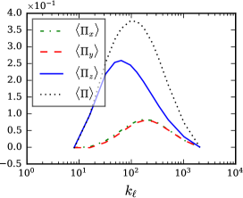
Before delving into details of the budgets in separate directions, we shall first check the coarse-grained kinetic energy in each direction. This is shown as a function of filtering wavenumber in figure 12 for 2D and 3D RT data. In 2D, mean KE is approximately isotropic at all scales, with the horizontal component slightly greater than the vertical at large scales. This may seem counterintuitive since kinetic energy is injected in the vertical direction. In contrast, we see that in 3D, horizontal kinetic energy in and directions are almost equal, but are more than three times smaller than KE in the vertical at large scales. This indicates that in the horizontal plane, 3D-RT turbulent flow is isotropic as expected, but the vertical flow is much stronger than the horizontal at large scales, consistent with results of Cabot & Zhou (2013) based on Fourier spectra in the homogeneous direction. Thus, we have different behaviors for 2D and 3D RT. In 2D-RT, the flow seems to be close to isotropic, while it is highly anisotropic in 3D-RT. Note that in figure 12, derivatives of the plots with respect to give rise to the filtering spectra defined in equation (13). At small scales, the -derivatives of both 2D and 3D filtered KE are small and comparable in all directions. At large scales, the filtering spectrum indicates that the flow is approximately isotropic in 2D (figure 12(a)) and highly anisotropic in 3D (figure 12(b)), where the vertical large-scale flow contains more energy than the horizontal large-scale flow. We will now investigate this difference carefully by analyzing the energy budgets in separate directions.
(a)
(b)
(c)
(d)
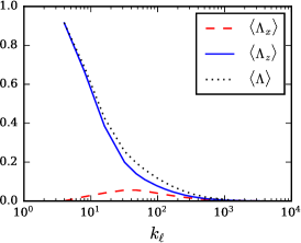
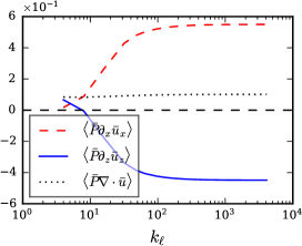
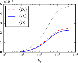
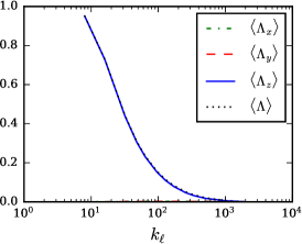
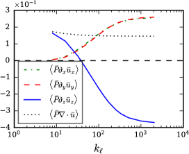
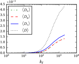
We show in figure 13 mean values of the normalized budget terms in equation (23) for the 2D4096 simulation at time . Budget terms corresponding to the evolution of horizontal KE, vertical KE, and the full KE are shown. In figure 13, is larger in magnitude than , in accordance with the larger magnitude of kinetic energy in the horizontal direction in 2D-RT. The term resides mostly in the vertical component , while is almost zero. This indicates that is mainly responsible for transferring injected energy to vertical scales, and does not redistribute kinetic energy among different directions.
The next term in figure 13 is the (negative) pressure dilatation, which is a cumulative quantity, similar to filtered KE in figure 12, meaning that its contribution at scale is determined by its derivative with respect to filtering wavenumber . That is, its contribution at scale equals . Therefore, as indicated by figure 13, pressure dilatation acts as a source for mean horizontal kinetic energy, since increases with respect to scale, so that its contribution to horizontal KE at scale measured by the derivative is positive. For the mean vertical kinetic energy, the vertical component at the largest scale is positive and acts as a source, but at all subsequent scales its mean value decreases with increasing filtering wavenumber, , indicating it is a sink term at these scales. The combined value in all directions gives rise to a pressure dilatation that is almost constant on average with respect to filtering wavenumber. Therefore, pressure dilatation acts to mix up horizontal and vertical velocities and isotropize the kinetic energy in different directions, similar to the role of pressure-strain in constant-density turbulence (Pope, 2001). Considering dissipation in figure 13, the two components have comparable magnitude, but since there is little kinetic energy residing at small scales due to the fast decay of spectrum and a net upscale cascade by , the magnitude of dissipation in 2D is far smaller than other budget terms.
(a)
(b)
(c)
(d)
The directionally split budget terms for 3D-RT are shown in figure 14. In all four subplots, the and components are equal, indicating isotropy in the horizontal plane. However, anisotropy in the vertical direction is more pronounced than in 2D. in the vertical direction is much larger than the horizontal components, contrary to the 2D case where the horizontal is larger in magnitude. Also in 3D, and peak at smaller scales compared to , indicating a strengthening of the cascade in the horizontal direction at smaller scales, where it becomes more comparable to . Mean is only significant in the vertical direction, with almost zero values in the horizontal directions, similar to 2D. Also, pressure dilatation is the source of kinetic energy input in the horizontal directions, similar to 2D. Dissipation is more isotropic in all directions, consistent with a trend towards isotropy of at these small scales, although the vertical component attains a slightly higher value.
In summary, the directionally split energy budgets in 2D and 3D RT indicates that mean injection and its conduit contribute only to the vertical component of kinetic energy. Horizontal kinetic energy is forced by the horizontal component of pressure dilatation in both 2D and 3D. Dissipation, which is at the smallest scales, is approximately isotropic. However, significant differences between 2D and 3D appear in the fluxes and at inertial scales.
In the earlier discussion of this section, we observed a sharp contrast between 2D and 3D in figure 12, which indicated that the 2D flow is surprisingly isotropic at large-scales, while it is highly anisotropic in 3D due to the expected stronger vertical velocity. The reason can be gleaned from the foregoing results, especially those in figures 13 and 14. The primary difference between the directionally split budgets in 2D and 3D is due to the cascade . In 2D, figure 13(a) shows that is an energy source for mean horizontal large-scale KE, and similarly, is a source for vertical large-scale KE. However, the magnitude of is approximately two to three times greater than , indicating that large-scale KE gains more energy from in the horizontal direction than in the vertical, offsetting anisotropy due to , which energizes the vertical flow. Thus, the inverse cascade acts alongside pressure-dilatation to isotropize the large-scale flow, where most of the kinetic energy resides. In contrast, results from 3D-RT indicate that and are positive, acting as an energy sink for horizontal large-scale KE. Therefore, the large-scale horizontal flow in 3D has only pressure-dilatation as a source of energy, unlike the vertical flow that is being driven by , which ultimately leads to the large anisotropy in 3D-RT.
While the anisotropy analyzed above is due to horizontal and vertical components of the flow, another measure of anisotropy is that of length-scales by using anisotropic filtering kernels as we do in the Supplementary Material, section B.
5 Conclusions
In this work, we have undertaken a thorough analysis of the energy pathways across scales in RT turbulence. We coarse-grained the dynamics using the Favre decomposition to probe nonlinear processes at different scales without resorting to Fourier transforms. In particular, this allowed us to probe scales in the inhomogeneous (vertical) direction, which had not been done before in variable density (non-Boussinesq) RT flows. Our approach does not assume the a priori presence of turbulence and is applicable to general multi-scale flows that may not be considered as turbulent in the traditional sense.
We focused on the role of two flux terms responsible for kinetic energy transfer across scales. One of these, baropycnal work , has been often neglected in LES modeling and lumped with pressure dilatation. Aluie (2011, 2013) had identified as being essential in the transfer of energy across scales in variable density flows such as RT, arising from work done by large-scale pressure gradients on small-scales of density and velocity. Here, we have presented a first analysis of in RT flows and found that it acts as a conduit for potential energy, transferring energy non-locally from the largest scales to smaller scales in the inertial range where the other flux term, , takes over the cascade process.
Unlike , which is inherently due to variations in density, deformation work, , also arises in constant-density flows and may be thought of as representing the process of vortex stretching in 3D, or of vortex mergers in 2D. In 3D-RT, we have shown how takes the energy delivered by at inertial scales and transfers it via a persistent cascade to smaller scales, until it is dissipated at the viscous scales. On the other hand, we have shown how 2D-RT is fundamentally different from 3D, since re-channels the energy back to larger scales, driving a positive feedback loop that is absent in 3D-RT. In this feedback loop, the net upscale cascade leads to an enhanced growth of the mixing layer, which in turn leads to enhanced potential energy release by raising the light fluid and lowering the heavy fluid. The excess PE released results in enhanced baropycnal energy transfer by to smaller scales which is re-channeled back upscale by , closing the feedback loop. Despite higher bulk kinetic energy levels in 2D compared to 3D as a result of this feedback loop, small inertial scales are weaker than in 3D. Our findings also indicate the absence of a net upscale energy transfer in 3D-RT as is often claimed, and that growth of bubbles and spikes at the largest scales is solely due to baropycnal work in 3D.
Our scale analysis demonstrated the presence of an inertial range of scales in RT flows over which kinetic energy fluxes and are not directly influenced by either external inputs at the largest scales or by dissipation at the smallest scales. Our measurement of and over this scale-range revealed that they exhibit a self-similar evolution that is quadratic in time, , similar to the RT mixing layer.
It had been shown by many prior studies that the mixing layer width grows quadratically in time. It had also been often observed that the growth coefficient is significantly larger in 2D than in 3D, despite the precise value of still being an open problem. Our identification of the positive feedback loop in 2D-RT serves to explain this discrepancy as arising from the fundamentally different scale dynamics between 2D and 3D. The possibility of an upscale cascade had been suggested as a possible reason in prior work (Cabot, 2006) but, to our knowledge, never demonstrated by an analysis of energy scale transfer in variable density RT flows before now. We also showed that the net upscale cascade by in 2D tends to isotropize the large-scale flow, in stark contrast to the high level of anisotropy in 3D at large-scales. These differences in the fundamental flow processes highlight the stark disparity between the evolution of 2D-RT and 3D-RT, and pinpoint the potentially misleading physics when employing 2D-RT simulations to model real-world 3D systems.
Acknowledgement
We thank X. Bian, E. Blackman, and D. Livescu for valuable discussions. We also thank the anonymous reviewers for their time and valuable suggestions, which helped improve our manuscript. This research was funded by DOE FES grants DE-SC0014318 and DE-SC0020229. Partial support from NNSA award DE-NA0003856 is acknowledged. HA was also supported by NASA grant 80NSSC18K0772, NSF grant PHY-2020249, DOE grant DE-SC0019329, and NNSA grant DE-NA0003914. Computing time was provided by the National Energy Research Scientific Computing Center (NERSC) under Contract No. DE-AC02-05CH11231, and by an award from the INCITE program, using resources of the Argonne Leadership Computing Facility, which is a DOE Office of Science User Facility supported under Contract DE-AC02-06CH11357. We also acknowledge using data from the JHU Turbulence database (http://turbulence.pha.jhu.edu/).
Declaration of interests
The authors report no conflict of interest.
Appendix A Effects of Interface Mach number
To investigate the influence of interface Mach number (e.g. Wieland et al., 2017) on our conclusions, we performed another 2D-RT simulation using grid points, at a lower Mach number, which we name 2D1024lowM in Table 1. To achieve this, we set the initial pressure at the bottom boundary to be 100, instead of 10 as in simulations 2D4096 and 3D1024, in order to lower the interface Mach number. The interface Mach number, , is based on the ratio between characteristic gravity wave speed , where is the width of the domain, and sound speed at the interface , where is initial temperature at the interface, and is the specific gas constant (Reckinger et al., 2016). The interface Mach number for simulations 2D4096 and 3D1024 in Table 1 is 0.45, while in simulation 2D1024lowM, it is 0.13.
Results from run 2D1024lowM are similar to 2D4096, except for pressure-dilatation as would be expected. Figure 15 shows the mixing width versus time, with growth rate . Figure 16 shows the instantaneous and overall energy budget versus non-dimensional time. The major difference compared to 2D4096 is that pressure-dilatation is greatly suppressed, and the cumulative change of internal energy plays a minor role in 2D1024lowM compared to 2D4096. This is consistent with physical expectations when reducing the compressibility of the RT flow by lowering its Mach number. Figure 17 plots the KE budget terms as a function of scale. All results are consistent with those in figure 7 from run 2D4096, except for the suppressed pressure-dilatation. Finally, figure 18 shows that energy fluxes at low Mach number also exhibit a self-similar behavior.
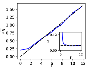
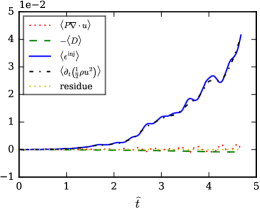
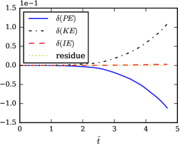
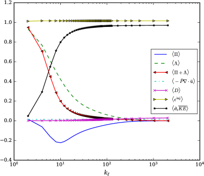
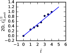
(a)
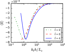
(b)
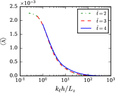
(c)
Appendix B Comparison with 2-species incompressible RT
Throughout the paper we use the single-species two-density model to describe RT flows, but there are other models commonly used in the literature. One notable example is the two-species incompressible model (Sandoval, 1995; Cook & Dimotakis, 2001; Cabot et al., 2004; Livescu & Ristorcelli, 2007, 2008). Here, we compare the energy budgets between the two-species model and our single-species two-density RT model to highlight similarities and differences.
Two-species incompressible RT falls into the category of variable density flows, similar to the compressible model. Governing equations consist of transport equations for each of the two species of mass fraction and , and densities and , respectively. Average density satisfies , where . The dynamics reduces to (Sandoval, 1995; Cook & Dimotakis, 2001; Livescu & Ristorcelli, 2007):
| (24) | ||||
| (25) | ||||
| (26) |
Equation (26) represents the non-zero velocity divergence due to the local change in volume when mixing incompressible fluids of different densities (e.g. Baltzer & Livescu, 2020). is viscous stress tensor as in the compressible equations, and is the binary species diffusivity. The system described by equation (24)-(26) can be obtained (Livescu, 2004) by taking the limit of the compressible equations (1)-(5).
Compared to equations (1)-(5) for compressible dynamics, a key difference is that the two-species model here does not account for internal energy and its coupling to the flow via pressure-dilatation and viscous dissipation. In fact, the primary difference between these two models is a finite (single-species two-density model) versus a zero (two-species model) Mach number (Livescu, 2004, 2020). If we decompose the pressure in equations (1)-(5) into a mean and fluctuation , , and we take the limit , then we approach the limit in the compressible model. Meanwhile, the mean of internal energy equation (4) in this infinite limit reduces to , which is similar to equation (26), except that mass diffusivity in equation (26) is replaced by thermal diffusivity (Livescu, 2013). Thermal diffusivity is defined as , where is thermal conductivity and is the specific heat at constant pressure. Hence, in the limit, the two models are equivalent. Similar to the analysis we have done in section 3.1, by coarse-graining the two-species dynamics, we obtain a large-scale kinetic energy budget of the same form as the filtered KE budget (15).
For a quantitative comparison, we download and analyze the homogeneous buoyancy driven Rayleigh-Taylor data from the Johns Hopkins Turbulence Database (Li et al., 2008; Livescu & Ristorcelli, 2007). The database stores the output of an incompressible two-species RT simulation at a grid resolution. A total of 1015 snapshots are stored densely in time. Unlike our 3D-RT flow presented earlier, this flow is statistically homogeneous in all directions, with a triply periodic domain of equal dimensions, . A spatially uniform pressure gradient is imposed externally and changes with the bulk mixing between species (Livescu & Ristorcelli, 2007). The two species are initialized as random blobs, with a characteristic size of the domain. Flow is driven from rest due to buoyancy, eventually leading to turbulence. However, since the two fluids are miscible, potential energy is ultimately depleted as the fluids mix, leading to turbulence decay. The Atwood number is 0.05, which is close to the Boussinesq limit, but the velocity divergence is nonzero due to the diffusion between the two fluids (Li et al., 2008; Livescu & Ristorcelli, 2007). We download a snapshot at time when the Reynolds number is maximum, and another at when the dissipation rate peaks.
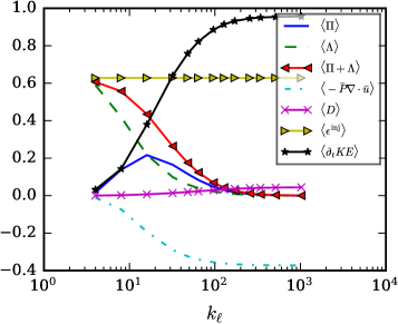
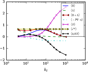
We study the scale dynamics following our earlier analysis in sections 3.2.3-3.2.4. Normalized kinetic energy budget terms are shown in figure 19, with a normalization factor at the corresponding time.
Figure 19(a) shows the result at early time when the RT is still in the developing stage, which is qualitatively similar to our 3D-RT budgets in figure 8. Mean injection is constant in scale, and pressure dilatation saturates at small scales but with a slower convergence rate compared to our results using the compressible Navier-Stokes equations. Fluxes and have a similar scale behavior as in our 3D-RT case. Specifically, both are positive transfering energy to small scales, and peaks at filtering wavenumber . During this developing stage of the flow, the forward cascade via is arrested not by dissipation but by growth of KE at scales smaller than . This can be seen from the plot of , which keeps increasing as a function of until (positive -derivative indicates those scales are experiencing a net gain of KE). Dissipation at this time of the flow (figure 19(a)) is negligible.
At the later time when dissipation is maximum (figure 19(b)), we observe negative values of , indicating decaying turbulence at that time step. Available potential energy is close to being exhausted in this decaying phase of RT, so that the mean injection and become relatively small, while dissipation dominates all other terms. This stage of the homogeneous flow is never reached in our inhomogeneous RT simulations since the effects of walls becomes important at those times. Note in figure 19(b) that unlike the earlier time (figure 19(a)), the forward cascade via operates across a much broader scale range and is arrested by viscous dissipation.
In summary, RT using the two-species incompressible model and RT using the single-species two-density model both belong to the category of variable density flows, and exhibit scale processes in the KE evolution that are similar in many aspects.
References
- Abarzhi (1998) Abarzhi, S I 1998 Stable steady flows in Rayleigh-Taylor instability. Physical Review Letters 81 (2), 337–340.
- Abarzhi (2010) Abarzhi, Snezhana I 2010 Review of theoretical modelling approaches of rayleigh–taylor instabilities and turbulent mixing. Philosophical Transactions of the Royal Society of London A: Mathematical, Physical and Engineering Sciences 368 (1916), 1809–1828.
- Alexakis & Biferale (2018) Alexakis, Alexandros & Biferale, Luca 2018 Cascades and transitions in turbulent flows. Physics Reports 767, 1–101.
- Alon et al. (1995) Alon, U, Hecht, J, Ofer, D & Shvarts, D 1995 Power Laws and Similarity of Rayleigh-Taylor and Richtmyer-Meshkov Mixing Fronts at All Density Ratios. Physical Review Letters 74 (4), 534–537.
- Aluie (2011) Aluie, H. 2011 Compressible Turbulence: The Cascade and its Locality. Phys. Rev. Lett. 106 (17), 174502.
- Aluie (2013) Aluie, Hussein 2013 Scale decomposition in compressible turbulence. Physica D: Nonlinear Phenomena 247 (1), 54–65.
- Aluie & Eyink (2009) Aluie, Hussein & Eyink, Gregory L 2009 Localness of energy cascade in hydrodynamic turbulence. ii. sharp spectral filter. Physics of Fluids 21 (11), 115108.
- Aluie et al. (2018) Aluie, Hussein, Hecht, Matthew & Vallis, Geoffrey K. 2018 Mapping the Energy Cascade in the North Atlantic Ocean: The Coarse-graining Approach. Journal of Physical Oceanography 48, 225–244, arXiv: 1710.07963.
- Aluie et al. (2012) Aluie, Hussein, Li, Shengtai & Li, Hui 2012 Conservative cascade of kinetic energy in compressible turbulence. The Astrophysical Journal Letters 751 (2), L29.
- Anderson et al. (2020) Anderson, KS, Forrest, CJ, Mannion, OM, Marshall, FJ, Shah, RC, Michel, DT, Marozas, JA, Radha, PB, Edgell, DH, Epstein, R & others 2020 Effect of cross-beam energy transfer on target-offset asymmetry in direct-drive inertial confinement fusion implosions. Physics of Plasmas 27 (11), 112713.
- Baltzer & Livescu (2020) Baltzer, Jon R & Livescu, Daniel 2020 Variable-density effects in incompressible non-buoyant shear-driven turbulent mixing layers. Journal of Fluid Mechanics 900.
- Banerjee et al. (2010) Banerjee, Arindam, Kraft, Wayne N & Andrews, Malcolm J 2010 Detailed measurements of a statistically steady rayleigh-taylor mixing layer from small to high atwood numbers. JFM 659, 127–190.
- Bestehorn (2020) Bestehorn, Michael 2020 Rayleigh–taylor and kelvin–helmholtz instability studied in the frame of a dimension-reduced model. Philosophical Transactions of the Royal Society A 378 (2174), 20190508.
- Betti & Hurricane (2016) Betti, R & Hurricane, OA 2016 Inertial-confinement fusion with lasers. Nature Physics 12 (5), 435.
- Bian et al. (2020) Bian, Xin, Aluie, Hussein, Zhao, Dongxiao, Zhang, Huasen & Livescu, Daniel 2020 Revisiting the late-time growth of single-mode rayleigh–taylor instability and the role of vorticity. Physica D: Nonlinear Phenomena 403, 132250.
- Birkhoff (1955) Birkhoff, Garrett 1955 Taylor instability and laminar mixing. Tech. Rep.. Los Alamos National Laboratory, report LA-1862.
- Bodony & Lele (2005) Bodony, Daniel J & Lele, Sanjiva K 2005 On using large-eddy simulation for the prediction of noise from cold and heated turbulent jets. Physics of Fluids 17 (8), 085103.
- Boffetta et al. (2012) Boffetta, Guido, De Lillo, Filippo, Mazzino, Andrea & Musacchio, Stefano 2012 Bolgiano scale in confined rayleigh–taylor turbulence. Journal of Fluid Mechanics 690, 426–440.
- Boffetta & Ecke (2012) Boffetta, Guido & Ecke, Robert E 2012 Two-dimensional turbulence. Annual Review of Fluid Mechanics 44, 427–451.
- Boffetta & Mazzino (2017) Boffetta, Guido & Mazzino, Andrea 2017 Incompressible rayleigh–taylor turbulence. Annual Review of Fluid Mechanics 49, 119–143.
- Boffetta et al. (2009) Boffetta, G, Mazzino, A, Musacchio, S & Vozella, L 2009 Kolmogorov scaling and intermittency in rayleigh-taylor turbulence. Physical Review E 79 (6), 065301.
- Brady & Livescu (2019) Brady, Peter T & Livescu, Daniel 2019 High-order, stable, and conservative boundary schemes for central and compact finite differences. Computers & Fluids 183, 84–101.
- Burton (2011) Burton, Gregory C 2011 Study of ultrahigh Atwood-number Rayleigh–Taylor mixing dynamics using the nonlinear large-eddy simulation method. Physics of Fluids 23 (4), 045106.
- Cabot (2006) Cabot, W 2006 Comparison of two-and three-dimensional simulations of miscible rayleigh-taylor instability. Physics of Fluids 18 (4), 045101.
- Cabot & Zhou (2013) Cabot, W & Zhou, Ye 2013 Statistical measurements of scaling and anisotropy of turbulent flows induced by rayleigh-taylor instability. Physics of Fluids 25 (1), 015107.
- Cabot & Cook (2006) Cabot, William H & Cook, Andrew W 2006 Reynolds number effects on rayleigh–taylor instability with possible implications for type ia supernovae. Nature Physics 2 (8), 562–568.
- Cabot et al. (2004) Cabot, William H, Schilling, Oleg & Zhou, Ye 2004 Influence of subgrid scales on resolvable turbulence and mixing in rayleigh–taylor flow. Physics of Fluids 16 (3), 495–508.
- Carpenter et al. (2020) Carpenter, KR, Mancini, RC, Harding, EC, Harvey-Thompson, AJ, Geissel, M, Weis, MR, Hansen, SB, Peterson, KJ & Rochau, GA 2020 Temperature distributions and gradients in laser-heated plasmas relevant to magnetized liner inertial fusion. Physical Review E 102 (2), 023209.
- Chassaing (1985) Chassaing, P 1985 An alternative formulation of the equations of turbulent motion for a fluid of variable density. Journal de Mecanique Theorique et Appliquee 4, 375–389.
- Chen et al. (2020) Chen, Ke-Jung, Woosley, SE & Whalen, Daniel J 2020 Gas dynamics of the nickel-56 decay heating in pair-instability supernovae. The Astrophysical Journal 897 (2), 152.
- Cheng et al. (2002) Cheng, Baolian, Glimm, J. & Sharp, D H 2002 A three-dimensional renormalization group bubble merger model for Rayleigh–Taylor mixing. Chaos: An Interdisciplinary Journal of Nonlinear Science 12 (2), 267–274.
- Chertkov (2003) Chertkov, Michael 2003 Phenomenology of rayleigh-taylor turbulence. Physical review letters 91 (11), 115001.
- Clark et al. (2016) Clark, D S, Weber, C R, Milovich, J L, Salmonson, J D, Kritcher, A L, Haan, S W, Hammel, B A, Hinkel, D E, Hurricane, O A, Jones, O S, Marinak, M M, Patel, P K, Robey, H F, Sepke, S M & Edwards, M J 2016 Three-dimensional simulations of low foot and high foot implosion experiments on the National Ignition Facility. Physics of Plasmas 23 (5), 056302.
- Cook & Dimotakis (2001) Cook, Andrew W & Dimotakis, Paul E 2001 Transition stages of rayleigh–taylor instability between miscible fluids. Journal of Fluid Mechanics 443, 69–99.
- Cook & Zhou (2002) Cook, Andrew W & Zhou, Ye 2002 Energy transfer in Rayleigh-Taylor instability. Physical Review E 66 (2), 192.
- Dimonte (2004) Dimonte, Guy 2004 Dependence of turbulent rayleigh-taylor instability on initial perturbations. Physical Review E 69 (5), 056305.
- Dimonte et al. (2005) Dimonte, Guy, Ramaprabhu, P, Youngs, DL, Andrews, MJ & Rosner, R 2005 Recent advances in the turbulent rayleigh–taylor instability a. Physics of plasmas 12 (5), 056301.
- Dimonte et al. (2004) Dimonte, Guy, Youngs, DL, Dimits, A, Weber, S, Marinak, M, Wunsch, S, Garasi, C, Robinson, A, Andrews, MJ, Ramaprabhu, P & others 2004 A comparative study of the turbulent rayleigh–taylor instability using high-resolution three-dimensional numerical simulations: the alpha-group collaboration. Physics of Fluids 16 (5), 1668–1693.
- Douglas et al. (1998) Douglas, M R, Deeney, C & Roderick, N F 1998 Computational investigation of single mode vs multimode Rayleigh-Taylor seeding in Z-pinch implosions. Physics of Plasmas 5 (1), 4183–4198.
- Eyink (1995) Eyink, Gregory L 1995 Exact Results on Scaling Exponents in the 2D Enstrophy Cascade. Physical Review Letters 74 (1), 3800–3803.
- Eyink (2005) Eyink, Gregory L 2005 Locality of turbulent cascades. Physica D: Nonlinear Phenomena 207 (1), 91–116.
- Eyink (2006) Eyink, Gregory L 2006 Multi-scale gradient expansion of the turbulent stress tensor. Journal of Fluid Mechanics 549, 159–190.
- Eyink & Aluie (2009) Eyink, Gregory L & Aluie, Hussein 2009 Localness of energy cascade in hydrodynamic turbulence. i. smooth coarse graining. Physics of Fluids 21 (11), 115107.
- Eyink & Drivas (2018) Eyink, Gregory L & Drivas, Theodore D 2018 Cascades and dissipative anomalies in compressible fluid turbulence. Physical Review X 8 (1), 011022.
- Fang & Ouellette (2016) Fang, Lei & Ouellette, Nicholas T 2016 Advection and the Efficiency of Spectral Energy Transfer in Two-Dimensional Turbulence. Physical Review Letters 117 (10), 104501.
- Favre et al. (1958) Favre, AJ, Gaviglio, JJ & Dumas, RJ 1958 Further space-time correlations of velocity in a turbulent boundary layer. Journal of Fluid Mechanics 3 (4), 344–356.
- Gerashchenko & Livescu (2016) Gerashchenko, S. & Livescu, D. 2016 Viscous effects on the Rayleigh-Taylor instability with background temperature gradient. Physics of Plasmas 23 (7), 072121.
- Germano (1992) Germano, M 1992 Turbulence: the filtering approach. Journal of Fluid Mechanics 238, 325–336.
- Glimm & Li (1988) Glimm, James & Li, XL 1988 Validation of the sharp–wheeler bubble merger model from experimental and computational data. The Physics of fluids 31 (8), 2077–2085.
- Glimm et al. (2013) Glimm, J., Sharp, D H, Kaman, T. & Lim, H. 2013 New directions for Rayleigh-Taylor mixing. Philosophical Transactions of the Royal Society A: Mathematical 371, 20120183–20120183.
- Goncharov (2002) Goncharov, VN 2002 Analytical model of nonlinear, single-mode, classical rayleigh-taylor instability at arbitrary atwood numbers. Physical review letters 88 (13), 134502.
- Hillebrandt & Niemeyer (2000) Hillebrandt, Wolfgang & Niemeyer, Jens C 2000 Type ia supernova explosion models. Annual Review of Astronomy and Astrophysics 38 (1), 191–230.
- Hopkins et al. (2018) Hopkins, L Berzak, LePape, S, Divol, L, Pak, A, Dewald, E, Ho, DD, Meezan, N, Bhandarkar, S, Benedetti, LR, Bunn, T & others 2018 Toward a burning plasma state using diamond ablator inertially confined fusion (icf) implosions on the national ignition facility (nif). Plasma Physics and Controlled Fusion 61 (1), 014023.
- Horne & Lawrie (2020) Horne, J T & Lawrie, A G W 2020 Aspect-ratio-constrained Rayleigh-Taylor instability. Physica D: Nonlinear Phenomena 406, 132442.
- Joggerst et al. (2010) Joggerst, C C, Almgren, A & Woosley, S E 2010 Three-Dimensional Simulations Of Rayleigh-Taylor Mixing In Core-Collapse Supernovae. Astrophysical Journal 723 (1), 353–363.
- John (2012) John, Volker 2012 Large eddy simulation of turbulent incompressible flows: analytical and numerical results for a class of LES models, , vol. 34. Springer Science & Business Media.
- Just et al. (2018) Just, Oliver, Bollig, Robert, Janka, H-Th, Obergaulinger, Martin, Glas, Robert & Nagataki, Shigehiro 2018 Core-collapse supernova simulations in one and two dimensions: comparison of codes and approximations. Monthly Notices of the Royal Astronomical Society 481 (4), 4786–4814.
- Karimi & Girimaji (2017) Karimi, Mona & Girimaji, Sharath S 2017 Influence of orientation on the evolution of small perturbations in compressible shear layers with inflection points. Physical Review E 95 (3).
- Kida & Orszag (1990) Kida, Shigeo & Orszag, Steven A 1990 Energy and spectral dynamics in forced compressible turbulence. Journal of Scientific Computing 5 (2), 85–125.
- Kolmogorov (1941) Kolmogorov, Andrey Nikolaevich 1941 The local structure of turbulence in incompressible viscous fluid for very large reynolds numbers. Cr Acad. Sci. URSS 30, 301–305.
- Kotake et al. (2018) Kotake, Kei, Takiwaki, Tomoya, Fischer, Tobias, Nakamura, Ko & Martínez-Pinedo, Gabriel 2018 Impact of Neutrino Opacities on Core-collapse Supernova Simulations. The Astrophysical Journal 853 (2), 170.
- Kraichnan (1967) Kraichnan, Robert H 1967 Inertial ranges in two-dimensional turbulence. The Physics of Fluids 10 (7), 1417–1423.
- Kritsuk et al. (2013) Kritsuk, Alexei G, Wagner, Rick & Norman, Michael L 2013 Energy cascade and scaling in supersonic isothermal turbulence. Journal of Fluid Mechanics 729.
- Kull (1991) Kull, Hans-Jörg 1991 Theory of the rayleigh-taylor instability. Physics Reports 206 (5), 197–325.
- Lawrie & Dalziel (2011) Lawrie, Andrew GW & Dalziel, Stuart B 2011 Rayleigh-taylor mixing in an otherwise stable stratification. Journal of fluid mechanics 688, 507.
- Layzer (1955) Layzer, David 1955 On the instability of superposed fluids in a gravitational field. The astrophysical journal 122, 1.
- Lees & Aluie (2019) Lees, Aarne & Aluie, Hussein 2019 Baropycnal work: A mechanism for energy transfer across scales. Fluids 4 (2), 92.
- Lele (1992) Lele, Sanjiva K 1992 Compact finite difference schemes with spectral-like resolution. Journal of computational physics 103 (1), 16–42.
- Leonard (1975) Leonard, A 1975 Energy cascade in large-eddy simulations of turbulent fluid flows. Advances in geophysics 18, 237–248.
- Li et al. (2008) Li, Yi, Perlman, Eric, Wan, Minping, Yang, Yunke, Meneveau, Charles, Burns, Randal, Chen, Shiyi, Szalay, Alexander & Eyink, Gregory 2008 A public turbulence database cluster and applications to study lagrangian evolution of velocity increments in turbulence. Journal of Turbulence (9), N31.
- Livescu (2004) Livescu, Daniel 2004 Compressibility effects on the rayleigh–taylor instability growth between immiscible fluids. Physics of Fluids 16 (1), 118–127.
- Livescu (2013) Livescu, D 2013 Numerical simulations of two-fluid turbulent mixing at large density ratios and applications to the Rayleigh-Taylor instability. Philosophical Transactions of the Royal Society a-Mathematical Physical and Engineering Sciences 371 (2003).
- Livescu (2020) Livescu, Daniel 2020 Turbulence with large thermal and compositional density variations. Annual Review of Fluid Mechanics 52, 309–341.
- Livescu & Ristorcelli (2007) Livescu, Daniel & Ristorcelli, JR 2007 Buoyancy-driven variable-density turbulence. Journal of Fluid Mechanics 591, 43–71.
- Livescu & Ristorcelli (2008) Livescu, Daniel & Ristorcelli, JR 2008 Variable-density mixing in buoyancy-driven turbulence. Journal of Fluid Mechanics 605, 145–180.
- Livescu et al. (2009) Livescu, Daniel, Ristorcelli, JR, Gore, RA, Dean, SH, Cabot, WH & Cook, AW 2009 High-reynolds number rayleigh–taylor turbulence. Journal of Turbulence (10), N13.
- Livescu et al. (2010) Livescu, D, Ristorcelli, JR, Petersen, MR & Gore, RA 2010 New phenomena in variable-density rayleigh–taylor turbulence. Physica Scripta 2010 (T142), 014015.
- Meaney et al. (2020) Meaney, Kevin Daniel, Kim, Y, Geppert-Kleinrath, Hermann, Herrmann, Hans W, Berzak Hopkins, L, Hoffman, Nelson M, Cerjan, C, Landen, Otto L, Baker, K, Carrera, J & others 2020 Carbon ablator areal density at fusion burn: Observations and trends at the national ignition facility. Physics of Plasmas 27 (5), 052702.
- Meneveau (1994) Meneveau, Charles 1994 Statistics of turbulence subgrid-scale stresses: Necessary conditions and experimental tests. Physics of Fluids 6 (2), 815–833.
- Meneveau & Katz (2000) Meneveau, C. & Katz, J. 2000 Scale-Invariance and Turbulence Models for Large-Eddy Simulation. Ann. Rev. Fluid Mech. 32, 1–32.
- Ofer et al. (1996) Ofer, D, Alon, U, Shvarts, D, Mccrory, R L & Verdon, C P 1996 Modal model for the nonlinear multimode Rayleigh-Taylor instability. Physics of Plasmas 3 (8), 3073–3090.
- Olson & Jacobs (2009) Olson, DH & Jacobs, JW 2009 Experimental study of rayleigh–taylor instability with a complex initial perturbation. Physics of Fluids 21 (3), 034103.
- Oron et al. (2001) Oron, D, Arazi, L, Kartoon, D, Rikanati, A, Alon, U & Shvarts, D 2001 Dimensionality dependence of the Rayleigh–Taylor and Richtmyer–Meshkov instability late-time scaling laws. Physics of Plasmas 8 (6), 2883–2889.
- Patterson & Orszag (1971) Patterson, GS & Orszag, Steven A 1971 Spectral calculations of isotropic turbulence: Efficient removal of aliasing interactions. The Physics of Fluids 14 (11), 2538–2541.
- Piomelli et al. (1991) Piomelli, Ugo, Cabot, William H, Moin, Parviz & Lee, Sangsan 1991 Subgrid-scale backscatter in turbulent and transitional flows. Physics of Fluids A: Fluid Dynamics 3 (7), 1766–1771.
- Pope (2001) Pope, Stephen B 2001 Turbulent flows. IOP Publishing.
- Porth et al. (2014) Porth, Oliver, Komissarov, Serguei S. & Keppens, Rony 2014 Rayleigh–Taylor instability in magnetohydrodynamic simulations of the Crab nebula. Monthly Notices of the Royal Astronomical Society 443 (1), 547–558.
- Ramaprabhu et al. (2005) Ramaprabhu, P, Dimonte, Guy & Andrews, MJ 2005 A numerical study of the influence of initial perturbations on the turbulent rayleigh–taylor instability. Journal of Fluid Mechanics 536, 285–319.
- Ramaprabhu et al. (2012) Ramaprabhu, P, Dimonte, Guy, Woodward, P, Fryer, C, Rockefeller, G, Muthuraman, K, Lin, P-H & Jayaraj, J 2012 The late-time dynamics of the single-mode rayleigh-taylor instability. Physics of Fluids 24 (7), 074107.
- Rayleigh (1883) Rayleigh 1883 Investigation of the character of the equilibrium of an incompressible heavy fluid of variable density. Proceedings of the London Mathematical Society s1-14 (1), 170–177.
- Reckinger et al. (2016) Reckinger, Scott J, Livescu, Daniel & Vasilyev, Oleg V 2016 Comprehensive numerical methodology for direct numerical simulations of compressible rayleigh–taylor instability. Journal of Computational Physics 313, 181–208.
- Ristorcelli & Clark (2004) Ristorcelli, JR & Clark, TT 2004 Rayleigh–taylor turbulence: self-similar analysis and direct numerical simulations. Journal of Fluid Mechanics 507, 213–253.
- Rivera et al. (2014) Rivera, MK, Aluie, Hussein & Ecke, RE 2014 The direct enstrophy cascade of two-dimensional soap film flows. Physics of Fluids 26 (5), 055105.
- Sadek & Aluie (2018) Sadek, Mahmoud & Aluie, Hussein 2018 Extracting the spectrum of a flow by spatial filtering. Physical Review Fluids 3 (12), 124610.
- Saenz et al. (2021) Saenz, JA, Aslangil, D & Livescu, D 2021 Filtering, averaging, and scale dependency in homogeneous variable density turbulence. Physics of Fluids 33 (2), 025115.
- Sandoval (1995) Sandoval, Donald L. 1995 The dynamics of variable-density turbulence. PhD thesis, University of Washington.
- Schilling & Mueschke (2010) Schilling, Oleg & Mueschke, Nicholas J 2010 Analysis of turbulent transport and mixing in transitional rayleigh–taylor unstable flow using direct numerical simulation data. Physics of Fluids 22 (10), 105102.
- Sharp (1984) Sharp, David H 1984 An overview of rayleigh-taylor instability. Physica D: Nonlinear Phenomena 12 (1-3), 3IN111–10IN1018.
- Shvarts et al. (1995) Shvarts, D, Alon, U, Ofer, D, Mccrory, R L & Verdon, C P 1995 Nonlinear evolution of multimode Rayleigh-Taylor instability in two and three dimensions. Physics of Plasmas 2 (6), 2465–2472.
- Taylor (1950) Taylor, Geoffrey 1950 The instability of liquid surfaces when accelerated in a direction perpendicular to their planes. i. Proceedings of the Royal Society of London. Series A. Mathematical and Physical Sciences 201 (1065), 192–196.
- Wang et al. (2018) Wang, Jianchun, Wan, Minping, Chen, Song & Chen, Shiyi 2018 Kinetic energy transfer in compressible isotropic turbulence. Journal of Fluid Mechanics 841, 581–613.
- Wang et al. (2013) Wang, Jianchun, Yang, Yantao, Shi, Yipeng, Xiao, Zuoli, He, XT & Chen, Shiyi 2013 Cascade of kinetic energy in three-dimensional compressible turbulence. Physical review letters 110 (21), 214505.
- Weber et al. (2020) Weber, CR, Clark, DS, Pak, A, Alfonso, N, Bachmann, B, Berzak Hopkins, LF, Bunn, T, Crippen, J, Divol, L, Dittrich, T & others 2020 Mixing in icf implosions on the national ignition facility caused by the fill-tube. Physics of Plasmas 27 (3), 032703.
- Weber et al. (2014) Weber, C R, Clark, D S, Cook, A W, Busby, L E & Robey, H F 2014 Inhibition of turbulence in inertial-confinement-fusion hot spots by viscous dissipation. Physical Review E 89 (5), 362.
- Wei & Livescu (2012) Wei, Tie & Livescu, Daniel 2012 Late-time quadratic growth in single-mode rayleigh-taylor instability. Physical Review E 86 (4), 046405.
- Wei et al. (2017) Wei, Yikun, Dou, Hua-Shu, Qian, Yuehong & Wang, Zhengdao 2017 A novel two-dimensional coupled lattice boltzmann model for incompressible flow in application of turbulence rayleigh–taylor instability. Computers & Fluids 156, 97–102.
- Wieland et al. (2017) Wieland, Scott, Reckinger, Scott, Hamlington, Peter E & Livescu, Daniel 2017 Effects of background stratification on the compressible rayleigh taylor instability. In 47th AIAA Fluid Dynamics Conference, p. 3974.
- Wieland et al. (2019) Wieland, Scott A, Hamlington, Peter E, Reckinger, Scott J & Livescu, Daniel 2019 Effects of isothermal stratification strength on vorticity dynamics for single-mode compressible Rayleigh-Taylor instability. Physical Review Fluids 4 (9), 093905.
- Youngs (1991) Youngs, David L 1991 Three-dimensional numerical simulation of turbulent mixing by rayleigh–taylor instability. Physics of Fluids A: Fluid Dynamics 3 (5), 1312–1320.
- Youngs (1994) Youngs, David L 1994 Numerical simulation of mixing by rayleigh–taylor and richtmyer–meshkov instabilities. Laser and particle beams 12 (4), 725–750.
- Zhang et al. (2018a) Zhang, H, Betti, R, Gopalaswamy, V, Yan, R & Aluie, H 2018a Nonlinear excitation of the ablative rayleigh-taylor instability for all wave numbers. Physical Review E 97 (1), 011203.
- Zhang et al. (2018b) Zhang, Huasen, Betti, Riccardo, Yan, R, Zhao, D, Shvarts, D & Aluie, H 2018b Self-similar multimode bubble-front evolution of the ablative rayleigh-taylor instability in two and three dimensions. Physical review letters 121 (18), 185002.
- Zhang et al. (2018c) Zhang, J, Wang, LF, Ye, WH, Wu, JF, Guo, HY, Ding, YK, Zhang, WY & He, XT 2018c Weakly nonlinear multi-mode rayleigh-taylor instability in two-dimensional spherical geometry. Physics of Plasmas 25 (8), 082713.
- Zhao & Aluie (2018) Zhao, Dongxiao & Aluie, Hussein 2018 Inviscid criterion for decomposing scales. Physical Review Fluids 3 (5), 054603.
- Zhao et al. (in preparation) Zhao, Dongxiao, Betti, Riccardo & Aluie, Hussein in preparation Energy pathways in single-mode rayleigh-taylor flows .
- Zhou et al. (2016) Zhou, Quan, Huang, Yong-Xiang, Lu, Zhi-Ming, Liu, Yu-Lu & Ni, Rui 2016 Scale-to-scale energy and enstrophy transport in two-dimensional rayleigh–taylor turbulence. Journal of Fluid Mechanics 786, 294–308.
- Zhou (2001) Zhou, Ye 2001 A scaling analysis of turbulent flows driven by rayleigh–taylor and richtmyer–meshkov instabilities. Physics of Fluids 13 (2), 538–543.
- Zhou (2017a) Zhou, Ye 2017a Rayleigh–taylor and richtmyer–meshkov instability induced flow, turbulence, and mixing. i. Physics Reports 720, 1–136.
- Zhou (2017b) Zhou, Ye 2017b Rayleigh–taylor and richtmyer–meshkov instability induced flow, turbulence, and mixing. ii. Physics Reports 723, 1–160.
- Zhou (2021) Zhou, Ye 2021 Turbulence theories and statistical closure approaches. Physics Reports .
- Zhou & Cabot (2019) Zhou, Ye & Cabot, William H 2019 Time-dependent study of anisotropy in rayleigh-taylor instability induced turbulent flows with a variety of density ratios. Physics of Fluids 31 (8), 084106.
- Zhou et al. (2003) Zhou, Ye, Remington, BA, Robey, HF, Cook, AW, Glendinning, SG, Dimits, A, Buckingham, AC, Zimmerman, GB, Burke, EW, Peyser, TA & others 2003 Progress in understanding turbulent mixing induced by rayleigh–taylor and richtmyer–meshkov instabilities. Physics of Plasmas 10 (5), 1883–1896.
Supplementary Information for “Scale interactions and anisotropy in Rayleigh-Taylor turbulence” by Dongxiao Zhao, Riccardo Betti, and Hussein Aluie
A Efficiency of the fluxes
We have observed (figures 7-8 in the main text) that baropycnal work dominates at the largest scales. It acts as a conduit for mean injection from potential energy by transferring energy from the largest scales to smaller scales in the inertial range where deformation work takes over and dominates the cascade process.
Since this work is the first to investigate as a function of scale , a basic question that arises is whether its decay at small is due to a decay in its magnitude or due to a mis-alignment of and . We shall answer the question in this subsection. We first reiterate the flux expressions in equation (19) in the main text for convenience:
where is the Favre filtered velocity strain tensor. Following (\citeSuppLiao14,FangOuellette16,Ouellette18), we define the cascade efficiency and to be
| (S-1) | ||||
which resembles the cosine of the angle between two vectors. These definitions in equation (S-1) follow that in \citeSuppOuellette18 who studied the cascade efficiency in constant-density turbulence. By the Cauchy-Schwartz inequality, .
Similarly, the magnitudes of these two fluxes, denoted by and , are defined by the denominator in the flux efficiency equation (S-1):
| (S-2) | ||||
and can be regarded as the product of tensor magnitudes. The actual and terms are proportional to the product of efficiency and magnitude
with a proportionality factor involving density.
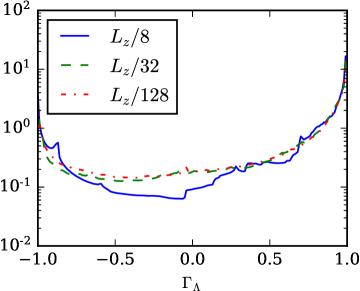
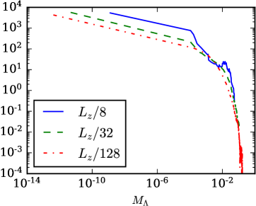
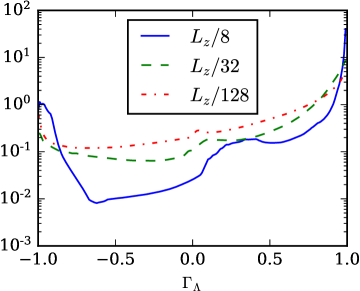
(a)
(b)
(c)
(d)
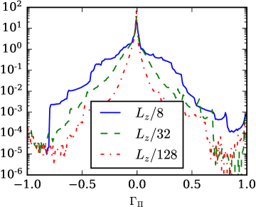
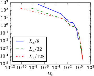
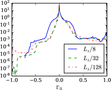
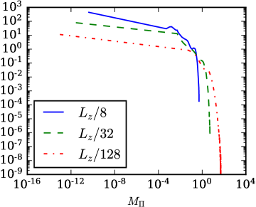
The cascade efficiency and magnitude of in 2D and 3D are shown in figure S1. Magnitude in both 2D and 3D decreases at smaller scales as appears in figures 1(b) and 1(d). In fact, figure S2(b) shows that seems to scale . This decay can be understood from basic scaling estimates for the magnitude of , following (\citeSuppEyink_notes,Eyink05,Aluie11c). We first observe that in our flows, both 2D and 3D, the pressure field is mostly smooth as evidenced by the scaling of its filtering spectrum in figure S2(a), decaying at least as fast333As \citeSuppSadek18 elaborate, the filtering spectrum for a field with actual scaling that is steeper than will appear as when using 1st-order filtering kernels such as a Gaussian. as , where is filtering wavenumber (inverse of scale). Therefore, the pressure gradient is dominated by the largest scale ,
and is (to leading order) independent of , where an increment is defined as usual, . Here, is a characteristic large scale of RT, comparable to the domain size. On the other hand, subscale mass flux scales as (\citeSuppAluie11c):
where , and from figure 5, the two scaling exponents , yielding . This explains decay of as a function of filtering wavenumber in both 2D and 3D-RT. The decay is faster in the dissipation range since fluctuations giving rise to decay faster at those scales.
An important conclusion from the scaling of the pressure spectrum in figure S2(a) is that energy transfer by is (infrared) non-local in scale due to dominance of the largest scale in the pressure gradient (\citeSuppEyink05,EyinkAluie09,Aluie11c). This is similar to energy transfer in the Batchelor range of magnetohydrodynamic turbulence at high magnetic Prandtl numbers (\citeSuppbatchelor1959small,AluieEyink10), where energy is transferred nonlocally from the flow at viscous scales to the magnetic field at much smaller scales due to smoothness of the velocity at those small viscous scales. We note, however, that such non-local transfer by is mostly likely a hallmark of RT turbulence, where is dominated by the largest scales in the system, and may not hold in general variable density turbulence in which the pressure field is not smooth (\citeSuppAluie11c).
While the magnitude decays at smaller scales both in 2D-RT and 3D-RT, efficiency seems to have a much weaker decay at small scales. Figure S1(a) shows that in 2D-RT is almost independent of scale, which is reinforced by scaling plots in figure S2(c). In 3D-RT, figure S2(c) shows a very shallow scaling, with .
To explain the decay of at small scales we observed in 2D-RT (figure 7 in the main text) and in 3D-RT (figure 8 in the main text), we assume that the efficiency and magnitude of are statistically independent, (within the factor ). When this is combined the above observations on the scaling of each of and , we are able to explain the decay of , which figure S2(d) shows to be in 2D and in 3D. Therefore, we can conclude from the foregoing discussion that the decay in at smaller is primarily due to a decay in its magnitude rather than due to a mis-alignment of and .
Unlike , which decays monotonically in the inertial range, deformation work peaks in the inertial range as it takes over the energy transfer process. PDFs of the efficiency of (figures S3(a),(c)) indicate a profound difference from . Whereas the PDFs of in figures S2(a) and (c) peak around the maximum possible values, -1 and 1, has a highest probability around zero. This is consistent with the investigation by \citeSuppOuellette18, who concluded that is inefficient at transferring energy in constant-density homogeneous turbulence (see also \citeSuppFangOuellette16). Thus, the flux, which transfers energy due to subscale stress acting against a larger-scale strain, is less efficient than , which operates by the barotropic and baroclinic generation of vorticity and strain (\citeSuppAarne19,ZhaoAluie20).
B and with anisotropic filters
In section 4 of the main text, we analyzed how the fluxes can lead to anisotropic motion in different directions by directional splitting of the kinetic energy budget, which we coarse-grained with isotropic kernels. In this section, we shall quantify the anisotropy of length-scales energized by and , through coarse-graining with anisotropic kernels. We use the following ‘horizontal kernel’ and ‘vertical kernel’:
which perform the filtering operation in only one direction. These filters only capture the spectral information in the corresponding direction and ignore variations in the other directions. We denote the fluxes calculated by these anisotropic kernels using notation such as or . Note that unlike the ‘directionally split’ analysis presented earlier, here the sum of anisotropically filtered fluxes does not equal the full flux, i.e., .
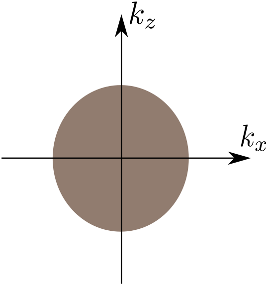
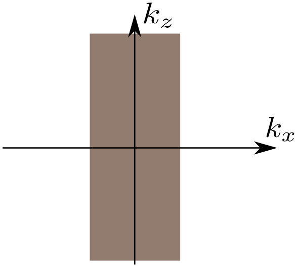
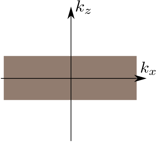
The essence of isotropic and anisotropic filtering is illustrated in figure S4 in -space, where filtering wavenumbers are only a proxy for length-scales, but can be conceptually associated with Fourier wavenumbers commonly used in the community. Here, is any characteristic large-scale to be used only as a common reference in all directions to define filtering wavenumbers. Figure S4 depicts a two-dimensional wavenumber space, with horizontal and vertical filtering wavenumbers corresponding to scales in the x-direction and z-direction, respectively. Isotropic filtering with kernel retains scales within the shaded sphere in -space (figure 4(a)), satisfying . On the other hand, anisotropic filtering with kernel , for example, retains scales within the shaded slab in -space (figure 4(b)), satisfying but does not allow us to probe scales in the z-direction since it does not partition those scales. The analysis generalizes to 3D in a straightforward way.
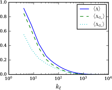
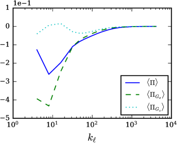
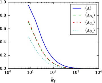
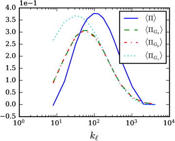
Mean anisotropic fluxes of the 2D4096 and 3D1024 data, at time , are shown in figure S5. For baropycnal work , both the 2D and 3D results shown in figures 5(a) and 5(c) indicate that is larger than . This implies that most of the potential energy is being transferred to horizontal scales, although nonzero transfer is also creating flow variation in the vertical direction. The tendency of baropycnal transfer in energizing small-scales along the x-direction is consistent with our understanding of RT instability during the linear stage when potential energy feeds perturbations that vary in the horizontal direction. Figures 5(a),5(c) indicate that baropycnal transfer from potential energy at later times, when the flow becomes nonlinear, also participates in the creation of vertical scales. This is consistent with the association of baropycnal work with vorticity and strain creation (\citeSuppAarne19), which necessarily involve small-scales in the vertical direction. Nevertheless, horizontal scale creation still dominates at late times, with at all scales. Note that in 3D, we have in figure 5(c), indicating that horizontal scales are being energized isotropically by , as expected.
Probing anisotropy of deformation work , we can observe significant differences between the 2D case, shown in figure 5(b), and the 3D case, shown in figure 5(d). In 2D, the mean value of calculated from isotropic kernel is negative, and so is the anisotropic . On the other hand, mean attains positive values over a certain range of scales. Since is primarily determined by the velocity fields, we shall focus on the characteristics of velocity fields in RT evolution. The positive measures energy transfer across vertical scales, which goes into sustaining the ‘mixing fronts,’ which are the two envelopes enclosing the mixing layer in RT turbulence. We verified this from visualizations of (not shown here). This is similar to the downscale energy transfer that forms and sustains the shock front in a 1D Burgers flow. In our RT flow, the velocity profile along the z-axis comprises of a vertical flow inside the mixing layer pushing against a more quiescent fluid outside. Such fronts necessarily involve small vertical scales that need to be constantly replenished by , otherwise the front would broaden. We find that inside the mixing layer (not shown), away from the fronts, , transferring net energy upscale as in a homogeneous 2D flow. However, the contribution from the front regions is stronger such that overall . Despite being positive, is much smaller than the net upscale transfer in the horizontal direction measured by in figure 5(b), which dominates the cross-scale transfer when we treat all directions equally by using isotropic kernels to measure in figure 5(b). In the 3D-RT flow, we see in figure 5(d) that , , and are all positive, transferring energy downscale. We find that peaks at slightly larger scales and again plays a role in the formation of the mixing fronts as in 2D, while , indicating isotropic downscale transfer in the horizontal scales.
We also note that at all scales, indicating that the ‘mixing front’ propagation plays an important role in the downscale kinetic energy transfer. This aspect of energy transfer was missing in previous studies relying on FFTs in the horizontal while neglecting vertical scales.
C Filtering Spectra of Kinetic Energy
Here, we compare the ‘filtering’ spectra using three different scale-decompositions to define kinetic energy, following \citeSuppZhao18. In variable density flows, scale decomposition is not as straightforward as in constant density flows. One possible decomposition is to define large-scale kinetic energy as , which has been used in many studies (e.g. \citeSuppchassaing1985alternative,BodonyLele05,Burton11,KarimiGirimaji17). Another possibility is to define large-scale kinetic energy as , which has also been used extensively in compressible turbulence studies (e.g. \citeSuppkida1990energy,CookZhou02,Wang13,Greteetal17). A third is based on the Favre decomposition (\citeSuppHesselberg26,Favre58a), which we adopt in this work, and uses as the definition for large-scale kinetic energy, where .
Zhao18 demonstrated numerically that these three different quantities, all of which have units of energy, are governed by different dynamics. Specifically, it was shown that for large , viscous dissipation is negligible for the Favre decomposition but significant for the other two in a variety of flows; normal 1D shock, 2D-RT and 3D-RT, subject to a dynamic viscosity that is either constant or temperature-dependent.
Following \citeSuppSadek18, the filtering spectra for the three definitions are:
| (S-3) | |||||
| (S-4) | |||||
| (S-5) |
where , is the domain size of interest, is the scale we are probing, and stands for spatial averaging. Subscript ‘F’ stands for Favre, while ‘C’ and ‘K’ denote the lead authors of papers in which those definitions, to our best knowledge, first appeared (\citeSuppchassaing1985alternative,kida1990energy).
Figure S6 compares these three spectra using the high Atwood RT simulations in 2D and 3D. We find discernible differences from the 2D2048high simulation but not from the 3D512high data. We suspect the lack of differences from the 3D512high data may be due to an enhanced microscopic mixing between the heavy and light fluids at late times. We observe (not shown) that differences among the definitions using the 3D512high data were relatively larger at earlier times, albeit still small in absolute terms, especially when compared to those from the 2D2048high data. Microscopic mixing in 2D-RT is much smaller than in 3D-RT as observed in previous studies \citeSupp[e.g.][]Cabot06POF, due to weaker small inertial scales as we discussed in the main text above.
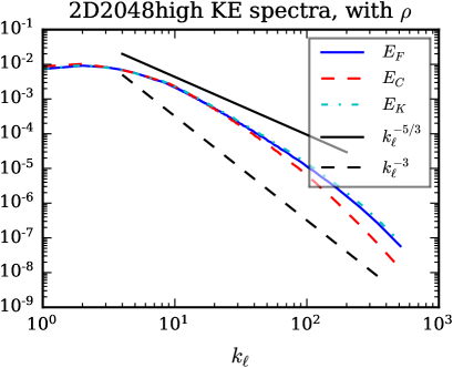
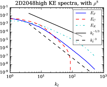
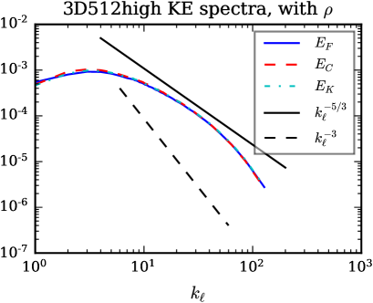
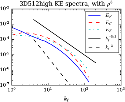
With , our flows have an initial density ratio of . Achieving higher ratios in a well-resolved turbulence simulation is computationally challenging, especially in 3D (e.g. \citeSuppLivescu08). Yet, many flows of interest have much larger density ratios, reaching of up to 600 laboratory flow experiments (\citeSuppRead84,DimonteSchneider00), typically exceeding in laboratory fusion plasmas (e.g. \citeSuppCraxtonetal15,Yan16,Zhangetal2020), and ranging from to in molecular clouds in the interstellar medium (e.g. \citeSuppKritsuketal07,Federrathetal10,Panetal16). The most ubiquitous terrestrial two-fluid mixing is between air and water which have a density ratio of 1000.
Since we are testing possible differences among the definitions, which can be applied to any density and velocity fields regardless of their dynamical origin, we synthetically increase the density contrast \citeSuppZhao18 in the flows we are analyzing by taking powers of the density, , as a post-processing step, then normalizing the resultant field such that the total mass in the domain is the same as in the original flow, . Note that this is not based on physical grounds, but serves to highlight differences among the three decompositions under higher density contrasts.
Figure S6 (right column) compares these three spectra using as a density field and original velocity from the high Atwood RT simulations in 2D and 3D. We now find more pronounced differences among the three decompositions, especially from the 2D2048high data; from equation (S-4) decays rapidly at high , while from equation (S-5) becomes shallower than the Favre-based spectrum (equation (S-3)), scaling similar to even in 2D.
The purpose of Figure S6 is to demonstrate that filtering spectra based on different kinetic energy decompositions can differ. It is not our intention here to argue which is more physical, which was the subject of previous studies (\citeSuppZhao18,Aluie13).
D 2D-RT simulation with same initial condition as in 3D1024
For verification purpose, we performed two additional 2D turbulent RT simulations (see Table 1); run 2D1024 of grid size and run 2D2048 on a grid. Both have the same initial perturbations as in 3D1024. Specifically, the vertical velocity field is perturbed at the interface in wavenumber space within the wavenumber annulus , with amplitude proportional to , where is a normalization constant to further limit the range of effectively perturbed wavenumber. We shall see that the analysis performed on these results are consistent with those obtained from run 2D4096 in the main text.
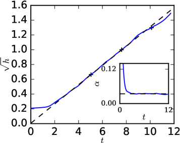
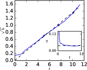
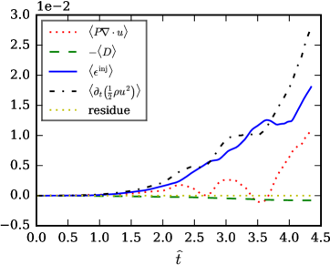
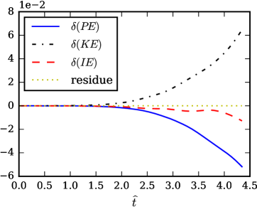
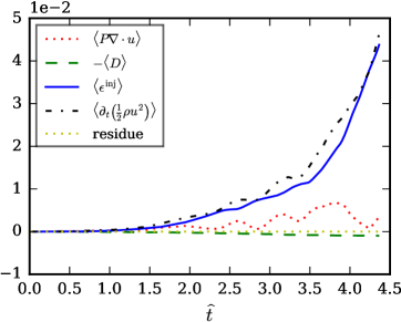
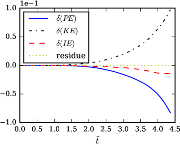
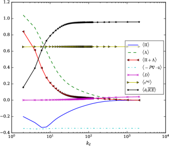
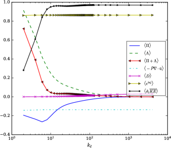
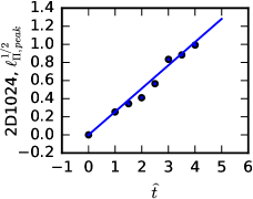
(a)
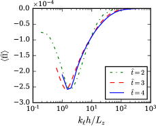
(b)
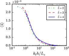
(c)
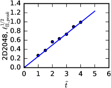
(d)
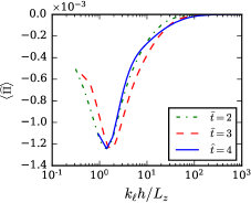
(e)
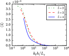
(f)
Figure S7 shows the mixing width versus time, with for 2D1024, and for 2D2048, which are similar to 2D4096 in figure 3 with . Figure S8 shows the corresponding instantaneous and overall kinetic energy budgets, which is similar to the 2D4096 case shown in figure 4(a) and 4(b). The KE budget as a function of scale is shown in figure S9, which resembles the 2D4096 result in figure 7 of the main text. The temporal self-similarity of the new 2D1024 and 2D2048 RT fluxes also holds, and is shown in figure S10, similar to those in the 2D4096 case in figure 11 of the main text. All the analysis presented here is consistent with the results from run 2D4096 in the main text, implying that the slight difference in initial conditions between 2D4096 and 3D1024 does not affect our conclusions.
E Another form of kinetic energy budget
In the compressible turbulence LES modeling literature, another formulation of the Favre filtered large scale kinetic energy budget, similar to equation (15) of the main text, is often used. In this formulation, pressure dilatation is lumped with the term by the relation:
| (S-6) |
using the identity (\citeSuppAluie11c)
Thus, the filtered large and small scale kinetic energy equations, and the filtered internal energy equation are:
| (S-7) | ||||
the omitted terms are similar to those in our formulation of the coarse-grained budgets in equation (15) of the main text. Many previous works on compressible turbulence adopt the framework of equation (S-7), see \citeSuppLele94 and the references therein. There are a few exceptions, such as in \citeSuppHuang95, in which they preferred to have a separate based on modelling considerations that density weighted decomposition should only be applied to the convective terms, and also in (\citeSuppAluie11c,Aluie13,Wang13,EyinkDrivas17a) where it was argued that and are fundamentally different from a physics standpoint since the former has contributions from scales both larger and smaller than and represents the interaction between different scales, while the latter only involves large scale quantities.
We remark that these two formulations, equation (15) of the main text and equation (S-7), are mathematically equivalent but represents different interpretations of the scale processes, which is illustrated schematically in figure S11 (in which potential energy and dissipation have been omitted for clarity). In figure S11, there are three channels for energy transfer: i) between internal energy (IE) and large scale kinetic energy (KE), ii) between IE and small scale KE, and iii) between large and small scale KE. For each channel, the energy transfer is different between the two interpretations, but the total energy transferred between IE and KE (when summing both large scales and small scales) is the same and equals to , as can be readily checked from the sum of the values associated with the arrows in both figures. However, an important distinction is that in the second formulation in figure 11(b), mean pressure dilatation acts over a much wider range of scales, preventing a simple understanding of the flow in terms of inertial range dynamics. This is illustrated with solid arrows in coupling internal energy to KE at scales both large and small, which can hinder the unraveling of inertial range dynamics. We thus advocate for using our formulation in equation (15) of the main text.
jfm \bibliographySuppRT_citation,Compressible_citation,Turbulence_citation,Numerical_citation
