Efficient MCMC Sampling for Bayesian Matrix Factorization by Breaking Posterior Symmetries

Abstract

Bayesian low-rank matrix factorization techniques have become an essential tool for relational data analysis and matrix completion. A standard approach is to assign zero-mean Gaussian priors on the columns or rows of factor matrices to create a conjugate system. This choice of prior leads to simple implementations; however it also causes symmetries in the posterior distribution that can severely reduce the efficiency of Markov-chain Monte-Carlo (MCMC) sampling approaches. In this paper, we propose a simple modification to the prior choice that provably breaks these symmetries and maintains/improves accuracy. Specifically, we provide conditions that the Gaussian prior mean and covariance must satisfy so the posterior does not exhibit invariances that yield sampling difficulties. For example, we show that using non-zero linearly independent prior means significantly lowers the autocorrelation of MCMC samples, and can also lead to lower reconstruction errors.

Keywords: Matrix completion, low-rank matrix factorization, Bayesian inference, posterior symmetry breaking, Markov chain Monte-Carlo (MCMC)

1 Introduction

The matrix completion problem seeks to use partial observations of a matrix to estimate missing entries. Formally, let $\mathbf{X}\in\mathbb{R}^{m\times n}$ be our target data matrix, and let $\Lambda\subseteq\{1,\ldots,m\}\times\{1,\ldots,n\}$ be a set of matrix indices where the matrix element is observed:

$$\bm{y}=\mathcal{P}_{\Lambda}(\mathbf{X})+\bm{\eta}.$$

Here, $\mathcal{P}_{\Lambda}:\mathbb{R}^{m\times n}\to\mathbb{R}^{\lvert\Lambda\rvert}$, $\lvert\Lambda\rvert$ being the cardinality of the set $\Lambda$, is the linear projection map

$$\mathcal{P}_{\Lambda}(\mathbf{X})=(x_{\bm{\lambda}}:\bm{\lambda}=(\lambda_{1},\lambda_{2})\in\Lambda),$$

and $\bm{\eta}\in\mathbb{R}^{\lvert\Lambda\rvert}$ is a vector of additive noises. Our goal is then to recover the matrix $\mathbf{X}$ from the observations $\bm{y}$. This problem commonly arises in many practical applications such as recommender system design (Takács et al., 2008), drug-target interaction prediction (Yamanishi et al., 2010; Zheng et al., 2013), image inpainting (He et al., 2015; Li et al., 2020), social network topology recovery (Mahindre et al., 2019) and sensor localization (Xue et al., 2019).

1.1 Related Works

This matrix problem is naturally ill-posed, and obtaining robust and accurate solutions requires imposing additional regularity conditions on the underlying data matrix such as sparsity or low-rank structures. In this paper, we consider the problem of low-rank matrix completion, where we might attempt to recover the matrix by nuclear norm minimization

$$\operatorname*{minimize}_{\mathbf{X}\in\mathbb{R}^{m\times n}}\quad\lVert\mathbf{X}\rVert_{*}\quad\text{subject to}\quad\lVert\bm{y}-\mathcal{P}_{\Lambda}(\mathbf{X})\rVert\leq\delta,$$ (1)

for some constant $\delta\geq 0$ that depends on the level of noise. Note that the nuclear norm is the convex relaxation of rank of a matrix (Candès and Recht, 2009), hence the objective in the optimization problem naturally encourages low-rank structure of the reconstruction. In Candès and Recht (2009), Candès and Tao (2010) and Candès and Plan (2010) the authors establish that, under mild assumptions about certain incoherence properties of $\mathbf{X}$, solving (1) leads to accurate recovery of the underlying data matrix with with surprisingly few observations. In fact, in absence of noise (that is, when $\bm{\eta}=\bm{0}$ and $\delta=0$) exact recovery is possible with high probability.

The standard solution method for optimization (1) is semi-definite programming, which is expensive when the matrix sizes $m$ and $n$ are large. In this setup, it is advantageous to explicitly use the low-rank factorization

$$\mathbf{X}=\mathbf{A}\mathbf{B}^{\top},\quad\mathbf{A}\in\mathbb{R}^{m\times r},\quad\mathbf{B}\in\mathbb{R}^{n\times r},\quad r\ll\min\{m,n\},$$ (2)

and solve the optimization problem

$$\operatorname*{minimize}_{\mathbf{A}\in\mathbb{R}^{m\times r},\mathbf{B}\in\mathbb{R}^{n\times r}}\quad\lVert\mathbf{A}\rVert_{F}^{2}+\lVert\mathbf{B}\rVert_{F}^{2}\quad\text{subject to}\quad\lVert\bm{y}-\mathcal{P}_{\Lambda}(\mathbf{A}\mathbf{B}^{\top})\rVert\leq\delta,$$ (3)

We can show that the optimization problems (1) and (3) are equivalent as long as the estimated rank $r$ is chosen to be larger than the true rank (Recht et al., 2010). We also consider the unconstrained version of (3):

$$\operatorname*{minimize}_{\mathbf{A}\in\mathbb{R}^{m\times r},\mathbf{B}\in\mathbb{R}^{n\times r}}\lVert\bm{y}-\mathcal{P}_{\Lambda}(\mathbf{A}\mathbf{B}^{\top})\rVert_{2}^{2}+\frac{\omega}{2}\lVert\mathbf{A}\rVert_{F}^{2}+\frac{\omega}{2}\lVert\mathbf{B}\rVert_{F}^{2}.$$ (4)

Generally speaking, these optimization-based approaches attempt to minimize the distance between the observed entries and their corresponding low-rank predictions while regularizing over the low-rank factors, and they serve as the base of a wide class of methods for low-rank matrix recovery (Srebro et al., 2005; Mnih and Salakhutdinov, 2008; Davenport and Romberg, 2016).

In this paper we instead focus on probabilistic approaches for which the solution also quantifies uncertainty in the predictions. Within this context the objective function (4) can easily be viewed as the negative log-posterior in a Bayesian parameter estimation problem with data $\bm{y}$ and parameters $\mathbf{A}$ and $\mathbf{B}$—it corresponds to i.i.d. zero-mean Gaussian priors on the entries of the factor matrices and observations corrupted by Gaussian noise. Lim and Teh (2007) and Raiko et al. (2007) each apply variational Bayes approximations of this inference model to analyze the Netflix prize challenge (Bennett et al., 2007) to great success. Further, Nakajima and Sugiyama (2011) and Nakajima et al. (2013) develop a theoretical framework to analyze the variational Bayes low-rank matrix factorization.

A fundamental issue with the variational Bayes approach lies in one of its modeling assumptions—namely the factors $\mathbf{A}$ and $\mathbf{B}$ are taken to be independent. Salakhutdinov and Mnih (2008) argues a fully Bayesian framework, which does not need this assumption, can outperform the variational models. Their proposed Markov-chain Monte-Carlo (MCMC) based approach is used in several later works (Chen et al., 2014; Ahn et al., 2015). More recently, it has been adapted for recovering low-rank tensor factorizations as well (Rai et al., 2014; Zhao et al., 2015a, b).

1.2 Our Contributions

In most of these variational and fully Bayesian inference setups, the priors and observations models are the same—they use Gaussian priors with zero means on the columns of the factor matrices, and assume observations are corrupted by additive Gaussian noise. One of the reason for the popularity of this choice of priors is rooted in the fact that it leads to simple analytical conditional posteriors, which is ideal for devising a Gibbs MCMC sampler (Alquier et al., 2014, 2015). Unfortunately, this choice of priors cannot fully mitigate the non-identifiability of the low-rank factorization (2)—given any $r\times r$ non-singular matrix $\mathbf{W}$ we can construct the new factors

$$\mathbf{\tilde{A}}=\mathbf{A}\mathbf{W}\text{ and }\mathbf{\tilde{B}}=\mathbf{B}\mathbf{W}^{-\top}\implies\mathbf{X}=\mathbf{\tilde{A}}\mathbf{\tilde{B}}^{\top}.$$

The effect of this invertible invariance shows up in the Bayes posteriors in the form of symmetries, as illustrated in Figure 2, where we plot the joint posterior between various components of the factor matrices, constructed from Hamiltonian Monte-Carlo (HMC) samples, for the fully observed $4\times 4$ rank-2 matrix described in Example 1 (Section 4). Effective MCMC sampling from distributions with such wide varying multi-modal and non-connected geometries is, in general, a difficult task.

Figure 1: Joint posterior between some components of the factor matrices. Results obtained using Hamiltonian Monte Carlo with zero mean priors.

Figure 2: Joint posterior between some components of the factor matrices (same as in Figure 2). Results obtained using Hamiltonian Monte Carlo, but this time with non-zero mean priors.

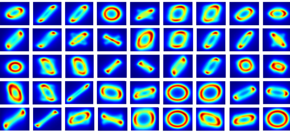
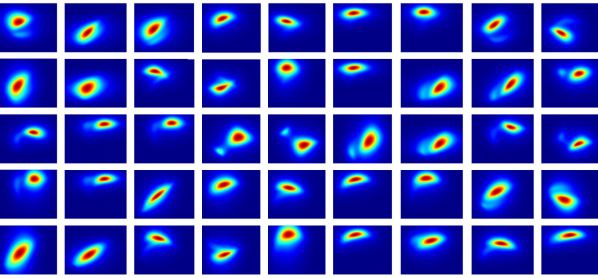
The main goal of this paper is to advocate a simple change in the prior specification, which does not break the local conjugacy required for Gibbs samplers, but breaks the posterior symmetries. Our contributions are threefold:

• In Theorem 3, we derive the exact conditions on the matrix $\mathbf{W}$ such that the posterior, assuming zero-mean Gaussian priors, is invariant under the transformation $(\mathbf{A},\mathbf{B})\mapsto(\mathbf{A}\mathbf{W},\mathbf{B}\mathbf{W}^{-\top})$.

• In Corollary 7 we prove that choosing a system of linearly independent prior means is sufficient for breaking this posterior symmetry. An illustration is given in Figure 2, where we plot the same set of joint posteriors as in Figure 2, but now constructed from HMC samples obtained with non-zero mean priors.

• By breaking the symmetry via introducing non-zero mean priors, we counter the non-identifiability of low-rank factorizations. We demonstrate this ultimately leads to better performance for MCMC sampling algorithms on matrices constructed from both synthetic and real-world data. We observe up to an order of magnitude decrease in the autocorrelations of generated samples and corresponding improvement in reconstruction errors of the underlying data matrices in our numerical examples in Section 4.

Note that our proposed change in prior means is very simple to implement—one needs to change at most a few lines of code in any existing applications. Constructing the appropriate prior means is also straightforward. From random matrix theory, we know that if the entries of a tall-and-thin matrix are sampled i.i.d. from any continuous random variable in $\mathbb{R}$, then the columns of the matrix form a linearly independent system with probability 1.

The rest of the paper is structured as follows. In Section 2, we formally introduce the Bayesian inference setup and quantify the symmetries arising from zero-mean Gaussian priors. In Section 3, we show that choosing the priors means to be non-zero in a systematic fashion breaks the invertible invariance. In Section 4, we present the numerical experiments. Finally, in Section 5, we present our concluding remarks and some directions for future work.

2 Notations and Bayesian Inference Setup

In this section, we introduce the notations we use throughout the rest of the paper, and introduce our Bayesian inference setup for the low-rank matrix factorization problem.

2.1 Notations

A vector $\bm{x}$ is always represented as a column, a row-vector is represented as $\bm{x}^{\top}$. The vector $\bm{e}_{i}$ is the $i$-th standard basis of appropriate (and inferable from context) size—all but its $i$-th entries are zero, and the non-zero entry is one.

Given a matrix $\mathbf{X}\in\mathbb{R}^{m\times n}$, we use $x_{ij}$ to denote its $(i,j)$-th entry. Additionally, $\bm{\bar{x}}_{i}\in\mathbb{R}^{n}$ and $\bm{x}_{j}\in\mathbb{R}^{m}$ denotes $i$-th row and the $j$-th column of the matrix; thus

$$\mathbf{X}=\begin{bmatrix}x_{11}&\cdots&x_{1n}\\ \vdots&\ddots&\vdots\\ x_{m1}&\cdots&x_{mn}\end{bmatrix}=\begin{bmatrix}\bm{x}_{1}&\cdots&\bm{x}_{n}\end{bmatrix}=\begin{bmatrix}\bm{\bar{x}}_{1}^{\top}\\ \vdots\\ \bm{\bar{x}}_{m}^{\top}\end{bmatrix}.$$

The matrix $\mathbf{I}_{n}$ denotes the $n\times n$ identity matrix.

We adopt MATLAB’s notation for indexing—given index sets $\Lambda_{r}\subseteq\{1,\ldots,m\}$ and $\Lambda_{c}\subseteq\{1,\ldots,n\}$ we use $\mathbf{X}[\Lambda_{r},\Lambda_{c}]$ to denote the intersection of the rows of $\mathbf{X}\in\mathbb{R}^{m\times n}$ indexed by $\Lambda_{r}$ and columns indexed by $\Lambda_{c}$. We also adopt the following slight abuses of notation:

$$\mathbf{X}[i,\Lambda_{c}] =\mathbf{X}[\{i\},\Lambda_{c}], \mathbf{X}[:,\Lambda_{c}] =\mathbf{X}[\{1,\ldots,m\},\Lambda_{c}],$$

$$\mathbf{X}[\Lambda_{r},j] =\mathbf{X}[\Lambda_{r},\{j\}], \mathbf{X}[\Lambda_{r},:] =\mathbf{X}[\Lambda_{r},\{1,\ldots,n\}].$$

2.2 Prior and Likelihood Models

Given a low-rank factorization (2), we impose independent Gaussian priors on the columns of the factor matrices

$$\bm{a}_{k}\sim\operatorname{\mathcal{N}}(\bm{\mu}_{a,k},\tau_{a,k}^{-1}\mathbf{I}_{m}),\quad\bm{b}_{k}\sim\operatorname{\mathcal{N}}(\bm{\mu}_{b,k},\tau_{b,k}^{-1}\mathbf{I}_{n}).$$

The joint prior is then given by

$$p(\mathbf{A},\mathbf{B})=\prod_{k=1}^{r}\operatorname{\mathcal{N}}(\bm{a}_{k}\mid\bm{\mu}_{a,k},\tau_{a,k}^{-1}\mathbf{I}_{m})\operatorname{\mathcal{N}}(\bm{b}_{k}\mid\bm{\mu}_{b,k},\tau_{b,k}^{-1}\mathbf{I}_{n}).$$

We assume real-valued matrices and a standard additive Gaussian noise model

$$y_{\bm{\lambda}}=x_{\bm{\lambda}}+\eta_{\bm{\lambda}},\quad\eta_{\bm{\lambda}}\sim\operatorname{\mathcal{N}}(0,\tau_{\eta}^{-1}),\quad\bm{\lambda}\in\Lambda.$$

Here $\Lambda$ is the set of location indices where the matrix was observed. The corresponding likelihood is given by

$$p(\bm{y}\mid\mathbf{A},\mathbf{B})=\prod_{\bm{\lambda}\in\Lambda}\operatorname{\mathcal{N}}(y_{\bm{\lambda}}\mid\bm{\bar{a}}_{\lambda_{1}}^{\top}\bm{\bar{b}}_{\lambda_{2}},\tau_{\eta}^{-1}).$$ (5)

The effect of invertible invariance of the likelihood is immediately obvious:

Proposition 1

The likelihood $p(\bm{y}\mid\mathbf{A},\mathbf{B})$ defined in (5) is invariant under invertible transformations. In particular, if $\mathbf{W}\in\mathbb{R}^{r\times r}$ is an invertible matrix, then

$$p(\bm{y}\mid\mathbf{A},\mathbf{B})=p(\bm{y}\mid\mathbf{A}\mathbf{W},\mathbf{B}\mathbf{W}^{-\top})\quad\text{for all}\quad\mathbf{A}\in\mathbb{R}^{m\times r}\text{ and }\mathbf{B}\in\mathbb{R}^{n\times r}.$$

Proof  Let $\mathbf{\tilde{A}}=\mathbf{A}\mathbf{W}$ and $\mathbf{\tilde{B}}=\mathbf{B}\mathbf{W}^{-\top}$. Then we note

$$\mathbf{\tilde{A}}\mathbf{\tilde{B}}^{\top}=(\mathbf{A}\mathbf{W})(\mathbf{B}\mathbf{W}^{-\top})^{\top}=\mathbf{A}\mathbf{W}\mathbf{W}^{-1}\mathbf{B}^{\top}=\mathbf{A}\mathbf{B}^{\top}.$$

Since all the matrix entries appearing in (5) are the same for both $(\mathbf{A},\mathbf{B})$ and $(\mathbf{\tilde{A}},\mathbf{\tilde{B}})$, it follows that the likelihood is invariant.  

2.3 The Posterior and its Symmetries

Using Bayes rule, the posterior is

$$p(\mathbf{A},\mathbf{B}\mid\bm{y})\propto p(\mathbf{A},\mathbf{B})p(\bm{y}\mid\mathbf{A},\mathbf{B})=p(\mathbf{A})p(\mathbf{B})p(\bm{y}\mid\mathbf{A},\mathbf{B}).$$

The negative log posterior is therefore

$$\begin{split}-\ln p(\mathbf{A},\mathbf{B}\mid\bm{y})&=\frac{mr}{2}\ln(2\pi)+\frac{m}{2}\sum_{k=1}^{r}\ln\frac{1}{\tau_{a,k}}+\frac{1}{2}\sum_{k=1}^{r}\tau_{a,k}\lVert\bm{a}_{k}-\bm{\mu}_{a,k}\rVert^{2}\\ &+\frac{nr}{2}\ln(2\pi)+\frac{n}{2}\sum_{k=1}^{r}\ln\frac{1}{\tau_{b,k}}+\frac{1}{2}\sum_{k=1}^{r}\tau_{b,k}\lVert\bm{b}_{k}-\bm{\mu}_{b,k}\rVert^{2}\\ &+\frac{\lvert\Lambda\rvert}{2}\ln(2\pi)+\frac{\lvert\Lambda\rvert}{2}\ln\frac{1}{\tau_{\eta}}+\frac{\tau_{\eta}}{2}\sum_{\bm{\lambda}\in\Lambda}(y_{\bm{\lambda}}-\bm{\bar{a}}_{\lambda_{1}}^{\top}\bm{\bar{b}}_{\lambda_{2}})^{2}+\text{const.}\end{split}$$ (6)

The first two lines correspond to the priors on $\mathbf{A}$ and $\mathbf{B}$, and the first three terms of the final line to the likelihood. The constant term corresponds to the evidence $p(\bm{y})$ of the observations, and can generally be ignored. We have already seen that the likelihood term is invariant under invertible transformations of the form $(\mathbf{A},\mathbf{B})\mapsto(\mathbf{A}\mathbf{W},\mathbf{B}\mathbf{W}^{-\top})$. Now we investigate any effect the prior terms might have. We immediately note the following:

Proposition 2

The posterior corresponding to (6) is invariant under invertible transformation $\mathbf{W}\in\mathbb{R}^{r\times r}$, i.e.

$$p(\mathbf{A},\mathbf{B}\mid\bm{y})=p(\mathbf{A}\mathbf{W},\mathbf{B}\mathbf{W}^{-\top}\mid\bm{y})\quad\text{for all}\quad\mathbf{A}\in\mathbb{R}^{m\times r}\text{ and }\mathbf{B}\in\mathbb{R}^{n\times r},$$

if and only if the terms

$$f_{1}(\mathbf{A}) =\sum_{k=1}^{r}\tau_{a,k}\lVert\bm{a}_{k}\rVert^{2}, f_{2}(\mathbf{A}) =\sum_{k=1}^{r}\tau_{a,k}\bm{\mu}_{a,k}^{\top}\bm{a}_{k},$$

$$f_{3}(\mathbf{B}) =\sum_{k=1}^{r}\tau_{b,k}\lVert\bm{b}_{k}\rVert^{2}, f_{4}(\mathbf{B}) =\sum_{k=1}^{r}\tau_{b,k}\bm{\mu}_{b,k}^{\top}\bm{b}_{k}$$

are individually invariant under the $\mathbf{A}\mapsto\mathbf{A}\mathbf{W}$ and $\mathbf{B}\mapsto\mathbf{B}\mathbf{W}^{-\top}$ transformations.

We can establish this result by essentially using the homogeneity of the $f_{1}$, $f_{2}$, $f_{3}$ and $f_{4}$ terms (a formal proof is presented in Appendix A). Clearly, the addition of prior imposes further restrictions on $\mathbf{W}$ for invertible invariance of the posterior (compared to the invariance of the likelihood). In particular, with zero-mean priors, the invariance exhibited by the likelihood under the transformation $(\mathbf{A},\mathbf{B})\mapsto(\mathbf{A}\mathbf{W},\mathbf{B}\mathbf{W}^{-\top})$ holds for the posterior only when $\mathbf{W}$ is restricted to a very particular subclass of invertible matrices:

Theorem 3 (Posterior symmetries with zero mean priors)

Let $\bm{\mu}_{a,k}=\bm{0}$ and $\bm{\mu}_{b,k}=\bm{0}$ for all $1\leq k\leq r$ and denote the diagonal matrices of the precision of the priors on the columns as

$$\mathbf{T}_{a}=\operatorname{diag}(\tau_{a,1},\ldots,\tau_{a,r}),\quad\mathbf{T}_{b}=\operatorname{diag}(\tau_{b,1},\ldots,\tau_{b,r}).$$

Let $\{\Lambda_{1},\ldots,\Lambda_{q}\}$ be a partition of $\{1,\ldots,r\}$ defined by the following:

$$k,k^{\prime}\in\Lambda_{\ell}\iff\tau_{a,k}\tau_{b,k}=\tau_{a,k^{\prime}}\tau_{b,k^{\prime}}.$$

Then the posterior corresponding to (6) is invariant under the $(\mathbf{A},\mathbf{B})\mapsto(\mathbf{A}\mathbf{W},\mathbf{B}\mathbf{W}^{-\top})$ transformation with invertible $\mathbf{W}\in\mathbb{R}^{r\times r}$ if and only if we can decompose

$$\mathbf{W}=\mathbf{T}_{a}^{1/2}\mathbf{Q}\mathbf{T}_{a}^{-1/2}=\mathbf{T}_{b}^{-1/2}\mathbf{Q}\mathbf{T}_{b}^{1/2},$$

where $\mathbf{Q}$ is orthogonal and block diagonal w.r.t. the partition $\{\Lambda_{1},\ldots,\Lambda_{q}\}$, i.e. the sub-matrices

$$\mathbf{Q}[\Lambda_{\ell_{1}},\Lambda_{\ell_{2}}]\text{ are }\begin{cases}\text{orthogonal}&\text{ if }\ell_{1}=\ell_{2}\\ \text{zero}&\text{ if }\ell_{1}\neq\ell_{2}\end{cases}.$$

We note that one direction of this theorem (that the above form of $\mathbf{W}$ is sufficient for the invariance of posterior) appears in Nakajima and Sugiyama (2011). We claim this structure of the matrix $\mathbf{W}$ is also necessary for invertible invariance as well; a formal proof is presented in Appendix B.

Two extreme cases of invariance with zero mean priors can be derived immediately from this theorem:

Corollary 4

Let $\bm{\mu}_{a,k}=\bm{0}$ and $\bm{\mu}_{b,k}=0$, $1\leq k\leq r$. Further suppose $\tau_{a,1}=\cdots=\tau_{a,r}$ and $\tau_{b,1}=\cdots=\tau_{b,r}$. Then the posterior corresponding to (6) is invariant under invertible transformation $\mathbf{W}$ if and only if $\mathbf{W}$ is orthogonal.

Proof  We have $\tau_{a,1}\tau_{b,1}=\cdots=\tau_{a,r}\tau_{b,r}$. Hence $\mathbf{Q}$ only has one block. Consequently invertible invariance holds if and only if $\mathbf{Q}$ is orthogonal (by Theorem 3). Additionally, we can write $\mathbf{T}_{a}=\tau_{a,1}\mathbf{I}_{r}$ where $\mathbf{I}_{r}$ is the $r\times r$ identity matrix. It follows that

$$\mathbf{W}=\mathbf{T}_{a}^{1/2}\mathbf{Q}\mathbf{T}_{a}^{-1/2}=\tau_{a,1}^{1/2}\mathbf{I}_{r}\mathbf{Q}\tau_{a,1}^{-1/2}\mathbf{I}_{r}=\mathbf{Q},$$

i.e. $\mathbf{Q}$ is orthogonal if and only if $\mathbf{W}$ is also orthogonal.  

Corollary 5

Let $\bm{\mu}_{a,k}=\bm{0}$ and $\bm{\mu}_{b,k}=0$, $1\leq k\leq r$. Further suppose $\tau_{a,1}\tau_{b,1},\ldots,\tau_{a,r}\tau_{b,r}$ are all distinct. Then the posterior corresponding to (6) is invariant under invertible transformation $\mathbf{W}$ if and only if $\mathbf{W}$ is diagonal with non-zero entries $\pm 1$.

Proof  It follows from Theorem 3 that $\mathbf{Q}$ must be block diagonal with block size $1$, and the each block has to be $\pm 1$ (these are the only $1\times 1$ orthogonal matrices). Let us write $\mathbf{Q}=\operatorname{diag}(q_{1},\ldots,q_{r})$ with each $q_{i}=\pm 1$. Then we have

$$\mathbf{W}=\operatorname{diag}(\tau_{a,1}^{1/2},\ldots,\tau_{a,r}^{1/2})\operatorname{diag}(q_{1},\ldots,q_{r})\operatorname{diag}(\tau_{a,1}^{-1/2},\ldots,\tau_{a,r}^{-1/2})=\operatorname{diag}(q_{1},\ldots,q_{r}).$$

It follows that invertible invariance holds if and only if $\mathbf{W}$ is diagonal with entries $\pm 1$.  

These corollaries make it clear that under zero-mean priors, there are at the very least $2^{r}$ symmetries in the posterior, corresponding to the $\mathbf{W}=\operatorname{diag}(\pm 1,\ldots,\pm 1)$ transformation matrices.

3 Breaking the Symmetries with Non-Zero Mean Priors

It is clear from Proposition 2 and Theorem 3 that the secret to completely breaking the symmetries can only hide in the $f_{2}$ and $f_{4}$ terms, which involve the prior means. This leads to our main result:

Theorem 6 (Breaking posterior symmetries)

Let $\mathbf{T}_{a}$, $\mathbf{T}_{b}$ and $\{\Lambda_{1},\ldots,\Lambda_{q}\}$ be as defined in the statement of Theorem 3. Define the prior mean matrices

$$\mathbf{M}_{a}=\begin{bmatrix}\bm{\mu}_{a,1}&\cdots&\bm{\mu}_{a,r}\end{bmatrix}\quad\text{and}\quad\mathbf{M}_{b}=\begin{bmatrix}\bm{\mu}_{b,1}&\cdots&\bm{\mu}_{b,r}\end{bmatrix}.$$

Then the posterior $p(\mathbf{A},\mathbf{B}\mid\bm{y})$ is not invariant under the $(\mathbf{A},\mathbf{B})\mapsto(\mathbf{A}\mathbf{W},\mathbf{B}\mathbf{W}^{-\top})$ transformation for any non-identity invertible $r\times r$ matrix $\mathbf{W}$ if and only if the matrices

$$\begin{bmatrix}\mathbf{M}_{a}[:,\Lambda_{\ell}]\mathbf{T}_{a}[\Lambda_{\ell},\Lambda_{\ell}]^{1/2}\\ \mathbf{M}_{b}[:,\Lambda_{\ell}]\mathbf{T}_{b}[\Lambda_{\ell},\Lambda_{\ell}]^{1/2}\end{bmatrix}$$ (7)

have full column rank for all $1\leq\ell\leq q$.

We postpone a formal proof until Appendix C; for now, we present an immediate corollary: it provides an extremely simple way to ensure full rank matrices (7). It essentially states that if the means are chosen to be linearly independent (e.g. the entries of the mean matrix are sampled i.i.d. from a zero-mean Gaussian distribution—the columns would be independent with probability 1), then the invariance is broken.

Corollary 7

Suppose either $\{\bm{\mu}_{a,k}:1\leq k\leq r\}$ or $\{\bm{\mu}_{b,k}:1\leq k\leq r\}$ form a linearly independent set in $\mathbb{R}^{m}$ or $\mathbb{R}^{n}$. Then the posterior $p(\mathbf{A},\mathbf{B}\mid\bm{y})$ is not invariant under any non-identity invertible transformations.

Proof  Suppose $\{\bm{\mu}_{a,k}:1\leq k\leq r\}$ is a linearly independent set in $\mathbb{R}^{m}$. Then $\mathbf{M}_{a}[:,\Lambda_{\ell}]$, and consequently $\mathbf{M}_{a}[:,\Lambda_{\ell}]\mathbf{T}_{a}[\Lambda_{\ell},\Lambda_{\ell}]^{1/2}$, are full rank for all $\ell$. It follows that

$$\mathbf{P}_{\ell}=\begin{bmatrix}\mathbf{M}_{a}[:,\Lambda_{\ell}]\mathbf{T}_{a}[\Lambda_{\ell},\Lambda_{\ell}]^{1/2}\\ \mathbf{M}_{b}[:,\Lambda_{\ell}]\mathbf{T}_{b}[\Lambda_{\ell},\Lambda_{\ell}]^{1/2}\end{bmatrix}$$

has full rank for all $\ell$, and Theorem 6 applies. A similar proof can be constructed when the prior means $\{\bm{\mu}_{b,k}:1\leq k\leq r\}$ form a linearly independent set in $\mathbb{R}^{n}$.  

Thus, by carefully choosing non-zero means for the priors on matrix factors, we can ensure that for any $r\times r$ invertible matrix $\mathbf{W}\neq\mathbf{I}$, the posteriors $p(\mathbf{A},\mathbf{B}\mid\bm{y})$ and $p(\mathbf{A}\mathbf{W}^{\top},\mathbf{B}\mathbf{W}^{-\top}\mid\bm{y})$ are distinct. In other words, with this choice of prior distributions, we can keep the identifiability issue from affecting Bayesian inference.

4 Numerical Results

We now demonstrate that symmetry breaking improves MCMC sampling, both in terms of efficiency (by decreasing autocorrelation) and accuracy (by reducing reconstruction error), with four numerical experiments. Examples 1 and 2 apply Bayesian matrix factorization with synthetic data, and Examples 3 and 4 work with real-world data. For each example, the entries of the non-zero prior mean matrices are sampled from a uniform distribution. We use the root mean squared error (RMSE) as a measure of error between the true matrix $\mathbf{X}\in\mathbb{R}^{m\times n}$ and its reconstruction $\hat{\mathbf{X}}\in\mathbb{R}^{m\times n}$:

$$\text{RMSE}=\sqrt{\frac{1}{mn}\sum_{i=1}^{m}\sum_{j=1}^{n}(x_{ij}-\hat{x}_{ij})^{2}}.$$

4.1 Example 1: Fully Observed Synthetic Matrix

We contrast the results obtained from running the HMC and Gibbs samplers on a rank-2 4$\times$4 matrix

$$\mathbf{X}=\begin{bmatrix}1&0&1&5\\ 2&-1&1&4\\ 4&-1&3&14\\ 3&-1&2&9\end{bmatrix},$$

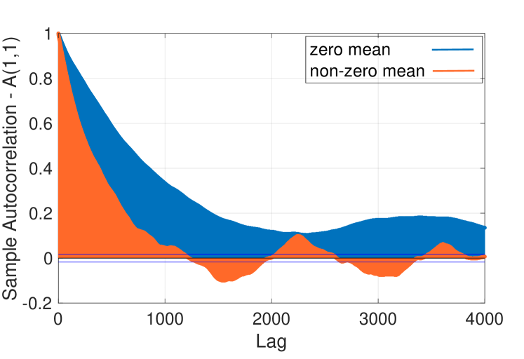
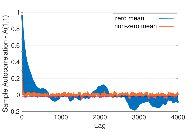
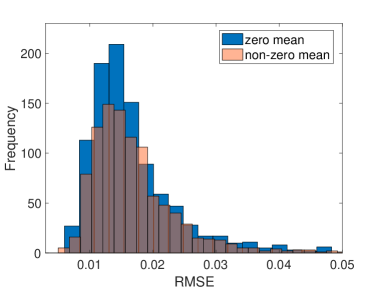
with zero and non-zero mean priors; the non-zero prior means $\mathbf{M}_{a}$ and $\mathbf{M}_{b}$ are constructed by sampling each of the entries from the $\text{Uniform}(0,1)$ distribution. We observe the full matrix with noise precision $\tau_{\eta}=10^{4}$, and MCMC results are obtained using both Gibbs and HMC samplers that use 10 chains, each with 20000 samples. We also assume that the precision is unknown, and follow the standard procedure of hierarchical Bayes by inferring the precision with prior $\tau_{\eta}\sim\text{Ga}(3,10^{-2})$. This leads to a conditionally conjugate posterior on $\tau_{\eta}$ (Alquier et al., 2014). In Figure 2 and Figure 2, we plot various joint posteriors, obtained using the samples generated using HMC, corresponding to the zero and non-zero mean priors. We can clearly see that the symmetries of the posterior in Figure 2 (corresponding to the zero mean priors) are not observed when using non-zero mean priors in Figure 2. This symmetry-breaking leads to better performance for MCMC samplers. For example, in Figure 4, we plot the autocorrelations for factor $a_{1,1}$ of the samples generated from both HMC and Gibbs samplers. The autocorrelations are significantly lower, for both samplers, when non-zero mean priors are used. This indicates using non-zero mean priors leads to better/faster mixing and smaller autocorrelations—regardless of algorithm used because the geometry of the posteriors are more favorable to the types of structures exploited by virtually all MCMC techniques. Further, in Figure 4, we plot the histogram of RMSE values of the matrix reconstruction for 1000 repetitions of the data gathering procedure—each experiment differs due to the noise realization and randomly sampled prior mean. For each of the repetitions we run 10 chains of the Gibbs sampler. Here the RMSE is on the order of $10^{-2}$ for both samplers—this is exactly what we expected because it is the order of the noise standard deviation. We can clearly see that, for this example, there is little difference in the RMSE based on the prior mean.

(a) Gibbs

(b) HMC

Figure 3: Autocorrelation for factor $a_{1,1}$ in Example 1 with zero and non-zero mean priors, computed using 10th chain of Gibbs and HMC samplers.

Figure 4: Reconstruction RMSE in Example 1 with zero and non-zero mean priors.

4.2 Example 2: Partially Observed Synthetic Matrix

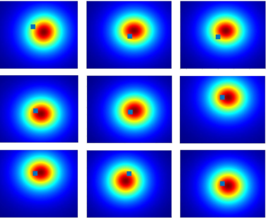
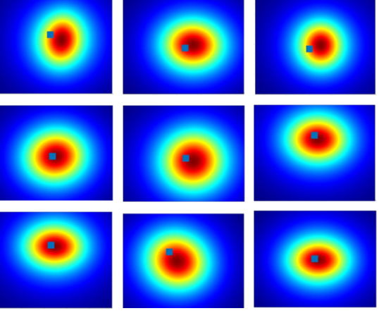
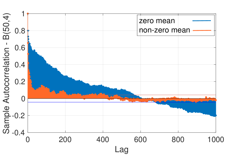
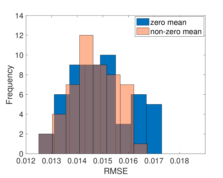
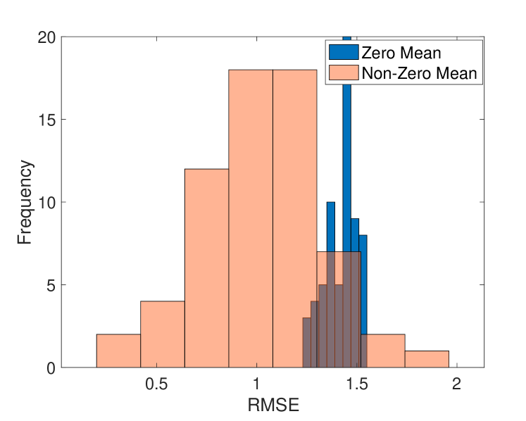
As we pointed out earlier, we often do not have access to observations of all entries of a matrix. To demonstrate the utility of our theory in context of partial observations, we use the Gibbs sampler to reconstruct a rank-5 $100\times 100$ matrix from observing only 20% of its entries. Sampling is performed with 5 chains, each with 5000 samples, and non-zero prior means are once again sampled from the $\text{Uniform}(0,1)$ distribution. The prior on the precision is the same as the previous example. We show the posterior predictions for some elements in Figure 7 corresponding to zero and non-zero mean priors; results are presented for same elements in Figure 7(a) and Figure 7(b). We can clearly see that using non-zero mean priors results in better MCMC performance. The corresponding order-of-magnitudes improvement in autocorrelation of the factor $b_{50,4}$ by choosing non-zero mean priors is showcased in Figure 7. The RMSE histogram constructed from 50 repetitions of the experiment is shown in Figure 7—here we see that using non-zero mean priors leads to better reconstruction errors.

(a) Zero mean priors

(b) Non-zero mean priors

Figure 5: Posterior predictions for some elements in Example 2 with Gibbs sampler. Blue marks indicate truth.

Figure 6: Autocorrelation for factor $b_{50,4}$ in Example 2 corresponding to zero and non-zero mean priors, computed with 5th chain of Gibbs sampler.

Figure 7: Reconstruction RMSE in Example 2 with zero and non-zero mean priors.

4.3 Example 3: Impaired Driving Dataset

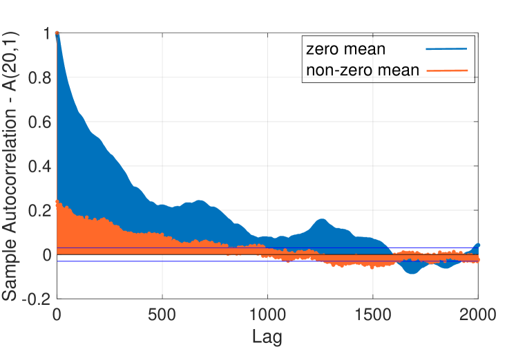
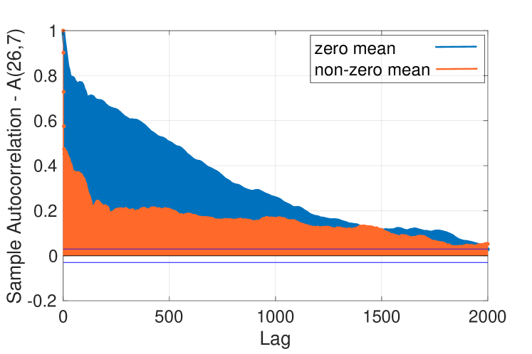
We now apply our theory to reconstruct the Impaired Driving Death Rate by Age and Gender data set available publicly from CDC. We assume 60% of the data is observed. Gibbs sampling is initiated with 5 chains, each with 10000 samples. Identical setup as in previous examples is used for this experiment. We demonstrate that introducing non-zero mean priors improves the autocorrelation for the $a_{20,1}$ and $a_{26,7}$ in Figure 8. Again we see significant improvement in efficiency in the same MCMC sampler.

(a) Factor $a_{20,1}$

(b) Factor $a_{26,7}$

Figure 8: Autocorrelation for some factors in Example 3 corresponding to zero and non-zero mean priors, computed from 3rd chain of Gibbs sampler.

4.4 Example 4: Mice Protein Expression Dataset

Finally, we apply our theory to the mice-protein expression data set (Higuera et al., 2015) available from the UCI Machine Learning Repository. The data set consists of 77 protein expressions, measured in terms of nuclear fractions, from 1080 mice specimens. For our experiments, we randomly sub-sampled this $1080\times 77$ matrix, creating a $50\times 50$ fully-observed sub-matrix. We then constructed a rank 10 factorization of the form (2) using Gibbs sampling while observing only 50% of the entries. Sampling was initiated for 4 chains, each with 20000 samples. We set the parameter values

$$\tau_{a,1}=\cdots=\tau_{a,10}=25,\quad\tau_{b,1}=\cdots=\tau_{b,10}=25,\quad\tau_{\eta}=10^{2},$$

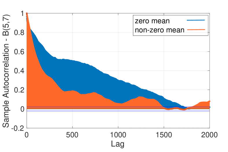
and the entries of the non-zero prior mean matrices were sampled from the $\text{Uniform}(-\frac{7}{2},\frac{7}{2})$ distribution. The first 1000 samples from all chains were discarded as burn-in. We observe that using non-zero mean priors leads to improvement of sample autocorrelation for the $b_{5,7}$ factor in Figure 10. We also see improved reconstruction errors in Figure 10—the RMSE histograms were computed from 64 independent repetitions of the experiment described above, with ten-fold sample thinning.

Figure 9: Autocorrelation for factor $b_{5,7}$ in Example 4 corresponding to zero/non-zero means, computed from 4th chain of Gibbs sampler.

Figure 10: Reconstruction RMSE in Example 4 from 64 Gibbs sampling experiments with zero and non-zero mean priors.

5 Conclusion

We have presented a full theoretical treatment of the symmetries of posteriors that arise from non-identifiability in Bayesian low-rank matrix factorization due to the standard choice of Gaussian priors on the matrix factors. We established that using a carefully chosen set of prior means, we can eliminate these symmetries, leading to better performance of MCMC sampling algorithms both with synthetic and real-world data. In future, we intend to extend this framework to address similar non-identifiability issues for low-rank tensor factorizations.

Acknowledgments

S. De acknowledges support from NSF under grant DMS-1454010 and from the Automotive Research Center (ARC) in accordance with Cooperative Agreement W56HZV-14-2-0001 with U.S. Army Ground Vehicle Systems Center.

A. Gorodetsky and H. Salehi acknowledge support from the Department of Energy Office of Scientific Research, ASCR under grant DE-SC0020364.

A Proof of Proposition 2

Proposition 2 The posterior corresponding to

$$\begin{split}-\log p(\mathbf{A},\mathbf{B}\mid\bm{y})=\frac{1}{2}\sum_{k=1}^{r}\tau_{a,k}\lVert\bm{a}_{k}-\bm{\mu}_{a,k}\rVert^{2}&+\frac{1}{2}\sum_{k=1}^{r}\tau_{b,k}\lVert\bm{b}_{k}-\bm{\mu}_{b,k}\rVert^{2}\\ &+\frac{\tau_{\eta}}{2}\sum_{\bm{\lambda}\in\Lambda}(y_{\bm{\lambda}}-\bm{\bar{a}}_{\lambda_{1}}^{\top}\bm{\bar{b}}_{\lambda_{2}})^{2}+\text{const.}\end{split}$$

is invariant under invertible transformation $\mathbf{W}\in\mathbb{R}^{r\times r}$, i.e.

$$p(\mathbf{A},\mathbf{B}\mid\bm{y})=p(\mathbf{A}\mathbf{W},\mathbf{B}\mathbf{W}^{-\top}\mid\bm{y})\quad\text{for all}\quad\mathbf{A}\in\mathbb{R}^{m\times r}\text{ and }\mathbf{B}\in\mathbb{R}^{n\times r},$$

if and only if the terms

$$f_{1}(\mathbf{A}) =\sum_{k=1}^{r}\tau_{a,k}\lVert\bm{a}_{k}\rVert^{2}, f_{2}(\mathbf{A}) =\sum_{k=1}^{r}\tau_{a,k}\bm{\mu}_{a,k}^{\top}\bm{a}_{k},$$

$$f_{3}(\mathbf{B}) =\sum_{k=1}^{r}\tau_{b,k}\lVert\bm{b}_{k}\rVert^{2}, f_{4}(\mathbf{B}) =\sum_{k=1}^{r}\tau_{b,k}\bm{\mu}_{b,k}^{\top}\bm{b}_{k}$$

are individually invariant under the $\mathbf{A}\mapsto\mathbf{A}\mathbf{W}$ and $\mathbf{B}\mapsto\mathbf{B}\mathbf{W}^{-\top}$ transformations.

Proof  Note that

$$\lVert\bm{a}_{k}-\bm{\mu}_{a,k}\rVert^{2}=\lVert\bm{a}_{k}\rVert^{2}-2\bm{\mu}_{a,k}^{\top}\bm{a}_{k}+\text{const.},$$

and similarly

$$\lVert\bm{b}_{k}-\bm{\mu}_{b,k}\rVert^{2}=\lVert\bm{b}_{k}\rVert^{2}-2\bm{\mu}_{b,k}^{\top}\bm{b}_{k}+\text{const.}$$

Thus, we can rewrite the negative log posterior as

$$-\log p(\mathbf{A},\mathbf{B}\mid\bm{y})=\frac{1}{2}f_{1}(\mathbf{A})-f_{2}(\mathbf{A})+\frac{1}{2}f_{3}(\mathbf{B})-f_{4}(\mathbf{B})-\log p(\bm{y}\mid\mathbf{A},\mathbf{B})+\text{const.}$$ (8)

From Proposition 1, we see that the likelihood term is already invariant under the invertible transformation. It follows invariance of $f_{1}$, $f_{2}$, $f_{3}$ and $f_{4}$ is sufficient for invariance of the posterior.

We now establish that invariance of $f_{1}$, $f_{2}$, $f_{3}$ and $f_{4}$ is necessary for invariance of the posterior. To show this, first note that $f_{1}$, $f_{3}$ are homogeneous of degree two, and $f_{2}$, $f_{4}$ are homogeneous of degree one. More explicitly, for all $t,s\in\mathbb{R}$ we have

$$f_{1}(t\mathbf{A}) =t^{2}f_{1}(\mathbf{A}), f_{2}(t\mathbf{A}) =tf_{2}(\mathbf{A}),$$

$$f_{3}(s\mathbf{B}) =s^{2}f_{3}(\mathbf{B}), f_{4}(s\mathbf{B}) =sf_{4}(\mathbf{B}).$$

Now, fix $\mathbf{A}$ and $\mathbf{B}$, then for invariance we must have $p(t\mathbf{A},s\mathbf{B}\mid\bm{y})=p(t\mathbf{A}\mathbf{W},s\mathbf{B}\mathbf{W}^{-\top}\mid\bm{y})$ for all $s,t\in\mathbb{R}$. Expanding this out using (8) and applying the homogeneity properties, we obtain

$$\frac{t^{2}}{2}f_{1}(\mathbf{A})-tf_{2}(\mathbf{A})+\frac{s^{2}}{2}f_{3}(\mathbf{B})-sf_{4}(\mathbf{B})=\frac{t^{2}}{2}f_{1}(\mathbf{A}\mathbf{W})-tf_{2}(\mathbf{A}\mathbf{W})+\frac{s^{2}}{2}f_{3}(\mathbf{B}\mathbf{W}^{-\top})-sf_{4}(\mathbf{B}\mathbf{W}^{-\top}),$$

where the likelihood term cancels out. Comparing the coefficients of like-powered terms on the both sides, we conclude that we must have

$$f_{1}(\mathbf{A}) =f_{1}(\mathbf{A}\mathbf{W}) f_{2}(\mathbf{A}) =f_{2}(\mathbf{A}\mathbf{W})$$

$$f_{3}(\mathbf{B}) =f_{3}(\mathbf{B}\mathbf{W}^{-\top}) f_{4}(\mathbf{B}) =f_{4}(\mathbf{B}\mathbf{W}^{-\top})$$

Since $\mathbf{A}$ and $\mathbf{B}$ are arbitrary, it follows that $f_{1}$, $f_{2}$, $f_{3}$ and $f_{4}$ must be individually invariant under the $\mathbf{A}\mapsto\mathbf{A}\mathbf{W}$ and $\mathbf{B}\mapsto\mathbf{B}\mathbf{W}^{-\top}$ transformations.  

B Proof of Theorem 3

We will use the following result:

Lemma 8

Let $\mathbf{Q}\in\mathbb{R}^{r\times r}$ be a matrix satisfying $\lVert\mathbf{Q}\bm{x}\rVert=\lVert\bm{x}\rVert$ for all $\bm{x}\in\mathbb{R}^{r}$. Then $\mathbf{Q}$ is orthogonal.

Proof  Let $\bm{x}_{1}$ and $\bm{x}_{2}$ be two arbitrary vectors. Then

$$\lVert\mathbf{Q}\bm{x}_{1}+\mathbf{Q}\bm{x}_{2}\rVert^{2}=\lVert\mathbf{Q}\bm{x}_{1}\rVert^{2}+\lVert\mathbf{Q}\bm{x}_{2}\rVert^{2}+2\langle\mathbf{Q}\bm{x}_{1},\mathbf{Q}\bm{x}_{2}\rangle$$

and

$$\lVert\bm{x}_{1}+\bm{x}_{2}\rVert^{2}=\lVert\bm{x}_{1}\rVert^{2}+\lVert\bm{x}_{2}\rVert^{2}+2\langle\bm{x}_{1},\bm{x}_{2}\rangle$$

Using the facts $\lVert\mathbf{Q}\bm{x}_{1}+\mathbf{Q}\bm{x}_{2}\rVert=\lVert\mathbf{Q}(\bm{x}_{1}+\bm{x}_{2})\rVert=\lVert\bm{x}_{1}+\bm{x}_{2}\rVert$, $\lVert\mathbf{Q}\bm{x}_{1}\rVert=\lVert\bm{x}_{1}\rVert$ and $\lVert\mathbf{Q}\bm{x}_{2}\rVert=\lVert\bm{x}_{2}\rVert$ we obtain

$$\langle\mathbf{Q}\bm{x}_{1},\mathbf{Q}\bm{x}_{2}\rangle=\langle\bm{x}_{1},\bm{x}_{2}\rangle\quad\text{for all}\quad\bm{x}_{1},\bm{x}_{2}\in\mathbb{R}^{r}$$

Setting $\bm{x}_{1}=\bm{e}_{i}$ and $\bm{x}_{2}=\bm{e}_{j}$, we obtain

$$\langle\bm{q}_{i},\bm{q}_{j}\rangle=\langle\bm{e}_{i},\bm{e}_{j}\rangle$$

i.e. $\{\bm{q}_{1},\ldots,\bm{q}_{r}\}$ form an orthonormal system in $\mathbb{R}^{r}$, hence $\mathbf{Q}$ is orthogonal.  

For convenience, we restate Theorem 3 slightly differently than earlier:

Theorem 3 Let us denote

$$\mathbf{T}_{a}=\operatorname{diag}(\tau_{a,1},\ldots,\tau_{a,r}),\quad\mathbf{T}_{b}=\operatorname{diag}(\tau_{b,1},\ldots,\tau_{b,r})$$

Let $\{\Lambda_{1},\ldots,\Lambda_{q}\}$ be a partition of $\{1,\ldots,r\}$ defined by the equivalence relation

$$k,k^{\prime}\in\Lambda_{\ell}\iff\tau_{a,k}\tau_{b,k}=\tau_{a,k^{\prime}}\tau_{b,k^{\prime}}$$

Then the posterior given by

$$-\log p(\mathbf{A},\mathbf{B}\mid\bm{y})=\frac{1}{2}\sum_{k=1}^{r}\tau_{a,k}\lVert\bm{a}_{k}\rVert^{2}+\frac{1}{2}\sum_{k=1}^{r}\tau_{b,k}\lVert\bm{b}_{k}\rVert^{2}+\frac{\tau_{\eta}}{2}\sum_{\bm{\lambda}\in\Lambda}(y_{\bm{\lambda}}-\bm{\bar{a}}_{\lambda_{1}}^{\top}\bm{\bar{b}}_{\lambda_{2}})^{2}+\text{const.}$$ (9)

is invariant under transformation $(\mathbf{A},\mathbf{B})\mapsto(\mathbf{A}\mathbf{W},\mathbf{B}\mathbf{W}^{-\top})$ with invertible $\mathbf{W}\in\mathbb{R}^{r\times r}$ if and only if we can decompose

$$\mathbf{W}=\mathbf{T}_{a}^{1/2}\mathbf{Q}\mathbf{T}_{a}^{-1/2}=\mathbf{T}_{b}^{-1/2}\mathbf{Q}\mathbf{T}_{b}^{1/2}$$ (10)

where $\mathbf{Q}$ is orthogonal and block diagonal w.r.t. the partition $\{\Lambda_{1},\ldots,\Lambda_{q}\}$, i.e. the sub-matrices

$$\mathbf{Q}[\Lambda_{\ell_{1}},\Lambda_{\ell_{2}}]\text{ are }\begin{cases}\text{orthogonal}&\text{ if }\ell_{1}=\ell_{2}\\ \text{zero}&\text{ if }\ell_{1}\neq\ell_{2}\end{cases}$$ (11)

Proof  From Proposition 2, invertible invariance (9) holds if and only if the terms

$$f_{1}(\mathbf{A})=\sum_{k=1}^{r}\tau_{a,k}\lVert\bm{a}_{k}\rVert^{2},\quad f_{3}(\mathbf{B})=\sum_{k=1}^{r}\tau_{b,k}\lVert\bm{b}_{k}\rVert^{2}$$

are invariant under the $\mathbf{A}\mapsto\mathbf{A}\mathbf{W}$ and $\mathbf{B}\mapsto\mathbf{B}\mathbf{W}^{-\top}$ transformations.

We divide the rest of the proof into three steps:

• Step 1 derives the following condition on $\mathbf{W}$ necessary for invertible invariance:

  $$\mathbf{Q}_{a}=\mathbf{T}_{a}^{-1/2}\mathbf{W}\mathbf{T}_{a}^{1/2}\quad\text{and}\quad\mathbf{Q}_{b}=\mathbf{T}_{b}^{1/2}\mathbf{W}\mathbf{T}_{b}^{-1/2}$$ (12)

  must be orthogonal matrices.

• Step 2 establishes $\mathbf{Q}_{a}=\mathbf{Q}_{b}$, and derives the block diagonal structure (11) on this common orthogonal matrix $\mathbf{Q}$. This establishes (10) as a necessary condition for invertible invariance.

• Step 3 proves that (10) is in fact sufficient for invertible invariance.

Step 1. Let us choose

$$\mathbf{A}=\begin{bmatrix}\alpha_{1}&\cdots&\alpha_{r}\\ 0&\cdots&0\\ \vdots&\ddots&\vdots\\ 0&\cdots&0\end{bmatrix}_{m\times r}\implies\mathbf{A}\mathbf{W}=\begin{bmatrix}\bm{\alpha}^{\top}\\ \bm{0}^{\top}\\ \vdots\\ \bm{0}^{\top}\end{bmatrix}\begin{bmatrix}\bm{w}_{1}&\cdots&\bm{w}_{r}\end{bmatrix}=\begin{bmatrix}\bm{\alpha}^{\top}\bm{w}_{1}&\cdots&\bm{\alpha}^{\top}\bm{w}_{r}\\ 0&\cdots&0\\ \vdots&\ddots&\vdots\\ 0&\cdots&0\end{bmatrix}_{m\times r}$$

for arbitrary $\bm{\alpha}\in\mathbb{R}^{r}$. Then we have

$$f(\mathbf{A}) =\sum_{k=1}^{r}\tau_{a,k}\alpha_{k}^{2}=\lVert\mathbf{T}_{a}^{1/2}\bm{\alpha}\rVert^{2}$$

$$f(\mathbf{A}\mathbf{W}) =\sum_{k=1}^{r}\tau_{a,k}(\bm{\alpha}^{\top}\bm{w}_{k})^{2}=\sum_{k=1}^{r}\tau_{a,k}(\bm{w}_{k}^{\top}\bm{\alpha})^{2}=\lVert\mathbf{T}_{a}^{1/2}\mathbf{W}^{\top}\bm{\alpha}\rVert^{2}$$

These equalities follow from the following observations:

$$\mathbf{T}_{a}^{1/2}\bm{\alpha}=\begin{bmatrix}\tau_{a,1}^{1/2}\alpha_{1}\\ \vdots\\ \tau_{a,r}^{1/2}\alpha_{r}\end{bmatrix},\quad\mathbf{T}_{a}^{1/2}\mathbf{W}^{\top}\bm{\alpha}=\mathbf{T}_{a}^{1/2}\begin{bmatrix}\bm{w}_{1}^{\top}\bm{\alpha}\\ \vdots\\ \bm{w}_{r}^{\top}\bm{\alpha}\end{bmatrix}=\begin{bmatrix}\tau_{a,1}^{1/2}\bm{w}_{1}^{\top}\bm{\alpha}\\ \vdots\\ \tau_{a,r}^{1/2}\bm{w}_{r}^{\top}\bm{\alpha}\end{bmatrix}$$

Thus, invariance of $f_{1}$ under $\mathbf{A}\mapsto\mathbf{A}\mathbf{W}$ transformation requires

$$\lVert\mathbf{T}_{a}^{1/2}\bm{\alpha}\rVert=\lVert\mathbf{T}_{a}^{1/2}\mathbf{W}^{\top}\bm{\alpha}\rVert\quad\text{for all}\quad\bm{\alpha}\in\mathbb{R}^{r}$$

Set $\bm{\beta}=\mathbf{T}_{a}^{1/2}\bm{\alpha}$, then by the invertibility of $\mathbf{T}_{a}$ we can rewrite this condition as

$$\lVert\bm{\beta}\rVert=\lVert\underbrace{\mathbf{T}_{a}^{1/2}\mathbf{W}^{\top}\mathbf{T}_{a}^{-1/2}}_{\mathbf{Q}_{a}^{\top}}\bm{\beta}\rVert\quad\text{for all}\quad\bm{\beta}\in\mathbb{R}^{r}$$

Lemma 8 then implies that $\mathbf{Q}_{a}^{\top}$, and consequently $\mathbf{Q}_{a}$ (as defined in (12)), must be orthogonal. Proceeding in a similar manner, we can show that the invariance of $f_{3}$ under the $\mathbf{B}\mapsto\mathbf{B}\mathbf{W}^{-\top}$ transformation would require $\mathbf{Q}_{b}$ (again, as defined in (12)) to be orthogonal.

Step 2. Using (12) we can compute

$$\mathbf{Q}_{a}^{-1}=\mathbf{T}_{a}^{-1/2}\mathbf{W}^{-1}\mathbf{T}_{a}^{1/2}\implies\mathbf{Q}_{a}^{-\top}=\mathbf{T}_{a}^{1/2}\mathbf{W}^{-\top}\mathbf{T}_{a}^{-1/2}$$

But since $\mathbf{Q}_{a}$ is orthogonal we have

$$\mathbf{Q}_{a}=\mathbf{Q}_{a}^{-\top}\implies\mathbf{T}_{a}^{-1/2}\mathbf{W}\mathbf{T}_{a}^{1/2}=\mathbf{T}_{a}^{1/2}\mathbf{W}^{-\top}\mathbf{T}_{a}^{-1/2}\implies\mathbf{W}\mathbf{T}_{a}=\mathbf{T}_{a}\mathbf{W}^{-\top}$$ (13)

Similarly, from (12) and orthogonality of $\mathbf{Q}_{b}$, we can derive

$$\mathbf{T}_{b}\mathbf{W}=\mathbf{W}^{-\top}\mathbf{T}_{b}$$ (14)

Using (13) and (14) along with associativity of matrix multiplication, we obtain

$$\mathbf{T}_{a}\mathbf{T}_{b}\mathbf{W}=\mathbf{T}_{a}(\mathbf{T}_{b}\mathbf{W})\overset{\eqref{eq:posterior-symmetry-eq-2}}{=}\mathbf{T}_{a}(\mathbf{W}^{-\top}\mathbf{T}_{b})=(\mathbf{T}_{a}\mathbf{W}^{-\top})\mathbf{T}_{b}\overset{\eqref{eq:posterior-symmetry-eq-1}}{=}(\mathbf{W}\mathbf{T}_{a})\mathbf{T_{b}}=\mathbf{W}\mathbf{T}_{a}\mathbf{T}_{b}$$

Now, equating $(i,j)$-th entries of the two boundary matrices in the above chain (which are easy to compute given diagonal $\mathbf{T}_{a}$ and $\mathbf{T}_{b}$), we get

$$\tau_{a,i}\tau_{b,i}w_{ij}=w_{ij}\tau_{a,j}\tau_{b,j}\quad\text{for all}\quad 1\leq i,j\leq r$$

Clearly, if $\tau_{a,i}\tau_{b,i}\neq\tau_{a,j}\tau_{b,j}$ for some pair of indices $(i,j)$, then we must have $w_{ij}=0$. This leads us to the block-diagonal structure of $\mathbf{W}$ w.r.t. partition $\{\Lambda_{1},\ldots,\Lambda_{q}\}$, i.e. $\mathbf{W}[\Lambda_{\ell_{1}},\Lambda_{\ell_{2}}]$ is non-zero only if $\ell_{1}=\ell_{2}$. Using this with the diagonal nature of $\mathbf{T}_{a}$ and $\mathbf{T}_{b}$ in (12), we can conclude $\mathbf{Q}_{a}$ and $\mathbf{Q}_{b}$ have the same block-diagonal structure.

Next, for each $1\leq\ell\leq q$ we have $\tau_{a,i}\tau_{b,i}=\tau_{a,j}\tau_{b,j}$ for all $i,j\in\Lambda_{\ell}$. Let us call this common value $c_{\ell}$, then we have

$$\begin{split}\mathbf{T}_{a}[\Lambda_{\ell},\Lambda_{\ell}]\mathbf{T}_{b}[\Lambda_{\ell},\Lambda_{\ell}]&=\operatorname{diag}(\tau_{a,i}:i\in\Lambda_{\ell})\operatorname{diag}(\tau_{b,i}:i\in\Lambda_{\ell})\\ &=\operatorname{diag}(\tau_{a,i}\tau_{b,i}:i\in\Lambda_{\ell})\\ &=\operatorname{diag}(c_{\ell}:i\in\Lambda_{\ell})\\ &=c_{\ell}\mathbf{I}_{r_{\ell}}\end{split}$$

where we denote $r_{\ell}=\lvert\Lambda_{\ell}\rvert$. We conclude

$$\begin{split}\mathbf{T}_{b}[\Lambda_{\ell},\Lambda_{\ell}]&=c_{\ell}\mathbf{T}_{a}[\Lambda_{\ell},\Lambda_{\ell}]^{-1}\\ \implies\mathbf{Q}_{b}[\Lambda_{\ell},\Lambda_{\ell}]&=\mathbf{T}_{b}[\Lambda_{\ell},\Lambda_{\ell}]^{1/2}\mathbf{W}[\Lambda_{\ell},\Lambda_{\ell}]\mathbf{T}_{b}[\Lambda_{\ell},\Lambda_{\ell}]^{-1/2}\\ &=c_{\ell}^{1/2}\mathbf{T}_{a}[\Lambda_{\ell},\Lambda_{\ell}]^{-1/2}\mathbf{W}[\Lambda_{\ell},\Lambda_{\ell}]c_{\ell}^{-1/2}\mathbf{T}_{a}[\Lambda_{\ell},\Lambda_{\ell}]^{1/2}\\ &=\mathbf{T}_{a}[\Lambda_{\ell},\Lambda_{\ell}]^{-1/2}\mathbf{W}[\Lambda_{\ell},\Lambda_{\ell}]\mathbf{T}_{a}[\Lambda_{\ell},\Lambda_{\ell}]^{1/2}\\ &=\mathbf{Q}_{a}[\Lambda_{\ell},\Lambda_{\ell}]\end{split}$$

Combining these for all the blocks, we obtain $\mathbf{Q}_{a}=\mathbf{Q}_{b}$. We call this common value $\mathbf{Q}$, and (10) is trivially satisfied.

Step 3. This part of the proof is taken from Nakajima and Sugiyama (2011, Appendix G.3):

Note that we can write

$$f_{1}(\mathbf{A})=\sum_{k=1}^{r}\tau_{a,k}\lVert\bm{a}_{k}\rVert^{2}=\operatorname{trace}((\mathbf{T}_{a}\mathbf{A}^{\top})\mathbf{A})=\operatorname{trace}(\mathbf{A}(\mathbf{T}_{a}\mathbf{A}^{\top}))=\operatorname{trace}(\mathbf{A}\mathbf{T}_{a}\mathbf{A}^{\top})$$

where the second equality follows from the following observation:

$$\begin{split}(\mathbf{T}_{a}\mathbf{A}^{\top})\mathbf{A}&=\left(\begin{bmatrix}\tau_{a,1}&&\\ &\ddots&\\ &&\tau_{a,r}\end{bmatrix}\begin{bmatrix}\bm{a}_{1}^{\top}\\ \vdots\\ \bm{a}_{r}^{\top}\end{bmatrix}\right)\begin{bmatrix}\bm{a}_{1}&\cdots&\bm{a}_{r}\end{bmatrix}\\ &=\begin{bmatrix}\tau_{a,1}\bm{a}_{1}^{\top}\\ \vdots\\ \tau_{a,r}\bm{a}_{r}^{\top}\end{bmatrix}\begin{bmatrix}\bm{a}_{1}&\cdots&\bm{a}_{r}\end{bmatrix}\\ &=\begin{bmatrix}\tau_{a,1}\bm{a}_{1}^{\top}\bm{a}_{1}&\cdots&\tau_{a,1}\bm{a}_{1}^{\top}\bm{a}_{r}\\ \vdots&\ddots&\vdots\\ \tau_{a,1}\bm{a}_{r}^{\top}\bm{a}_{1}&\cdots&\tau_{a,1}\bm{a}_{r}^{\top}\bm{a}_{r}\end{bmatrix}\end{split}$$

Now, using $\mathbf{W}=\mathbf{T}_{a}^{1/2}\mathbf{Q}\mathbf{T}_{a}^{-1/2}$ from (10), we get

$$\begin{split}f_{1}(\mathbf{A}\mathbf{W})&=\operatorname{trace}((\mathbf{A}\mathbf{W})\mathbf{T}_{a}(\mathbf{A}\mathbf{W})^{\top})\\ &=\operatorname{trace}(\mathbf{A}\mathbf{W}\mathbf{T}_{a}\mathbf{W}^{\top}\mathbf{A}^{\top})\\ &=\operatorname{trace}(\mathbf{A}(\mathbf{T}_{a}^{1/2}\mathbf{Q}\mathbf{T}_{a}^{-1/2})\mathbf{T}_{a}(\mathbf{T}_{a}^{-1/2}\mathbf{Q}^{\top}\mathbf{T}_{a}^{1/2})\mathbf{A}^{\top})\\ &=\operatorname{trace}(\mathbf{A}\mathbf{T}_{a}^{1/2}\mathbf{Q}(\mathbf{T}_{a}^{-1/2}\mathbf{T}_{a}\mathbf{T}_{a}^{-1/2})\mathbf{Q}^{\top}\mathbf{T}_{a}^{1/2}\mathbf{A}^{\top})\\ &=\operatorname{trace}(\mathbf{A}\mathbf{T}_{a}^{1/2}(\mathbf{Q}\mathbf{Q}^{\top})\mathbf{T}_{a}^{1/2}\mathbf{A}^{\top})\\ &=\operatorname{trace}(\mathbf{A}(\mathbf{T}_{a}^{1/2}\mathbf{T}_{a}^{1/2})\mathbf{A}^{\top})\\ &=\operatorname{trace}(\mathbf{A}\mathbf{T}_{a}\mathbf{A}^{\top})\\ &=f_{1}(\mathbf{A})\end{split}$$

We can similarly prove that $f_{3}(\mathbf{B}\mathbf{W}^{-\top})=f_{3}(\mathbf{B})$ with $\mathbf{W}=\mathbf{T}_{b}^{-1/2}\mathbf{Q}\mathbf{T}_{b}^{1/2}$. Thus $f_{1}$ and $f_{3}$ satisfy the desired invariance property.  

C Proof of Theorem 6

We will need of the following lemma:

Lemma 9

Let $\mathbf{P}\in\mathbb{R}^{m\times n}$ with $m\geq n$. Then the matrix equation

$$\mathbf{P}\mathbf{W}=\mathbf{P},\quad\mathbf{W}\in\mathbb{R}^{n\times n}\text{ orthogonal}$$

has the unique solution $\mathbf{W}=\mathbf{I}$ if and only if $\mathbf{P}$ has full column rank.

Proof  Multiplying both sides of the matrix equation by $\mathbf{P}^{\top}$ we obtain $\mathbf{P}^{\top}\mathbf{P}\mathbf{W}=\mathbf{P}^{\top}\mathbf{P}$. If $\mathbf{P}$ has full column rank, then $\mathbf{P}^{\top}\mathbf{P}$ is invertible, and it follows that $\mathbf{W}=\mathbf{I}$ is the unique solution.

Conversely, suppose $\mathbf{P}$ is not full rank. Then there exists a non-zero $\bm{x}\in\mathbb{R}^{n}$ with unit norm such that $\mathbf{P}\bm{x}=\bm{0}$. Let $\mathbf{W}=\mathbf{I}-2\bm{x}\bm{x}^{\top}$, then clearly

$$\mathbf{P}\mathbf{W}=\mathbf{P}(\mathbf{I}-2\bm{x}\bm{x}^{\top})=\mathbf{P}-2(\mathbf{P}\bm{x})\bm{x}^{\top}=\mathbf{P}$$

and

$$\mathbf{W}^{\top}\mathbf{W}=(\mathbf{I}-2\bm{x}\bm{x}^{\top})^{\top}(\mathbf{I}-2\bm{x}\bm{x}^{\top})=\mathbf{I}-2\bm{x}\bm{x}^{\top}-2\bm{x}\bm{x}^{\top}+4\bm{x}(\bm{x}^{\top}\bm{x})\bm{x}^{\top}=\mathbf{I}$$

since $\bm{x}^{\top}\bm{x}=1$. Thus we have constructed a second solution to the matrix equation.  

We now prove the main result:

Theorem 6 Let $\mathbf{T}_{a}$, $\mathbf{T}_{b}$ and $\{\Lambda_{1},\ldots,\Lambda_{q}\}$ be as defined in the statement of Theorem 3. Define the prior mean matrices

$$\mathbf{M}_{a}=\begin{bmatrix}\bm{\mu}_{a,1}&\cdots&\bm{\mu}_{a,r}\end{bmatrix}\quad\text{and}\quad\mathbf{M}_{b}=\begin{bmatrix}\bm{\mu}_{b,1}&\cdots&\bm{\mu}_{b,r}\end{bmatrix}$$

Then the posterior $p(\mathbf{A},\mathbf{B}\mid\bm{y})$ is not invariant under the $(\mathbf{A},\mathbf{B})\mapsto(\mathbf{A}\mathbf{W},\mathbf{B}\mathbf{W}^{-\top})$ transformation for any non-identity invertible $r\times r$ matrix $\mathbf{W}$ if and only if the matrices

$$\mathbf{P}_{\ell}=\begin{bmatrix}\mathbf{M}_{a}[:,\Lambda_{\ell}]\mathbf{T}_{a}[\Lambda_{\ell},\Lambda_{\ell}]^{1/2}\\ \mathbf{M}_{b}[:,\Lambda_{\ell}]\mathbf{T}_{b}[\Lambda_{\ell},\Lambda_{\ell}]^{1/2}\end{bmatrix}$$

have full column rank for all $1\leq\ell\leq q$.

Proof  In this proof, we attempt to reduce the set of all possible $r\times r$ invertible matrices $\mathbf{W}$, for which invertible invariance

$$p(\mathbf{A},\mathbf{B}\mid\bm{y})=p(\mathbf{A}\mathbf{W},\mathbf{B}\mathbf{W}^{-\top}\mid\bm{y})\quad\text{for all}\quad\mathbf{A}\in\mathbb{R}^{m\times r},\mathbf{B}\in\mathbb{R}^{n\times r}$$

holds, to the singleton $\{\mathbf{I}_{r}\}$. We will demonstrate that this reduction is possible if and only if the $\mathbf{P}_{\ell}$ matrices (as defined in the theorem statement) have full column rank. We achieve this as follows:

• We have already shown in Proposition 2 that invertible invariance of the posterior holds if and only if the $f_{1}$, $f_{2}$, $f_{3}$ and $f_{4}$ terms (as defined in the aforementioned proposition) are individually invariant under the $\mathbf{A}\mapsto\mathbf{A}\mathbf{W}$ and $\mathbf{B}\mapsto\mathbf{B}\mathbf{W}^{-\top}$ transformations.

• Theorem 3 established that in order for the $f_{1}$ and $f_{3}$ terms to invariant under the transformation above, $\mathbf{W}$ must have the structure

  $$\mathbf{W}=\mathbf{T}_{a}^{1/2}\mathbf{Q}\mathbf{T}_{a}^{-1/2}=\mathbf{T}_{b}^{-1/2}\mathbf{Q}\mathbf{T}_{b}^{1/2}$$

  where $\mathbf{Q}$ is block-diagonal w.r.t. partition $\{\Lambda_{1},\ldots,\Lambda_{q}\}$ as defined in the statement of the aforementioned theorem, and the nonzero diagonal blocks $\mathbf{Q}[\Lambda_{\ell},\Lambda_{\ell}]$ are orthogonal for all $1\leq\ell\leq q$.

• In Step 1 below, we consider the terms $f_{2}$ and $f_{4}$, and derive simpler and equivalent conditions on matrix $\mathbf{W}$ (more specifically, the matrix $\mathbf{Q}$) to ensure invariance under the $\mathbf{A}\mapsto\mathbf{A}\mathbf{W}$ and $\mathbf{B}\mapsto\mathbf{B}\mathbf{W}^{-\top}$ transformations. These conditions are formulated in terms of the prior means $\bm{\mu}_{a,k}$, $\bm{\mu}_{b,k}$ and precisions $\tau_{a,k}$, $\tau_{b,k}$ for invariance.

• In Step 2, we further analyze these simpler conditions and frame them as matrix equations on diagonal blocks of $\mathbf{Q}$.

• Finally, in Step 3, we will use Lemma 9 to demonstrate $\mathbf{W}=\mathbf{I}$ is the only solution of this matrix system if and only if the matrices $\mathbf{P}_{\ell}$ are full rank for $1\leq\ell\leq q$.

Step 1. Let us explicitly write out the invariance of $f_{2}$: we have $f_{2}(\mathbf{A}\mathbf{W})=f_{2}(\mathbf{A})$, i.e.

$$\sum_{k^{\prime}=1}^{r}\tau_{a,k^{\prime}}\bm{\mu}_{a,k^{\prime}}^{\top}(\mathbf{A}\mathbf{W})_{k^{\prime}} =\sum_{k^{\prime}=1}^{r}\tau_{a,k^{\prime}}\bm{\mu}_{a,k^{\prime}}^{\top}\bm{a}_{k^{\prime}}$$

$$\implies\sum_{k^{\prime}=1}^{r}\tau_{a,k^{\prime}}\bm{\mu}_{a,k^{\prime}}^{\top}\mathbf{A}\mathbf{W}\bm{e}_{k^{\prime}} =\sum_{k^{\prime}=1}^{r}\tau_{a,k^{\prime}}\bm{\mu}_{a,k^{\prime}}^{\top}\bm{a}_{k^{\prime}}$$ (15)

for all $\mathbf{A}$. Note that we can write

$$\mathbf{A}=\sum_{i^{\prime}=1}^{r}\bm{a}_{i^{\prime}}\bm{e}_{i^{\prime}}^{\top}$$

Substituting this expression on the left hand size of (15), we obtain

$$\begin{split}\sum_{k^{\prime}=1}^{r}\tau_{a,k^{\prime}}\bm{\mu}_{a,k^{\prime}}^{\top}\mathbf{A}\mathbf{W}\bm{e}_{k^{\prime}}&=\sum_{k^{\prime}=1}^{r}\tau_{a,k^{\prime}}\bm{\mu}_{a,k^{\prime}}^{\top}\left(\sum_{i^{\prime}=1}^{r}\bm{a}_{i^{\prime}}\bm{e}_{i^{\prime}}^{\top}\right)\mathbf{W}\bm{e}_{k^{\prime}}\\ &=\sum_{k^{\prime}=1}^{r}\tau_{a,k^{\prime}}\bm{\mu}_{a,k^{\prime}}^{\top}\sum_{i^{\prime}=1}^{r}\bm{a}_{i^{\prime}}\bm{e}_{i^{\prime}}^{\top}(\mathbf{T}_{a}^{1/2}\mathbf{Q}\mathbf{T}_{a}^{-1/2})\bm{e}_{k^{\prime}}\\ &=\sum_{k^{\prime}=1}^{r}\tau_{a,k^{\prime}}\bm{\mu}_{a,k^{\prime}}^{\top}\sum_{i^{\prime}=1}^{r}\bm{a}_{i^{\prime}}(\bm{e}_{i^{\prime}}^{\top}\mathbf{T}_{a}^{1/2})\mathbf{Q}(\mathbf{T}_{a}^{-1/2}\bm{e}_{k^{\prime}})\\ &=\sum_{k^{\prime}=1}^{r}\tau_{a,k^{\prime}}\bm{\mu}_{a,k^{\prime}}^{\top}\sum_{i^{\prime}=1}^{r}\bm{a}_{i^{\prime}}(\tau_{a,i^{\prime}}^{1/2}\bm{e}_{i^{\prime}}^{\top})\mathbf{Q}(\tau_{a,k^{\prime}}^{-1/2}\bm{e}_{k^{\prime}})\\ &=\sum_{k^{\prime}=1}^{r}\tau_{a,k^{\prime}}^{1/2}\bm{\mu}_{a,k^{\prime}}^{\top}\sum_{i^{\prime}=1}^{r}\tau_{a,i^{\prime}}^{1/2}\bm{a}_{i^{\prime}}(\bm{e}_{i^{\prime}}^{\top}\mathbf{Q}\bm{e}_{k^{\prime}})\\ &=\sum_{k^{\prime}=1}^{r}\tau_{a,k^{\prime}}^{1/2}\bm{\mu}_{a,k^{\prime}}^{\top}\sum_{i^{\prime}=1}^{r}\tau_{a,i^{\prime}}^{1/2}\bm{a}_{i^{\prime}}q_{i^{\prime},k^{\prime}}\\ &=\sum_{k^{\prime}=1}^{r}\bm{\tilde{\mu}}_{a,k^{\prime}}^{\top}\sum_{i^{\prime}=1}^{r}\bm{\tilde{a}}_{i^{\prime}}q_{i^{\prime},k^{\prime}}\end{split}$$

where we denote

$$\bm{\tilde{\mu}}_{a,k^{\prime}}=\tau_{a,k^{\prime}}^{1/2}\bm{\mu}_{a,k^{\prime}},\quad\bm{\tilde{a}}_{k^{\prime}}=\tau_{a,k^{\prime}}^{1/2}\bm{a}_{k^{\prime}},\quad k^{\prime}\in\{1,\ldots,r\}$$

The right hand side of (15) can be rewritten using this notation as

$$\sum_{k^{\prime}=1}^{r}\tau_{a,k^{\prime}}\bm{\mu}_{a,k^{\prime}}^{\top}\bm{a}_{k^{\prime}}=\sum_{k^{\prime}=1}^{r}\bm{\tilde{\mu}}_{a,k^{\prime}}^{\top}\bm{\tilde{a}}_{k^{\prime}}$$

These two computations simplifies (15) to

$$\sum_{k^{\prime}=1}^{r}\bm{\tilde{\mu}}_{a,k^{\prime}}^{\top}\sum_{i^{\prime}=1}^{r}\bm{\tilde{a}}_{i^{\prime}}q_{i^{\prime},k^{\prime}}=\sum_{k^{\prime}=1}^{r}\bm{\tilde{\mu}}_{a,k^{\prime}}^{\top}\bm{\tilde{a}}_{k^{\prime}}$$

Switching the order of summation on the left side, changing the summation index on the right side, and using $\bm{\tilde{a}}_{i^{\prime}}^{\top}\bm{\tilde{\mu}}_{a,k^{\prime}}=\bm{\tilde{\mu}}_{a,k^{\prime}}^{\top}\bm{\tilde{a}}_{i^{\prime}}$, we obtain

$$\sum_{i^{\prime}=1}^{r}\bm{\tilde{a}}_{i^{\prime}}^{\top}\sum_{k^{\prime}=1}^{r}\bm{\tilde{\mu}}_{a,k^{\prime}}q_{i^{\prime},k^{\prime}}=\sum_{i^{\prime}=1}^{r}\bm{\tilde{a}}_{i^{\prime}}^{\top}\bm{\tilde{\mu}}_{a,i^{\prime}}$$ (16)

It has to hold for any arbitrary $\bm{\tilde{a}}_{i^{\prime}}\in\mathbb{R}^{m}$ for $i^{\prime}\in\{1,\ldots,r\}$ (since the columns $\bm{a}_{i^{\prime}}$ of matrix $\mathbf{A}$ are arbitrary and $\tau_{a,i^{\prime}}$ are positive reals). Let us fix $1\leq i\leq r$ and assume all but the $i$-th of these vectors $\bm{\tilde{a}}_{i^{\prime}}$ are zeros. Then (16) reduces to

$$\bm{\tilde{a}}_{i}^{\top}\sum_{k^{\prime}=1}^{r}\bm{\tilde{\mu}}_{a,k^{\prime}}q_{i,k^{\prime}}=\bm{\tilde{a}}_{i}^{\top}\bm{\tilde{\mu}}_{a,i}$$

Since this holds for arbitrary $\bm{\tilde{a}}_{i}\in\mathbb{R}^{m}$, we conclude

$$\sum_{k^{\prime}=1}^{r}\bm{\tilde{\mu}}_{a,k^{\prime}}q_{i,k^{\prime}}=\bm{\tilde{\mu}}_{a,i}$$ (17)

Conversely, if (17) holds for all $1\leq i\leq r$, then (16) is trivially satisfied.

Let us pause and review our progress. Under the $\mathbf{A}\mapsto\mathbf{A}\mathbf{W}$ transformation, where $\mathbf{W}$ has the form defined in (10) and (11) (required for invariance of the $f_{1}$ and $f_{3}$ terms, c.f. Theorem 3), the term $f_{2}$ is invariant if and only if identity (15) holds if and only if identity (16) holds if and only if equation (17) is true.

Note that $\mathbf{W}^{-\top}=\mathbf{T}_{b}^{1/2}\mathbf{Q}^{-\top}\mathbf{T}_{b}^{-1/2}=\mathbf{T}_{b}^{1/2}\mathbf{Q}\mathbf{T}_{b}^{-1/2}$ where the last equality follows from orthogonality of $\mathbf{Q}$. We can now repeat the same process as above, and establish that $f_{4}$ is invariant under the $\mathbf{B}\mapsto\mathbf{B}\mathbf{W}^{-\top}$ transformation if and only if

$$\sum_{k^{\prime}=1}^{r}\bm{\tilde{\mu}}_{b,k^{\prime}}q_{i,k^{\prime}}=\bm{\tilde{\mu}}_{b,i}$$ (18)

holds.

We combine these two arguments, and conclude $f_{2}$ and $f_{4}$ are invariant (after assuming the conditions (10) and (11) equivalent to invariances of $f_{1}$ and $f_{3}$) if and only if (17) and (18) holds.

Step 2. We now frame (17) and (18) as matrix equations for the diagonal blocks of the $\mathbf{Q}$ matrix. In (17), let us assume $i\in\Lambda_{\ell}$ for some $\ell\in\{1,\ldots,q\}$. Then, since $\mathbf{Q}$ is block-diagonal w.r.t. partitions $\{\Lambda_{1},\ldots,\Lambda_{\ell}\}$, we have

$$q_{i,k^{\prime}}=0\quad\text{for all}\quad k^{\prime}\not\in\Lambda_{\ell}$$

and (17) further reduces to

$$\sum_{k^{\prime}\in\Lambda_{\ell}}\bm{\tilde{\mu}}_{a,k^{\prime}}q_{i,k^{\prime}}=\bm{\tilde{\mu}}_{a,i}\implies\sum_{k^{\prime}\in\Lambda_{\ell}}\tau_{a,k^{\prime}}^{1/2}\bm{\mu}_{a,k^{\prime}}q_{i,k^{\prime}}=\tau_{a,i}^{1/2}\bm{\mu}_{a,i}$$

This is a linear system with unknown $\mathbf{Q}[i,\Lambda_{\ell}]$; in matrix form, we can write it as

$$\mathbf{M}_{a}[:,\Lambda_{\ell}]\mathbf{T}_{a}[\Lambda_{\ell},\Lambda_{\ell}]^{1/2}\mathbf{Q}[i,\Lambda_{\ell}]^{\top}=\tau_{a,i}^{1/2}\bm{\mu}_{a,i}$$ (19)

We can similarly pose (18) as a matrix equation

$$\mathbf{M}_{b}[:,\Lambda_{\ell}]\mathbf{T}_{b}[\Lambda_{\ell},\Lambda_{\ell}]^{1/2}\mathbf{Q}[i,\Lambda_{\ell}]^{\top}=\tau_{b,i}^{1/2}\bm{\mu}_{b,i}$$ (20)

Combining (19) and (20) for all $i\in\Lambda_{\ell}$, we obtain the system

$$\begin{bmatrix}\mathbf{M}_{a}[:,\Lambda_{\ell}]\mathbf{T}_{a}[\Lambda_{\ell},\Lambda_{\ell}]^{1/2}\\ \mathbf{M}_{b}[:,\Lambda_{\ell}]\mathbf{T}_{b}[\Lambda_{\ell},\Lambda_{\ell}]^{1/2}\end{bmatrix}\mathbf{Q}[\Lambda_{\ell},\Lambda_{\ell}]^{\top}=\begin{bmatrix}\mathbf{M}_{a}[:,\Lambda_{\ell}]\mathbf{T}_{a}[\Lambda_{\ell},\Lambda_{\ell}]^{1/2}\\ \mathbf{M}_{b}[:,\Lambda_{\ell}]\mathbf{T}_{b}[\Lambda_{\ell},\Lambda_{\ell}]^{1/2}\end{bmatrix}$$

Denoting the matrix on the right hand side as $\mathbf{P}_{\ell}$, we obtain

$$\mathbf{P}_{\ell}\mathbf{Q}[\Lambda_{\ell},\Lambda_{\ell}]^{\top}=\mathbf{P}_{\ell}$$ (21)

In summary, given the block-diagonal structure of $\mathbf{Q}$ from invariance of $f_{1}$ and $f_{3}$ terms, we have derived matrix equation (21) which is equivalent to (17) and (18). These later two conditions are both necessary and sufficient for invariance of $f_{2}$ and $f_{4}$ to hold.

Step 3. By Lemma 9, the solution $\mathbf{Q}[\Lambda_{\ell},\Lambda_{\ell}]=\mathbf{I}_{r_{\ell}}$ of (21) among orthogonal $r_{\ell}\times r_{\ell}$ matrices is unique if and only if the matrix $\mathbf{P}_{\ell}$ has full column rank. Collecting this result for all $\ell\in\{1,\ldots,q\}$, we conclude that $\mathbf{Q}=\mathbf{I}$ is the unique matrix generating the invertible invariance matrix $\mathbf{W}$ if and only if the matrices $\mathbf{P}_{\ell}$ are full rank.

Finally note that

$$\mathbf{Q}=\mathbf{I}\implies\mathbf{W}=\mathbf{T}_{a}^{1/2}\mathbf{Q}\mathbf{T}_{a}^{-1/2}=\mathbf{T}_{a}^{1/2}\mathbf{I}\mathbf{T}_{a}^{-1/2}=\mathbf{I}$$

and

$$\mathbf{W}=\mathbf{I}\implies\mathbf{Q}=\mathbf{T}_{a}^{-1/2}\mathbf{W}\mathbf{T}_{a}^{1/2}=\mathbf{T}_{a}^{-1/2}\mathbf{I}\mathbf{T}_{a}^{1/2}=\mathbf{I}$$

Thus $\mathbf{Q}=\mathbf{I}$ if and only if $\mathbf{W}=\mathbf{I}$ and we conclude our proof.

References

- Ahn et al. (2015) Sungjin Ahn, Anoop Korattikara, Nathan Liu, Suju Rajan, and Max Welling. Large-scale distributed bayesian matrix factorization using stochastic gradient mcmc. In Proceedings of the 21th ACM SIGKDD international conference on knowledge discovery and data mining, 2015.
- Alquier et al. (2014) Pierre Alquier, Vincent Cottet, Nicolas Chopin, and Judith Rousseau. Bayesian matrix completion: prior specification. arXiv preprint arXiv:1406.1440, 2014.
- Alquier et al. (2015) Pierre Alquier et al. A bayesian approach for noisy matrix completion: Optimal rate under general sampling distribution. Electronic Journal of Statistics, 9, 2015.
- Bennett et al. (2007) James Bennett, Stan Lanning, et al. The netflix prize. In Proceedings of KDD cup and workshop, 2007.
- Candès and Plan (2010) Emmanuel J Candès and Yaniv Plan. Matrix completion with noise. Proceedings of the IEEE, 98, 2010.
- Candès and Recht (2009) Emmanuel J Candès and Benjamin Recht. Exact matrix completion via convex optimization. Foundations of Computational mathematics, 9, 2009.
- Candès and Tao (2010) Emmanuel J Candès and Terence Tao. The power of convex relaxation: Near-optimal matrix completion. IEEE Transactions on Information Theory, 56, 2010.
- Chen et al. (2014) Tianqi Chen, Emily Fox, and Carlos Guestrin. Stochastic gradient hamiltonian monte carlo. In International conference on machine learning, 2014.
- Davenport and Romberg (2016) Mark A Davenport and Justin Romberg. An overview of low-rank matrix recovery from incomplete observations. IEEE Journal of Selected Topics in Signal Processing, 10, 2016.
- He et al. (2015) Wei He, Hongyan Zhang, Liangpei Zhang, and Huanfeng Shen. Total-variation-regularized low-rank matrix factorization for hyperspectral image restoration. IEEE transactions on geoscience and remote sensing, 54, 2015.
- Higuera et al. (2015) Clara Higuera, Katheleen J Gardiner, and Krzysztof J Cios. Self-organizing feature maps identify proteins critical to learning in a mouse model of down syndrome. PloS one, 10, 2015.
- Li et al. (2020) Xiao Peng Li, Qi Liu, and Hing Cheung So. Rank-one matrix approximation with -norm for image inpainting. IEEE Signal Processing Letters, 27:680–684, 2020.
- Lim and Teh (2007) Yew Jin Lim and Yee Whye Teh. Variational bayesian approach to movie rating prediction. In Proceedings of KDD cup and workshop, 2007.
- Mahindre et al. (2019) Gunjan Mahindre, Anura P Jayasumana, Kelum Gajamannage, and Randy Paffenroth. On sampling and recovery of topology of directed social networks–a low-rank matrix completion based approach. In 2019 IEEE 44th Conference on Local Computer Networks (LCN), pages 324–331. IEEE, 2019.
- Mnih and Salakhutdinov (2008) Andriy Mnih and Russ R Salakhutdinov. Probabilistic matrix factorization. In Advances in neural information processing systems, 2008.
- Nakajima and Sugiyama (2011) Shinichi Nakajima and Masashi Sugiyama. Theoretical analysis of bayesian matrix factorization. Journal of Machine Learning Research, 12, 2011.
- Nakajima et al. (2013) Shinichi Nakajima, Masashi Sugiyama, S. Derin Babacan, and Ryota Tomioka. Global analytic solution of fully-observed variational bayesian matrix factorization. Journal of Machine Learning Research, 14, 2013.
- Rai et al. (2014) Piyush Rai, Yingjian Wang, Shengbo Guo, Gary Chen, David Dunson, and Lawrence Carin. Scalable bayesian low-rank decomposition of incomplete multiway tensors. In International Conference on Machine Learning, 2014.
- Raiko et al. (2007) Tapani Raiko, Alexander Ilin, and Juha Karhunen. Principal component analysis for large scale problems with lots of missing values. In European Conference on Machine Learning, 2007.
- Recht et al. (2010) Benjamin Recht, Maryam Fazel, and Pablo A Parrilo. Guaranteed minimum-rank solutions of linear matrix equations via nuclear norm minimization. SIAM review, 52, 2010.
- Salakhutdinov and Mnih (2008) Ruslan Salakhutdinov and Andriy Mnih. Bayesian probabilistic matrix factorization using markov chain monte carlo. In Proceedings of the 25th international conference on Machine learning, 2008.
- Srebro et al. (2005) Nathan Srebro, Jason Rennie, and Tommi S Jaakkola. Maximum-margin matrix factorization. In Advances in neural information processing systems, pages 1329–1336, 2005.
- Takács et al. (2008) Gábor Takács, István Pilászy, Bottyán Németh, and Domonkos Tikk. Investigation of various matrix factorization methods for large recommender systems. In 2008 IEEE International Conference on Data Mining Workshops, 2008.
- Xue et al. (2019) Bo Xue, Linghua Zhang, Yang Yu, and Weiping Zhu. Locating the nodes from incomplete euclidean distance matrix using bayesian learning. IEEE Access, 7:37406–37413, 2019.
- Yamanishi et al. (2010) Yoshihiro Yamanishi, Masaaki Kotera, Minoru Kanehisa, and Susumu Goto. Drug-target interaction prediction from chemical, genomic and pharmacological data in an integrated framework. Bioinformatics, 26, 2010.
- Zhao et al. (2015a) Qibin Zhao, Liqing Zhang, and Andrzej Cichocki. Bayesian cp factorization of incomplete tensors with automatic rank determination. IEEE transactions on pattern analysis and machine intelligence, 37, 2015a.
- Zhao et al. (2015b) Qibin Zhao, Guoxu Zhou, Liqing Zhang, Andrzej Cichocki, and Shun-Ichi Amari. Bayesian robust tensor factorization for incomplete multiway data. IEEE transactions on neural networks and learning systems, 27, 2015b.
- Zheng et al. (2013) Xiaodong Zheng, Hao Ding, Hiroshi Mamitsuka, and Shanfeng Zhu. Collaborative matrix factorization with multiple similarities for predicting drug-target interactions. In Proceedings of the 19th ACM SIGKDD international conference on Knowledge discovery and data mining, 2013.