Sumsets of Wythoff Sequences, Fibonacci Representation, and Beyond

Abstract

Let $\alpha=(1+\sqrt{5})/2$ and define the lower and upper Wythoff sequences by $a_{i}=\lfloor i\alpha\rfloor$, $b_{i}=\lfloor i\alpha^{2}\rfloor$ for $i\geq 1$. In a recent interesting paper, Kawsumarng et al. proved a number of results about numbers representable as sums of the form $a_{i}+a_{j}$, $b_{i}+b_{j}$, $a_{i}+b_{j}$, and so forth. In this paper I show how to derive all of their results, using one simple idea and existing free software called Walnut. The key idea is that for each of their sumsets, there is a relatively small automaton accepting the Fibonacci representation of the numbers represented. I also show how the automaton approach can easily prove other results.

1 Introduction

Let $\alpha=(1+\sqrt{5})/2$ and define the lower and upper Wythoff sequences by $a_{i}=\lfloor i\alpha\rfloor$, $b_{i}=\lfloor i\alpha^{2}\rfloor$ for $i\geq 1$. The first few terms of these sequences are as follows:

	$i$	1	2	3	4	5	6	7	8	9	10
lower Wythoff	$a_{i}$	1	3	4	6	8	9	11	12	14	16
upper Wythoff	$b_{i}$	2	5	7	10	13	15	18	20	23	26

They are, respectively, sequences A000201 and A001950 in the On-Line Encyclopedia of Integer Sequences (OEIS) [17].

In a recent interesting paper, Kawsumarng et al. [9] proved a number of results in the additive number theory of the Wythoff sequences; in particular, about numbers representable as sums of the form $a_{i}+a_{j}$, $b_{i}+b_{j}$, $a_{i}+b_{j}$, and so forth. In this paper I show how to derive all of their results, using one simple idea and existing free software called Walnut. The key idea is that for each of their sumsets, there is a relatively small finite automaton accepting the Fibonacci representation of the numbers represented, and one can read off the properties of the represented numbers directly from it. The idea of using automata to solve problems in additive number theory has been explored previously in [2, 15].

2 Fibonacci representation

Let’s start with Fibonacci representation (also called Zeckendorf representation). The Fibonacci numbers are given by $F_{0}=0$, $F_{1}=1$, and $F_{i}=F_{i-1}+F_{i-2}$ for $i\geq 2$. The Fibonacci representation of a number $n$ is a representation

$$n=\sum_{2\leq i\leq t}e_{i}F_{i},$$

where $e_{i}\in\{0,1\}$ and we impose the conditions that $e_{t}=1$ and $e_{i}e_{i+1}=0$ for $2\leq i<t$. As is well known, every positive integer has such a representation, and this representation is unique [10, 18]. This representation of $n$ is usually abbreviated by the bitstring $e_{t}e_{t-1}\cdots e_{2}$, and is written as $(n)_{F}$. Thus, for example, $(43)_{F}=10010001$, because $43=F_{9}+F_{6}+F_{2}=34+8+1$. Note that, conventionally, a Fibonacci representation is written with the most significant bit at the left. The integer $0$ is represented by the empty string $\epsilon$.

3 Finite automata

Next, let’s talk about finite automata. A finite automaton $A$ is a simple machine model having a finite number of states, an initial state, transition rules that describe how inputs cause the machine to move from state to state, and a notion of “final” or “accepting states”. An input is accepted if, starting from the initial state, and following the transition rules corresponding to the symbols of the input, the machine reaches a final state. For more details, see any introductory textbook on automata theory, such as [8].

By associating a number with the string (or word) given by its Fibonacci representation, the strings accepted by an automaton $A$ can be considered as a subset $S=S(A)$ of the natural numbers $\mathbb{N}$. When an automaton is interpreted in this way, we call it a Fibonacci automaton and the corresponding set is called Fibonacci automatic. Many properties of Fibonacci-automatic sets are known; for example, see [12, 5, 6].

Let’s look at an example. Two famous classical identities on Fibonacci numbers are as follows:

$$F_{2}+F_{4}+F_{6}+\cdots+F_{2t} =F_{2t+1}-1;$$

$$F_{3}+F_{5}+\cdots+F_{2t-1} =F_{2t}-1;$$

they hold for $t\geq 1$. These identities, then, can be viewed as giving the Fibonacci representation of numbers of the form $F_{n}-1$ for $n\geq 2$; that is, the set $S=\{1,2,4,7,12,\ldots\}$. The set $S$ can then by represented by the following automaton:

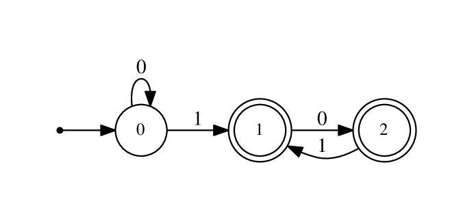
Figure 1: Fibonacci automaton for the set $S=\{1,2,4,7,12,\ldots\}$

Here the initial state is denoted by headless arrow entering, and the accepting states are denoted by double circles. To use this automaton, express $n$ in Fibonacci representation, start at the initial state labeled $0$, and follow the arrows according to the bits of $(n)_{F}$. If the automaton ends up in an accepting state, then $n\in S$. If at some point there is no possible move, or if the automaton ends in a non-accepting state, then $n\not\in S$.

4 Wythoff sequences

The values of the lower and upper Wythoff sequences have distinctive Fibonacci representations that were determined by Silber [16]:

Theorem 1.

• $n$ belongs to the lower Wythoff sequence iff $(n-1)_{F}$ ends in $0$;

• $n$ belongs to the upper Wythoff sequence iff $(n-1)_{F}$ ends in $01$.

For the purpose of this theorem, we pretend that every Fibonacci representation is preceded by at least one $0$.

It follows from this (we will see exactly how below) that there is a very simple Fibonacci automaton for the set of lower Wythoff numbers, and another for the set of upper Wythoff numbers. We give them below. Kawsumarng et al. [9] called these sets $B(\alpha)$ and $B(\alpha^{2})$, respectively, but we shall call them $L$ and $U$ (for lower and upper).

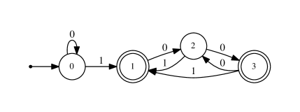
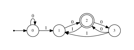
Figure 2: Fibonacci automata for the sets $L$ (left) and $U$ (right)

Similarly, Kawsumarng et al. defined $B_{0}(\alpha)=B_{(}\alpha)\cup\{0\}$ and $B_{0}(\alpha^{2})=B(\alpha^{2})\cup\{0\}$, but we will call these $L_{0}$ and $U_{0}$, respectively.

Recall that if $S,T\subseteq\mathbb{N}$, then $S+T$ denotes the sumset $\{s+t\,:\,s\in S,\ t\in T\}$. Now that we have automata for $L$ and $U$, we can find automata for their sumsets, using the following theorem [12]:

Theorem 2.

Given a first-order formula $F$ involving a Fibonacci-automatic set (or sets), addition, comparison, logical operators, and the universal and existential quantifiers, there is an automaton accepting the Fibonacci representations of those settings of the free variables that make $F$ true.

Not only does such an automaton exist; there is also an algorithm to produce it. This algorithm has been implemented in the free software called Walnut and written by Hamoon Mousavi [11].

For example, if we wish to compute the Fibonacci automaton for the sumset $L+U$, we only need to write the first-order formula

$$\phi:\exists a,b\ (n=a+b)\ \wedge\ a\in L\ \wedge\ b\in U,$$

translate it into Walnut’s syntax,

def lplusu "?msd_fib E a,b (n=a+b) & $lower(a) & $upper(b)":

and have Walnut compute the corresponding automaton recognizing the language

$$L(\phi)=\{(n)_{F}\,:\,\phi\text{ holds }\}.$$

Walnut’s syntax is more or less self-explanatory; we note that in Walnut, the symbol E represents the existential quantifier and the cryptic notation ?msd_fib indicates that we want to evaluate the predicate using the Fibonacci representation of integers. Here

• lower is Walnut’s name for $L:=B(\alpha)$;

• lower0 is Walnut’s name for $L_{0}:=B_{0}(\alpha)=B(\alpha)\cup\{0\}$;

• upper is Walnut’s name for $U:=B(\alpha^{2})$;

• upper0 is Walnut’s name for $U_{0}:=B_{0}(\alpha^{2})=B(\alpha^{2})\cup\{0\}$.

5 Finding automata for the sets $L,U,L_{0},U_{0}$

As we have seen, $n\in L$ iff $(n-1)_{F}$ ends in $0$, and $n\in U$ iff $(n-1)_{F}$ ends in $01$. The easiest way to specify these requirements is with a regular expression [8]. In Walnut we do this as follows:

reg end0 msd_fib "(0|1)*0":
reg end01 msd_fib "1|((0|1)*01)":

The alert reader will notice that we have allowed an arbitrary number of leading zeros at the beginning of our specifications. This is needed in Walnut for technical reasons. The straight bar $|$ represents logical “or”.

Now we can easily create Walnut predicates that assert that the Fibonacci representation of $n-1$ matches the given expressions.

def lower "?msd_fib Em $end0(m) & n=m+1":
def lower0 "?msd_fib $lower(n) | (n=0)":
def upper "?msd_fib Em $end01(m) & n=m+1":
def upper0 "?msd_fib $upper(n) | (n=0)":

When we run Walnut on these predicates, we get the automata given in Figure 2, as well as two automata for $L_{0}$ and $U_{0}$ (not depicted).

6 Theorem 3.1 of Kawsumarng et al.

We can now prove Theorem 3.1 of Kawsumarng et al., namely:

Theorem 3.

1. $L+L=\mathbb{N}-\{0,1,3\}$;

2. $L_{0}+L=\mathbb{N}-\{0\}$.

(The slight difference in notation between their paper and ours is because we use $\mathbb{N}=\{0,1,2,\ldots\}$, while Kawsumarng et al. used $\mathbb{N}=\{1,2,3,\ldots\}$.)

Proof.

We use the Walnut commands

def thm31i "?msd_fib ~Ea,b (n=a+b) & $lower(a) & $lower(b)":
def thm31ii "?msd_fib ~Ea,b (n=a+b) & $lower0(a) & $lower(b)":

which compute automata for the complements $\mathbb{N}-(L+L)$ and $\mathbb{N}-(L_{0}+L)$. These commands produce the automata depicted below.

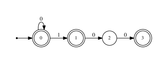
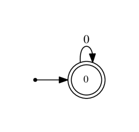
Figure 3: Automata for $\mathbb{N}-(L+L)$ (left) and $\mathbb{N}-(L_{0}+L)$ (right)

∎

Remark 4.

We point out that here the theorem-proving software Walnut is not just confirming something that could be conjecture from numerical evidence; rather, inspection of the automata produced here actually produces the statement of the theorem itself. So similar theorems can be churned out almost without human intervention, as we will see below.

7 Theorem 3.5 of Kawsumarng et al.

Now we are ready to prove Theorem 3.5 of Kawsumarng et al., namely:

Theorem 5.

1. $L+U=\mathbb{N}-\{F_{n}-1\,:\,n\geq 1\}$;

2. $L_{0}+U=\mathbb{N}-\{F_{n}-1\,:\,n\geq 1\text{ and }n\text{ odd }\}$;

3. $L+U_{0}=\mathbb{N}-\{F_{n}-1\,:\,n\geq 1\text{ and }n\text{ even }\}$.

Proof.

We use the Walnut commands

def thm35i "?msd_fib ~Ea,b (n=a+b) & $lower(a) & $upper(b)":
def thm35ii "?msd_fib ~Ea,b (n=a+b) & $lower0(a) & $upper(b)":
def thm35iii "?msd_fib ~Ea,b (n=a+b) & $lower(a) & $upper0(b)":

which compute automata for the complements $\mathbb{N}-(L+U)$, $\mathbb{N}-(L_{0}+U)$, and $\mathbb{N}-(L+U_{0})$. These commands produce the automata depicted below. By comparison with Figure 1, Kawsumarng et al.’s Theorem 3.5 immediately follows.

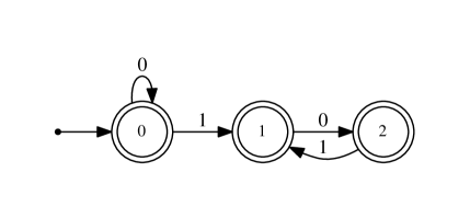
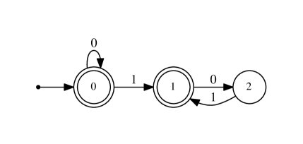
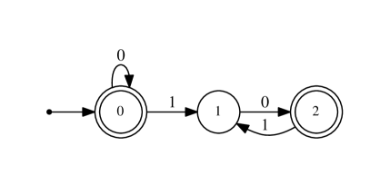
Figure 4: Automata for $\mathbb{N}-(L+U)$, $\mathbb{N}-(L_{0}+U)$, and $\mathbb{N}-(L+U_{0})$

∎

8 Theorem 3.7 of Kawsumarng et al.

We now move on to Theorem 3.7 of Kawsumarng et al.:

Theorem 6.

1. $L+U+U=\mathbb{N}-\{0,1,2,3,4,6,9\}$;

2. $L_{0}+U+U=\mathbb{N}-\{0,1,2,3,6\}$;

3. $L+U+U_{0}=\mathbb{N}-\{0,1,2,4\}$;

4. $L+U_{0}+U_{0}=\mathbb{N}-\{0,2\}$.

Proof.

As above, we can easily create Walnut predicates for the complements of the three sumsets:

def thm37i "?msd_fib ~Ea,b,c (n=a+b+c) & $lower(a) & $upper(b) & $upper(c)":
def thm37ii "?msd_fib ~Ea,b,c (n=a+b+c) & $lower0(a) & $upper(b) & $upper(c)":
def thm37iii "?msd_fib ~Ea,b,c (n=a+b+c) & $lower(a) & $upper(b) & $upper0(c)":
def thm37iv "?msd_fib ~Ea,b,c (n=a+b+c) & $lower(a) & $upper0(b) & $upper0(c)":

When we run these, we get the automata depicted below in Figure 5. Since each of these automata accept only a finite set, it is trivial to verify the claims.

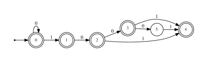
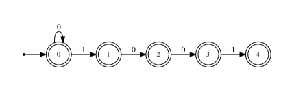
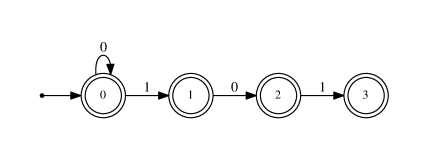
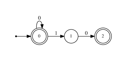
Figure 5: Automata for parts (i)-(iv) of Theorem 6

∎

9 Kawsumarng et al.’s Theorem 3.8

Theorem 7.

1. $U+U+U=\mathbb{N}-\{0,1,2,3,4,5,7,8,10,13,18,26\}$;

2. $U_{0}+U+U=\mathbb{N}-\{0,1,2,3,5,8,13\}$;

3. $U_{0}+U_{0}+U=\mathbb{N}-\{0,1,3,8\}$.

Proof.

As above, we can easily create Walnut predicates for the complements of the three sumsets:

def thm38i "?msd_fib ~Ea,b,c (n=a+b+c) & $upper(a) & $upper(b) & $upper(c)":
def thm38ii "?msd_fib ~Ea,b,c (n=a+b+c) & $upper0(a) & $upper(b) & $upper(c)":
def thm38iii "?msd_fib ~Ea,b,c (n=a+b+c) & $upper0(a) & $upper0(b) & $upper(c)":

When evaluated in Walnut these give the automata below in Figure 6. Since each of these automata accept only a finite set, it is trivial to verify the claims.

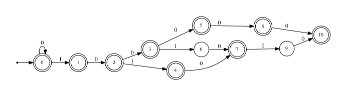
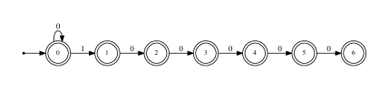
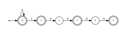
Figure 6: Automata for parts (i)-(iii) of Theorem 7

∎

10 The sumset $U+U$

Finally, perhaps the most interesting and complicated object in the paper of Kawsumarng et al. is the sumset $U+U$. They do not actually provide a clean explicit definition of this sumset, but with the method described here we can completely describe it with an automaton with 12 states, as follows:

Theorem 8.

The sumset $U+U$ is accepted by the automaton in Figure 7.

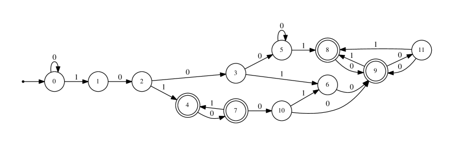
Figure 7: Automaton for the sumset $U+U$

Proof.

We use the Walnut command:

def uplusu "?msd_fib Ea,b (n=a+b) & $upper(a) & $upper(b)":

∎

With only a small amount of more work, from this automaton all of the results in Kawsumarng et al.’s Theorem 3.10 can be obtained. We omit the details, as they are just like what we have already done.

The facts that this automaton has 12 states and the sumset has an infinite complement explains why it is hard to write down a concise expression for $U+U$. We argue that the automaton is the best way to understand it. Furthermore, the automaton also explains their remarks about the “fractal” properties of $U+U$, since automatic sets are well-known to exhibit this kind of self-similarity [1].

11 New results on the Wythoff sets

11.1 Counting representable numbers

As an example of the power of the method, let’s look at a problem that Kawsumarng et al. did not study: how many numbers $<n$ are in the sumset $U+U$? Call this number $c(n)$.

We can easily create a Fibonacci automaton that recognizes the pairs $(m,n)$ such that $m<n$ and $m\in U+U$. From this, the techniques described in [6] explain how to explicitly compute a so-called “linear representation” for $c(n)$. It can be computed by the Walnut command below:

eval count2upp n "?msd_fib (m < n) & E a,b (m=a+b) & $upper(a) & $upper(b)":

In this case, the linear representation of rank $t$ that is produced is a triple $(v,\mu,w)$, where

• $v$ is a $1\times t$ matrix;

• $\mu$ is a morphism from $\{0,1\}$ to the set of $t\times t$ matrices with non-negative integer entries;

• $w$ is a $t\times 1$ matrix,

such that $c(n)=v\mu((n)_{F})w$. In this case, the rank is $33$; since it is so large, we do not display it here. However, it provides an efficient way to compute $c(n)$.

Furthermore, we can use it to explicitly compute $c(F_{n})$:

Theorem 9.

The number of elements of $U+U$ less than $F_{n}$ is $c(F_{n})$ and equals $2F_{n-2}+2-n$ for $n\geq 4$.

Proof.

We have $(F_{n})_{F}=10^{n-2}$ for $n\geq 2$. Therefore $c(F_{n})=v\mu(1)\mu(0)^{n-2}w$ for $n\geq 2$. If $M$ is a matrix, then it is well-known that each entry of $M^{i}$ satisfies a linear recurrence that is annihilated by the minimal polynomial of $M$. Of course, the same thing is also true for any linear combination of the entries of $M^{i}$. In this case, a symbolic algebra system such as Maple can easily compute the minimal polynomial of $M=\mu(0)$; it is $X^{3}(X+1)(X^{2}-X-1)(X-1)^{2}$. Now the fundamental theorem of linear recurrences tells us that $c(n)$ for $n\geq 5$ can be written as

$$c_{1}(-1)^{n}+c_{2}\alpha^{n}+c_{3}\beta^{n}+c_{4}n^{2}+c_{5}n+c_{6}$$

for some constants $c_{1},c_{2},\ldots,c_{6}$. We can then determine the constants by evaluating $c(n)$ for $5\leq n\leq 10$ and solving the resulting linear system. When we do this, and simplify, we get the desired result for $n\geq 5$. We can then check that the formula also holds for $n=4$. ∎

11.2 Number of representations

Given that a number is representable, how many different representations are there for $n$ as a sum of the form $a_{i}+a_{j}$, or $b_{i}+b_{j}$, or $a_{i}+b_{j}$? We can handle this problem using the enumeration capabilities of Walnut, as we did in the previous section. We can compute the corresponding linear representations using the commands below.

eval lowpluslow n "?msd_fib Eb (n=a+b) & $lower(a) & $lower(b)":
eval lowplusupp n "?msd_fib Eb (n=a+b) & $lower(a) & $upper(b)":
eval uppplusupp n "?msd_fib Eb (n=a+b) & $upper(a) & $upper(b)":

These give us linear representations of rank $19$, from which we can easily prove results like the following:

Theorem 10.

The number of pairs $(i,j)$ such that $F_{n}-1=a_{i}+a_{j}$ is $F_{n-1}-1$, for $n\geq 2$.

12 Generalization to higher-order recurrences

In their paper, Kawsumarng et al. ask about the generalization of sumsets to higher-order linear recurrences. One such linear recurrence is the famous Tribonacci sequence [7]. There is an analogue of the Fibonacci representation of integers, called the Tribonacci representation, and having many of the same properties. We denote it as $(n)_{T}$. Our automaton-based method also works for such sequences, and Tribonacci-automatic sequences are built into Walnut. For more examples of Walnut with the Tribonacci sequence, see [13].

Here the appropriate analogues of the sequences $(a_{n})_{n\geq 1}$ and $(b_{n})_{n\geq 1}$ we have considered so far in this paper are the Carlitz-Scoville-Hoggatt “sequences of higher order” $(A_{n})_{n\geq 1}$, $(B_{n})_{n\geq 1}$, and $(C_{n})_{n\geq 1}$; see [3, 4].

To give some idea of what kinds of things can be proved, consider the following two theorems:

Theorem 11.

A number $n$ cannot be written in the form $A(i)+B(j)$ iff $n=6$ or $(n)_{T}$ is a nonempty prefix of $100100100\cdots$.

Theorem 12.

Every integer $n$, except $0,1,2,3,4,5,6,8,10,12,19$, can be written in the form $n=A(i)+B(j)+C(k)$.

These, and many others, can be easily proved with Walnut almost immediately by mimicking the analysis we used above. We give the Walnut commands for these two theorems, and leave further exploration as a fun exercise for the reader.

reg tend0 msd_trib "(0|1)*0":
reg tend01 msd_trib "1|((0|1)*01)":
reg tend011 msd_trib "11|((0|1)*011)":
def aa "?msd_trib Em $tend0(m) & n=m+1":
def bb "?msd_trib Em $tend01(m) & n=m+1":
def cc "?msd_trib Em $tend011(m) & n=m+1":
def aaplusbb "?msd_trib ~Ea,b (n=a+b) & $aa(a) & $bb(b)":
def aaplusbbpluscc "?msd_trib ~Ea,b,c (n=a+b+c) & $aa(a) & $bb(b) & $cc(c)":

13 Remarks

The point we have tried to make by writing this paper is not to denigrate the ingenuity or hard work of others. It is, instead, to publicize the fact that many case-based arguments in combinatorics on words in the literature can now be replaced by some simple computations, using a decision procedure for the appropriate logical theory, using freely available software.

The advantages to this approach are many:

• long ad hoc arguments can be handled in a simple and unified way;

• drudgery is replaced by a software tool;

• the software allows us to conduct experiments with ease, giving us a “telescope” to view results that at first appear only distantly provable;

• in many cases Walnut’s results actually provide the complete statement of the desired result;

• the formalism of finite automata allow complicated results to be stated relatively simply;

• when the automata are very complicated, likely there is no really simple way to characterize the corresponding sets;

• much more general results, such as enumeration, can also be obtained; and finally,

• generalizations to other settings, such as the Tribonacci numbers here, are often easy and routine.

In this respect, the method described in this paper can be viewed as another weapon in the combinatorialist’s arsenal, much like the Wilf-Zeilberger method can be used for binomial coefficient identities and beyond [14]. We hope other authors will consider this approach in their work.

The free software Walnut we have discussed is available at

https://github.com/hamousavi/Walnut

and a manual for its use is [11]. The web page

https://cs.uwaterloo.ca/~shallit/walnut.html

on the author’s home page contains references to many papers using the approach we have described here.

References

- [1] A. Barbé and F. von Haeseler. Limit sets of automatic sequences. Adv. in Math. 175 (2003), 169–196.
- [2] Jason Bell, Thomas Finn Lidbetter, and Jeffrey Shallit. Additive number theory via approximation by regular languages, In M. Hoshi and S. Seki, eds., DLT 2018, Lect. Notes in Computer Science, Vol. 11088, Springer, 2018, pp. 121–132.
- [3] L. Carlitz, R. Scoville and V. E. Hoggatt, Jr. Fibonacci representations of higher order, Fib. Quart. 10 (1972), 43-69.
- [4] F. Michel Dekking, Jeffrey Shallit, and N. J. A. Sloane. Queens in exile: non-attacking queens on infinite chess boards. Electronic J. Combin. 27 (1) (2020), #P1.52.
- [5] C. F. Du, H. Mousavi, E. Rowland, L. Schaeffer, and J. Shallit. Decision algorithms for Fibonacci-automatic words, II: Related sequences and avoidability. Theoret. Comput. Sci. 657 (2017), 146–162.
- [6] Chen Fei Du, Hamoon Mousavi, Luke Schaeffer, and Jeffrey Shallit. Decision algorithms for Fibonacci-automatic words, III: Enumeration and abelian properties. Int. J. Found. Comput. Sci. 29 (8) (2016), 943–963.
- [7] M. Feinberg. Fibonacci-Tribonacci. Fib. Quart. 1 (3) (1963), 71–74.
- [8] John E. Hopcroft and Jeffrey D. Ullman, Introduction to Automata Theory, Languages, and Computation, Addison-Wesley, 1979.
- [9] S. Kawsumarng, T. Khemaratchatakumthorn, P. Noppakaew, and P. Pongsriiam. Sumsets associated with Wythoff sequences and Fibonacci numbers. Period. Math. Hung. (2020). https://doi.org/10.1007/s10998-020-00343-0.
- [10] C. G. Lekkerkerker. Voorstelling van natuurlijke getallen door een som van getallen van Fibonacci. Simon Stevin 29 (1952), 190–195.
- [11] H. Mousavi. Automatic theorem proving in Walnut. Available at http://arxiv.org/abs/1603.06017, 2016.
- [12] H. Mousavi, L. Schaeffer, and J. Shallit. Decision agorithms for Fibonacci-automatic words, I: Basic results. RAIRO Inform. Théor. App. 50 (2016), 39–66.
- [13] H. Mousavi and J. Shallit. Mechanical proofs of properties of the Tribonacci word. In F. Manea and D. Nowotka, eds., WORDS 2015, Lect. Notes in Comput. Sci., Vol. 9304, Springer, 2015, pp. 1–21.
- [14] Marko Petkovšek, Herbert S. Wilf, and Doron Zeilberger. . A. K. Peters, 1996.
- [15] Aayush Rajasekaran, Jeffrey Shallit, and Tim Smith. Additive number theory via automata theory. Theor. Comput. Systems 64 (2020), 542–567.
- [16] R. Silber. A Fibonacci property of Wythoff pairs. Fib. Quart. 14 (1972), 380–384.
- [17] N. J. A. Sloane et al. The On-Line Encyclopedia of Integer Sequences. Available at https://oeis.org, 2020.
- [18] E. Zeckendorf. Représentation des nombres naturels par une somme de nombres de Fibonacci ou de nombres de Lucas. Bull. Soc. Roy. Liège 41 (1972), 179–182.