MasterTwo: A Mathematica Package for the Automated Calculation of
Two Loop Diagrams in the Standard Model and Beyond

Abstract

The calculation of rare loop decays in the Standard Model of Particle Physics and its extensions is an extremely tedious work. The MATHEMATICA  package MasterTwo facilitates this task. It automatically calculates all loop integrals reducible to scalar integrals depending on up to two different masses independent of external momenta. MasterTwo consists of two sub packages, Fermions  and Integrals. Whereas Fermions covers the standard Dirac Algebra, Integrals performs the Taylor expansion, partial fraction, tensor reduction and the integration of the thus achieved scalar integrals. The package works completely inside MATHEMATICAand can be easily customised for both educational and research purposes.

,

Package summary
Manuscript Title: MasterTwo: A Mathematica Package for the Automated Calculation of
Two Loop Diagrams in the Standard Model and Beyond
Authors: S.Schilling
Package Title: MasterTwo
Version: 1.0
Journal Reference:
Catalogue identifier:
Licensing provisions: None
Programming language: MATHEMATICA
Computer: Computers running MATHEMATICA
Operating system: Linux, MacOs, Windows
RAM: Depending on the complexity of the problems
Keywords: two loop integration, heavy mass expansion, recurrence relations, tensor reduction, Dirac algebra, computer algebra, MATHEMATICA, B decays
PACS: 13.25.Hw, 14.80.Cp, 02.70.Wz
Classification: Computer Algebra
Nature of the physical problem: One- and two-loop integrals reducible to scalar integrals independent of external momenta and dependent on up to two different masses.
Solution method: Heavy Mass Expansion and recurrence relations to transform tensor integrals to a larger number of scalar master integrals. Loop integration of the thus obtained scalar master integrals.
Running time: Strongly depending on the problem and nature of diagram being calculated

1 Introduction

The calculation of rare (loop) decays in the Standard Model of Particle Physics (SM) is an extremely complex, error prone task, which should be (semi) automated with the help of computer algebra programs. The MATHEMATICA package MasterTwo was originally designed to facilitate such calculations arising in one and two-loop B-decays like $b\to s\;\gamma$ and $b\to sl^{+}l^{-}$ in the Standard Model of particle physics and and Two-Higgs-Doublet model extensions [1].
MasterTwo allows the automated calculation of all one- and two-loop integrals reducible to scalar integrals independent of external momenta and only dependent on up to two different masses. To do so it uses both the Heavy Mass Expansion [2] and recurrence relations [3] to transform tensor integrals to a larger number of scalar master integrals, which are then automatically integrated. The package’s lean structure should make it an ideal candidate for both research and educational purposes. MasterTwo consists of two sub packages, Fermions  and Integrals. Fermions  contains all routines regarding the Dirac Algebra, Integrals  summarises all routines concerning the tensor reduction, partial fraction of one and two-loop integrals and the subsequent integration of the thus arising scalar integrals. This manual is organized as follows: The physics background and mathematical methods involved are summarized in sections 2(package Fermions) and 3 (package Integrals), whereas sections 4 and 5 document the corresponding MATHEMATICA commands. Section 6 documents the installation of the package on the different operating systems Linux, Mac and Windows, whereas section 7 shows how the Standard Model output generated by the package FeynArts can be adapted for the further usage in MasterTwo. Finally we demonstrate the usage of MasterTwo on an example diagram of the two-loop decay $b\to s\;\gamma$ in section 8.

2 Fermions

Fermions can simplify Dirac expressions in $D$ dimensions  with an anticommuting $\gamma_{5}$. It provides the tools for standard operations like contracting indices, sorting expressions and the use of the Dirac equation. To calculate physical quantities as cross sections and decay-rates it allows furthermore to conjugate and square Dirac expressions and to compute traces over products of $\gamma$ matrices (for details see section 4.3).

2.1 Declarations and Constants

Before usage of the package, all arising masses, momenta, indices and polarisation vectors must first be declared. The documentation of the corresponding commands is given in 4.1.

There are a few constants predefined in Fermions:

• d denotes the space-time dimension.

• eps stands for $\epsilon$.

• L and R are the left- and the right-projectors, respectively: $\texttt{L}=1/2\;(1-\gamma_{5})$ and $\texttt{R}=1/2\;(1+\gamma_{5})$.

• Gamma5 stands for $\gamma_{5}$.

• Unit denotes the unit matrix.

• Sigma[mu,nu] is the tensor $\sigma_{\mu\nu}=i/2[\gamma_{\mu},\gamma_{\nu}]$.

The symbols L, R and Gamma5 are treated as projectors and, provided the expression is simple enough, are shifted to the left automatically in order to reduce the number of different terms. An expression like $\gamma_{\mu}L+R\gamma_{\mu}$ will therefore automatically be transformed into $2R\gamma_{\mu}$.

2.2 Notation and Syntax

After all the necessary declarations have been established, the corresponding symbols can be used inside Dirac expressions and alike.

Gamma matrices, tensors and projectors like $\gamma_{\mu},\;\sigma_{\mu\nu},\mathtt{L},\mathtt{R}$ and L and R matrices are given as expressions with the head Dirac, whereas scalar products are input as the function Scal. A few examples of simple structures:

$g_{\mu\nu}$	Scal[mu,nu],
$p_{\mu}$	Scal[p,mu],
$p\cdot q$	Scal[p,q],
1	Dirac[] (unit matrix in Dirac space),
$\gamma_{\mu}$	Dirac[mu],
$\not{p}$	Dirac[p],
$\gamma_{5}$	Dirac[Gamma5] and similar for $L$ and $R$,
$\sigma_{\mu\nu}$	Dirac[Sigma[mu,nu]].

Some more complicated structures involving products of $\gamma$ matrices and four-vectors might read:

$L\gamma_{\mu}\gamma_{\nu}\not{p}$	Dirac[L, mu, nu, p],
$p_{\mu}\gamma^{\mu}$	Scal[p, mu] Dirac[mu],
$\gamma_{\mu}(\not{p}+m_{b})\not{q}$	Dirac[mu, p + mb, q],
$R(m_{b}\gamma_{\mu}+p_{\mu})\gamma_{\nu}$	Dirac[R, mb mu + Unit Scal[p, mu], nu].

Note that masses inside Dirac structures need not to be provided with an extra Unit matrix, whereas this is indispensable for other structures like scalar products.

Fermions makes no difference between covariant (up) and contravariant (down) indices. It simply assumes that - if the same index appears twice - one is upper and the other lower and, if requested, takes the sum over them.

2.3 Dirac Algebra and Naive Dimensional Regularisation

The D-dimensional metric tensor $g$ is introduced satisfying

$$g_{\mu\nu}g^{\nu\mu}=g_{\mu}^{\mu}=D,$$ (1)

where $D=4-2\epsilon$ in all kind of expressions containing Lorentz indices. The Dirac gamma matrices $\gamma^{\mu}=(\gamma^{0},\gamma^{i})$, where the Latin index $i$ is employed to denote spatial indices 1,2,3, satisfy the anticommutation relations

$$\{\gamma^{\mu},\gamma^{\nu}\}=2g^{\mu\nu} = 2g_{\mu\nu}.$$ (2)

The $\gamma_{5}$ is defined by

$$\gamma_{5}=\gamma^{5}=i\gamma^{0}\gamma^{1}\gamma^{2}\gamma^{3}$$ (3)

and anti-commutes with all $\gamma^{\mu}$:

$$\{\gamma^{5},\gamma^{\mu}\}=0.$$ (4)

It has been emphasised in the literature that this rule leads to algebraic inconsistencies [4, 5]. Indeed, the naive dimensional regularisation (NDR) is inconsistent with

$$Tr(\gamma^{\mu}\gamma^{\nu}\gamma^{\rho}\gamma^{\sigma}\gamma_{5})\neq 0$$ (5)

for dimensions of space-time $D=4-2\epsilon$, $\epsilon\neq 0$ . However the latter condition is often considered to be necessary for an acceptable regularisation, since at $D=4$ we must find

$$Tr(\gamma^{\mu}\gamma^{\nu}\gamma^{\rho}\gamma^{\sigma}\gamma_{5})=4\mathrm{i}\varepsilon^{\mu\nu\rho\sigma}\;.$$ (6)

Provided one can avoid the calculation of traces like eq. (6) containing $\gamma_{5}$ matrices, it has been demonstrated in many explicit calculations [6] that the NDR gives correct results consistent with schemes without the $\gamma_{5}$ problem. From eq. (3) we get for the projectors $R=(1+\gamma^{5})/2$ and $L=(1-\gamma^{5})/2$

$$\gamma^{0}R=L\gamma^{0},\;\gamma^{0}L=R\gamma^{0}.$$ (7)

The package does not need an explicit representation of the algebra, it can thus handle objects of the form $\gamma_{\mu}\gamma_{\nu}$ rather than e.g. $\gamma_{0}\gamma_{2}$. The function DiracAlgebra performs the standard Dirac algebra according to eqs. (1), (2), (4) and (7). Further functions of Fermions (conjugations, traces) are documented in section 4.

3 Integrals

Integrals performs all the steps necessary to transform the integrals into scalar master integrals of up to two different masses and independent of external momenta and their subsequent loop integration. A full list of all the available commands is given by the command IntegralsInfo[]. A detailed documentation of all the functions introduced below is given in section 5.

3.0.1 Additional Declarations

Some functions of Integrals require the distinction between small and heavy masses or loop momenta and external momenta. Thus for the proper function of these functions additional declarations have to be made. Details can be found in section 5.1.

3.0.2 Representatin of Propagators

The propagator structure of one-loop integrals like

$$\frac{1}{(q_{1}^{2}-m_{1}^{2})^{n_{1}}}$$ (8)

is written in the programme as

$$\mathtt{AD[\underbrace{\mathtt{den[q_{1},m_{1}],\ldots,den[q_{1},m_{1}]}}_{\rm{n_{1}\;times}}]}.$$ (9)

In analogy, the propagator structure of two-loop integrals

$$\frac{1}{(q_{1}^{2}-m_{1}^{2})^{n_{1}}(q_{2}^{2}-m_{2}^{2})^{n_{2}}((q_{1}+q_{2})^{2}-m_{3}^{2})^{n_{3}}}$$ (10)

is written as

$${\scriptstyle{\mathtt{AD[\underbrace{\scriptstyle\mathtt{den[q_{1},m_{1}],\ldots,den[q_{1},m_{1}]}}_{\rm{n_{1}\;times}},\underbrace{\scriptstyle\mathtt{den[q_{2},m_{2}],\ldots,den[q_{2},m_{2}]}}_{\rm{n_{2}\;times}},\underbrace{\scriptstyle\mathtt{den[q_{1}+q_{2},m_{3}],\ldots,den[q_{1}+q_{2},m_{3}]}}_{\rm{n_{3}\;times}}]}}}.$$ (11)

3.1 Colour Algebra

Integrals with outgoing gluons or quarks can lead to a quite complicated colour structures. The following relations can be derived in the fundamental representation of $SU(N)$ [7]:

$$f^{bac}\textbf{T}^{c}\textbf{T}^{b} =\frac{1}{2}\;i\;N\textbf{T}^{a},$$ (12)

$$\textbf{T}^{c}\textbf{T}^{d}f^{dba}f^{acb} =\textbf{T}^{c}\textbf{T}^{d}N\delta^{dc}$$

$$=\frac{N^{2}-1}{2N}N=\frac{N^{2}-1}{2},$$ (13)

$$\textbf{T}^{a}\textbf{T}^{e}f^{adc}f^{dek}f^{ckb} =\frac{N}{2}\textbf{T}^{a}\textbf{T}^{e}f^{abe}=-i\frac{N^{2}}{4}\textbf{T}^{b}.$$ (14)

The function Color applies eqs. (12-14) for the special case $N=3$. Note that structure constants $f^{abc}$ are represented in the programme as SUNF[a,b,c], whereas products of generators $\textbf{T}^{a}\textbf{T}^{b}$ are represented as SUNT[a,b].

3.2 From Tensor Integrals to Scalar Integrals

Integrals was originally designed to facilitate the calculation of Wilson coefficients of mass dimension six operators of effective Hamiltonians of the the rare decays $b\to s\;\gamma$ and $b\to sl^{+}l^{-}$ in the SM and Two-Higgs-Doublet models. In the corresponding integrals two heavy mass scales arise: the top-mass and the $W$-mass (SM) or the charged Higgs mass (THDM). A typical propagator structure is given by

$$I=\frac{1}{(q_{1}^{2}-m_{1}^{2})^{n_{1}}(q_{1}^{2}-m_{2}^{2})^{n_{2}}((q_{2}+k_{1})^{2}-m_{2}^{2})^{n_{3}}((q_{1}+q_{2}+k_{2})-m_{2}^{2})^{n_{4}}},$$ (15)

where $q_{1}$ and $q_{2}$ are the loop momenta, $k_{1}$ and $k_{1}$ the external momenta, $n_{j}\geq 0$ and $\sum_{j}n_{j}=6$. The exact calculation of two-loop graphs with two mass scales is technically very demanding. Thus at the moment exact results for diagrams with more than one mass scale do not exist beyond one-loop. Therefore the Heavy Mass Expansion (HME) [2], an asymptotic expansion in small momenta and masses, is used.

3.2.1 Heavy Mass Expansion

The basic idea of the Heavy Mass Expansion (HME) is to use the hierarchy of mass scales and momenta to reduce complicated two-loop calculations to simpler ones. The following assumptions are made:

1. All the masses of a given Feynman diagram $\Gamma$ can be divided into a set of large $\underline{M}=\{M_{1},M_{2},\ldots$} and small $\underline{m}=\{m_{1},m_{2},\ldots\}$ masses.

2. All external momenta $\underline{k}=\{k_{1},k_{2},\ldots\}$ are small compared to the scale of the large masses $\underline{M}$.

The ansatz is that the dimensionally regularised (unrenormalised) Feynman integral $F_{\Gamma}$ associated with the Feynman diagram $\Gamma$ can be written as

$$F_{\Gamma}\stackrel{{\scriptstyle\underline{M}\to\infty}}{{\sim}}\sum_{\gamma}F_{\Gamma/\gamma}\circ{\cal T}_{\underline{k}^{\gamma},\underline{m}^{\gamma}}F_{\gamma}(\underline{k}^{\gamma},\underline{m}^{\gamma},\underline{M}),$$ (16)

where the sum is performed over all subgraphs $\gamma$ of $\Gamma$ which fulfil the following two conditions simultaneously:

• $\gamma$ contains all lines with heavy masses ($\underline{M}$),

• $\gamma$ consists of connected components that are one-particle-irreducible with respect to the lines with small masses ($\underline{m}$).

The operator ${\cal T}$ performs a Taylor expansion in the variables $k_{i}^{2}/M_{j}^{2}$ and $m_{l}^{2}/M_{j}^{2}$, where $k_{i}$ belongs to $\underline{k}^{\gamma}$, the set of external momenta with respect to the subgraph $\gamma$. $m_{l}$ belongs to the set of light masses $\underline{m}^{\gamma}$ of $\gamma$. $M_{j}$ is the heavy mass of the propagator to which the light mass or the external momenta belong to.

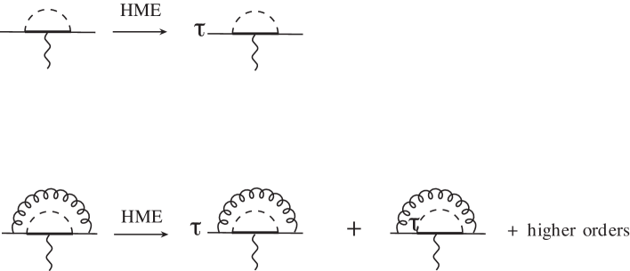
Figure 1: Expansion of the full theory in the HME for the example process $b\to s\;\gamma$. $\tau$ symbolises the Taylor expansion in small masses and momenta as described in eq. (16). Thick lines stand for heavy quarks (in this example the top mass), dashed lines heavy bosons like the $W^{\pm},\pi^{\pm}$ in the SM or the charged Higgs in the THDM. In line two we show the two subdiagrams needed to be evaluated in the HME.

After Taylor expansion of the two-loop integrals we need to deal with the calculation of a large number of rather simple integrals. Matching these results with effective low energy theories we find out to which mass power we must expand the Taylor series in the HME. In order to calculate Wilson coefficients of the rare b-decays $b\to s\;\gamma$ and $b\to sl^{+}l^{-}$ up to ${\cal O}(\alpha_{s})$-precision we have to match to an effective theory with operators of mass dimension six. Therefore it is sufficient to expand the integrands up to second order in external momenta and small masses. Expansion up to higher order in the external momenta would correspond to Wilson coefficients of operators of higher mass dimensions and can therefore be safely neglected. The Taylor expansion of the Feynman integrands in external momenta, as well as setting all the light masses to zero, creates spurious infrared divergences which can be regularised dimensionally. All these divergences cancel out in the matching conditions relating the full and the effective theory Green functions.

Taylor Expansion

The expansion in external momenta is performed by the function
TaylorExpansion. It performs the expansion of each propagator in external momenta up to ${\cal O}[($external momenta$)^{2}/M^{2}]$

$$\frac{1}{(q_{i}+k)^{2}-M^{2}}= \frac{1}{q_{i}^{2}-M^{2}}\left[1-\frac{k^{2}+2kq_{i}}{q_{i}^{2}-M^{2}}+\frac{4(kq_{i})^{2}}{(q_{i}^{2}-M^{2})^{2}}\right]+{\cal O}[k^{4}/M^{4}],$$ (17)

$$\frac{1}{(q_{1}+q_{2}+k)^{2}-M^{2}}= \frac{1}{(q_{1}+q_{2})^{2}-M^{2}}$$

$$\left[1-\frac{k^{2}+2kq_{1}+2kq_{2}}{(q_{1}+q_{2})^{2}-M^{2}}+\frac{4(kq_{1})^{2}+4(kq_{2})^{2}+8q_{1}kq_{2}}{((q_{1}+q_{2})^{2}-M^{2})^{2}}\right]$$

$$+{\cal O}[k^{4}/M^{4}],$$ (18)

where $q_{i}\;(i=1,2)$ are the loop momenta, $M$ is a heavy mass and $k$ an arbitrary external momentum.
The expansion in small masses up to second order

$$\frac{1}{q_{i}^{2}-m^{2}}=\frac{1}{q_{i}^{2}}\left[1+\frac{m^{2}}{q^{2}}\right]+{\cal O}[m^{4}/q^{4}],$$ (19)

where $m$ is a small mass, is performed by the function TaylorMass. The function expands automatically in all masses not declared as heavy masses with DeclareHeavyMass.

Scaling

The routine Scaling multiplies all light masses and external momenta with a factor $x$ and sets all terms $x^{n}$ with $n>2$ to zero. This is justified in the calculation of Wilson coefficients corresponding to operators of mass dimension six. Keeping terms with $n>2$ would correspond to the calculation of contributions to Wilson coefficients of higher mass dimensions.

3.2.2 Partial Fraction Decomposition and Simplification of Numerators

The routine PartialFractionOne (one-loop case) and PartialFractionTwo (two-loop case) apply partial fraction decompositions. The resulting integrals contain in the propagator denominator a single mass parameter together with a given loop momentum.

$$\frac{1}{(q^{2}-m_{1}^{2})(q^{2}-m_{2}^{2})} =\frac{1}{m_{1}^{2}-m_{2}^{2}}\left[\frac{1}{q^{2}-m_{1}^{2}}-\frac{1}{q^{2}-m^{2}}\right],$$ (20)

$$\frac{q^{2}}{(q^{2}-m_{1}^{2})(q^{2}-m_{2}^{2})} =\frac{1}{m_{1}^{2}-m_{2}^{2}}\left[\frac{m_{1}^{2}}{q^{2}-m_{1}^{2}}-\frac{m_{2}^{2}}{q^{2}-m_{2}^{2}}\right].$$ (21)

Furthermore the routines perform the following relations to get successively rid of loop momenta in the numerator:

$$\frac{(q_{i}^{2})^{n}}{q_{i}^{2}-m^{2}}= (q_{i}^{2})^{n-1}+\frac{(q_{i}^{2})^{n-1}m^{2}}{q_{i}^{2}-m^{2}}\;(i=1,2),$$ (22)

$$\frac{(q_{1}q_{2})^{n}}{(q_{1}^{2}-m_{1}^{2})(q_{2}^{2}-m_{2}^{2})((q_{1}+q_{2})^{2}-m_{3}^{2})}= \frac{1}{2}(q_{1}q_{2})^{n-1}\left[\frac{1}{(q_{1}^{2}-m_{1}^{2})(q_{2}^{2}-m_{2}^{2})}\right.$$

$$-\frac{1}{(q_{2}^{2}-m_{2}^{2})((q_{1}+q_{2})^{2}-m_{3}^{2})}$$

$$-\frac{1}{(q_{1}^{2}-m_{2}^{2})((q_{1}+q_{2})^{2}-m_{3}^{2})}$$

$$+\left.\frac{m_{3}^{2}-m_{1}^{2}-m_{2}^{2}}{(q_{1}^{2}-m_{1}^{2})(q_{2}^{2}-m_{2}^{2})((q_{1}+q_{2})^{2}-m_{3}^{2})}\right]$$ (23)

with $n\geq 1$. In a last step all vanishing massless integrals are set to zero [8]:

$$\int d^{D}q\frac{1}{q^{2}{}^{\alpha}}=0.$$ (24)

3.2.3 Tensor Reduction

The idea of the tensor reduction is to express tensor integrals in terms of scalar integrals. As integrals over an antisymmetric integrand with symmetric integration boundaries are zero, all integrands with an odd number of loop momenta $q_{i}^{\alpha},(i={1,2})$ in the nominator can be set to zero before performing the proper tensor reduction. The basic relations for the tensor reduction of one-loop integrals are given by

$$\int d^{D}q\;{q^{\alpha_{1}}q^{\alpha_{2}}}{A(q^{2})} =\frac{1}{D}\int d^{D}q^{2}g^{\alpha_{1}\alpha_{2}}A(q^{2}),$$ (25)

$$\int d^{D}q\;q^{\alpha_{1}}q^{\alpha_{2}}q^{\alpha_{3}}q^{\alpha_{4}}A(q^{2}) =\frac{1}{D^{2}+2D}$$

$$\int d^{D}q^{4}(g^{\alpha_{1}\alpha_{2}}g^{\alpha_{3}\alpha_{4}}+g^{\alpha_{1}\alpha_{3}}g^{\alpha_{2}\alpha_{4}}+g^{\alpha_{1}\alpha_{4}}g^{\alpha_{2}\alpha_{3}})A(q^{2}),$$ (26)

$$\int d^{D}q\;q^{\alpha_{1}}q^{\alpha_{2}}\dots q^{\alpha_{2k}}A(q^{2}) =\frac{\Gamma(2-\epsilon)}{2^{k}\Gamma(2-\epsilon+k)}\int d^{D}q^{2k}{\bf{X^{(k)}}}\;A(q^{2}),$$ (27)

where $A(q^{2})$ is an arbitrary scalar function depending on Lorentz invariants of the loop momentum $q$ and masses. Usually it is a product of powers of propagators

$$\frac{1}{(q^{2}-m^{2})^{n_{1}}}$$ (28)

times a polynomial of $q^{2}$. $\bf{X^{(k)}}$ stands for permutations of metric tensor components $g^{\alpha_{j}\alpha_{k}}$. The routine TensorOne performs the tensor reduction of one-loop integrals for up to nine Lorentz indices. Results are Taylor expanded in $\epsilon$ up to second order. The one-loop relations eqs.  (25-27) can be generalised to the case of two-loop integrals [9] [10]

$$\int d^{D}q_{1}d^{D}q_{2}\;\;{q_{1}^{\alpha_{1}}q_{2}^{\alpha_{2}}}{A(q_{1},q_{2})}= \frac{1}{D}\int d^{D}q_{1}d^{D}q_{2}\;A(q_{1},q_{2})\;(q_{1}\cdot q_{2}){g^{\alpha_{1}\alpha_{2}}},$$ (29)

$$\int d^{D}q_{1}d^{D}q_{2}\;\;A(q_{1},q_{2})q_{1}^{\alpha_{1}}q_{1}^{\alpha_{2}}q_{1}^{\alpha_{3}}q_{2}^{\alpha_{4}}= \frac{1}{D^{2}+2D}\int d^{D}q_{1}d^{D}q_{2}\;\;A(q_{1},q_{2})q_{1}^{2}\;(q_{1}\cdot q_{2})$$

$$(g^{\alpha_{1}\alpha_{2}}g^{\alpha_{3}\alpha_{4}}+g^{\alpha_{1}\alpha_{3}}g^{\alpha_{2}\alpha_{4}}+g^{\alpha_{1}\alpha_{4}}g^{\alpha_{2}\alpha_{3}})$$ (30)

$$\int d^{D}q_{1}d^{D}q_{2}\;A(q_{1},q_{2}){q_{1}^{\alpha}q_{1}^{\beta}q_{2}^{\gamma}q_{2}^{\delta}}= \frac{1}{D^{3}+D^{2}-2D}\int d^{D}q_{1}d^{D}q_{1}\;A(q_{1},q_{2})$$

$$\bigl{[}\left((1+D){q_{1}^{2}q_{2}^{2}}-2{(q_{1}\cdot q_{2})^{2}}\right)g^{\alpha_{1}\alpha_{2}}g^{\alpha_{3}\alpha_{4}}$$

$$+\left(-{q_{1}^{2}q_{2}^{2}+D}{(q_{1}\cdot q_{2})^{2}}\right)g^{\alpha_{1}\alpha_{3}}g^{\alpha_{2}\alpha_{4}}$$

$$+g^{\alpha_{1}\alpha_{4}}g^{\alpha_{2}\alpha_{3}})\bigr{]},$$ (31)

where $A(q_{1},q_{2})$ is an arbitrary scalar function of $q_{1}$ and $q_{2}$ and arbitrary masses. It is usually a product of powers of propagators

$$\frac{1}{(q_{1}^{2}-m_{1}^{2})^{n_{1}}(q_{2}^{2}-m_{2}^{2})^{n_{2}}((q_{1}+q_{2})^{2}-m_{3}^{2})^{n_{3}}}$$ (32)

times a polynomial in $q_{1}^{2}$, $q_{1}^{2}$, $q_{1}q_{2}$, but the concrete form of this function has no importance for the tensor reduction. The function TensorTwo performs the two-dimensional tensor reduction for up to four Lorentz indices. In the case of factorising integrals corresponding to $c=0$ in the integrand of eq. (32), TensorTwo performs a one-dimensional tensor reduction calling TensorOne. From the tensor reduction we obtain additional terms of $q_{1}^{2},\;q_{2}^{2}$ or $q_{1}q_{2}$ in the numerator. This makes a subsequent usage of the identities PartialFractionOne and PartialFractionTwo, described in section 3.2.2, necessary.

3.2.4 Substitutions

The function Substitutions makes substitution in the integrands of factorising two-loop-integrals such that the propagator structure contains no overlapping loop momenta by applying the following relations

$$\int d^{D}q_{1}d^{D}q_{2}{\textstyle{\dfrac{S(q_{1},q_{2})}{(q_{1}^{2}-m_{1}^{2})^{n_{1}}((q_{1}+q_{2})^{2}-m_{2}^{2})^{n_{3}}}}} =\int d^{D}q_{1}d^{D}q_{2}\dfrac{S(q_{1},q_{2}-q_{1})}{(q_{1}^{2}-m_{1}^{2})^{n_{1}}(q_{2}^{2}-m_{2}^{2})^{n_{3}}},$$ (33)

$$\int d^{D}q_{1}d^{D}q_{2}\frac{S(q_{1},q_{2})}{(q_{2}^{2}-m_{1}^{2})^{n_{2}}((q_{1}+q_{2})^{2}-m_{2}^{2})^{n_{3}}} =\int d^{D}q_{1}d^{D}q_{2}\frac{S(q_{1}-q_{2},q_{2})}{(q_{2}^{2}-m_{1}^{2})^{n_{1}}(q_{1}^{2}-m_{2}^{2})^{n_{3}}},$$ (34)

where $S(q_{1},q_{2})$ is a polynomial in $q_{1}^{2}$, $q_{2}^{2}$ and $q_{1}\cdot q_{2}$. A subsequent final partial fraction of the so obtained integrands leads then to the desired scalar integrals.

3.2.5 Transforming the Propagator Structure

The routine SimplifyPropagator transforms the propagator structure of a scalar loop integrals to the forms needed for the loop integration functions. Thus the propagator structure of non-factorising scalar two-loop integrals eq. (11) is transformed to the short form

$$\mathtt{G[i[m_{1},n_{1}],i[m_{2},n_{2}],i[m_{3},n_{3}]]}.$$ (35)

The routine replaces the propagator structure of factorising two-lop integrals

$$\mathtt{AD[\underbrace{\mathtt{den[q_{1},m_{1}],....,den[q_{1},m_{1}]}}_{\rm{n_{1}\;times}},\underbrace{\mathtt{den[q_{2},m_{2}],....,den[q_{2},m_{2}]}}_{\rm{n_{2}\;times}}]}$$ (36)

with

$$\mathtt{AD[i[m_{1},n_{1}],i[m_{2},n_{2}]]}$$ (37)

and the propagator structure of one-loop integrals

$$\frac{1}{(q_{1}^{2}-m_{1}^{2})^{n_{1}}}$$ (38)

by

$${\mathtt{AD[i[m_{1},n_{1}]]}}.$$ (39)

SimplifyPropagator orders furthermore scalar two-loop integrals with one vanishing mass in the denominator in such a way that the propagator denominator with overlapping loop momenta has always no additional mass term ($m_{3}=0$):

$$\int d^{D}q_{1}d^{D}q_{2}\frac{1}{(q_{1}^{2})^{n_{3}}(q_{2}^{2}-m_{2}^{2})^{n_{2}}((q_{1}+q_{2})^{2}-m_{1}^{2})^{n_{1}}}$$

$$=\int d^{D}q_{1}d^{D}q_{2}\frac{1}{(q_{1}^{2}-m_{2}^{2})^{n_{2}}(q_{2}^{2})^{n_{3}}((q_{1}+q_{2})^{2}-m_{1}^{2})^{n_{1}}}$$

$$=\int d^{D}q_{1}d^{D}q_{2}\frac{1}{(q_{1}^{2}-m_{1}^{2})^{n_{1}}(q_{2}^{2}-m_{2}^{2})^{n_{2}}((q_{1}+q_{2})^{2})^{n_{3}}}.$$ (40)

The last line of eq. (40) is the ordering of propagator denominators needed for the following loop integration routines. This ordering is necessary, as the two-loop integrals are represented in the programme as a non-commuting list.

3.3 Loop Integration of Scalar One Loop Integrals

After Taylor expansion, tensor reduction and subsequent partial fractions the one-loop tensor integrals are transformed to a bigger number of scalar integrals proportional to [11]:

$$\mu^{2\epsilon}\int\frac{d^{D}\;q}{(2\pi)^{-2\epsilon}}\frac{1}{(q^{2}-m^{2})^{n}} =\frac{\mu^{2\epsilon}}{(2\pi)^{-2\epsilon}}\frac{\pi^{D/2}\;\Gamma(1+\epsilon)}{(m^{2})^{n-D/2}}\;C^{(1)}_{n}$$

$$=\frac{\pi^{2}}{(m^{2})^{n-2}}\;\left(\left(\frac{\mu^{2}}{m^{2}}\right)^{\epsilon}\;2^{2\epsilon}\pi^{\epsilon}\;\Gamma(1+\epsilon)\right)\;C^{(1)}_{n}$$

$$=\frac{\pi^{2}}{(m^{2})^{n-2}}N_{\epsilon}^{(1)}(m)\;C^{(1)}_{n},$$ (41)

where for arbitrary $n$ and $m$ [12]:

$$N_{\epsilon}^{(1)}(m) =\left(\frac{\mu^{2}}{m^{2}}\right)^{\epsilon}2^{2\epsilon}\pi^{\epsilon}\;\Gamma(1+\epsilon)$$

$$=1-\epsilon\kappa+\epsilon^{2}\left(\frac{1}{12}\pi^{2}+\frac{1}{2}\kappa(m)^{2}\right)+{\cal{O}}(\epsilon)^{3},$$ (42)

$$\kappa(m) =\gamma_{E}-\ln(4\pi)+\ln\frac{m^{2}}{\mu^{2}},$$ (43)

$$C^{(1)}_{n} =i\frac{(-1)^{n}}{(n-1)!}(1+\epsilon)_{n-3},$$ (44)

which vanishes for $n\leq 0$. In eq. (44) we introduced the Pochhammer symbol

$$(a)_{k}=\frac{\Gamma(a+k)}{\Gamma(a)}=\left\{\begin{array}[]{cc}a(a+1)(a+2)...(a+k-1),&k\geq 1,\\ 1,&k=0,\\ 1/[(a-1)(a-2)...(a-|k|)],&k\leq-1\end{array}\right.$$ (45)

for integer $k$ and complex $a$. The prefactors of $C^{(1)}_{n}$ are chosen such that $C^{(1)}_{n}$ is free of common factors of the one-loop integration. The factor $N_{\epsilon}^{(1)}(m_{1})$ summarises the $\epsilon$-dependent part of the common prefactors. The function ScalIntOne performs the scalar one-loop integration by replacing the propagator structure AD[i[m,n]] by the right hand side of eq. (41):

$$\mathtt{AD[i[m,n]]}\rightarrow\ \frac{\pi^{2}}{(m^{2})^{n-2}}\mathtt{Ne[m]\;C^{(1)}_{n}},$$ (46)

where Ne[m] corresponds to eq. (3.3) and $\mathtt{C^{(1)}_{n}}$ to eq. (44) up to second order in eps. The final result is expanded in eps up to first order.

3.4 Loop Integration of Scalar Two Loop Integrals

3.4.1 Recurrence Relations

In this section we will show how to reduce scalar two loop integrals independent of external momenta to master integrals, where the highest power of all appearing propagators is one. These master integrals can then be automatically integrated.

We will first give a general derivation of the recurrence relations for arbitrary masses $m_{1},\;m_{2}$ and $m_{3}$ for the integral

$$G_{n_{1},n_{2},n_{3}}^{m_{1},m_{2},m_{3}} \equiv\frac{\mu^{4\epsilon}}{(2\pi)^{-4\epsilon}}\int d^{D}q_{1}d^{D}q_{2}\frac{1}{(q_{1}^{2}-m_{1}^{2})^{n_{1}}(q_{2}^{2}-m_{2}^{2})^{n_{2}}((q_{1}+q_{2})^{2}-m_{3}^{2})^{n_{3}}}.$$ (47)

Its propagator structure is written in the package as $\mathtt{G[i[m_{1},n_{1}],i[m_{2},n_{2}],i[m_{3},n_{3}]]}$. The derivation of the recurrence relations starts with the following identities [3]:

$$\int d^{D}q_{1}d^{D}q_{2}\frac{\partial}{\partial q_{1}^{\mu}}\left(\frac{q_{1}^{\mu}}{(q_{1}^{2}-m_{1}^{2})^{n_{1}}(q_{2}^{2}-m_{2}^{2})^{n_{2}}((q_{1}+q_{2})^{2}-m_{3}^{2})^{n_{3}}}\right) =0,$$ (48)

$$\int d^{D}q_{1}d^{D}q_{2}\frac{\partial}{\partial q_{2}^{\mu}}\left(\frac{q_{2}^{\mu}}{(q_{1}^{2}-m_{1}^{2})^{n_{1}}(q_{2}^{2}-m_{2}^{2})^{n_{2}}((q_{1}+q_{2})^{2})-m_{3}^{2})^{n_{3}}}\right) =0,$$ (49)

$$\int d^{D}q_{1}d^{D}q_{2}\frac{\partial}{\partial{q_{1}^{\mu}}}\left(\frac{q_{1}^{\mu}}{(q_{1}^{2}-m_{1}^{2})^{n_{1}}((q_{1}+q_{2})^{2}-m_{2}^{2})^{n_{2}}(q_{2}^{2}-m_{3}^{2})^{n_{3}}}\right) =0.$$ (50)

Substitutions of the integration variables in eq. (48) lead to eqs. ((49)-(50)). With the help of the the Gaussian integral theorem we can transform the integral to a vanishing surface integral with symmetric boundaries and an asymmetric integrand. In oder to simplify the notation we will use

$$G_{n_{1},n_{2},n_{3}}^{m_{1},m_{2},m_{3}}\equiv G_{n_{1},n_{2},n_{3}}$$ (51)

in this section. From eq. (48) we get

$$(D-2n_{1}-n_{3})G_{n_{1},n_{2},n_{3}}= 2n_{1}m_{1}^{2}G_{n_{1}+1,n_{2},n_{3}}+n_{3}(G_{n_{1}-1,n_{2},n_{3}+1}-G_{n_{1},n_{2}-1,n_{3}+1})$$

$$+n_{3}(m_{1}^{2}-m_{2}^{2}+m_{3}^{2})G_{n_{1},n_{2},n_{3}+1}.$$ (52)

From eq. (49) or directly by replacing $n_{1}\leftrightarrow n_{2}$ and $m_{1}\leftrightarrow m_{2}$ in eq. (3.4.1) we get

$$(D-2n_{2}-n_{3})G_{n_{1},n_{2},n_{3}}= 2n_{2}m_{2}^{2}G_{n_{1},n_{2}+1,n_{3}}+n_{3}(G_{n_{1},n_{2}-1,n_{3}+1}-G_{n_{1}-1,n_{2},n_{3}+1})$$

$$+n_{3}(m_{2}^{2}-m_{1}^{2}+m_{3}^{2})G_{n_{1},n_{2},n_{3}+1}.$$ (53)

From eq. (50) we obtain

$$(D-2n_{1}-n_{2})G_{n_{1},n_{2},n_{3}}= 2n_{1}m_{1}^{2}G_{n_{1}+1,n_{2},n_{3}}+n_{2}(G_{n_{1}-1,n_{2}+1,n_{3}}-G_{n_{1},n_{2}+1,n_{3}-1})$$

$$+n_{2}(m_{1}^{2}+m_{2}^{2}-m_{3}^{2})G_{n_{1},n_{2}+1,n_{3}}.$$ (54)

The last three equations connect integrals with the sum of powers $n_{1}+n_{2}+n_{3}$ with integrals where the sum of the powers is lowered by 1. They form an equation system, which can be used to extract the integrals
$G_{n_{1}+1,n_{2},n_{3}},\;G_{n_{1},n_{2}+1,n_{3}}\;G_{n_{1},n_{2},n_{3}+1}$. Solving it we obtain the following recurrence relations [3]:

$$G_{n_{1}+1,n_{2},n_{3}}= \frac{1}{n_{1}\;m_{1}^{2}\;\Delta(m_{1},m_{2},m_{3})}$$

$$\bigl{\{}\bigl{[}n_{2}\;(m_{1}^{2}-m_{3}^{2})(m_{1}^{2}-m_{2}^{2}+m_{3}^{2})+n_{3}\;(m_{1}^{2}-m_{2}^{2})(m_{1}^{2}+m_{2}^{2}-m_{3}^{2})$$

$$\left.+D\;m_{1}^{2}\;(-m_{1}^{2}+m_{2}^{2}+m_{3}^{2})-n_{1}\;\Delta\;(m_{1},m_{2},m_{3})\right]G_{n_{1},n_{2},n_{3}}$$

$$+n_{2}\;m_{2}^{3}(m_{1}^{2}-m_{2}^{2}+m_{3}^{2})\left[G_{n_{1},n_{2}+1,n_{3}-1}-G_{n_{1}-1,n_{2}+1,n_{3}}\right]$$

$$+n_{3}\;m_{3}^{2}(m_{1}^{2}+m_{2}^{2}-m_{3}^{2})[G_{n_{1},n_{2}-1,n_{3}+1}-G_{n_{1}-1,n_{2},n_{3}+1}]\bigr{\}}$$ (55)

with the determinant of the corresponding equation system

$$\Delta(m_{1},m_{2},m_{3})=2(m_{1}^{2}m_{2}^{2}+m_{1}^{2}m_{3}^{2}+m_{2}^{2}m_{3}^{2})-(m_{1}^{4}+m_{2}^{4}+m_{3}^{4}).$$ (56)

Replacing $n_{1}\leftrightarrow n_{2}$ and $m_{1}\leftrightarrow m_{2}$ in eq. (3.4.1) we get

$$G_{n_{1},n_{2}+1,n_{3}}= \frac{1}{n_{2}\;m_{2}^{2}\;\Delta(m_{1},m_{2},m_{3})}$$

$$\bigl{\{}\left[n_{1}\;(m_{2}^{2}-m_{3}^{2})(m_{2}^{2}-m_{1}^{2}+m_{3}^{2})+n_{3}\;(m_{2}^{2}-m_{1}^{2})(m_{1}^{2}+m_{2}^{2}-m_{3}^{2})\right.$$

$$\left.+D\;m_{2}^{2}\;(-m_{2}^{2}+m_{1}^{2}+m_{3}^{2})-n_{2}\;\Delta(m_{1},m_{2},m_{3})\right]G_{n_{1},n_{2},n_{3}}$$

$$+n_{1}\;m_{1}^{2}(m_{2}^{2}-m_{1}^{2}+m_{3}^{2})\left[G_{n_{1}+1,n_{2},n_{3}-1}-G_{n_{1}+1,n_{2}-1,n_{3}}\right]$$

$$+n_{3}\;m_{3}^{2}(m_{1}^{2}+m_{2}^{2}-m_{3}^{2})\left[G_{n_{1}-1,n_{2},n_{3}+1}-G_{n_{1},n_{2}-1,n_{3}+1}\right]\bigr{\}}.$$ (57)

In analogy, we get by replacing $n_{1}\leftrightarrow n_{3}$ and $m_{1}\leftrightarrow m_{3}$ in eq. (3.4.1)

$$G_{n_{1},n_{2},n_{3}+1}= \frac{1}{n_{3}\;m_{3}^{2}\;\Delta(m_{1},m_{2},m_{3})}$$

$$\bigl{\{}\left[n_{1}(m_{3}^{2}-m_{2})^{2})(m_{2}^{2}-m_{1}^{2}+m_{3}^{2})+n_{2}(m_{3}^{2}-m_{1}^{2})(m_{1}^{2}+m_{3}^{2}-m_{2}^{2})\right.$$

$$\left.+D\;m_{3}^{2}(-m_{3}^{2}+m_{1}^{2}+m_{2}^{2})-n_{3}\;\Delta(m_{1},m_{2},m_{3})\right]G_{n_{1},n_{2},n_{3}}$$

$$+n_{1}\;m_{1}^{2}(m_{2}^{2}-m_{1}^{2}+m_{3}^{2})\left[G_{n_{1}+1,n_{2}-1,n_{3}}-G_{n_{1}+1,n_{2},n_{3}-1}\right]$$

$$+n_{2}\;m_{2}^{2}(m_{1}^{2}+m_{3}^{2}-m_{2}^{2})\left[G_{n_{1}-1,n_{2}+1,n_{3}}-G_{n_{1},n_{2}+1,n_{3}-1}\right]\bigr{\}}.$$ (58)

The general recurrence relations eqs (3.4.1), (3.4.1) and (3.4.1) are implemented in the rule recurrence which is part of the integration routine ScalIntTwoThreeMasses.

Recurrence Relations for Scalar Integrals with One Massless Propagator

In the following we consider the special case, that one of the masses in eq. (3.4.1) vanishes. Without restrictions we can choose this mass to be $m_{3}$. Taking the limit $m_{3}\rightarrow 0$ we get from eqs. (3.4.1) and (3.4.1)

$$\begin{array}[]{ccrlrl}G_{n_{1}+1,n_{2},n_{3}}^{m_{1},m_{2},0}&=&\frac{1}{m_{1}^{2}\;n_{1}(1-x)}&\lx@intercol\left\{[D-n_{1}-n_{2}-n_{3}+x(n_{1}-n_{3})]G_{n_{1}n_{2}n_{3}}^{m_{1},m_{2},0}\right.\hfil\lx@intercol\vspace{0.2cm}\\ &&&+&xn_{2}&\left.\left[G_{n_{1}-1,n_{2}+1,n_{3}}^{m_{1},m_{2},0}-G_{n_{1},n_{2}+1,n_{3}-1}^{m_{1},m_{2},0}\right]\right\},\end{array}$$ (59)

$$\begin{array}[]{ccrlrl}G_{n_{1},n_{2}+1,n_{3}}^{m_{1},m_{2},0}&=&-\frac{1}{m_{2}^{2}n_{2}x(1-x)}&\lx@intercol\left\{[x(D-n_{1}-n_{2}-n_{3})+n_{2}-n_{3}]G_{n_{1}n_{2}n_{3}}^{m_{1},m_{2},0}\right.\hfil\lx@intercol\vspace{0.2cm}\\ &&&+&n_{1}&\left.\left[G_{n_{1}+1,n_{2}-1,n_{3}}^{m_{1},m_{2},0}\right]\right\},\end{array}$$ (60)

where $x=m_{2}^{2}/m_{1}^{2}$ [3]. From eq. (3.4.1) we see that the limit $m_{3}\rightarrow 0$ does not exist for $G_{n_{1},n_{2},n_{3}+1}^{0}$. The recurrence relation for $G_{n_{1},n_{2},n_{3}+1}^{0}$ in this limit can be derived from eq. (3.4.1) by eliminating $G_{n_{1}+1,n_{2},n_{3}}^{0}$ with the help of eq. (3.4.1) and $G_{n_{1},n_{2}+1,n_{3}}^{0}$ with the help of eq. (3.4.1). Thus we obtain

$$\begin{array}[]{ccrlrl}G_{n_{1},n_{2},n_{3}+1}^{m_{1},m_{2},0}&=&\frac{1}{m_{1}^{2}n_{3}(1-x)^{2}}&\lx@intercol\left\{[(1+x)(-D)+2n_{2}+(1+3x)n_{3}]G_{n_{1}n_{2}n_{3}}^{m_{1},m_{2},0}\right.\hfil\lx@intercol\vspace{0.2cm}\\ &&&+&2xn_{2}&\left[G_{n_{1},n_{2}+1,n_{3}-1}^{m_{1},m_{2},0}-G_{(n_{1}-1)(n_{2}+1)n_{3}}^{m_{1},m_{2},0}\right]\vspace{0.2cm}\\ &&&+&(1-x)n_{3}&\left.\left[G_{n_{1}(n_{2}-1)(n_{3}+1)}^{m_{1},m_{2},0}-G_{(n_{1}-1)n_{2}(n_{3}+1)}^{m_{1},m_{2},0}\right]\right\}.\end{array}$$ (61)

Eqs. (59-61) are implemented in the rule recurrenceb. This rule is part of the integration routine ScalIntTwo.

3.4.2 Loop Integration of Master Integrals

In the last section we have shown how to reduce scalar two-loop integrals independent of external momenta to master integrals. This section will focus on the loop integration of special cases of these master integrals. We will focus on integrals with only two different masses ($m_{1}=m_{3}$) and the case of one vanishing mass ($m_{3}=0$) in eq. (47).

Scalar Two loop Integrals with Two Different Masses

The routine ScalIntTwoThreeMasses can automatically perform the integration of scalar two-loop integrals of the type of eq. (47) for the special case $m_{1}=m_{3}$. In a first step the integrands are ordered by making the following substitutions

$$\int\tfrac{d^{D}q_{1}d^{D}q_{2}}{(2\pi)^{-4\epsilon}}\tfrac{1}{(q_{1}^{2}-m_{1}^{2})^{n_{1}}(q_{2}^{2}-m_{1}^{2})^{n_{2}}((q_{1}-q_{2})^{2}-m_{2}^{2})^{n_{3}}}$$

$$= \int\tfrac{d^{D}q_{1}d^{D}q_{2}}{(2\pi)^{-4\epsilon}}\tfrac{1}{(q_{1}^{2}-m_{2}^{2})^{n_{3}}(q_{2}^{2}-m_{1}^{2})^{n_{1}}((q_{1}+q_{2})^{2}-m_{1}^{2})^{n_{2}}}$$

$$= \int\tfrac{d^{D}q_{1}d^{D}q_{2}}{(2\pi)^{-4\epsilon}}\tfrac{1}{(q_{1}^{2}-m_{1}^{2})^{n_{1}}(q_{2}^{2}-m_{2}^{2})^{n_{3}}((q_{1}+q_{2})^{2}-m_{1}^{2})^{n_{2}}},$$ (62)

where the order of the integrands given in the last line of eq. (62) is the order needed for the following loop integration.

With the help of the recurrence relations eqs. (3.4.1), (3.4.1) and (3.4.1) we can reduce integrals of the form eq. (62) to the following master integral:

$$G_{1\;\;\;\;1\;\;\;\;1}^{m_{1}\;m_{2}\;m_{1}} =\frac{\mu^{4\epsilon}}{(2\pi)^{-4\epsilon}}\int d^{D}q_{1}d^{D}q_{2}\frac{1}{(q_{1}^{2}-m_{1}^{2})^{n_{1}}(q_{2}^{2}-m_{2}^{2})^{n_{2}}((q_{1}+q_{2})^{2}-m_{1}^{2})^{n_{3}}}$$

$$=\pi^{4}\;m_{1}^{2}\,N_{\epsilon}^{(2)}(m_{1})\,C_{1\;\;\;1\;\;\;1}^{m_{1}m_{2}m_{1}\;(2)},$$ (63)

where $N_{\epsilon}^{(2)}(m_{1})$ collects all $\epsilon$-dependent parts of the common prefactors of the two-loop integrals. It is given by

$$N_{\epsilon}^{(2)}(m_{1}) =(N_{\epsilon}^{(1)}(m_{1}))^{2}=\left(\frac{\mu^{2}}{m_{1}^{2}}\right)^{2\epsilon}2^{4\epsilon}\pi^{2\epsilon}\;\Gamma(1+\epsilon)^{2}$$

$$=1-2\epsilon\kappa(m_{1})+\epsilon^{2}\left(\frac{1}{6}\pi^{2}+2\kappa(m_{1})^{2}\right)+{\cal{O}}(\epsilon)^{3}.$$ (64)

and $C_{1\;\;\;1\;\;\;1}^{m_{1}m_{2}m_{1}\;(2)}$ by [3]

$$C_{1\;\;\;1\;\;\;1}^{m_{1}m_{2}m_{1}\;(2)} =\frac{1}{(1-\epsilon)(1-2\epsilon)}\left[-\frac{1}{\epsilon^{2}}\left({1+\frac{x}{2}}\right)\right.$$

$$\left.+\frac{1}{\epsilon}\left({x\,\log(x)}\right)-\frac{1}{2}\left({x\,{\log(x)}^{2}}\right)+\left(2-\frac{x}{2}\right)\,\phi(x)\right].$$ (65)

The function $\phi(x)$ depends on the mass relation between $m_{1}$ and $m_{2}$.

• If

  $$0<x=\frac{m_{2}^{2}}{m_{1}^{2}}<1,$$ (66)

  then $\phi(x)$ is given by

  $$\phi(x)=4\sqrt{\frac{x}{4-x}}\;\rm Cl_{2}\;\left(2\arcsin\left(\frac{\sqrt{x}}{2}\right)\right),$$ (67)

  where $\rm Cl_{2}$ is Clausen’s integral function [13]

  $$\rm Cl_{2}(\theta) =S_{2}(\theta)=\Im[\rm Li_{2}(e^{i\theta})]=-\int_{0}^{\theta}dt\ln\left|2\sin\left(\frac{t}{2}\right)\right|$$

  . (68)

• If $x>1$ then

  $$\phi(x)=\frac{1}{\lambda(x)}\left[-4\rm Li_{2}\left(\frac{1-\lambda(x)}{2}\right)+2\ln^{2}\left(\frac{1-\lambda(x)}{2}\right)-\ln^{2}(x)+\frac{\pi^{2}}{3}\right],$$ (69)

where

$$\lambda(x)=\sqrt{1-\frac{4}{x}}.$$ (70)

Scalar Two Loop Integrals with One Mass Scale

If in eq. (3.4) all masses are equal we obtain [3]

$$G_{1\;\;\;\;1\;\;\;\;1}^{m_{1}\;m_{1}\;m_{1}}=\pi^{4}\;m_{1}^{2}\,N_{\epsilon}^{(2)}(m_{1})\,C_{1\;\;\;1\;\;\;1}^{m_{1}m_{1}m_{1}\;(2)},$$ (71)

where

$$C_{1\;\;\;1\;\;\;1}^{m_{1}m_{1}m_{1}\;(2)}=\frac{1}{(1-\epsilon)(1-2\epsilon)}\left(-\frac{3}{2\epsilon^{2}}+2\sqrt{3}\rm Cl_{2}\left(\frac{\pi}{3}\right),\right).$$ (72)

where $\rm Cl_{2}\left({\pi}/{3}\right)=1.0149417...$ is the maximum of Clausen’s integral[3]. The function ScalIntTwoThreeMasses applies the substitutions of eq. (62) and the recurrence relations eqs. (3.4.1), (3.4.1) and (3.4.1) to propagator structures of the form
$\mathtt{G[i[m_{1},n_{1}],i[m_{2},n_{2}],i[m_{1},n_{3}]]}$. This leads to numerous terms proportional to
$\mathtt{G[i[m_{1},1],i[m_{2},1],i[m_{1},1]]}$, which can be replaced by the master integral (3.4):

$$\mathtt{G[i[m_{1},1],i[m_{2},1],i[m_{1},1]]}\rightarrow\pi^{4}\;m_{1}^{2}\,\mathtt{N2[m1])}\,C_{111}^{(2)},$$ (73)

where $\mathtt{N2[m1]}$ correspond to eq. (64) up to second order in eps and $C_{111}^{(2)}$ to eq. (3.4) for $m_{1}\neq m_{2}$ and to eq. (72) for $m_{1}=m_{2}$. The final result is expanded up to zeroth order in eps.

Scalar Two Loop Integrals with One Massless Propagator

The function ScalIntTwo is able to perform the loop integration for integrals of type eq. (47), if one of the three masses in the propagators is zero. We can choose this to be $m_{3}$, as all other cases can be tranformed to this special case with the help of eq. (40) by the routine SimplifyPropagator. Then we get for the D-dimensional two-loop integral [11]

$$G_{n1,n2,n3}^{m_{1},m_{2},0} =\frac{\mu^{4\epsilon}}{(2\pi)^{-4\epsilon}}\int\frac{d^{D}q_{1}\;d^{D}q_{2}}{(q_{1}^{2}-m_{1}^{2})^{n_{1}}(q_{2}^{2}-m_{2}^{2})^{n_{2}}[(q_{1}-q_{2})^{2}]^{n_{3}}}$$

$$=\frac{\mu^{4\epsilon}\pi^{D}}{(2\pi)^{-4\epsilon}}\frac{\Gamma(1+\epsilon)^{2}}{(m_{1}^{2})^{n_{1}+n_{2}+n_{3}-D}}C^{(2)}_{n_{1}n_{2}n_{3}}$$

$$=\frac{\pi^{4}}{(m_{1}^{2})^{n_{1}+n_{2}+n_{3}-4}}\left(\left(\frac{\mu^{2}}{m_{1}^{2}}\right)^{2\epsilon}2^{4\epsilon}\pi^{2\epsilon}\;\Gamma(1+\epsilon)^{2}\right)\;C^{(2)}_{n_{1}n_{2}n_{3}}$$

$$=\frac{\pi^{4}}{(m_{1}^{2})^{n_{1}+n_{2}+n_{3}-4}}N_{\epsilon}^{(2)}(m_{1})\;C^{(2)}_{n_{1}n_{2}n_{3}}$$ (74)

with arbitrary integer powers $n_{1}$, $n_{2}$ and $n_{3}$ and with $m_{1}$ and $m_{2}\neq 0$. All the two-loop integrals defined in eq. (74) vanish when either $n_{1}$ or $n_{2}$ is non-positive.

Performing the integration in eq. (74), we have to distinguish the following cases of non-vanishing integrals:

1. two of the masses are equal,

2. the second mass $m_{2}$ vanishes,

3. the masses $m_{1}$ and $m_{2}$ are different,

4. one of the powers $n_{i}\;(i={1,2,3})$ is zero (factorising two-loop integrals).

As the first three cases have the prefactor $N_{\epsilon}^{(2)}(m_{1})/((m_{1}^{2})^{n_{1}+n_{2}+n_{3}-4})$ in common, we will only display the corresponding values of $C^{(2)}_{n_{1}n_{2}n_{3}}$:

1. With the help of Feynman-parameterisation [11] we get for two equal masses $m_{1}=m_{2}$ from eq. (74)

   $$C^{(2)}_{n_{1}n_{2}n_{3}}=(-1)^{n_{1}+n_{2}+n_{3}+1}\frac{(2-\epsilon)_{-n_{3}}(1+\epsilon)_{n_{1}+n_{3}-3}(1+\epsilon)_{n_{2}+n_{3}-3}}{(n_{1}-1)!(n_{2}-1)!(n_{1}+n_{2}+n_{3}-4+2\epsilon)_{n_{3}}}.$$ (75)

2. If in eq. (74) the second mass $m_{2}$ vanishes, we again derive with the help of Feynman-parameterisation

   $$C^{(2)}_{n_{1}n_{2}n_{3}} =(-1)^{n_{1}+n_{2}+n_{3}+1}$$

   $$\dfrac{(1+2\epsilon)_{n_{1}+n_{2}+n_{3}-5}(1+\epsilon)_{n_{2}+n_{3}-3}(1-\epsilon)_{1-n_{2}}(1-\epsilon)_{1-n_{3}}}{(n_{1}-1)!(n_{2}-1)!(n_{3}-1)!(1-\epsilon)(1-\frac{1}{3}\pi^{2}\epsilon^{2}+{\cal O}(\epsilon^{3}))}.$$ (76)

3. If $m_{1}\neq m_{2}$ and none of the two masses vanishes, the routine ScalInt reduces all integrals with three positive indices to a term proportional to the master integral $G_{1\;\;\;\;1\;\;\;\;1}^{m_{1}\;m_{2}\;0}$ with the help of recurrence relations eqs. (59-61). The corresponding $C^{(2)}_{111}$ is given by

   $$C^{(2)}_{111}= \frac{1}{2(1-\epsilon)(1-2\epsilon)}$$

   $$\left[-\frac{1+x}{\epsilon^{2}}\;+\;\frac{2}{\epsilon}x\ln x\;+\;(1-2x)\ln^{2}x\;+\;2(1-x)\rm{Li}_{2}\left(1-\frac{1}{x}\right)\;+\;{\cal O}(\epsilon)\right],$$ (77)

   where the dilogarithm $\rm Li_{2}$ is given by [7]

   $$\rm Li_{2}(x) =-\int_{0}^{x}\frac{\ln(1-t)}{t}dt=-\int_{0}^{1}\frac{\ln(1-xt)}{t}dt$$

   $$=-\int_{1-x}^{1}\frac{\ln(t)}{1-t}dt=\int_{0}^{1}\frac{\ln(t)}{t-1/x}dt$$ (78)

   and $x$ by eq. (66)

4. When two indices are positive, but one of the $n_{i}$ in eq. (74) equals zero, the two-loop integrals reduce to products of one-loop integrals. Without restriction we can choose $n_{3}=0$ and obtain from eq. (41)

   $$G_{n1,n2,0}^{m_{1},m_{2},0} =\frac{\pi^{4}}{(m_{1}^{2})^{n_{1}+n_{2}-4}}\;N_{\epsilon}^{(1)}(m_{1})N_{\epsilon}^{(1)}(m_{2})\;C^{(1)}_{n_{1}}C^{(1)}_{n_{2}},$$ (79)

   where

   $$C^{(1)}_{n_{1}}C^{(1)}_{n_{2}}=-\frac{(-1)^{n_{1}}(-1)^{n_{2}}}{(n_{1}-1)!(n_{2}-1)!}(1+\epsilon)_{n_{1}-3}(1+\epsilon)_{n_{2}-3}.$$ (80)

   If $m_{1}\neq m_{2}$ we get

   $$N_{\epsilon}^{(1)}(m_{1})N_{\epsilon}^{(1)}(m_{2})={N_{\epsilon}^{2}(m_{1})}\;\left(1-\ln(x)\;\epsilon+\frac{1}{2}\;\ln^{2}(x)\;\epsilon^{2}\right)+{\cal O}(\epsilon^{3})$$ (81)

   with $x$ defined in eq. (66). If both masses equal $m_{1}$, we simply have

   $$(N_{\epsilon}^{(1)}(m_{1}))^{2}=N_{\epsilon}^{(2)}(m_{1})$$ (82)

   defined in eq. (64); if both masses equal $m_{2}$ we derive

   $$(N_{\epsilon}^{(1)}(m_{2}))^{2}=N_{\epsilon}^{(2)}(m_{1})\;(1-2\epsilon\log(x)+2\epsilon^{2}\log(x)^{2})\;+{\cal O}(\epsilon^{3}).$$ (83)

The routine ScalIntTwo performs the integration in all these cases:

1. ($m_{1}=m_{2}$) and b) ($m_{2}=0$):
   The propagator structures is replaced with the right hand side of eqs. (75)-(2) respectively:

   $$\mathtt{G[i[m_{1},n_{1}],i[m_{2},n_{2}],i[0,n_{3}]}\to\frac{\pi^{4}}{(m_{1}^{2})^{n_{1}+n_{2}+n_{3}-4}}\mathtt{N2[m_{1}]}C^{(2)}_{n_{1}n_{2}n_{3}},$$ (84)

   where N2[m1] corresponds to eq. (64) up to second order in eps and $C^{(2)}_{n_{1}n_{2}n_{3}}$ is given by eq. (75) in case a) and by eq. (2) in case b).

2. The integrals are first reduced to the masterintegral, which can then be automatically integrated:

   $$\mathtt{G[i[m_{1},n_{1}],i[m_{2},n_{2}],i[0,n_{3}]]} \rightarrow\mathrm{prefac}(\mathtt{n_{1},n_{2}})\;\mathtt{G[i[m_{1},1],i[m_{2},1],i[0,1]]}$$

   $$\rightarrow\mathrm{prefac}(\mathtt{n_{1},n_{2}})\,\pi^{4}\;m_{1}^{2}\,\mathtt{N2}\mathtt{[m_{1}]}\,\mathtt{C_{111}^{;(2)}},$$ (85)

   where the prefactor $\mathrm{prefac}(\mathtt{n_{1},n_{2}})$ depends on the powers $n_{1}$ and $n_{2}$ and $\mathtt{C_{111}^{(2)}}$ is given by eq. (3).

3. Factorising two-loop integrals can be directly integrated by making the replacement

   $$\mathtt{AD[i[m_{1},n_{1}],i[m_{2},n_{2}]]}\to\frac{\pi^{4}\;\mathtt{Ne[m_{1}]Ne[m_{2}]}}{(m_{1}^{2})^{n_{1}+n_{2}-4}}C^{(1)}_{n_{1}}C^{(1)}_{n_{2}},$$ (86)

   where $C^{(1)}_{n_{1}}C^{(1)}_{n_{2}}$ is given by eq. (80). The replacement rules nerules will express the product $\mathtt{Ne[m_{1}]Ne[m_{2}]}$ in terms proportional to $\mathtt{N2[m1]}$ according to eqs. (81-83), if $\mathtt{m_{2}}$ is replaced by $\sqrt{\mathtt{x1}}\;\mathtt{m_{1}}$. Note that in the package x1 (not x) denotes the mass relation $m_{2}^{2}/m_{1}^{2}$.

All the the results of ScalIntTwo are expanded in eps up to zeroth order.

4 Documentation of Fermions

4.1 Declarations

DeclareMass[MT,MW,$\ldots$] used to declare all appearing masses.

DeclareMomentum[q1,q2,k, $\ldots$] used to declare all appearing momenta.

DeclareIndex[mu,nu,rho,sigma,$\ldots$] used to declare all appearing
Lorentz indices.

DeclarePolarizationVector[epsilon] used to declare polarisation vectors, which are treated, except for their properties under conjugation, in the same way as momenta.

DeclarePolarizationVector[epsilon,k] additionaly sets $epsilon(k)\cdot k=0$.

All of these functions can be called with an arbitrary number of arguments. When using one of the newer MATHEMATICA  front-ends, it is also possible to use indices in Greek letters like $\mu$ instead of mu.

4.2 Dirac Algebra

DiracLinearity[expr] expands all sums within Dirac[] and takes prefactors of
masses, momenta and indices out of Dirac[]. It does the same for Scal[].

DiracAlgebra[expr] performs the standard Dirac algebra according to
eqs. (1), (2) and (4).

ContractIndex[expr,{mu,nu,...}] contracts all Lorentz indices given in curly brackets. For longer exressions Expand (or DiracLinearity) may have to be used first.

ContractAllIndices[expr] contracts all silent indices. For longer expressions
DiracLinearity may have to be used first.

DiracSort[expr,reflist] orders any sufficiently simple expression of $\gamma$s in the order specified in reflist (a list containing all the momenta and indices appearing in expr). For longer expr DiracCollect[expr] has to be used first. Projectors (L, R or Gamma5) as well as all momenta have to appear in the reflist.

UseDiracEquation[{p,mp},expr,{q,mq}] sorts expr and uses the Dirac equation for particles (as in $\bar{u}(p)\;\texttt{expr}\;u(q)$). For antiparticles the corresponding syntax is
UseDiracEquation[{p,-mp},expr,{q,-mq}]([as in $\bar{v}(p)\;\texttt{expr}\;v(q)$).
In analogy UseDiracEquation[{p,mp},expr,{}] and
UseDiracEquation[{},exp,{q,mq}] can be used.

DiracScalExpand[expr] expands all arguments in Dirac[] and Scal[] (this may be needed in order to contract indices).

DiracCollect[expr] collects all different Dirac structures.

DiracFactor[expr] functions like DiracCollect[expr] and additionally factorises the coefficient of each of these different structures.

4.3 Squaring and Traces

The functions presented above are useful at the amplitude level of a high-energy calculation. In order to obtain physical quantities as cross-sections and decay-rates, it is necessary to have the tools to conjugate or square the expressions and to compute traces over products of $\gamma$ matrices. This functionality is provided by the following commands:

DiracAdjunction computes the Dirac adjoint ($\bar{M}=\gamma^{0}M^{\dagger}\gamma^{0}$) of a product of $\gamma$ matrices.

DiracSquare[expr,one,two] returns the trace of
$\mathtt{expr\cdot one\cdot DiracAdjunction[expr]\cdot two}$, where one and two have to be
Dirac[] expressions.

DiracTrace[Dirac[...]] represents the trace over the Dirac expression; the trace is not evaluated. Non-Dirac expressions may taken out of
DiracTrace[...] using DiracTraceLinearity. To evaluate the trace,
DiracTraceAlgebra has to be applied to the expression.

LearnDiracTraceRule[Dirac[k1,k2,...,kn]] increases the speed of calculations of traces with projectors or with many momenta by adding rules to
ExtendedDiracTraceList. Only momenta, indices or projectors are allowed as input to this command. If e.g. Dirac[k1,...k10] is entered the routine will also learn the rule for any shorter expression of this form (e.g. Dirac[k1,...k8] and Dirac[k1,...,k6]). No rules for the scalar products of these momenta, such as Scal[k1,k2] = 0 are allowed to be implemented.

Traces are evaluated strictly in $D=4$. For traces over long products of $\gamma$ matrices it is highly recommended to use LearnDiracTraceRule first in order to significantly speed up the calculation.

Traces involving $\gamma_{5}$ (and $L$ or $R$) will generally produce terms involving the $\varepsilon$-tensor (the Levi-Cività symbol). The functions handling this object are:

Epsilon[a,b,c,d] is the completely antisymmetric tensor in four dimensions. The convention $\epsilon^{0123}=-1$ is applied.

EpsilonSort[expr,reflist] sorts expressions in Epsilon[...] according to reflist.

ContractScalEps[expr] contracts expressions like
Epsilon[a,...] Scal[a,...].

EpsilonEpsilonContract contracts products of the form
Epsilon[a,b,c,d]
Epsilon[a,e,f,g]. The same indices have to be the first in the list, otherwise
EpsilonSort has to be used first.

4.4 Setting Scalar Products On Shell and Replacing of Scalar Products

In the calculation of physical high energy quantities, momenta are often restricted by the requirement that particles are on their mass shell. Furthermore four-momentum conservation allows to express scalar products by other scalar products thus reducing the number of different terms. The functions tailored for these needs are:

SetOnShell[{p1, m1}, {p2, m2}] sets $p1\cdot p1=m1^{2}$ and $p2\cdot p2=m2^{2}$.

ReplScal[Scal[p1,p2], p1+p2+q1==q2] generates a replacement list of the form
$p1\cdot p2\rightarrow\frac{1}{2}(-(p1^{2})-2p1\cdot q1-p2^{2}-2p2\cdot q1-2q1\cdot q1+q2^{2})$ obtained by squaring both sides of the identity given as second argument of the function. So q2==p1+p2+q1 will produce a different result than -q1==p1+p2-q2. -q-p1==p2-p will return an empty list.

5 Documentation of Integrals

5.1 Additional Declarations

DeclareSmallMass[MU, MD]: Needed for Scaling.

DeclareHeavyMass[MT,MW]: Needed for TaylorMass.

DeclareExternalMomentum[k1,k2]: Needed for Scaling and
TaylorExpansion.

DeclareLoopMomentum[q1,q2]: Needed for TaylorExpansion.

5.2 Transformation of the Integrals to Scalar Integrals

Color replaces colour structures depending on generators and structure constants of $SU(3)_{c}$ on expressions only depending on generators or scalars corresponding to
eqs. (12-14).

TaylorExpansion expands denominators of the form
AD[…, den[q+k, m],…], where q is a loop momentum or the sum of loop momenta, in k up to second order. Note that loop momenta have to be declared with DeclareLoopMomentum first.

TaylorMass expands denominators of the form AD[…, den[q, m], …],
where q is a loop momentum, in m up to second order, if m is NOT declared as heavy mass with DeclareHeavyMass.

Scaling multiplies all momenta declared as external with DeclareExternalMomentum and all masses declared as small with DeclareSmallMass with a factor $x$ and sets then all powers $x^{n}$ with $n>2$ a to zero.

PartialFractionOne makes partial fraction of the denominators in the one-loop case according to eqs. (20-21) and successively gets rid of loop momenta from the numerators successively according to eq. (22).

PartialFractionTwo makes partial fraction of the denominators in the two-loop case according to eqs. (20-21) and successively gets rid of loop momenta from the numerator according to eqs. (22)-(3.2.2) and sets all vanishing massless integrals to zero.

TensorOne[expr,var] performs the one-dimensional tensor reduction in
var. It assumes that the denominator of expr is an arbitrary scalar function depending on Lorentz invariants of var. It can handle expressions expr with up to 9 Lorentz Indices. Results are Taylor expanded in eps up to second order.

TensorTwo[expr,var,var2] performs a two dimensional tensor reduction of expressions expr with up to five Lorentz Indices assuming that the denominator of expr is an arbitrary scalar function of the variables var1 and var2. If the numerator of expr depends only on var (var2), it performs a one-dimensional tensor reduction in var (var2) using TensorOne[expr,var] (TensorOne[expr,var2]). Expressions like Scal[var,var] are treated like Scal[var,lor1]Scal[var,lor1], where lor1 is a Lorentz index. This artificially increases the number of used Lorentz indices. Therefore it is recommended to set all quadratic scalar products to a dummy variable before performing the tensor reduction. Results are expanded in eps up to second order. Factorising two-loop integrals have to be tensor-reduced with TensorOne before usage of TensorTwo.

SimplifyPropagator brings propagator structures to the form needed for loop integration.

5.3 Integration of Scalar Integrals

ScalIntOne[expr] allows the calculation of scalar one-loop integrals by replacing the propagator structure AD[i[m,n]] by the right hand side of eq. (41):

$$\mathtt{AD[i[m,n]]}\rightarrow\ \frac{\pi^{2}}{(m^{2})^{n-2}}\mathtt{Ne(m)\;C^{(1)}_{n}},$$ (87)

where Ne(m) corresponds to eq. (3.3) and $\mathtt{C^{(1)}_{n}}$ to eq. (44) up to second order in eps. Results are expanded up to first order in eps.

ScalIntTwo[expr] allows the calculation of scalar integrals independent of external momenta and with one massless propagator. It replaces in expr propagator structures of the form $\mathtt{G[i[m1,n1],i[m2,n2],i[0,n3]]}$ with the analytical result of the corresponding scalar twoloop integral $G_{n1,n2,n3}^{m1,m2,0}$ as defined in eqs. (84-86). Note that the result is expanded in eps up to zeroth order.

ScalIntTwoThreeMasses[expr] allows the calculation of scalar loop integrals independent of external momenta and with up two different masses expressions of the form $\mathtt{G[i[m1,n1],i[m2,n2],i[m1,n3]]}$ with the analytical result for scalar two-loop integrals of the form $G_{n1,n2,n3}^{m1,m2,m1}$ as defined in eq. (3.4). Note that the result is expanded in eps up to zeroth order.

nerules are replacement rules allowing to express prefactors Ne[M1]Ne[M2] in terms proportional to Ne[M2], ifM2 is given as M2=Sqrt[x1]*M1.

6 Installation Instructions

The package MasterTwo can be downloaded from
https://github.com/shhschilling/MasterTwo

6.1 Installation under Linux

Copy the zip file MasterTwo-1.0.zip to your disk and unpack it with

> gunzip MasterTwo-1.0.zip

Change to the MasterTwo-1.0 directory

> cd MasterTwo-1.0

and change the permission of the installation script:

> chmod +x MasterTwoInstall

Execute it with

> ./MasterTwoInstall

and follow the instructions. The installation package will update the init.m file in the .Mathematica/Autoload/ directory, so that you can load the package without having to give the whole path.

Uninstallation under Linux

Run the program

> ./MasterTwoUninstall

in the installation directory of MasterTwo.

6.2 Installation under Windows and MacOs

MasterTwo must be copied to one of the MATHEMATICA  Autoload paths.

Type $Path on the MATHEMATICA  command line to identify the Autoload paths on your system.

Copy the files Fermions.m, Integrals.m and MasterTwo.m in one of the Autoload paths of your Mathematica installation.

Close Mathematica.

In a new MATHEMATICA  session, call the package package MasterTwo by typing

<<MasterTwo`

on the command line.

From here on all the MasterTwo commands are available. The package is equipped with an on-line help to each command. MasterTwoInfo[] produces a list with all the available commands and ?command prints a short information on syntax and effect of command.

7 Generation of the Integrands: FeynArts and MasterTwo

The natural starting point for the generation of the integrands of the one and two-loop integrals to be integrated is the usage of the programme FeynArts [16]. The existing model files for the SM-model and the SUSY extensions can be easily adapted to the conventions needed for the processes to be calculated. But the Feynman amplitudes generated by FeynArts are not appropriate for the routines used in MasterTwo. Thus the function FeynArtsToMasterTwo translates Standard Model output generated by FeynArts into a form adapted for the further usage of MasterTwo. In the following we list the most important automatic replacements:

Renaming of the headers

$$\mathtt{FeynAmp[GraphName[...],Integral[...],c]} \rightarrow\mathtt{c},$$

$$\mathtt{FermionChain} \rightarrow\mathtt{Dirac},$$

$$\mathtt{PropagatorDenominator} \rightarrow\mathtt{den},$$

$$\mathtt{MetricTensor} \rightarrow\mathtt{Scal},$$

$$\mathtt{FourVector} \rightarrow\mathtt{Scal}$$

Note that in the first replacement only the integrand of the integral is kept. Thus in the final calculation of scalar integrals we will actually replace the propagator structure of scalar integrands with the value of the corresponding scalar integral.

Replacements in Fermion chains

$$\mathtt{ChiralityProjector[-1]} \rightarrow\mathtt{L},$$

$$\mathtt{ChiralityProjector[1]} \rightarrow\mathtt{R},$$

$$\mathtt{DiracSlash[a]} \rightarrow\mathtt{a}$$

Renaming of the momenta
FeynArts  declares internal momenta by FourMomentum[Internal, i], external momenta as FourMomentum[External, j], where $\mathtt{i}=1,...,\mathtt{l}$ ($\mathtt{j}=1,...,\mathtt{k}$) stands for the i. (j.) internal (external) momenta appearing in the diagram. FeynArtsToMasterTwo makes then the following replacements:

$$\mathtt{FourMomentum[Internal,j]} \rightarrow\mathtt{qj},$$

$$\mathtt{FourMomentum[Outgoing,j]} \rightarrow\mathtt{kj}$$

Renaming of Lorentz indices

$$\mathtt{DiracMatrix[Index[Lorentz,a]]}\rightarrow\mathtt{lora}$$

Dirac Spinors
Dirac Spinors are by default set to one by making the replacement

$$\mathtt{DiracSpinor[a_{\_}]}\rightarrow\mathtt{Times[]}$$

If the user wants to use the Dirac equation or is interested in the calculation of squared matrix elements etc. this replacement should be commented.

The function FeynArtsToMasterTwo depends very much on the concrete process to be calculated and has to be adapted when using new model files, calculating different processes, using newer versions of FeynArts etc.

8 Example of a Two Loop Diagram

In Figure . 2 we show an example diagram of the two-loop decay $b\to s\;\gamma$. Its calculation with the help of MasterTwo is given in the file Example.nb included in this distribution.

Figure 2: Example: A one-particle irreducible two-loop diagram for $b\to s\gamma$ . The external quark lines (solid) denote the incoming $b$-quark and the outgoing $s$-quark, respectively. The wavy line denotes a virtual photon. The internal dashed-, solid- and curly lines denote the charged W boson $W^{\pm}$, the $t$-quark and the gluon, respectively.

9 Acknowledgements

S. Schilling would like to thank D. Wyler for helpful discussions. Special thanks to M. Misiak and J. Urban for fruitful discussions and advice regarding the technical details of the two-loop calculations, P. Liniger for the provision of the original code and documentation of Fermions as well as K. Bieri for some routines concerning the tensor reduction now implemented in Integrals. This work was partially supported by the Swiss National Foundation.

References

-
[1]
S. Schilling, C. Greub, N. Salzmann, B. Tödtli,
QCD
corrections to the Wilson coefficients C9 and C10 in two-Higgs-doublet
models, Physics Letters B 616 (1-2) (2005) 93–100.
doi:10.1016/j.physletb.2004.09.079.
URL http://linkinghub.elsevier.com/retrieve/pii/S037026930500612X - [2] V. A. Smirnov, Asymptotic expansions in momenta and masses and calculation of Feynman diagrams, Mod. Phys. Lett. A10 (1995) 1485–1500.
- [3] A. I. Davydychev, J. B. Tausk, Two loop selfenergy diagrams with different masses and the momentum expansion, Nucl. Phys. B397 (1993) 123–142.
- [4] P. Breitenlohner, D. Maison, Dimensionally renormalized Green’s functions for theories with massless particles , Commun. Math. Phys. 52 (1977) 11–39–55.
- [5] G. Bonneau, Preserving canonical ward identities in dimensional regularization with a nonanticommuting gamma(5), Nucl. Phys. B177 (1981) 523.
- [6] A. J. Buras, P. H. Weisz, QCD nonleading corrections to weak decays in dimensional regularization and ’t Hooft-Veltman schemes, Nucl. Phys. B333 (1990) 66.
-
[7]
R. D. Field, Applications of
perturbative QCD, Frontiers in Physics, Addison-Wesley, Redwood City, CA,
1989.
URL http://cds.cern.ch/record/113597 - [8] T. Muta, Foundations of Quantum Chromodynamics: An Introduction to Perturbative Methods in Gauge Theories, (3rd ed.), 3rd Edition, Vol. 78 of World scientific Lecture Notes in Physics, World Scientific, Hackensack, N.J., 2010.
-
[9]
K. Chetyrkin, M. Misiak, M. Munz,
Beta
functions and anomalous dimensions up to three loops, Nuclear Physics B
518 (1) (1998) 473–494.
doi:https://doi.org/10.1016/S0550-3213(98)00122-9.
URL http://www.sciencedirect.com/science/article/pii/S0550321398001229 -
[10]
J. Urban,
Test
des Standardmodells im B-Mesonen-Sektor durch Mischungsphänomene und
seltene Zerfälle, Ph.D. thesis, Technische Universitaet Dresden (Jul.
1999).
URL https://nbn-resolving.org/urn:nbn:de:swb:14-994320110953-03461 - [11] C. Bobeth, M. Misiak, J. Urban, Matching conditions for b to s gamma and b to s gluon in extensions of the standard model, Nucl. Phys. B567 (2000) 153–185.
- [12] J. C. Collins, Renormalization. An introduction to renormalization, the renormalization group, and the operator product expansion, Cambridge, Uk: Univ. Pr., 1984.
- [13] M. Abramowitz, I. A. E. Stegun, Handbook of Mathematical Functions, New York: Dover, 1972.
-
[14]
Wolfram Research, Inc,
Mathematica, Version 12.1 .
URL https://www.wolfram.com/mathematica -
[15]
Maplesoft, a division of Waterloo Maple Inc., Waterloo, Ontario,
Maple (2020).
URL https://www.maplesoft.com - [16] T. Hahn, Generating Feynman diagrams and amplitudes with FeynArts 3, Computer Physics Communications 140 (2001) 418–431.