Mode identification in three pulsating hot subdwarfs observed with TESS satellite

Abstract

We report on the detection of pulsations of three pulsating subdwarf B stars observed by the TESS satellite and our results of mode identification in these stars based on an asymptotic period relation. SB 459 (TIC 067584818), SB 815 (TIC 169285097) and PG 0342+026 (TIC 457168745) have been monitored during single sectors resulting in 27 days coverage. These datasets allowed for detecting, in each star, a few tens of frequencies, which we interpreted as stellar oscillations. We found no multiplets, though we partially constrained mode geometry by means of period spacing, which recently became a key tool in analyses of pulsating subdwarf B stars. Standard routine that we have used allowed us to select candidates for trapped modes that surely bear signatures of non-uniform chemical profile inside the stars. We have also done statistical analysis using collected spectroscopic and asteroseismic data of previously known subdwarf B stars along with our three stars. Making use of high precision trigonometric parallaxes from the Gaia mission and spectral energy distributions we converted atmospheric parameters to stellar ones. Radii, masses and luminosities are close to their canonical values for extreme horizontal branch stars. In particular, the stellar masses are close to the canonical one of 0.47 M_⊙ for all three stars but uncertainties on the mass are large. The results of the analyses presented here will provide important constrains for asteroseismic modelling.

1 Introduction

Subdwarf B (sdB) stars are extreme horizontal branch stars, consist of a convective helium burning core, helium shell and a very thin (in mass) hydrogen envelope. The effective temperatures T_eff are in a range of 20,000 to 40,000 K, which moved them blueward from the normal horizontal branch stars in the Hertzsprung-Russell diagram (Heber, 2016). The sdB stars are found in almost all stellar populations, field (Altmann et al., 2004; Martin et al., 2017) as well as open (Kaluzny & Ruciński, 1993) and globular clusters (Moehler, 2001; Moni Bidin et al., 2008). The sdB stars have masses nearly 0.5 M_☉ and surface gravities, in a logarithmic scale, $\log{(g/\,\mbox{$\mbox{cm}\,\mbox{s}^{-2}$})}$ of 5.0 – 5.8 (Heber, 2016), which means that they are compact in size (0.15 – 0.35 R_☉). They are considered to be one of the most ionizing sources of interstellar gas at high galactic latitudes (de Boer, 1985), and mostly responsible for the ultraviolet upturn phenomenon in early-type galaxies (Brown et al., 1997).

Due to a low mass of the hydrogen envelope (<$10^{-2}M_{\sun}$), sdB stars are not able to sustain two shell nuclear burning, skipping the Asymptotic Giant Branch, and heading directly to the white dwarf cooling track, right after the helium in the core is exhausted. The reason for the lack of a more massive hydrogen envelope is still a puzzle, though binarity is a natural explanation for a mass loss. This can explain sdBs in binaries. A merger event can be invoked as a channel leading to formation of single sdBs (Han et al., 2002). According to Charpinet et al. (2018) who presented results on stellar rotation analysis, substellar companions may also be responsible for mass loss, while the objects are still observationally single. Fontaine et al. (2012) concluded that the mass distribution points at single star evolution, however in those cases a strong wind is necessary to remove the hydrogen envelope. No evidence for a strong wind has been reported thus far.

Discovery of pulsating sdB stars (hereafter: sdBV) by Kilkenny et al. (1997) has opened a way to understand their internal structure by using asteroseismological techniques (Charpinet et al., 1997). SdBV stars show pulsations in p-modes or g-modes, though a mix of the modes are recently commonly found in the so-called hybrid sdBV stars. Typical periods of p-mode pulsators are of the order of minutes, while periods of g-mode pulsators are of the order of hours (Heber, 2016).

In the field of sdBV stars, a significant improvement has been made during the last several years and a big credit goes to the Kepler and K2 missions due to their unprecedented data delivery. Asteroseismic analyses of Kepler-observed sdBV stars have revealed interesting and useful features. Rotationally split multiplets and asymptotic period sequences have never been easy to detect in ground-based data; Balloon 090100001 being an exception (Baran et al., 2009). Multiplets allowed for identification of low degree ($\ell\leq 2$) modes, although higher degrees ($3\leq\ell\leq 8$) in the "intermediate region" of 400-700 $\upmu$Hz have been also detected (Foster et al., 2015; Telting et al., 2014; Silvotti et al., 2019). An observed period spacing between consecutive overtones of g-modes of the same modal degree, ranges from 230 to 270 seconds (Reed et al., 2018a). Asymptotic sequences often show a "hook" feature (e.g. Baran & Winans, 2012) in échelle diagrams and occasionally include trapped modes (e.g. Østensen et al., 2014), which is likely the indication of a non-uniform chemical profile along a stellar radius (Charpinet et al., 2000). Pulsation models also predict low order p-mode overtones to be spaced in frequency by 800 – 1,100 $\upmu$Hz (Charpinet et al., 2000). Observations have yielded a mixture of results, with three sdBV stars in agreement (Baran et al., 2009; Foster et al., 2015; Reed et al., 2018b) and two other with much smaller spacings (Baran et al., 2012; Reed et al., 2018b).

The successor of Kepler and K2 missions, TESS (Transiting Exoplanet Survey Satellite; Ricker et al., 2014), an all-sky survey, satellite has been launched on April 18, 2018. The main goal of the TESS mission is to detect exoplanets around nearby bright (down to about 15 mag) stars by using the transit method. It provides data over a time span of two years by using its four CCD cameras with 24$\times$96 degree field of view, which is known as an individual sector. TESS will cover 26 sectors over 24 months. The short cadence (SC) mode of 2 min, allocated for a selected sample of targets, allows us to investigate the light variations of the pulsating subdwarf B stars, covering entire g-mode region and reaching up to the longest period p-modes.

This paper reports results of our work on three sdB stars monitored during the TESS mission and found to be light variable consistent with stellar pulsations. The targets SB 459 (TIC 067584818), SB 815 (TIC 169285097) have been first identified by Slettebak & Brundage (1971) as early type stars near the Southern Galactic pole and classified as sdB stars by Graham & Slettebak (1973). Both stars have been studied by the Montreal-Cambridge-Tololo survey as MCT 0106$-$3259 and MCT 2341$-$3443 (Lamontagne et al., 2000). PG 0342+026 (TIC 457168745) was discovered by the Palomar Green survey to be a sdB star (Green et al., 1986). Østensen et al. (2010) were first attempting at finding pulsations in SB 815. Unluckily, due to a short run, no variability has been reported. Another attempt was done using the SuperWASP telescope and (Holdsworth et al., 2017) detected pulsations, marking the star as an sdBV.

We use Fourier technique to detect frequencies and asymptotic period spacings to identify pulsation modes and follows the first paper in our series (Charpinet et al., 2019). The work is a continuation of our effort started with the advent of the Kepler and K2 missions.

2 Spectroscopic Analysis

Table 1: Basic information of the targets. First rows for each target refer to the parameters used in our work. Additional references are given for comparison. ^a Symmetric errors are given instead of the original asymmetric ones. Systematic errors are not accounted for.

TIC	Name	Sectors	Teff[K]	$\log{g/(\rm cm\,s^{-2})}$	$\log n_{\text{He}}/n_{\text{H}}$	Gmag	distance [pc]	Reference for Teff and $\log{g}$
067584818	SB 459	3	24,900(500)	5.35(10)	-2.58(10)	12.2	422(12)	This work
			25,000(1200)	5.30(20)	-2.8(30)			Heber et al. (1984)
169285097	SB 815	2	27,200(550)	5.39(10)	-2.94(01)	10.9	246(5)	Schneider et al. (2018)
			28,800(1500)	5.40(20)	-2.46(30)			Heber et al. (1984)
			28,390(300)a	5.39(04)a	-3.07(24)a			Németh et al. (2012)
			27,000(1100)	5.32(0.12)	-2.90(10)			Geier et al. (2013)
457168745	PG 0342+026	5	26,000(1100)	5.59(12)	-2.69(10)	10.9	163(3)	Geier et al. (2013)
			26200(1000)	5.67(15)	-2.4(15)			Saffer et al. (1994)

Atmospheric parameters of SB 815 and PG 0342+026 are available in the recent literature and are presented in Table 1 along with our determination of these parameters of SB 459. We also determined the radial velocities of PG 0342+026, which is explained in details below.

In case of SB 459, the only available quantitative spectral analysis was carried out by Heber et al. (1984). Therefore, it was considered worthwhile to revisit the star and to take another spectrum with more advanced instruments than before. The ESO Faint Object Spectrograph and Camera 2 (EFOSC2) spectrograph at the 3.58-metre New Technology Telescope (NTT) at the La Silla Observatory was used. The single spectrum was obtained on June 2019 with grism $\#$7, a slit of 1" covering the wavelength range from 3270 Å to  5240 Å. Given that we used 2 $\times$ 2 binning the nominal resolution of the spectrum should be $\Delta\lambda\sim 6.4$ Å. However, the seeing was excellent such that the slit was underfilled, which resulted in somewhat better resolution of 5.4 Å as measured directly from the spectrum. The exposure time was 350 seconds. We reduced the long-slit spectra using standard iraf packages (Tody, 1986, 1993), by performing bias-subtraction, flat-field correction, wavelength and flux calibrations (Massey et al., 1992; Massey, 1997). The observed standard star was Feige 110. The final spectrum has a signal to noise ratio of $\sim$ 300 at 4200 Å.

SB 459 was also observed with Boller & Chivens Spectrograph at the 2.5-meter Iréné Du Pont Telescope at the Las Campanas Observatory. The single spectrum was taken on 31 October 2019 using the following instrument setup, the grating of 600 lines/mm corresponding to the central wavelength of 5000 Å covering a wider wavelength range from 3427 to 6573 Å. We used a slit width of 1" which resulted in somewhat better resolution, than EFOSC2, of $\Delta\lambda\sim 3.1$ Å. For the data reduction, we followed the same steps as in the case EFOSC2 spectra. The signal to noise ratio of the final spectrum is $\sim$ 250 at 4200 Å with 600s exposure time.

We matched eight Balmer lines and four He I lines to both the EFOSC and the Dupont spectrum (Fig. 1) with the metal-line blanketed LTE grid of Heber et al. (2000) using $\chi^{2}$ minimisation techniques as described in Napiwotzki et al. (1999). The error budget is dominated by systematic errors, which we estimate at 2% for the effective temperature and $\pm$0.1 dex for the surface gravity (see Schneider et al., 2018). The resulting atmospheric parameters are remarkably similar at T_eff = 25,100 K, $\log{g/({\rm cm\,s}^{-2})}$ = 5.34, $\log{n_{\rm He}/n_{\rm H}}$ = -2.61 for the EFOSC spectrum and T_eff = 24,700 K, $\log{g/({\rm cm}\,{\rm s}^{-2})}$ = 5.36, $\log{n_{\rm He}/n_{\rm H}}$ = -2.55 for the Dupont spectrum. We adopted the mean values as listed in Table 1, which agree with the published values to within respective error limits.

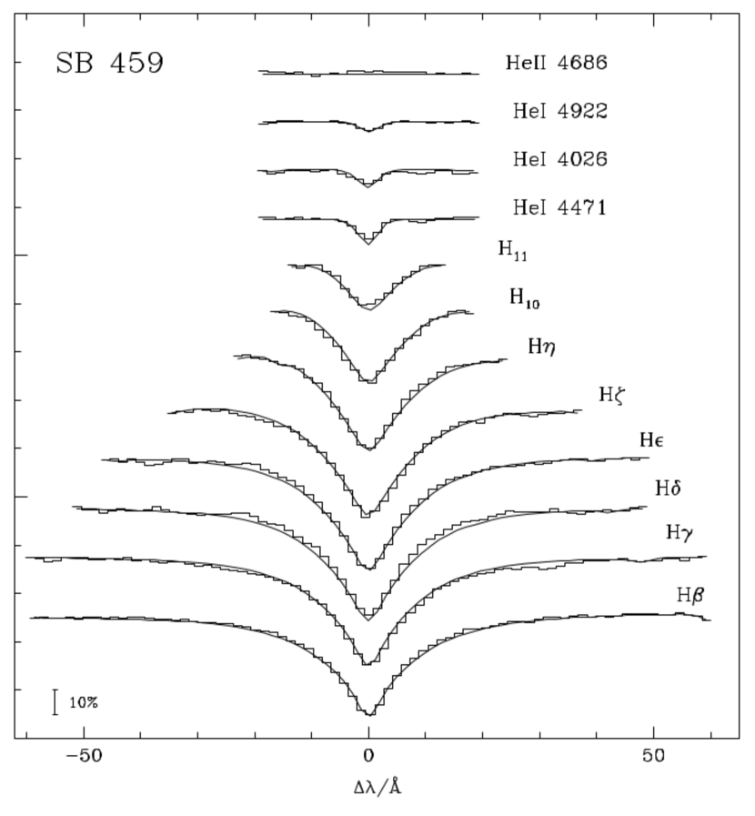
Figure 1: Spectral line fit of the Dupont spectrum of SB 459.

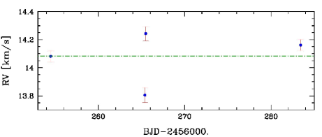
Figure 2: Radial velocities of PG 0342+026. Although four measurements are not enough to fit the RV data with the main pulsation frequencies, at least they give a rough estimate of the RV amplitudes involved.

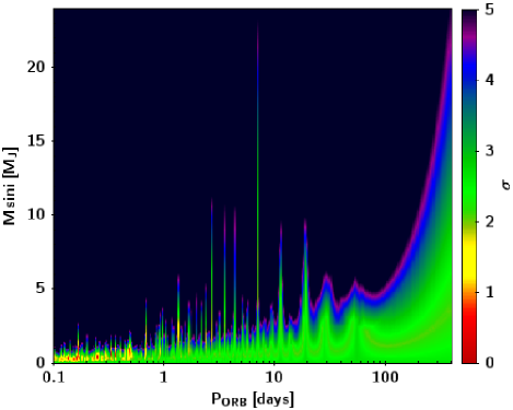
Figure 3: Upper limits to the mass of a hypothetical companion to PG 0342+026 as a function of orbital period. The regions where the presence of a companion is more compatible with the RV measurements are those in red/yellow/green, while the regions in dark blue correspond to a very low probability to have a companion. See text for more details.

PG 0342+026 was observed in November-December 2012 with Harps-N at the Telescopio Nazionale Galileo (TNG, La Palma) in the context of a program to search for sdB low-mass companions (see Silvotti et al. (2020) for more details). Four high-resolution spectra were collected with a mean signal-to-noise ratio of 71 at 4700 Å. Using the cross correlation function on about 150 absorption lines (excluding H and He lines that are too broad), we computed the radial velocities (RV) of the star and we found a mean system velocity of +14.07 km/s with significant variations around this value (Fig. 2). Thanks to the TESS observations, we can now confirm that these variations are at least partly caused by g-mode pulsations, as it has been suspected since 2012. Having available only four RV data points, and knowing that this star pulsates in at least 20 frequencies, we are unable to obtain a reliable fit, however these data can be used to derive an upper limit to the minimum mass (M sin$i$) of a hypothetical companion. The question whether this sdB star is single or not is important for its evolution prior to EHB.

In order to set upper limits to the mass of a companion, we computed a series of synthetic RV curves for different orbital periods and companion masses, assuming circular orbits, and compared these curves with the RV measurements. For each synthetic RV curve we selected the phase that gives the best fit to the data using a weighted least squares algorithm. For each observational point we computed the difference, in absolute value and in $\upsigma$ units (where $\upsigma$ is the observation error), between observed and synthetic RV values. The color coding in Fig. 3 corresponds to the mean value of this difference in $\upsigma$ units. We should keep in mind, however, that these upper limits to the mass of a companion are likely overestimated given that most if not all the variations that we see in Fig. 2 are likely caused by pulsations.

3 Spectral energy distribution, interstellar reddening and stellar parameters

Photometric measurements allow the angular diameters to be determined along with the interstellar extinction, once the atmospheric parameters are known. We constructed spectral energy distributions from photometric measurements ranging from the ultraviolet (IUE) to the infrared. Infrared data were taken from 2MASS, VISTA-VIKING (J,H,K; Skrutskie et al., 2006) and WISE (W1,W2, Cutri & et al., 2012) catalogs. Magnitudes and colours in the Johnson (Allard et al., 1994; Mermilliod et al., 1997; Landolt, 2007), Strömgren (Wesemael et al., 1992; Paunzen, 2015), APASS (Henden et al., 2015), SkyMapper (Wolf et al., 2018), and Gaia (Gaia Collaboration et al., 2018) photometric systems were fitted (for details see Heber et al., 2018). Three numerical box filters were defined to derive UV-magnitudes from IUE UV spectra covering the spectral ranges $1300$–$1800$ Å, $2000$–$2500$ Å, and $2500$–$3000$ Å. Interstellar extinction is accounted for using the extinction curve of Fitzpatrick (1999).

The angular diameter and the interstellar reddening parameter E(B-V) were the only free parameter in the matching of the synthetic the SEDs to the observed ones. In Figure 4 we plot the SEDs as flux density times the wavelength to the power of three (F${}_{\lambda}\lambda^{3}$) versus the wavelength to reduce the steep slope of the SED over such a broad wavelength range. We also display the residuals (O-C) of the magnitudes and the colours. The synthetic SEDs match the observed ones very well in all parts of the wide spectral range. Hence, there is no contribution from potential companions at any wavelength for all three stars. Interstellar reddening is consistent with zero for SB 459 and SB 815 and small for PG 0342+026, all in accordance with the predictions of the maps of Schlegel et al. (1998) and Schlafly & Finkbeiner (2011). The resulting angular diameters and interstellar reddening parameters are given in Tables 2, 3, and 4.

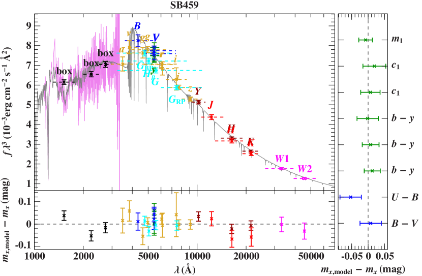
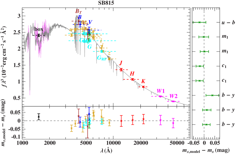
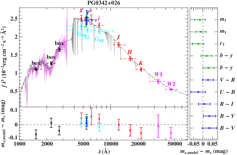
Figure 4: Matching the spectral energy distributions and colours of SB 459 (upper panel), SB 815 (middle panel), and PG0342+026 (lower panel). The colored observed magnitudes (IUE box: black, SDSS: blue; SkyMapper: yellow; Gaia: cyan; VISTA: dark red; 2MASS: red, WISE:magenta) were derived from filter-averaged fluxes. The dashed horizontal lines indicate the filter widths). A model SED calculated with the spectroscopic parameters is overplotted as a solid gray line. Also overlayed are the IUE spectra in magenta. The panels below (SED) and to the right (colours) of the main panel show the residuals for the magnitudes and colours.

Table 2: SB 459: Angular diameters, interstellar reddening parameter, Gaia parallax, and stellar parameters.

Object: SB459	68% confidence interval
Angular diameter $\log(\Theta\,\mathrm{(rad)})$	$-10.6134\pm 0.0016$
Color excess $E(B-V)$	$0.0049\pm 0.0021$ mag
Parallax $\varpi$ (Gaia, $\text{RUWE}=1.17$)	$2.37\pm 0.07$ mas
Effective temperature $T_{\mathrm{eff}}$ (prescribed)	$24900\pm 500$ K
Surface gravity $\log(g\,\mathrm{(cm\,s^{-2})})$ (prescribed)	$5.35\pm 0.10$
Helium abundance $\log(n(\textnormal{He}))$ (fixed)	$-2.58$
Radius $R_{\star}$	$0.228\pm 0.007$ $R_{\odot}$
Mass $M_{\star}$	$0.42\pm 0.11$ $M_{\odot}$
Luminosity $\log\left(\frac{L}{L_{\odot}}\right)$	$1.25\pm 0.05$

Table 3: Same as Table 2, but for SB 815

Object: SB815	68% confidence interval
Angular diameter $\log(\Theta\,\mathrm{(rad)})$	$-10.3920^{+0.0018}_{-0.0017}$
Color excess $E(B-V)$	$0.0018^{+0.0025}_{-0.0018}$ mag
Parallax $\varpi$ (Gaia, $\text{RUWE}=1.23$)	$4.07\pm 0.10$ mas
Effective temperature $T_{\mathrm{eff}}$ (prescribed)	$27200\pm 550$ K
Surface gravity $\log(g\,\mathrm{(cm\,s^{-2})})$ (prescribed)	$5.39\pm 0.10$
Helium abundance $\log(n(\textnormal{He}))$ (fixed)	$-2.94$
Radius $R_{\star}$	$0.221\pm 0.005$ $R_{\odot}$
Mass $M_{\star}$	$0.44\pm 0.11$ $M_{\odot}$
Luminosity $\log\left(\frac{L}{L_{\odot}}\right)$	$1.38\pm 0.05$

Table 4: Same as Table 2, but for PG0342+026

Object: PG0342+026	68% confidence interval
Angular diameter $\log(\Theta\,\mathrm{(rad)})$	$-10.2975\pm 0.0025$
Color excess $E(B-V)$	$0.128\pm 0.004$ mag
Parallax $\varpi$ (Gaia, $\text{RUWE}=1.28$)	$6.13\pm 0.13$ mas
Effective temperature $T_{\mathrm{eff}}$ (prescribed)	$26000\pm 1100$ K
Surface gravity $\log(g\,\mathrm{(cm\,s^{-2})})$ (prescribed)	$5.59\pm 0.12$
Helium abundance $\log(n(\textnormal{He}))$ (fixed)	$-2.69$
Radius $R_{\star}$	$0.182\pm 0.004$ $R_{\odot}$
Mass $M_{\star}$	$0.47\pm 0.14$ $M_{\odot}$
Luminosity $\log\left(\frac{L}{L_{\odot}}\right)$	$1.13\pm 0.08$

In its second data release the Gaia mission (Gaia Collaboration et al., 2018) provided trigonometric parallaxes of high precision (to better than 3%) for all three stars. The “renormalized unit weight error” (RUWE, see Lindegren, 2018) is a good quality indicator for the astrometric solution, because it is independent of the color of the object. This makes it the best choice to judge the quality of the Gaia parallaxes of blue stars, such as studied here. The RUWE value is below the recommended value of $1.4$ for all three stars, indicating that the astrometric solutions are reliable. The Gaia parallaxes and the angular diameters allow us to convert the atmospheric parameters to stellar radii via $R_{\star}\,=\,\Theta/(2\varpi)$, masses via $M_{\star}=gR_{\star}^{2}/G$, and luminosities via $\log\left(\frac{L}{L_{\odot}}\right)\,=\,\log\left(\left(\frac{R_{\star}}{R_{\odot}}\right)^{2}\left(\frac{T_{\mathrm{eff}}}{5775\,\mathrm{K}}\right)^{4}\right)$. The results are summarized in Tables 2, 3, and 4. Uncertainties of the derived radii and luminosities are small because of the high precision of the Gaia parallaxes and well constrained effective temperatures. The derived masses, however, have larger uncertainties resulting from the uncertainties of the spectroscopic surface gravities. The resulting masses are close to canonical (Dorman et al., 1993), but uncertainties are large, mainly due to the surface gravity not yet being sufficiently constrained.

4 Light variations

All three targets have been observed during single TESS sectors, which are specifically listed in Table 1, and have been observed in the short cadence (SC) mode, lasting 120 s. We performed our analysis by using the corrected time series data extracted through the TESS data processing pipeline developed by NASA’s Science Processing Operation Centre. These processed data are publicly available in the Mikulski Archive for Space Telescopes database. We collected these files and have done further analysis. We extracted PDCSAP_FLUX, which is corrected for on-board systematics and neighbors’ contribution to the overall flux. We clipped fluxes at 5$\upsigma$ to remove outliers, de-trended long term variation (longer than days). Finally, we normalized fluxes by calculating $(f/<f>-1)*1000$, deriving part per thousand (ppt). We show the resultant light curves of each target in the top panels of Figure 5.

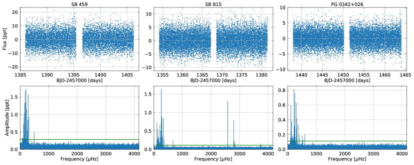
Figure 5: The upper panels show the light curves, while the bottom panels show the amplitude spectra. The green horizontal line in the bottom panels denotes 4.5$\upsigma$ threshold.

4.1 Fourier Analysis

We used a Fourier technique for identifying the frequency of pulsations. Since we have only about 27 days long SC data for each target, the frequency resolution is 0.64 ${\mu}$Hz as defined by 1.5/T, where T is the time coverage of the data (Baran, 2012). The standard prewhitening procedure has been used by fitting the peaks with $A_{i}\sin(2{\pi}f_{i}t+{\phi_{i}})$ by means of a non-linear least-square method. We have used our custom pipeline for this purpose. We prewhitened the data down to the detection threshold defined as 4.5 times the mean noise level, i.e. the signal to noise ratio, S/N = 4.5, calculated from the residual amplitude spectra. The threshold has been discussed by Baran et al. (2015); Zong et al. (2016), who reported slightly higher threshold than in case of ground-based data.The SC mode sampling translates to the Nyquist frequency of 4166 $\upmu$Hz. In case of SB 815 we found some frequencies in the p-mode range, close to the Nyquist frequency and, following a discovery of a reflection across Nyquist (Baran et al., 2012), we also searched the amplitude spectrum above the Nyquist frequency in order to see if any of subNyquist p-modes have superNyquist origin. An amplitude and a profile of the peaks in the sub and superNyquist regions help identifying the origin of the signal. Since the Nyquist frequency is not fixed in time, the reflections will look smeared out and therefore lower in amplitude, however this effect works best if the satellite motion covers substantial part of the orbit, which does not happen in case of single sector data. Therefore, we assume that all frequencies in the p-mode region originate in the subNyquist range are real, but this should be confirmed with shorter cadence data, presumably during the second phase of TESS mission, when 20 sec cadence will be accessible.

In SB 459, we detected 22 frequencies above the detection threshold with 207.314 $\upmu$Hz being the highest amplitude one at 1.72 ppt, and all are in the g-mode region. In SB 815 we detected 37 frequencies in the g-mode region and six frequencies in the p-mode region, with the highest amplitude (1.642 ppt) frequency at 258.1878 $\upmu$Hz. In PG 0342+026, we detected 27 frequencies, with 219.274 $\upmu$Hz having the highest amplitude of 0.758 ppt. We list all frequencies detected in those three stars in Tables 5, 6 and 7.

SB 815 turned out to be a hybrid pulsator. The highest amplitude of 1.296 ppt in the p-mode region shows at 2582.8740 $\upmu$Hz. The signal at high frequencies is parted into two groups. The first one contains four frequencies, while the second one has two low amplitude frequencies. We found the separation between these two groups to be around 896 $\upmu$Hz. Such spacing has been previously reported by (Baran et al., 2009), who concluded that such groups may represent modes with two consecutive radial orders.

Table 5: List of frequencies detected in SB 459

ID	Frequency	Period	Amplitude	S/N	l	n
	[$\upmu$Hz]	[s]	[ppt]
f1	77.82(5)	12849.8(9.0)	0.30(5)	4.5
f2	100.092(48)	9990.8(4.7)	0.34(5)	5.2	1	39
f3	122.319(22)	8175.3(1.5)	0.74(5)	11.1	1/2	32/55
f4	126.27(5)	7919.5(3.3)	0.31(5)	4.6	1	31
f5	140.180(19)	7133.7(10)	0.86(5)	12.9	1	28
f6	145.213(17)	6886.4(8)	0.97(5)	14.6	1	27
f7	156.802(13)	6377.5(5)	1.30(5)	19.6	1/2	25/43
f8	163.519(48)	6115.5(1.8)	0.34(5)	5.1	1	24
f9	178.170(10)	5612.63(31)	1.66(5)	24.9	1	22
f10	196.322(12)	5093.67(31)	1.36(5)	20.4	1	20
f11	207.314(9)	4823.61(22)	1.72(5)	25.8	1	19
f12	221.87(5)	4507.2(1.1)	0.30(5)	4.6
f13	233.175(14)	4288.63(26)	1.17(5)	17.6	1	17
f14	234.566(42)	4263.2(8)	0.39(5)	5.9
f15	242.460(42)	4124.4(7)	0.39(5)	5.9	2	28
f16	246.917(46)	4049.9(8)	0.35(5)	5.3	1	16
f17	251.341(32)	3978.7(5)	0.51(5)	7.7	2	27
f18	261.184(28)	3828.72(40)	0.60(5)	9.0	2	26
f19	263.905(20)	3789.24(28)	0.84(5)	12.6	1	15
f20	286.201(10)	3494.05(13)	1.58(5)	23.7	1	14
f21	309.779(17)	3228.11(18)	0.93(5)	14.0	1/2	13/22
f22	492.395(34)	2030.89(14)	0.47(5)	7.1	2	14

Table 6: List of frequencies detected in SB 815

ID	Frequency	Period	Amplitude	S/N	l	n
	[$\upmu$Hz]	[s]	[ppt]
f1	100.438(7)	9956.4(7)	0.718(21)	27.3	1	38
f2	103.574(39)	9655.0(3.6)	0.125(21)	4.8	1	37
f3	106.159(34)	9419.8(3.0)	0.141(21)	5.4	1/2	36/62
f4	112.435(31)	8894.0(2.4)	0.228(22)	8.7
f5	112.789(24)	8866.1(1.9)	0.291(22)	11.1	1	34
f6	123.734(32)	8081.9(2.1)	0.149(21)	5.7	1	31
f7	128.523(22)	7780.7(1.3)	0.217(21)	8.3	1	30/t
f8	131.737(20)	7590.9(1.2)	0.242(21)	9.2	1/2	29/50
f9	136.885(9)	7305.4(5)	0.534(22)	20.3	1	28
f10	137.674(27)	7263.5(1.4)	0.186(22)	7.1	2	48
f11	142.334(26)	7025.7(1.3)	0.193(22)	7.3	1	27
f12	142.858(26)	6999.9(1.3)	0.189(22)	7.2
f13	151.999(14)	6579.0(6)	0.345(21)	13.1	1	25/t
f14	154.178(37)	6486.0(1.5)	0.132(21)	5.0
f15	165.197(16)	6053.4(6)	0.306(21)	11.6	2	40
f16	174.841(36)	5719.5(1.2)	0.133(21)	5.1	1	22
f17	182.576(20)	5477.2(6)	0.238(21)	9.0	1	21
f18	202.345(27)	4942.1(7)	0.179(21)	6.8	1	19
f19	213.908(7)	4674.92(16)	0.671(21)	25.6	1/2	18/31
f20	226.812(15)	4408.93(29)	0.328(21)	12.5	1	17
f21	228.836(39)	4369.9(7)	0.123(21)	4.7	2	29
f22	236.890(10)	4221.36(17)	0.489(21)	18.6	2	28
f23	246.268(38)	4060.6(6)	0.125(21)	4.8	2	27
f24	258.1879(29)	3873.149(44)	1.642(21)	62.5	1	15
f25	266.359(24)	3754.33(33)	0.204(21)	7.8	2	25
f26	273.537(5)	3655.82(7)	0.878(21)	33.4	1	t
f27	277.625(34)	3601.99(44)	0.143(21)	5.4	2	24
f28	279.723(6)	3574.96(8)	0.777(21)	29.6	1	14
f29	285.303(34)	3505.05(42)	0.141(21)	5.4
f30	289.809(14)	3450.55(16)	0.353(21)	13.4	2	23
f31	302.183(37)	3309.26(40)	0.137(22)	5.2
f32	302.892(14)	3301.51(16)	0.353(22)	13.4	1/2	13/22
f33	330.565(6)	3025.12(5)	0.848(21)	32.3	1	12
f34	361.604(19)	2765.46(14)	0.257(21)	9.8	1	11
f35	445.775(40)	2243.29(20)	0.121(21)	4.6	1	9
f36	482.523(40)	2072.44(17)	0.119(21)	4.5	2	14
f37	669.836(19)	1492.902(42)	0.255(21)	9.7
f38	2582.8740(37)	387.1656(6)	1.296(21)	49.3
f39	2793.905(6)	357.9219(8)	0.786(21)	29.9
f40	2808.165(22)	356.1045(28)	0.214(21)	8.1
f41	2841.082(31)	351.9786(39)	0.153(21)	5.8
f42	3737.134(28)	267.5848(20)	0.169(21)	6.4
f43	3747.579(40)	266.8390(29)	0.118(21)	4.5

Table 7: List of frequencies detected in PG 0342+026

ID	Frequency	Period	Amplitude	S/N	l	n
	[$\upmu$Hz]	[s]	[ppt]
f1	96.786(35)	10332.1(3.7)	0.145(21)	5.5
f2	108.889(9)	9183.7(7)	0.593(21)	22.6	1/2	40/69
f3	114.621(23)	8724.4(1.7)	0.222(21)	8.5	1	38
f4	124.720(42)	8018.0(2.7)	0.120(21)	4.6	1	35
f5	128.559(32)	7778.5(1.9)	0.161(21)	6.1	1	34
f6	132.313(32)	7557.8(1.8)	0.160(21)	6.1	1	33
f7	136.448(13)	7328.8(7)	0.391(21)	14.9	1	32
f8	145.763(28)	6860.5(1.3)	0.185(21)	7.0	1	30
f9	150.803(39)	6631.2(1.7)	0.131(21)	5.0	1	29
f10	156.352(34)	6395.8(1.4)	0.152(21)	5.8	1	28
f11	175.286(30)	5705.0(10)	0.170(21)	6.5	1/2	25/43
f12	198.546(36)	5036.6(9)	0.141(21)	5.4	2	38
f13	204.375(30)	4893.0(7)	0.167(21)	6.3	2	37
f14	219.274(6)	4560.50(13)	0.819(21)	31.1	1	20
f15	231.527(17)	4319.16(32)	0.298(21)	11.3	1	19
f16	243.921(17)	4099.69(28)	0.307(21)	11.7	1/2	18/31
f17	250.256(7)	3995.90(11)	0.758(21)	28.8	1	t
f18	260.620(30)	3837.00(45)	0.167(21)	6.4	1/2	17/29
f19	295.891(8)	3379.62(9)	0.623(21)	23.7	1	15
f20	303.246(28)	3297.65(30)	0.181(21)	6.9	2	25
f21	315.536(20)	3169.21(20)	0.252(21)	9.6	2	24
f22	318.907(13)	3135.71(13)	0.390(21)	14.8	1	14
f23	359.953(15)	2778.14(12)	0.329(21)	12.5	1	t
f24	406.920(26)	2457.48(16)	0.194(21)	7.4	1	11
f25	510.726(28)	1958.00(11)	0.182(21)	6.9	1/2	9/15
f26	529.408(43)	1888.90(15)	0.119(21)	4.5
f27	597.478(25)	1673.70(7)	0.204(21)	7.8

4.2 Multiplets

Multiplets are a result of stellar rotation that changes frequency of modes with the same modal degree and m$\neq$0. The frequency change also depends on a rotation period of a star. For a given modal degree l there is 2l + 1 components differing in an azimuthal order m, therefore by the number of components in an identified multiplet we can infer the modal degree.

We could not detect multiplets in any of these three targets. The reason for null detection may be not long enough data coverage, which causes the frequency resolution not to be high enough to resolve multiplet components. A common rotation period derived in sdB stars is around 40 days (e.g. Baran et al., 2012; Baran & Winans, 2012; Telting et al., 2012; Østensen et al., 2014; Foster et al., 2015; Charpinet et al., 2018), which, in case of p-modes, translates to 0.29$\upmu$Hz or half the frequency resolution of our data, though exceptions are found (Baran et al., 2009; Reed et al., 2014). Another explanation may be a pole-on orientation of a pulsation axis, however we consider this explanation to be very unlikely, since we do not expect all three randomly chosen targets to be oriented in exactly the same way. In case the amplitudes of the side components are low, below the detection threshold, these components will not be detected, either.

4.3 Asymptotic Period Spacing

Another method that helps identifying modes relies on periods and not frequencies. In the asymptotic limit, i.e. n$\gg$l, consecutive overtones of g-modes are nearly equally spaced in period (e.g. Charpinet et al., 2000; Reed et al., 2011). The pulsation period of a given mode with degree l and radial order n can be expressed as

$$P_{l,n}=\frac{P_{0}}{\sqrt{l(l+1)}}n+\epsilon$$ (1)

where $P_{0}$ is the period of the fundamental radial mode and $\epsilon$ is an offset (Unno et al., 1979). Thus, for two consecutive radial overtones and a given modal degree, a difference (commonly called as period spacing) of their periods should be constant, dependent of the modal degree and independent of the radial order.

$${\Delta}P_{l}=P_{l,n+1}-P_{l,n}=\frac{P_{0}}{\sqrt{l(l+1)}}$$ (2)

Using Equation 1 it is possible to assign the radial order n to the precision of some arbitrarily chosen offset $n_{l}$. We provide those values in Tables 5,6 and 7. Using Equation 2 we can also derive a ratio between a period spacing of modes of different modal degree, e.g. the ratio between dipole and quadrupole modes equals 1/$\sqrt{\rm 3}$. This is very strong constraint, since having the period spacing for dipole modes, we can estimate the expected value for higher degree modes. Previous analyses of photometric space data of sdBVs show that the average period spacing of dipole modes is nearly 250 s on average (Reed et al., 2018a). The average spacing for quadrupole modes is found to be close to the expected value, being a result of the ratio given above.

Best, if the mode identification is done based on both features, multiplets and period spacing, since they complement each other providing more convincing conclusion on a mode assignment, very often helping to start finding a specific modal degree sequence. In our case, we had to rely solely on the period spacing. We started our modal degree assignment with the highest amplitude modes. This assumption is justified by the surface cancellation effect, which causes that modes with higher degrees have smaller observational amplitudes. In this consideration, it is assumed that all modes have the same intrinsic amplitudes, which may not necessarily be correct, however our thus far experience clearly shows that most of the high amplitude frequencies in sdBV stars are dipole modes. Despite of this assumption, if two peaks satisfy both dipole and quadrupole sequences, we mentioned both values in tables and figures. In échelle and reduced period diagrams we have added these points with different color coding. The average period spacing in sdBVs detected thus far is between 200 and 300 sec. To guess the average spacing in our targets, we calculated the Kolmogorov-Smirnov (KS) test and we plotted the results in Figure 6. The meaning of a Q value and more details on this test is provided by Kawaler (1988). Basically, this test provides the most common values of period spacings that exist in the data. The result of our mode identification based on the asymptotic period spacing is also presented in échelle diagrams, which we discuss in Section 4.4.

SB 459
The KS test shows a common spacing of periods around 260 s shown in the left panel of Figure 6. We identified 12 dipole modes, four quadrupole modes and three peaks satisfying both sequences. We marked them in the amplitude spectrum in Figure 7. Linear fits provide the average period spacings of 259.16(56) s and 149.89(5) s for dipole and quadrupole modes, respectively.

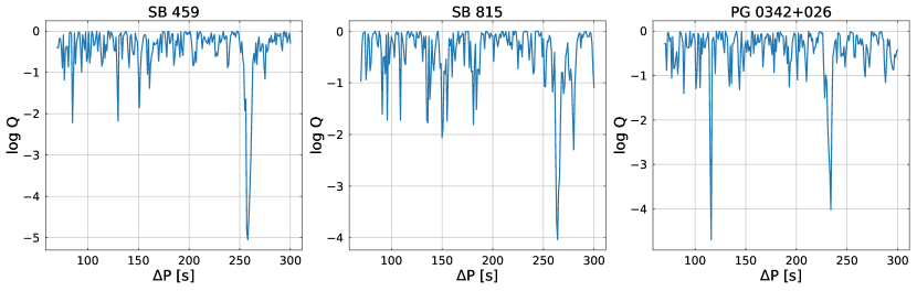
Figure 6: Kolmogorov-Smirnov test for SB 459, SB 815 and PG 0342+026

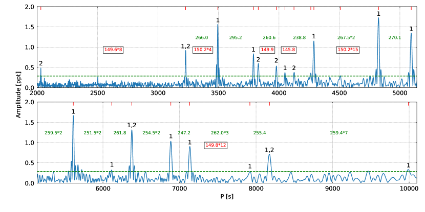
Figure 7: A close-up of the amplitude spectrum of SB 459 plotted in period instead of frequency. The green horizontal dashed line denotes the 4.5$\upsigma$ detection threshold. The values of modal degrees are shown on top of each identified modes. The values between frequencies denote period spacing between two overtones of the same degree (green for dipole and boxed red for quadrupole modes).

SB 815
In our analysis, we detected six frequencies in the p-mode region and we excluded those from our KS test, which eventually points at a common spacing of around 264 s (middle panel in Figure 6). We arrived at two possible solutions, which we present in Fig. 11 and 8.
Solution 1:
In this solution, we identified 17 dipole modes, nine quadrupole modes, while four peaks fit both sequences. Linear fits provide the average period spacings of 265.04(73) s and 153.02(11) s for dipole and quadrupole modes, respectively. We identified a frequency 273.537 $\upmu$Hz with an amplitude of 33.4$\upsigma$, where $\upsigma$ denotes an average noise level, which fits neither dipole nor quadrupole sequence. Its amplitude is also much higher to consider it to be any l $\geq$ 3 mode due to the surface cancellation effect (Dziembowski, 1977). Therefore, we assigned it as a trapped dipole mode. This mode identification looks fairly good, but two frequencies 128.523 and 151.999 $\upmu$Hz differ excessively from the mean period spacing (28.5% and 15.6%, respectively). To justify these extreme deviations we followed the theoretical consideration provided by Charpinet et al. (2013) in Figure 4, which presents that thin hydrogen envelope sdBVs show higher deviations from the mean period spacing.
Solution 2:
This solution considers those two extremely deviated frequencies as candidate for trapped modes. These peaks have moderate amplitudes (8.3 and 13.1 $\upsigma$ respectively) and they do not fit the quadrupole sequence any better. Therefore, taking these two as trapped modes sorts out large deviations in the period sequence of the dipole modes. In this solution we are left with 15 dipole modes with average period spacing of 265.15(57) s and three trapped modes.

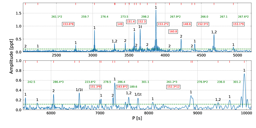
Figure 8: Same as Figure 7 but for SB 815.

PG 0342+026
The KS test points at a common spacing around 232 s (right panel in Figure 6). There is another minimum of a $\log{Q}$ value at 116 sec. It is close to the expected value of a period spacing of quadrupole modes (132 sec), however it is half the period spacing of dipole modes, which sometimes appears in this test. We identified 13 dipole modes, four quadrupole modes and five modes satisfying both sequences. We marked all identified modes in the amplitude spectrum in Figure 9. A linear fit provides the average period spacings 232.25(30) s and 133.74(10) s for dipole and quadrupole modes, respectively. Two frequencies seem to be candidates for trapped modes and we refer to Section 4.4 for more details.

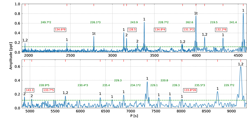
Figure 9: Same as Figure 7 but for PG 0342+026.

We have collected average period spacings ($\Delta$P) as a function of effective temperature for sdBV stars from the literature. All these collected information for 27 sdBVs is provided in Table 8. We plotted these two parameters in Figure 10. We stress that the sample is not very large yet and any conclusion maybe biased. The first try of finding correlation between $\Delta$P and T_eff has been undertaken by Reed et al. (2011) with null result. We increased the number of points but our plot shows that still no clear correlation is present. There are zones of avoidance, though they may just be lacking data points as a consequence of a small sample. Therefore, based on our findings, we conclude that the average period spacing does not correlate with T_eff and so $\Delta$P does not translate to a specific T_eff and vice versa.

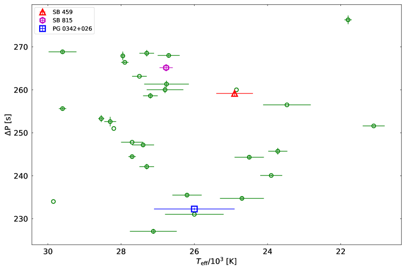
Figure 10: Effective temperature in function of an average period spacing.

4.4 Échelle diagrams and candidates for trapped modes

The échelle diagrams are very useful tools for testing the identification of the modes by means of the asymptotic period spacing. These diagrams represent P mod $\Delta$P in function of P, where P is the pulsation period and $\Delta$P is a period spacing. We present the diagrams for all three targets in Figure 11. For SB 815 we include two solutions. The upper panels show the échelle diagrams for dipole modes while the bottom panels show the diagrams for quadrupole modes. Peaks satisfying both the sequences have been added to both dipole and quadrupole échelle diagrams and represented with green color points. The right vertical axes show the radial orders with respect to an offset $n_{l}$ from the real radial k order. The k number can only be determined from modeling (e.g. Charpinet et al., 2000).

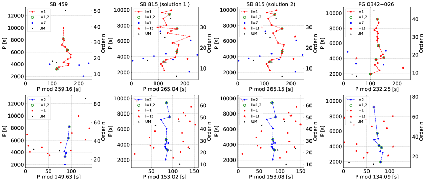
Figure 11: Échelle diagrams for dipole (top panels) and quadrupole (bottom panels) modes. In legends, ‘l=1t’ denotes dipole trapped modes and ‘UM’ denotes undefined modes.

The asymptotic relation, defined by equation 2, is strict only for homogeneous stars. In that case, standing waves of g-modes oscillate in a cavity created e.g. by the convective zone and the surface of a star. Then, the consecutive overtones are spaced equally in period and in an échelle diagram we can see a vertical ridge for a given modal degree. However, in a real star, as the density is not uniform, the ridge almost never becomes purely vertical. Some jitter appears. Since this feature is a consequence of a non uniform structure of a star, deviations from a vertical ridge bear information about a chemical profile and hence cavities. Baran & Winans (2012) reported on a deviation from the vertical ridge, being a common property of many sdB stars (Baran et al., 2019). The so-called a "hook" feature has never been explained thus far but surely must be accounted for if reliable models are to be calculated.

In a few cases, frequencies did not fit well either sequence. The reason may be hidden deep in the sdB interior where the H/He or C/He transition layers between the convective core and the surface appear. These boundaries may contribute to create additional cavities causing some modes to be imprisoned in smaller cavities. Those modes are called trapped modes and they do not follow an asymptotic sequence. The theoretical explanation was provided by Charpinet et al. (2000) and Ghasemi et al. (2017).

There is a "hook" feature in SB 459 between 3 000 and 7 000 s, while in PG 0342+026 the feature is not as pronounced. The largest jitter appears in SB 815 which deviates from the mean period spacing by 28.5%. The upper part of the ridge is not smooth, winding from side to side. That is why we decided to present two solutions for this target. In the absence of multiplets, it is always difficult to make sure that a mode identification is fully correct. Our first solution contains the largest jitter but it provides the "hook" feature in between 3 000 and 7 000 s. In our second solution, we removed two extremely deviated points (6579.0 s and 7780.7 s) from the dipole mode sequence, and marked them as trapped mode candidates. In the latter solution the échelle diagram looks more smooth and still shows the "hook" feature. With no multiplets detected our identification will always suffer from doubts in modal degree assignment, mostly because period spacing sequences of different modal degree cross each other and some of the modes are fitting both sequences fairly well. In case of high amplitude frequencies we prefer l = 1 rather than higher degrees. The ridges of quadrupole modes are fairly short and those modes are mostly leftovers from l = 1 assignment.

One of the best tools to look for trapped modes is a reduced period diagram. The diagram presents a reduced period $\Pi={\rm P}\cdot\sqrt{l(l+1)}$ in function of a reduced period spacing $\Delta\Pi=\Delta{\rm P}\cdot\sqrt{l(l+1)}$. This multiplication causes sequences of all modal degrees to overlap. Overall, the shape of the plot would be similar to what we see in the échelle diagrams, though it will be twisted, so the ridge is now horizontal. Modes with different modal degrees overlap, however, what is more important, the candidates for trapped modes of different degrees also overlap. It can be clearly seen in the papers by e.g. Østensen et al. (2014); Uzundag et al. (2017); Baran et al. (2017). The actual periods of those trapped modes differ between modal degrees, so it is not easy to spot them in amplitude spectra, however the multiplicative factor brings them all in one place in this diagram.

We show the reduce period diagrams for two targets, SB 815 (two solutions) and PG 0342+026 in Figure 12. In SB 459, the sequence of quadrupole modes is too short, not pointing at any trapped mode candidates, which makes the diagram completely inconclusive, and that is why we decided not to present it. In the first solution of SB 815 and in PG 0342+026, the candidates for trapped modes appear to be at the shortest periods. It looks similar to the diagrams reported by the other authors mentioned above. In SB 815 we find either one (solution 1) or three (solution 2), while in PG 0342+026 we find two candidates for trapped modes. Two longest periods trapped modes in SB 815 (solution 2) and two trapped modes in PG 0342+026 are separated by almost 2 000 sec. It agrees with values reported by the other authors and calculated from theoretical considerations reported by Charpinet et al. (2000). Unluckily, in PG 0342+026 the quadrupole sequence do not extend to overlap with those candidates and therefore we cannot confirm trapped mode identification. Likewise in SB 815 (solution 1). In the case of solution 2, although the dipole and quadrupole sequences overlap, we detected no quadrupole trapped modes candidates. This makes those dipole trapped modes candidates less reliable. They can still serve as an additional constraint in modeling, help deriving the most reliable solution and understand the chemical profile inside sdB stars, which is responsible for trapped modes.

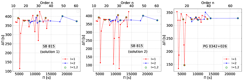
Figure 12: Reduced period diagrams for SB 815 and PG 0342+026. See text for more details.

5 Evolutionary status

The stellar atmospheric parameters such as effective temperature T_eff and surface gravity $\log{g/(\rm{cm\,s^{-2}}}$) have great importance to determine physical conditions of stellar atmospheres. We have taken these two spectroscopic parameters of all sdBVs known to date from Holdsworth et al. (2017) and for our three TESS targets from Table 1. We have plotted these three targets along with 118 other previously known sdBVs in the effective temperature - surface gravity diagram (Figure 13). In the plot we can distinguish three different regions i.e. low T_eff and $\log{g/(\rm{cm\,s^{-2}}}$) containing g-mode pulsators (shown in cyan squares), high T_eff and $\log{g/(\rm{cm\,s^{-2}}}$) containing p-mode pulsators (shown in black circles), and the hybrid pulsators region (shown in magenta triangles) containing pulsators that show both p- and g-modes. Three TESS targets have been shown with bigger symbols along with the error bars. SB 459 and PG 0342+026 are located among g-mode pulsators, which is consistent with the frequency content of these two stars. The amplitude spectrum of SB 815 contains both g-mode and p-mode, which is also confirmed by its location in the plot.

Table 8: Effective temperature and average period spacing data for known sdBVs. The first reference is for $\Delta$ P and the second is for T_eff. References: 1. Reed et al. (2018a), 2. Silvotti et al. (2019), 3. Reed et al. (2011), 4. Holdsworth et al. (2017), 5. Sanjayan et al. (in preparation), 6. Charpinet et al. (2019), 7. Reed et al. (2020) (submitted)

Name	$\Delta$P [s]	Teff [kK]	References
KIC 1718290	276(1)	21.8(1)	1,4
KIC 2437937	234.73(52)	24.7(6)	5,4
KIC 2438324	235.49(51)	26.2(4)	5,4
KIC 2569576	244.31(46)	24.5(4)	5,4
KIC 2697388	240.06(19)	23.9(3)	1,4
KIC 2991403	268.52(74)	27.3(2)	1,4
KIC 3527751	266.4(2)	27.9(1)	1,4
KIC 5807616	242.12(62)	27.3(2)	1,4
KIC 7664467	260.02(77)	26.8(5)	1,4
KIC 7668647	247.8	27.7(3)	1,4
KIC 8302197	258.61(62)	27.2(2)	1,4
KIC 9472174	255.63(30)	29.6(1)	1,4
KIC 10001893	268.0(5)	26.7(3)	1,4
KIC 10553698	263.15	27.5(2)	1,4
KIC 10670103	251.6(2)	21.1(3)	1,4
KIC 11179657	231.02(2)	26.0(8)	1,4
KIC 11558725	244.45(32)	27.7(1)	1,4
EPIC 201206621	268(1)	27.954(54)	1,4
EPIC 202065500	234	29.85	1,4
EPIC 203948264	261.34(78)	26.76(61)	1,4
EPIC 211696659	227.05(56)	27.12(64)	1,4
EPIC 211779126	253.3(8)	28.542(82)	1,4
EPIC 212707862	252.6(1.1)	28.298(162)	1,4
EPIC 218366972	251	28.2	1,4
EPIC 218717602	260	24.85	1,4
EPIC 220641886	256.5(1)	23.47(65)	2,2
KPD 0629-0016	247.17(48)	27.4(3)	3,4
TIC 013145616	268.85(32)	29.60(38)	7,7
TIC 278659026	245.71(75)	23.72(26)	6,6

In Fig. 13 we also plotted theoretical evolutionary tracks to assess the evolutionary status of our three targets. The tracks have been calculated using publicly available open source code MESA (Modules for Experiments in Stellar Astrophysics; Paxton et al., 2011; Paxton et al., 2013, 2015, 2018, 2019), version 11701. We started with a pre-main-sequence model of a solar mass star, assumed a proto-solar chemical composition of Asplund et al. (2009) (Z = 0.142, Y = 0.2703), and evolved the model to the tip of the red giant branch. Then, before the helium flash, we removed most of its mass leaving only a residual hydrogen envelope on top of the helium core. The model was then relaxed to an equilibrium state and evolved until the depletion of helium in the core. All physical and numerical details of the models are discussed in Ostrowski et al. (in preparation). The models use predictive mixing to ensure proper growth of the convective core during the course of evolution (Paxton et al., 2018). The evolutionary tracks presented in Fig. 13 show stable core He burning phase of the sdB evolution. Different tracks correspond to models with different hydrogen envelope masses ($M_{\rm env}$ = 6 $\times$ 10^-4 – 5 $\times$ 10^-3 $M_{\odot}$). It may be noted that the effect of increasingly more massive hydrogen envelopes is to shift the evolutionary tracks towards lower effective temperatures.

The sdBs start their evolution toward lower effective temperatures and lower surface gravities. The direction of the evolution is reversed when the central helium abundance drops below about 10%. The presented tracks fit the location of all our three targets very well and firmly confirm the three stars to be sdBs. All three targets are located on the He-core burning tracks. SB 459 fits really well to a track with an envelope mass of M_env = 2 $\times$ 10^-3M_⊙ and still has more than half of its initial helium abundance available in the core. SB 815 is more advanced in its evolution with a central helium abundance of about ten percent and it is better fitted by a track with an envelope mass of M_env = 1 $\times$ 10^-3M_⊙. The spectroscopic parameters of the star are determined with better precision than those of other two targets. PG 0342+026 seems to be the youngest sdBVs among the three stars, at the beginning of the sdB phase. The envelope mass of the star may vary between M_env = 1 – 3 $\times$ 10^-3M_⊙.

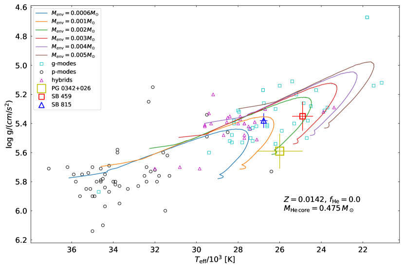
Figure 13: Evolutionary tracks of sdB stars in the $\log{g}$ - $T_{\mathrm{eff}}$ diagram for sdB stars with initial mass of $M_{\mathrm{i}}=1.0\,M_{\odot}$, mass of helium core $M_{\mathrm{He,\,core}}=0.475\,M_{\odot}$ and envelope masses of $6\times 10^{-4}-5\times 10^{-3}$ M_⊙. Observational data are taken from Holdsworth et al. (2017) along with three sdBVs explained in this paper.

6 Summary

In this paper we report our asteroseismic analysis of three sdBV stars observed by the TESS satellite. We have analyzed amplitude spectra to detect pulsation modes and we used the asymptotic period spacing to describe modes’ geometries. For SB 459 we found 12 dipole modes, four quadrupole modes and three modes that can be assigned with either modal degree. For SB 815 we did not find a unique solution. In solution 1 we identified 17 dipole modes, nine quadrupole modes and four modes that can be assigned with either modal degree. In solution 2 we identified the same number of modes, however two dipole modes are considered candidates for trapped modes. In PG 0342+026 we identified 13 dipole modes, four quadrupole modes and five modes that can be assigned with either modal degree. We found none multiplets and therefore our mode identification should be taken with caution.

The average period spacings of dipole modes is around 259 s and 265 s and 232 s for SB 459, SB 815 and PG 0342+026, respectively. In all three targets we detected only few quadrupole modes and hence average period spacing values for quadrupole modes calculated from the linear fits are not too precise. We used a theoretical relation between period spacings of dipole and quadrupole modes, instead.

We also found a few candidates for trapped modes, one/three in SB 815 and two in PG 0342+026. In the reduced period diagrams the trapped mode candidates are spaced by around 2000 sec. This spacing is predicted by theoretical calculations and makes our conclusion more reliable, yet not absolutely convincing, since we detected no quadrupole trapped modes counterparts.

By making use of the high precision Gaia parallaxes and spectral energy distributions from the ultraviolet to the infrared spectral range we derived the fundamental stellar parameters mass, radius, and luminosity from spectroscopically determined effective temperatures and gravities. The results are consistent with the predictions of canonical stellar evolutionary models (Dorman et al., 1993), however, with large uncertainties on stellar mass due to large uncertainties on $\log g$.

The location of our three sdBVs in the effective temperature - surface gravity diagram confirms that SB 459 and PG 0342+026 are g-mode dominated sdBVs and SB 815 is g-mode dominated hybrid pulsator. Theoretical evolutionary tracks provide a coarse-grained approximation of physical properties of these stars like He-core and hydrogen envelope masses, sizes of their cores along with their evolutionary sdB stages. These tracks show that all three stars are during core-helium-burning phase, where SB 815 is much more evolved than other two and PG 0342+026 has just entered the sdB phase.

We also tried to look for any correlation between $\Delta$P and T_eff with all previously known g-mode sdBVs along with our three TESS targets. We found no correlations though. We suspect to see some correlations with increasing data points. The asteroseismic analysis of these targets will help to constrain models for these stars. This paper is our first attempt to list g-mode rich sdBVs observed in TESS and to do mode identifications for these targets.

References

- Allard et al. (1994) Allard F., Wesemael F., Fontaine G., Bergeron P., Lamontagne R., 1994, AJ, 107, 1565
- Altmann et al. (2004) Altmann M., Edelmann H., de Boer K. S., 2004, A&A, 414, 181
- Asplund et al. (2009) Asplund M., Grevesse N., Sauval A. J., Scott P., 2009, ARA&A, 47, 481
- Baran (2012) Baran A., 2012, AcA, 62, 179
- Baran & Winans (2012) Baran A. S., Winans A., 2012, AcA, 62, 343
- Baran et al. (2009) Baran A., et al., 2009, MNRAS, 392, 1092
- Baran et al. (2012) Baran A. S., et al., 2012, MNRAS, 424, 2686
- Baran et al. (2015) Baran A. S., Koen C., Pokrzywka B., 2015, MNRAS, 448, 16
- Baran et al. (2017) Baran A., Reed M., Østensen R., Telting J., Jeffery C., 2017, A&A, 597, 95
- Baran et al. (2019) Baran A., Telting J., Jeffery C., Østensen R., Vos J., Reed M., Vučković M., 2019, MNRAS, 489, 1556
- Brown et al. (1997) Brown T. M., Ferguson H. C., Davidsen A. F., Dorman B., 1997, ApJ, 482, 685
- Charpinet et al. (1997) Charpinet S., Fontaine G., Brassard P., Chayer P., Rogers F. J., Iglesias C. A., Dorman B., 1997, ApJ, 483, 123
- Charpinet et al. (2000) Charpinet S., Fontaine G., Brassard P., Dorman B., 2000, ApJS, 131, 223
- Charpinet et al. (2013) Charpinet S., Van Grootel V., Brassard P., Fontaine G., Green E. M., Randall S. K., 2013, in Montalbán J., Noels A., Van Grootel V., eds, European Physical Journal Web of Conferences Vol. 43, European Physical Journal Web of Conferences. p. 4005
- Charpinet et al. (2018) Charpinet S., Giammichele N., Zong W., Grootel V. V., Brassard P., Fontaine G., 2018, Open Astronomy, 27, 112
- Charpinet et al. (2019) Charpinet S., et al., 2019, A&A, 632, 90
- Cutri & et al. (2012) Cutri R. M., et al. 2012, VizieR Online Data Catalog, 2311
- Dorman et al. (1993) Dorman B., Rood R. T., O’Connell R. W., 1993, ApJ, 419, 596
- Dziembowski (1977) Dziembowski W., 1977, Acta Astronomica, 27, 203
- Fitzpatrick (1999) Fitzpatrick E. L., 1999, PASP, 111, 63
- Fontaine et al. (2012) Fontaine G., Brassard P., Charpinet S., Green E. M., Randall S. K., Van Grootel V., 2012, A&A, 539, 12
- Foster et al. (2015) Foster H., Reed M. D., Telting J. H., Østensen R. H., Baran A. S., 2015, ApJ, 805, 94
- Gaia Collaboration et al. (2018) Gaia Collaboration et al., 2018, A&A, 616, A1
- Geier et al. (2013) Geier S., Heber U., Edelmann H., Morales-Rueda L., Kilkenny D., O’Donoghue D., Marsh T. R., Copperwheat C., 2013, A&A, 557, A122
- Ghasemi et al. (2017) Ghasemi H., Moravveji E., Aerts C., Safari H., Vučković M., 2017, MNRAS, 465, 1518
- Graham & Slettebak (1973) Graham J. A., Slettebak A., 1973, AJ, 78, 295
- Green et al. (1986) Green R. F., Schmidt M., Liebert J., 1986, ApJS, 61, 305
- Han et al. (2002) Han Z., Podsiadlowski P., Maxted P. F. L., Marsh T. R., Ivanova N., 2002, MNRAS, 336, 449
- Heber (2016) Heber U., 2016, PASP, 128, 2001
- Heber et al. (1984) Heber U., Hunger K., Jonas G., Kudritzki R. P., 1984, A&A, 130, 119
- Heber et al. (2000) Heber U., Reid I. N., Werner K., 2000, A&A, 363, 198
- Heber et al. (2018) Heber U., Irrgang A., Schaffenroth J., 2018, Open Astronomy, 27, 35
- Henden et al. (2015) Henden A. A., Levine S., Terrell D., Welch D. L., 2015, in American Astronomical Society Meeting Abstracts #225. p. 336.16
- Holdsworth et al. (2017) Holdsworth D. L., Østensen R. H., Smalley B., Telting J. H., 2017, Monthly Notices of the Royal Astronomical Society, 466, 5020
- Kaluzny & Ruciński (1993) Kaluzny J., Ruciński S. M., 1993, Monthly Notices of the Royal Astronomical Society, 265, 34
- Kawaler (1988) Kawaler S., 1988, in Advances in Helio- and Asteroseismology. IAU Symposium, No. 123. p. 329
- Kilkenny et al. (1997) Kilkenny D., Koen C., O’Donoghue D., Stobie R. S., 1997, MNRAS, 285, 640
- Lamontagne et al. (2000) Lamontagne R., Demers S., Wesemael F., Fontaine G., Irwin M. J., 2000, AJ, 119, 241
- Landolt (2007) Landolt A. U., 2007, AJ, 133, 2502
- Lindegren (2018) Lindegren L., 2018, Re-normalising the astrometric chi-square in Gaia DR2, GAIA-C3-TN-LU-LL-124, www.rssd.esa.int/doc_fetch.php?id=3757412
- Martin et al. (2017) Martin P., Jeffery C. S., Naslim N., Woolf V. M., 2017, MNRAS, 467, 68
- Massey (1997) Massey P., 1997
- Massey et al. (1992) Massey P., Valdes F., Barnes J., 1992
- Mermilliod et al. (1997) Mermilliod J. C., Mermilliod M., Hauck B., 1997, A&AS, 124, 349
- Moehler (2001) Moehler S., 2001, Publications of the Astronomical Society of the Pacific, 113, 1162
- Moni Bidin et al. (2008) Moni Bidin C., Catelan M., Villanova S., Piotto G., Altmann M., Momany Y., Moehler S., 2008, Binaries among Extreme Horizontal Branch Stars in Globular Clusters. p. 27
- Napiwotzki et al. (1999) Napiwotzki R., Green P. J., Saffer R. A., 1999, ApJ, 517, 399
- Németh et al. (2012) Németh P., Kawka A., Vennes S., 2012, MNRAS, 427, 2180
- Østensen et al. (2010) Østensen R. H., et al., 2010, A&A, 513, 6
- Østensen et al. (2014) Østensen R. H., Telting J. H., Reed M. D., Baran A. S., Nemeth P., Kiaeerad F., 2014, A&A, 569, 15
- Paunzen (2015) Paunzen E., 2015, A&A, 580, A23
- Paxton et al. (2011) Paxton B., Bildsten L., Dotter A., Herwig F., Lesaffre P., Timmes F., 2011, ApJS, 192, 3
- Paxton et al. (2013) Paxton B., et al., 2013, ApJS, 208, 4
- Paxton et al. (2015) Paxton B., et al., 2015, ApJS, 220, 15
- Paxton et al. (2018) Paxton B., et al., 2018, ApJS, 234, 34
- Paxton et al. (2019) Paxton B., et al., 2019, ApJS, 243, 10
- Reed et al. (2011) Reed M. D., et al., 2011, MNRAS, 414, 2885
- Reed et al. (2014) Reed M. D., Foster H., Telting J. H., Østensen R. H., Farris L. H., Oreiro R., Baran A. S., 2014, MNRAS, 440, 3809
- Reed et al. (2018a) Reed M., et al., 2018a, Open Astronomy, 27, 157
- Reed et al. (2018b) Reed M., et al., 2018b, Monthly Notices of the Royal Astronomical Society, 483, 2282
- Reed et al. (2020) Reed M. D., et al., 2020, Monthly Notices of the Royal Astronomical Society, 493, 5162
- Ricker et al. (2014) Ricker G. R., et al., 2014, Transiting Exoplanet Survey Satellite (TESS). p. 914320, doi:10.1117/12.2063489
- Saffer et al. (1994) Saffer R. A., Bergeron P., Koester D., Liebert J., 1994, ApJ, 432, 351
- Schlafly & Finkbeiner (2011) Schlafly E. F., Finkbeiner D. P., 2011, ApJ, 737, 103
- Schlegel et al. (1998) Schlegel D. J., Finkbeiner D. P., Davis M., 1998, ApJ, 500, 525
- Schneider et al. (2018) Schneider D., Irrgang A., Heber U., Nieva M. F., Przybilla N., 2018, A&A, 618, A86
- Silvotti et al. (2019) Silvotti R., Uzundag M., Baran A. S., Østensen R. H., Telting J. H., Heber U., Reed M. D., Vŭcković M., 2019, Monthly Notices of the Royal Astronomical Society, 489, 4791
- Silvotti et al. (2020) Silvotti R., Ostensen R. H., Telting J. H., 2020, arXiv preprint arXiv:2002.04545
- Skrutskie et al. (2006) Skrutskie M. F., et al., 2006, AJ, 131, 1163
- Slettebak & Brundage (1971) Slettebak A., Brundage R. K., 1971, AJ, 76, 338
- Telting et al. (2012) Telting J. H., et al., 2012, A&A, 544, 1
- Telting et al. (2014) Telting J. H., et al., 2014, A&A, 570, 129
- Tody (1986) Tody D., 1986, The IRAF Data Reduction and Analysis System. p. 733, doi:10.1117/12.968154
- Tody (1993) Tody D., 1993, IRAF in the Nineties. p. 173
- Unno et al. (1979) Unno W., Osaki Y., Ando H., Shibahashi H., 1979, Tokyo, University of Tokyo Press; Forest Grove, Ore., ISBS, Inc., 1979. 330 p.
- Uzundag et al. (2017) Uzundag M., Baran A., Østensen R., Reed M., Telting J., Quick B., 2017, A&A, 597, 95
- Wesemael et al. (1992) Wesemael F., Fontaine G., Bergeron P., Lamontagne R., Green R. F., 1992, AJ, 104, 203
- Wolf et al. (2018) Wolf C., et al., 2018, Publ. Astron. Soc. Australia, 35, e010
- Zong et al. (2016) Zong W., Charpinet S., Vauclair G., Giammichele N., Van Grootel V., 2016, A&A, 585, 22
- de Boer (1985) de Boer K., 1985, A&A, 142, 321