Full-Duplex MIMO Systems with Hardware Limitations and Imperfect Channel Estimation

Abstract

We consider a bidirectional in-band full-duplex (FD) multiple-input multiple-output (MIMO) system subject to imperfect channel state information (CSI), hardware distortion, and limited analog cancellation capability as well as the self-interference (SI) power requirement at the receiver analog domain so as to avoid the saturation of low noise amplifier (LNA). A novel minimum mean square error (MMSE)-based joint design of digital precoder and combiner for SI cancellation is offered, which combines the well-known gradient projection method and non-monotonicity considered in recent machine-learning literature in order to tackle the non-convexity of the optimization problem formulated in this article. Simulation results illustrate the effectiveness of the proposed SI cancellation algorithm.

I Introduction

With the beginning of the fifth generation (5G) era architected to support individual service categories, in particular enhanced mobile broadband (eMBB), massive machine type communication (mMTC), and ultra-reliable low latency communication (URLLC)), in-band full-duplex (FD) technology, which enables simultaneous transmission and reception on the same time-frequency resource block, has been considered as a promising alternative to its half-duplex (HD) counterpart, as it can be leveraged to jointly tackle different system requirements such as overhead reduction, resource scarcity problem, and demands for higher data rates.

Despite the fact that the concept of FD communications was developed decades ago, wireless FD operation has – due to the overwhelming self-interference (SI) caused by leakage of its own transmitted signals which results from the close proximity between transmit and receive antennas installed on the FD radio – long been considered infeasible in practice until experimental and theoretical research work demonstrating otherwise emerged in the beginning of the 2010s [1, 2, 3, 4, 5, 6, 7]. Motivated by the above, a substantial amount of research contributions to SI cancellation technology in conjunction with multiple-input multiple-output (MIMO) for higher spatial degree of freedoms (DoFs) has been amassed [8, 9, 10, 11, 12, 13, 14], demonstrating theoretical feasibility of the in-band FD operation under the assumption that ideal channel state information (CSI) knowledge and/or radio-frequency (RF) hardware architectures are available. To mention a few examples, the authors in [13] have studied a hybrid analog-digital SI cancellation architecture for FD MIMO systems with fully-connected analog cancellation taps, whereas [15] investigated an interference mitigation scheme aiming at not only the SI but also inter-user interference in a multi-cell multi-user scenario.

However, the performance of SI cancellation mechanisms for FD is bounded not only by channel estimation inaccuracy but also by non-ideal hardware distortions including nonlinearity of power amplifiers (PAs), digital-to-analog converters (DACs), and I/Q mixers, leading to the necessity of incorporating such imperfections into the design of SI cancellation [16]. To make matters worse, it has been argued recently [12, 13, 17, 18, 19, 20, 21, 22] that the architectural and computational complexity as well as the associated energy consumption in order to perform these hybrid digital-analog SI cancellation will be prohibitive as the number of antennas increases, imposing a new challenge on SI cancellation under limited analog cancellation capability.

In order to tackle this difficulty, a low-complexity SI cancellation method subject to limited analog cancellation capability for large-scale FD MIMO systems was proposed in [12], and a new analog cancellation architecture based on tap delay line processing such that the number of analog cancellation taps can be reduced while maintaining the spatial DoF for the desired system performance was introduced in [19]. Leveraging the latter, [20] studied a FD MIMO system equipped with the low-complexity multi-tap analog canceller proposed in [19] under the assumption of perfect CSI and ideal hardware components, which further extended in [21] to an imperfect CSI scenario without considering hardware distortion. Aiming to simultaneously take into account hardware impairments, imperfect CSI and limited hardware complexity for analog SI cancellation, the authors in [23] proposed a low-complexity spatial-temporal SI cancellation design for bidirectional FD MIMO systems.

One of bottlenecks of contributions such as the ones mentioned above is, however, that the SI power level at the receiver analog domain is not properly tuned so as to avoid the saturation of the low noise amplifier (LNA), which is still a major challenge to be conquered. In this paper, we therefore propose an algorithmic solution to the latter problem for bidirectional FD MIMO communications, while taking all the aforementioned issues ($i.e.,$ imperfect CSI, hardware distortion, and limited analog cancellation capability) into consideration.

The remainder of the article is as follows. In Section II, the system model including imperfect CSI and hardware distortion is given, where signal-to-interference-plus-noise ratio (SINR) expressions and the SI power at receiver analog domain are also mathematically described. The problem formulation for the desired SI cancellation will be discussed in Section III, in which the proposed gradient projection based SI cancellation design is also offered. In Section IV, as an illustration, simulation results are given in order to demonstrate the effectiveness of the proposed method. Finally, conclusions and discussions on possible future works are given in Section V.

Notation: Throughout the article, matrices and vectors will be expressed respectively by bold capital and small letters, namely, $\bm{X}$ and $\bm{x}$. The transpose, conjugate, Hermitian and inverse operators will be respectively denoted by $\left(\cdot\right)^{\mathrm{T}}$, $\left(\cdot\right)^{*}$, $\left(\cdot\right)^{\mathrm{H}}$ and $\left(\cdot\right)^{\footnotesize-1}$, while the expectation, the covariance and the Frobenius norm operators will be respectively denoted by $\mathbb{E}\left[{\cdot}\right]$, $\mathbb{V}\left[\cdot\right]$ and $\left\lVert\cdot\right\rVert$. A complex matrix with $a$ columns and $b$ rows is denoted by $\bm{X}\in\mathbb{C}^{a\times b}$, and a complex random scalar variable following the complex Gaussian distribution with mean $\mu$ and variance $\sigma^{2}$ is expressed as $x\sim\mathcal{CN}\left(\mu,\sigma^{2}\right)$. Finally, the matrix containing only the diagonal of $\bm{X}$ will be denoted by ${\rm diag}\!\left({\!\bm{X}\!}\right)\!$ .

II System Model

Consider a bidirectional two-way in-band FD MIMO system shown in Figure 1, where two nodes operating in FD mode exchange information with the support of a digital precoding vector $\bm{v}_{k}\in\mathbb{C}^{N\times 1}$ with $k\in\{1,2\}$, a digital combining vector $\bm{u}_{k}\in\mathbb{C}^{1\times M}$, and a low-complexity multi-tap analog SI cancellation architecture [19], such that each node is capable of suppressing the SI while increasing the intended signal power at the destination node. For the sake of simplicity but loss of generality, each node is assumed to be equipped with $N$ transmit and $M$ receive antennas, respectively. Due to the limited dynamic range of RF components at the nodes, it is assumed that each node suffer from not only inevitable SI caused by own transmitted signals but also nonlinear hardware impairments from non-ideal PAs, DACs and I/Q mixer.

It is further assumed that the transmit power at the $k$-th node is limited ($i.e.,$ $\mathbb{E}\left[{\left\lVert\bm{v}_{k}s_{k}\right\rVert^{2}}\right]\leq P_{k}$) with $s_{k}$ denoting a unit-power symbol transmitted by the $k$-th node, whereas the combining vector $\bm{u}_{k}$ is normalized ($i.e.,$ $\left\lVert\bm{u}_{k}\right\rVert^{2}=1$). Following [19, 23, 9], the low-complexity multi-tap analog SI cancellation at the $k$-th node can be expressed as $\bm{C}_{k}\in\mathbb{C}^{M\times N}$ composed of $N_{\rm tap}$ non-zero components and $MN-N_{\rm tap}$ zeros.

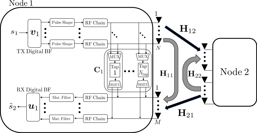
Figure 1: Two-way in-band FD MIMO system model equipped with digital precoder/combiner and multi-tap analog canceller.

Referring to Figure 1, the communication channel from the $\ell$-th node, with $\ell\in\{1,2|\ell\neq k\}$, to the $k$-th node, is denoted by $\bm{H}_{\ell k}\in\mathbb{C}^{M\times N}$ as well as $\bm{H}_{kk}\in\mathbb{C}^{M\times N}$ describing the SI channel at the $k$-th node. In light of the above, the received signal at the $k$-th node after processing by the analog SI cancellation $\bm{C}_{k}$ can be expressed as

$$\bm{y}_{k}\!=\!\underbrace{\bm{H}_{\ell k}\left(\!\bm{v}_{\ell}s_{\ell}+\bm{w}_{\ell}\!\right)}_{\text{Distorted intended signal}}\!\!+\!\overbrace{\bm{H}_{kk}\bm{v}_{k}s_{k}-\bm{C}_{k}\bm{v}_{k}s_{k}+\bm{H}_{kk}\bm{w}_{k}}^{\text{Cancelled \lx@glossaries@gls@link{acronym}{SI}{\leavevmode SI} \& Hardware distortion}}+\bm{n}_{k},$$ (1)

where $\bm{w}_{\ell}\sim\mathcal{CN}\left(\bm{0},\beta\cdot{\rm diag}\left(\bm{v}_{\ell}\bm{v}^{\rm H}_{\ell}\right)\right)$ denotes the nonlinear hardware impairments induced by the $\ell$-th node [16, 24, 25, 26], $\bm{w}_{k}\sim\mathcal{CN}\left(\bm{0},\beta\cdot{\rm diag}\left(\bm{v}_{k}\bm{v}^{\rm H}_{k}\right)\right)$ describes the effect of the self-induced nonlinearity at the $k$-th node, and $\beta$ expresses the hardware distortion level, whereas $\bm{n}_{k}\sim\mathcal{CN}\left(0,\sigma^{2}\mathbf{I}_{M}\right)$ denotes the complex additive white Gaussian noise (AWGN) vector at the $k$-th receiver.

II-A Imperfect CSI model

In this subsection, statistical channel models for the communication and SI channel matrices ($i.e.,$ $\bm{H}_{\ell k}$ and $\bm{H}_{kk}$) will be described, respectively, while introducing the associated imperfection models relying on the Gauss-Markov theorem [27, 28].

Due to the dominant line-of-sight (LoS) stemming from deterministic close proximity between transmit and receive antennas at the FD node, the associated SI channel matrix $\bm{H}_{kk}$ can be modeled as the Rician fading channel [29], namely,

$$\bm{H}_{kk}=\sqrt{\frac{\kappa}{1+\kappa}}\bm{H}^{\rm LOS}_{kk}+\sqrt{\frac{1}{1+\kappa}}\bm{H}^{\rm NLOS}_{kk}\>\>\forall k,$$ (2)

with $\kappa$ denoting the Rician shaping parameter, also referred to as the Rician $K$-factor, which expresses the power contribution of the LoS components relative to non line-of-sight (NLoS) counterparts, while $\bm{H}^{\rm NLOS}_{kk}$ corresponds to sum of NLoS paths such that each element of $\bm{H}^{\rm NLOS}_{kk}$ follows an independent and identically distributed (i.i.d.) complex Gaussian variable with zero mean and unit-variance, and the LoS component $\bm{H}^{\rm LOS}_{kk}$ can be written as a product of phase array responses $\mathbf{a}_{\rm TX}\left(\theta_{T}\right)$ and $\mathbf{a}_{\rm RX}\left(\theta_{R}\right)$ of the transmit and receive antennas, respectively, that is,

$$\bm{H}^{\rm LOS}_{kk}=\alpha_{k}\mathbf{a}^{\rm H}_{\rm RX}\left(\theta_{R}\right)\mathbf{a}_{\rm TX}\left(\theta_{T}\right)\in\mathbb{C}^{M\times N},$$ (3)

where $\alpha_{k}$ is a complex gain, $\theta_{T}$ and $\theta_{R}$ denote the angle of departure (AoD) and angle of arrival (AoA), respectively, and the associated array responses can be written as

$$\mathbf{a}_{\rm TX}\left(\theta_{T}\right) = \left[\begin{array}[]{llll}1&e^{j2\pi d{\rm cos}\left(\theta_{T}\right)}&\cdots&e^{j2\pi d\left(N-1\right){\rm cos}\left(\theta_{T}\right)}\end{array}\right],$$ (5)

$$\mathbf{a}_{\rm RX}\left(\theta_{R}\right) = \left[\begin{array}[]{llll}1&e^{j2\pi d{\rm cos}\left(\theta_{R}\right)}&\cdots&e^{j2\pi d\left(M-1\right){\rm cos}\left(\theta_{R}\right)}\end{array}\right],$$ (7)

where we assume that both FD nodes are equiped with uniform linear array (ULA) with half-wavelength antenna spacing $d$.

Given the above, it is assumed hereafter that CSI knowledge of the communication and SI channel matrices is partially available at the nodes, so that the corresponding imperfect CSI can be expressed via the Gauss-Markov uncertainty model as

$$\bm{H}_{k\ell}\!\!\! = \!\!\!\sqrt{\left(1-\tau^{2}_{k\ell}\right)}\hat{\bm{H}}_{k\ell}+\tau_{k\ell}\bm{E}_{k\ell},$$ (8)

$$\bm{H}_{kk}\!\!\! = \!\!\!\sqrt{\frac{q_{kk}\kappa}{1+\kappa}}\bm{H}^{\rm LOS}_{kk}\!+\!\sqrt{\frac{q_{kk}}{1\!+\!\kappa}\!}\big{(}\sqrt{\!1\!-\!\tau^{2}_{kk}}\hat{\bm{H}}^{\rm NLOS}_{kk}\!\!+\tau_{kk}\bm{E}_{kk}\big{)}$$ (9)

$$= \!\!\!\hat{\bm{H}}_{kk}+\tau^{\prime}_{kk}\bm{E}_{kk},$$

where $\tau_{ij},\>i,j\in\{k,\ell\}$ denote parameters of the CSI accuracy, $\bm{E}_{ij}$ and $\bm{E}_{ii}$ are the channel estimation error matrices with its elements following i.i.d. $\mathcal{CN}\left(0,q_{ij}\right)$ and i.i.d. $\mathcal{CN}\left(0,1\right)$, respectively, where $q_{ij}$ and $q_{ii}$ are the path loss gains of the channels $\bm{H}_{ij}$ and $\bm{H}_{ii}$.

Notice that in equation (9), we implicitly define the known SI components $\hat{\bm{H}}_{ii}$ and the scaled SI CSI accuracy $\tau^{\prime}_{ii}$ for later convenience, which are, respectively, given by

$$\hat{\bm{H}}_{ii} \triangleq \sqrt{\frac{q_{ii}\kappa}{1+\kappa}}\bm{H}^{\rm LOS}_{ii}\!+\!\sqrt{\frac{q_{ii}(1-\tau^{2}_{ii})}{1+\kappa}}\hat{\bm{H}}^{\rm NLOS}_{ii},$$ (10)

$$\tau^{\prime}_{ii} \triangleq \sqrt{\frac{q_{ii}\cdot\tau^{2}_{ii}}{1\!+\!\kappa}\!}.$$ (11)

Furthermore, we considered in equation (9) that perfect (or considerably accurate) knowledge of the LoS component of the SI channel is available due to the deterministic (or much slowly-varying) nature of this channel component [23], implying that only part of the NLoS components possesses uncertainties.

II-B Signal model

Taking into account the imperfect CSI model described in the previous section, plugging equation (8) and (9) into the received signal expression given in equation (1) yields

$$\bm{y}_{k} =\!\overbrace{\sqrt{1\!-\!\tau^{2}_{\ell k}}\hat{\bm{H}}_{\ell k}\!\left(\!\bm{v}_{\ell}s_{\ell}\!+\!\bm{w}_{\ell}\!\right)\!+\!\tau_{\ell k}\bm{E}_{\ell k}\left(\!\bm{v}_{\ell}s_{\ell}\!+\!\bm{w}_{\ell}\!\right)}^{\text{Intended signal with \lx@glossaries@gls@link{acronym}{CSI}{\leavevmode CSI} \& hardware imperfection}}\!$$

$$\hskip 8.61108pt+\!\underbrace{\tilde{\bm{H}}_{kk}\bm{v}_{k}s_{k}+\tau^{\prime}_{kk}\bm{E}_{kk}\left(\bm{v}_{k}s_{k}\!+\!\bm{w}_{k}\right)\!+\!\hat{\bm{H}}_{kk}\bm{w}_{k}}_{\text{Residual \lx@glossaries@gls@link{acronym}{SI}{\leavevmode SI} with \lx@glossaries@gls@link{acronym}{CSI}{\leavevmode CSI} \& hardware imperfection}}+\bm{n}_{k},$$

with $\tilde{\bm{H}}_{kk}\triangleq\hat{\bm{H}}_{kk}-\bm{C}_{k}$ implicitly being defined.

From equation (II-B), the averaged SINR and corresponding mean square error (MSE) at the $k$-th node can be written in a closed-form expression, respectively, as

$$\gamma_{k} = \frac{P_{\mathrm{Com},k}}{\Sigma_{k}},$$ (13)

$$\varepsilon_{k} = \mathbb{E}\left[{\!\left(s_{\ell}-\hat{s}_{\ell}\right)\left(s_{\ell}-\hat{s}_{\ell}\right)^{*}}\right]=\frac{1}{\gamma_{k}},$$ (14)

where the power of the intended signal and interference-plus-noise components can be respectively expressed as

$$P_{\mathrm{Com},k}\!\!\!\! \triangleq \!\!\!\!\left(1\!-\!\tau^{2}_{\ell k}\right)\bm{u}_{k}\hat{\bm{H}}_{\ell k}\bm{v}_{\ell}\bm{v}^{\rm H}_{\ell}\hat{\bm{H}}^{\rm H}_{\ell k}\bm{u}^{\rm H}_{k},$$ (15)

$$\Sigma_{k}\!\!\!\! \triangleq \!\!\!\!\bm{u}_{k}\tilde{\bm{H}}_{kk}\bm{v}_{k}\bm{v}^{\rm H}_{k}\tilde{\bm{H}}^{\rm H}_{kk}\bm{u}^{\rm H}_{k}+{\tau^{\prime}}^{2}_{kk}\left\lVert\bm{v}_{k}\right\rVert^{2}\left(1+\beta\right)$$ (16)

$$\!\!\!\!\!\!\!\!+\beta\bm{u}_{k}\hat{\bm{H}}_{kk}{\rm diag}\!\left({\bm{v}_{k}\bm{v}^{\rm H}_{k}}\right)\!\hat{\bm{H}}^{\rm H}_{kk}\bm{u}^{\rm H}_{k}\!+\!q_{\ell k}\tau^{2}_{\ell k}\left\lVert\bm{v}_{\ell}\right\rVert^{2}\!(1\!+\!\beta)$$

$$\!\!\!\!\!\!\!\!+\beta\left(1-\tau^{2}_{\ell k}\right)\bm{u}_{k}\hat{\bm{H}}_{\ell k}{\rm diag}\!\left({\bm{v}_{\ell}\bm{v}^{\rm H}_{\ell}}\right)\!\hat{\bm{H}}^{\rm H}_{\ell k}\bm{u}^{\rm H}_{k}+\sigma^{2},$$

where the identity $\mathbb{E}\left[{\bm{H}\bm{A}\bm{H}^{\rm H}}\right]=\sigma^{2}{\rm Tr}\left({\bm{A}}\right)\mathbf{I}$ with each element of $\bm{H}$ follows i.i.d. $\mathcal{CN}\left(0,\sigma^{2}\right)$ is leveraged.

Furthermore, for later convenience, the covariance of residual distorted SI after the analog cancellation can be written as

$$\mathbf{\Phi}_{k}\triangleq\mathbb{V}\left[\tilde{\bm{H}}_{kk}\bm{v}_{k}s_{k}+\tau^{\prime}_{kk}\bm{E}_{kk}\left(\bm{v}_{k}s_{k}\!+\!\bm{w}_{k}\right)\!+\!\hat{\bm{H}}_{kk}\bm{w}_{k}\right]$$

$$= \!\!\!\!\!\mathbb{V}\left[\tilde{\bm{H}}_{kk}\bm{v}_{k}s_{k}\right]+\mathbb{V}\left[\tau^{\prime}_{kk}\bm{E}_{kk}\left(\bm{v}_{k}s_{k}\!+\!\bm{w}_{k}\right)\right]+\mathbb{V}\left[\hat{\bm{H}}_{kk}\bm{w}_{k}\right]$$

$$= \!\!\!\!\!\!\tilde{\bm{H}}_{kk}\bm{v}_{k}\bm{v}^{\rm H}_{k}\tilde{\bm{H}}^{\rm H}_{kk}\!\!+\!{\tau^{\prime}}^{2}_{\!\!\!kk}\!\left\lVert\bm{v}_{k}\right\rVert^{\!2}\!\!(1\!+\!\beta)\mathbf{I}\!+\!\beta\hat{\bm{H}}_{kk}\text{diag}(\bm{v}_{k}\bm{v}^{\rm H}_{k})\hat{\bm{H}}^{\rm H}_{kk}.$$

Please note from the above that the diagonal elements of $\mathbf{\Phi}_{k}$ describes the total average SI power at each digital thread at the $k$-th receiver, which therefore need to be sufficiently attenuated before processing by the RF chain so as to avoid saturation of LNA while maintaining the operation point of LNA sufficiently high in terms of energy efficiency of RF circuits. To elaborate, the tunable radio components ($i.e.,$ $\bm{v}_{k}$, $\bm{u}_{k}$, and $\bm{C}_{k}$) need to be designed such that the $m$-th diagonal element $[\mathbf{\Phi}_{k}]_{mm}$ satisfies $[\mathbf{\Phi}_{k}]_{mm}\leq\varepsilon_{k,m}$ with $\varepsilon_{k,m}$ denoting a power level requirement such that the total received signal $\bm{y}_{k}$ enjoys linearity of the dynamic range at the receiver side.

III Proposed SI cancellation design

Taking into account the fact that maximizing SINR at each user corresponds to minimizing the associated MSE as shown in equation (13) and (14), in this section we shall hereafter consider the following sum SINR maximization problem subject to the maximum transmit power constraint at each user as well as the residual SI power level constraints at each RF thread of the receiver, which can be expressed as

$$\!\!\!\!\max_{\bm{v}_{k},\bm{v}_{\ell},\bm{u}_{k},\bm{u}_{\ell}} \!\!\!\!\!\!\!\!g(\bm{v}_{k},\bm{v}_{\ell},\bm{u}_{k},\bm{u}_{\ell})\triangleq\sum^{2}_{k=1}\gamma_{k}$$ (18a)

$${\rm s.t.} \!\!\!\!\!\!\!\!\!\!\left\lVert\bm{v}_{k}\right\rVert^{2}\leq P_{k},\forall k$$ (18c)

$$\!\!\!\!\!\!\!\!\!\![\mathbf{\Phi}_{k}]_{mm}\leq\varepsilon_{k,m},\forall k,m\in\{1,2,\ldots,M\}.$$

One may readily notice that the optimization problem given in equation (18) is an intractable non-convex problem due to not only the non-convexity of the SINR expressions in equation (13) but also the coupling effect between the variables ($i.e.,$ $\bm{v}_{k},\bm{v}_{\ell},\bm{u}_{k}$ and $\bm{u}_{\ell}$). Aiming at relaxing this difficulty while taking advantage of the optimality of linear minimum mean square error (MMSE) receiving filter in case that both the intended signal and the effective interfering signals can be treated as Gaussian [30], we propose a type of the alternating optimization framework in conjunction with the non-monotone algorithmic design [31, 32]. To this end, the normalized MMSE receiving filters at the $k$-th and $\ell$-th node can be, respectively, written in a closed-form expression as

$$\!\bm{u}_{k}\!=\!\tfrac{\bm{v}^{\mathrm{H}}_{\ell}\hat{\bm{H}}^{\mathrm{H}}_{\ell k}\big{(}\!\bm{H}_{\bm{u}_{k}}\bm{H}^{\mathrm{H}}_{\bm{u}_{k}}\!\!+\!{\sigma^{\prime}}^{2}_{\!\!u_{k}}\mathbf{I}_{M}\!+\!(1\!-\!\tau^{2}_{\ell k})\hat{\bm{H}}_{\ell k}\bm{v}_{\ell}\bm{v}^{\rm H}_{\ell}\hat{\bm{H}}^{\rm H}_{\ell k}\big{)}^{\!-1}}{\big{\|}\bm{v}^{\mathrm{H}}_{\ell}\hat{\bm{H}}^{\mathrm{H}}_{\ell k}\big{(}\!\bm{H}_{\bm{u}_{k}}\bm{H}^{\mathrm{H}}_{\bm{u}_{k}}\!\!+\!{\sigma^{\prime}}^{2}_{\!\!u_{k}}\mathbf{I}_{M}\!+\!(1\!-\!\tau^{2}_{\ell k})\hat{\bm{H}}_{\ell k}\bm{v}_{\ell}\bm{v}^{\rm H}_{\ell}\hat{\bm{H}}^{\rm H}_{\ell k}\big{)}^{-1}\big{\|}_{2}},$$ (19a)

$$\bm{u}_{\ell}\!=\!\tfrac{\bm{v}^{\mathrm{H}}_{k}\hat{\bm{H}}^{\mathrm{H}}_{k\ell}\big{(}\!\bm{H}_{\bm{u}_{\ell}}\bm{H}^{\mathrm{H}}_{\bm{u}_{\ell}}\!\!+\!{\sigma^{\prime}}^{2}_{\!\!u_{\ell}}\mathbf{I}_{M}\!+\!(1\!-\!\tau^{2}_{k\ell})\!\hat{\bm{H}}_{k\ell}\bm{v}_{k}\bm{v}^{\rm H}_{k}\hat{\bm{H}}^{\rm H}_{k\ell}\big{)}^{-1}}{\big{\|}\bm{v}^{\mathrm{H}}_{k}\hat{\bm{H}}^{\mathrm{H}}_{k\ell}\big{(}\!\bm{H}_{\bm{u}_{\ell}}\bm{H}^{\mathrm{H}}_{\bm{u}_{\ell}}\!\!+\!{\sigma^{\prime}}^{2}_{\!\!u_{\ell}}\mathbf{I}_{M}\!+\!(1\!-\!\tau^{2}_{k\ell})\!\hat{\bm{H}}_{k\ell}\bm{v}_{k}\bm{v}^{\rm H}_{k}\hat{\bm{H}}^{\rm H}_{k\ell}\big{)}^{-1}\big{\|}_{2}},$$ (19b)

where the effective interfering channels $\bm{H}_{\bm{u}_{k}}$ and $\bm{H}_{\bm{u}_{\ell}}$ are given in equation (20)

$$\bm{H}_{\bm{u}_{k}}\triangleq\left[\tilde{\bm{H}}_{\!kk}\bm{v}_{k},\beta\hat{\bm{H}}_{\!kk}\bm{\Gamma}^{N}_{1}\bm{v}_{k},\beta(1\!-\!\tau^{2}_{\ell k})\hat{\bm{H}}_{\!\ell k}\bm{\Gamma}^{N}_{1}\!\bm{v}_{\ell},\cdots,\beta\hat{\bm{H}}_{\!kk}\bm{\Gamma}^{N}_{N}\bm{v}_{k},\beta(1\!-\!\tau^{2}_{\ell k})\hat{\bm{H}}_{\!\ell k}\bm{\Gamma}^{N}_{N}\bm{v}_{\ell}\right]\!\!$$ (20a)

$$\bm{H}_{\bm{u}_{\ell}}\triangleq\left[\tilde{\bm{H}}_{\!\ell\ell}\bm{v}_{\ell},\beta\hat{\bm{H}}_{\!\ell\ell}\bm{\Gamma}^{N}_{1}\bm{v}_{\ell},\beta(1\!-\!\tau^{2}_{k\ell})\hat{\bm{H}}_{k\ell}\bm{\Gamma}^{N}_{1}\bm{v}_{k},\cdots,\beta\hat{\bm{H}}_{\ell\ell}\bm{\Gamma}^{N}_{N}\bm{v}_{\ell},\beta(1\!-\!\tau^{2}_{k\ell})\hat{\bm{H}}_{k\ell}\bm{\Gamma}^{N}_{N}\bm{v}_{k}\right]\!\!\vspace{-1ex}$$ (20b)

$$\nabla f\left(\bm{v}_{k}\right)=\left(\frac{\partial P_{\mathrm{Com},k}}{\partial\bm{v}^{*}_{k}}\Sigma_{k}-\frac{\partial\Sigma_{k}}{\partial\bm{v}^{*}_{k}}P_{\mathrm{Com},k}\right)\frac{1}{\Sigma^{2}_{k}}+\left(\frac{\partial P_{\mathrm{Com},\ell}}{\partial\bm{v}^{*}_{k}}\Sigma_{\ell}-\frac{\partial\Sigma_{\ell}}{\partial\bm{v}^{*}_{k}}P_{\mathrm{Com},\ell}\right)\frac{1}{\Sigma^{2}_{\ell}},$$ (22)

 

with $\bm{\Gamma}^{N}_{i}\in\mathbb{R}^{N\times N}$ being an all-zero matrix except for its $i$-th diagonal position equal to $1$.

Given fixed receiving filters calculated by equation (19), the optimization problem (18) can then be reduced to

$$\!\!\!\!\max_{\bm{v}_{k},\bm{v}_{\ell}} \!\!\!\!\!\!\!\!f\left(\bm{v}_{k},\bm{v}_{\ell}\right)\triangleq\sum^{2}_{k=1}\gamma_{k}$$ (19a)

$${\rm s.t.} \!\!\!\!\!\!\!\!\!\!\left\lVert\bm{v}_{k}\right\rVert^{2}\leq P_{k},\forall k$$ (19c)

$$\!\!\!\!\!\!\!\!\!\![\mathbf{\Phi}_{k}]_{mm}\leq\varepsilon_{k,m},\forall k,m\in\{1,2,\ldots,M\}.$$

Notice that the residual SI power constraints (19c) are independent from the receiving filters $\bm{u}_{k}$ and $\bm{u}_{\ell}$ since it is needed to be satisfied before processing by the LNA and analog-to-digital converter (ADC), indicating that the precoding vectors must be designed so as to satisfy both the transmit power constraint and (19c) simultaneously. In order to tackle the non-convexity of the objective function (19a) while enjoying the convex sets (19c) and (19c), the FD communication literature [25, 33, 23] as well as recent machine learning research works [31, 32] jointly motivate us to propose an alternating non-monotone gradient projection method described as follows.

A fundamental algorithmic framework of gradient projection methods can be written as

$$\breve{\bm{v}}^{[t]}_{k}\!\! = \!\!\mathcal{P}\Big{\{}\overbrace{\bm{v}^{[t]}_{k}+\delta^{[t]}\nabla f\left(\bm{v}_{k}\right)}^{\triangleq\bar{\bm{v}}_{k}}\Big{\}}$$ (20)

$$\bm{v}^{[t+1]}_{k}\!\! = \!\!\bm{v}^{[t]}_{k}+\rho^{[t]}\left(\breve{\bm{v}}^{[t]}_{k}-\bm{v}^{[t]}_{k}\right)$$ (21)

where $\mathcal{P}\left\{\cdot\right\}$ denotes the projection operator that computes the closest point (in Euclidean sense) from a current estimate towards the feasible set, which is described later in details, $\delta$ and $\rho$ are the intensity parameters for the projection and correction steps, and $\nabla f\left(\bm{v}_{k}\right)$ is the gradient of $f\left(\bm{v}_{k}\right)$, which can be written in a closed-form expression as shown above in equation (22), with

$$\frac{\partial P_{\mathrm{Com},k}}{\partial\bm{v}^{*}_{k}}\!\!\! = \!\!\!\bm{0}_{N\times 1},$$ (23a)

$$\frac{\partial P_{\mathrm{Com},\ell}}{\partial\bm{v}^{*}_{k}}\!\!\! = \!\!\!\left(1\!-\!\tau^{2}_{k\ell}\right)\hat{\bm{H}}^{\rm H}_{k\ell}\bm{u}^{\rm H}_{\ell}\bm{u}_{\ell}\hat{\bm{H}}_{k\ell}\bm{v}_{k},$$ (23b)

$$\frac{\partial\Sigma_{k}}{\partial\bm{v}^{*}_{k}}\!\!\! = \!\!\!\tilde{\bm{H}}^{\rm H}_{kk}\bm{u}^{\rm H}_{k}\bm{u}_{k}\tilde{\bm{H}}_{kk}\bm{v}_{k}+{\tau^{\prime}}^{2}_{kk}\left(1+\beta\right)\bm{v}_{k}$$ (23c)

$$\hskip 8.61108pt+\beta\sum^{N}_{i=1}\bm{\Gamma}^{N}_{i}\hat{\bm{H}}^{\rm H}_{kk}\bm{u}^{\rm H}_{k}\bm{u}_{k}\hat{\bm{H}}_{kk}\bm{\Gamma}^{N}_{i}\bm{v}_{k},$$

$$\frac{\partial\Sigma_{\ell}}{\partial\bm{v}^{*}_{k}}\!\!\! = \!\!\!\beta(1-\tau^{2}_{k\ell})\sum^{N}_{i=1}\bm{\Gamma}^{N}_{i}\hat{\bm{H}}^{\rm H}_{k\ell}\bm{u}^{\rm H}_{\ell}\bm{u}_{\ell}\hat{\bm{H}}_{k\ell}\bm{\Gamma}^{N}_{i}\bm{v}_{k}$$ (23d)

$$\hskip 64.58313pt+q_{k\ell}\tau^{2}_{k\ell}(1+\beta)\bm{v}_{k}.$$

1:Input: $P_{\mathrm{max}},\hat{\bm{H}}_{kk},\hat{\bm{H}}_{\ell k}$, $\bm{C}_{k},\forall k$, $c$

2:Output: $\bm{v}_{k},\bm{v}_{\ell},\bm{u}_{k},\bm{u}_{\ell}$

3:

4:Set iteration number $t=0$ and $P_{k}=P_{\mathrm{max}}\>\forall k$.

5:Obtain initial $\bm{v}^{[t]}_{k}\>\forall k$ via Gauss. random init. [34, 35].

6:repeat

7:   $t=t+1$.

8:   Compute $\bm{u}^{[t]}_{k}\>\forall k$ from (19).

9:   Get $\bar{\bm{v}}^{[t-1]}_{k}$ according to (20) and (22).

10:   Project $\bar{\bm{v}}^{[t-1]}_{k}$ onto (19c) and (19c).

11:   Obtain $\bm{v}^{[t]}_{k}$ from (21).

12:   $\delta\!=\!|g(\bm{v}^{[t]}_{k},\bm{v}^{[t]}_{\ell},\bm{u}^{[t]}_{k},\bm{u}^{[t]}_{\ell})-g(\bm{v}^{[t-1]}_{k},\bm{v}^{[t-1]}_{\ell},\bm{u}^{[t-1]}_{k},\bm{u}^{[t-1]}_{\ell})|$.

13:   $\Delta^{[t]}=\mathop{\rm argmax}\limits_{t^{\prime}=\{\text{max}(1,t-c),\ldots,t\}}g\big{(}\bm{v}^{[t^{\prime}]}_{k},\bm{v}^{[t^{\prime}]}_{\ell},\bm{u}^{[t^{\prime}]}_{k},\bm{u}^{[t^{\prime}]}_{\ell}\big{)}$.

14:   if $\delta<10^{-6}$ or ($\Delta^{[t]}=t-c$) then

15:      $\bm{u}^{[t]}_{k}=\bm{u}^{[\Delta^{[t]}]}_{k}\>\forall k$.

16:      $\bm{v}^{[t]}_{k}=\bm{v}^{[\Delta^{[t]}]}_{k}\>\forall k$.

17:      break.

18:   end if

19:until reach maximum iterations

Algorithm 1 :

2:ALTernating Non-Monotone GrAdient Projection (ALTnmGAP)

Following [25], we adopt the Armijo rule for updating the step size parameters $\delta$ and $\rho$, which can be expressed as

$$f\!\big{(}\bm{v}^{[n+1]}_{k}\big{)}\!-\!f\!\big{(}\bm{v}^{[n]}_{k}\big{)}\!\geq\!\iota\nu^{m}{\rm Tr}\left({\!\nabla f^{\mathrm{H}}\big{(}\bm{v}_{k}\big{)}\big{(}\breve{\bm{v}}^{[n]}_{k}\!-\!\bm{v}^{[n]}_{k}\big{)}\!}\right),$$ (24)

with $m$ denoting the minimal positive integer satisfying the above inequality with $\nu=0.5$, $\iota=0.1$, $\delta=1$ and $\rho^{[n]}=\nu^{m}$.

In light of the above, the gradient step can be calculated according to equations (21) and (24). In what follows, we describe how to perform the projection operation onto the feasible set given in equation (19c), (19c), and (20). Since the feasible region characterized by equation (19c) and (19c) is a convex set, we readily obtain

$$\!\!\!\!\!\!\!\!\!\!\!\mathcal{P}\left\{\bar{\bm{v}}_{k}\right\}\!=\!\!\!\!\! \mathop{\rm argmin}\limits_{\bm{z}} \left\lVert\bar{\bm{v}}_{k}-\bm{z}\right\rVert$$ (25a)

$${\rm s.t.} \!\!\!\!\left\lVert\bm{z}\right\rVert^{2}\leq P_{k}$$ (25c)

$$\!\!\!\![\mathbf{\Phi}_{k}]_{mm}\leq\varepsilon_{k,m},m\in\{1,2,\ldots,M\},$$

where one may notice that the above problem is an optimization type of convex quadratic constrained quadratic programs (QCQPs) which can be efficiently solved not only by the well-known interior point methods [39] but also by leveraging recently proposed specialized solvers such as [40].

To conclude this section, we offer a summary of the proposed alternating non-monotone gradient projection method here developed in the form of a pseudo code in Algorithm 2, where the non-monotonicity of the gradient step is also algorithmically explained. The authors kindly refer an interested reader to [31, 32] for convergence guarantee of the non-monotone gradient methods, which can be extended to the proposed method and is omitted due to the space limit on the page length.

IV Simulation Results

In this section, we evaluate via software simulations the performance of the proposed method in comparison with state-of-the-art methods in terms of the achievable throughput as well as the residual SI at the receiver analog domain. Following the related works [20, 23], we compare our proposed method with recent state-of-the-art algorithms ($i.e.,$ AltDRQ [23] and AltRQSpl [20]). The simulation setups are as follows.

In order to be in line with prior works such as [23, 20, 29], the numbers of transmit and receive antennas at each node are assumed to be $M=N=4$ and maximum transmit power $P_{\rm max}$ is limited to $P_{\rm max}=20$ dBm, where the noise floor is set to $-90$ dBm. Also, the number of analog cancellation taps $N_{\rm tap}$ is equivalent to $8$, where one may notice that this is $50$% reduction in the number of elements in the analog cancellation matrix $\bm{C}_{k}$ in comparison with [1, 2]. Aiming at modeling practical imperfect analog SI cancellation, it is assumed that each analog tap of $\bm{C}_{k}$ suffers from amplitude imperfection uniformly distributed between $-0.01$dB and $0.01$dB, while the associated phase noise is uniformly distributed between $-0.065^{\circ}$ and $0.065^{\circ}$ [19], while the target residual SI level is considered to be $\varepsilon_{k,m}=\varepsilon=-47$ dBm for all $k$ and $m$.

Furthermore, the communication channel matrices $\bm{H}_{k\ell}$ and $\bm{H}_{\ell k}$ are assumed to follow block Rayleigh fading channel with $110$dB pathloss, while the SI channels $\bm{H}_{kk}$ and $\bm{H}_{\ell\ell}$ are considered to be modeled as block Rician fading channel with $40$dB pathloss and a $35$dB $K$-factor, where the channel estimation accuracy levels $\tau_{k}$ and $\tau_{\ell}$ are statistically equivalent ($i.e.,$ $\tau_{k}=\tau_{\ell}=\tau$) with its effective range of $\tau\in\{-40,-15\}$ dB. For the LoS components of the SI channels, it is assumed that AoD $\theta_{\rm T}$ and AoA $\theta_{\rm R}$ are uniformly distributed over the phase domain ($i.e.,$ $\{0,2\pi\}$).

In addition to the above, the hardware nonlinearity factors $\beta_{k}\>\forall k$ are assumed to be identical ($i.e.$, $\beta_{k}=\beta_{\ell}=\beta$), and a moderate hardware impairment level is considered $\beta\in-50$ dB [25]. The algorithmic parameters such as the memory length $c$ and the maximum number of iterations $t_{\rm max}$ are chosen to be $c=8$ and $t_{\rm max}=50$.

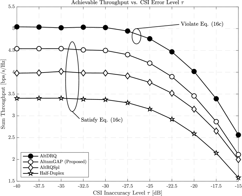
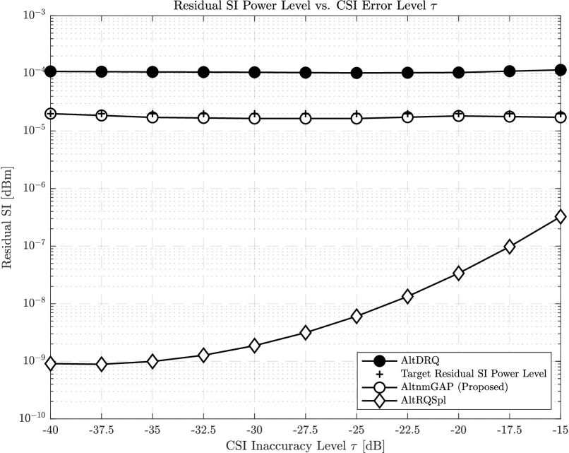
Figure 2: Achievable sum-throughput comparisons of the proposed method against the state-of-the-art SI cancellation methods as well as the conventional half-duplex as a function of the channel estimation accuracy level $\tau$ with a moderate hardware distortion level $\beta=-50$ dB.

Figure 3: Residual SI power levels after processing by the analog cancellation at the FD receiver for different methods ($i.e.,$ the proposed and state-of-the-arts) as a function of the channel estimation accuracy level $\tau$ with a moderate hardware distortion level $\beta=-50$ dB, where the target residual SI level is highlighted by the marker “plus”.

Figure 3 illustrates the achievable sum-throughput performance of the proposed ALTnmGAP method in comparison with the state-of-the-art methods [20, 23] as a function of the CSI accuracy parameter $\tau$ subject to moderate hardware impairment level $\beta=-50$ dB, where the performance corresponding to the half-duplex mode is also offered for the sake of comparison. As highlighted in the figure, it can be observed that the proposed method can achieve the maximum throughput among the methods satisfying the residual SI power level given in equation (18c), which can be confirmed in Figure 3. The residual SI power level after processing by the analog cancellation is shown in Figure 3 as a function of $\tau$, which clearly demonstrates the fact that the proposed method can suppress the residual SI at the receiver analog domain below the target over a wide range of CSI inaccuracy. Please note in the figure that the target SI residual level is denoted by the marker “plus” for the sake of readability. All in all, one may conclude that the proposed method can be seen as a compromise solution balancing the achievable throughput performance and the residual SI level requirement at the receiver analog domain so that the FD communications can enjoy the RF dynamic range at the receiver.

V Conclusion

This article studied a bidirectional in-band FD MIMO system subject to imperfect CSI, hardware distortion, and limited analog cancellation capability as well as the SI power requirement at the receiver analog domain such that the residual SI at the receiver analog domain may not pose saturation of the LNA. An optimization problem aiming at maximizing the sum SINR while satisfying the transmit power constraint and the residual SI power level requirement is formulated, proposing a new gradient projection based SI cancellation mechanism in conjunction with the concept of non-monotonicity. Simulation results demonstrated that the proposed method is a compromise solution to the latter problem, which balances the throughput performance and residual SI requirements.

References

- [1] D. Bharadia, E. McMilin, and S. Katti, “Full Duplex Radios,” in Proc. ACM SIGCOMM., Hong Kong, China, 12–16 Aug. 2013, pp. 375–386.
- [2] E. Everett, M. Duarte, C. Dick, and A. Sabharwal, “Empowering full-duplex wireless communication by exploiting directional diversity,” in Proc. Asilomar CSSC, Pacific Grove, CA, USA, Nov. 2011, pp. 2002–2006.
- [3] J. I. Choi, M. Jain, K. Srinivasan, P. Levis, and S. Katti, “Achieving single channel, full duplex wireless communication,” in Proc. MobiCom, New York, NY, USA, Sep. 20 - 24 2010, pp. 1–12.
- [4] M. Duarte and A. Sabharwal, “Full-Duplex Wireless Communications Using Off-the-Shelf Radios: Feasibility and First Results,” in Proc. Asilomar CSSC, Nov 2010, pp. 1558–1562.
- [5] M. Jain, J. I. Choi, T. M. Kim, D. Bharadia, S. Seth, K. Srinivasan, P. Levis, S. Katti, and P. Sinha, “Practical, real-time, full duplex wireless,” in Proc. ACM Mobicom, Las Vegas, USA, Sep. 2011, pp. 301–312.
- [6] D. W. Bliss, P. A. Parker, and A. R. Margetts, “Simultaneous transmission and reception for improved wireless network performance,” in Proc. IEEE WSSP, 2007.
- [7] B. Radunovic, D. Gunawardena, P. Key, A. Proutiere, N. Singh, V. Balan, and G. Dejean, “Rethinking indoor wireless mesh design: Low power, low frequency, full-duplex,” in Proc. WIMESH, 2010, pp. 1–6.
- [8] M. Vehkaperä, T. Riihonen, and R. Wichman, “Asymptotic analysis of full-duplex bidirectional MIMO link with transmitter noise,” in Proc. IEEE PIMRC, London, UK, Sep. 2013, pp. 1265–1270.
- [9] H. Iimori, G. Abreu, and G. C. Alexandropoulos, “Full-duplex transmission optimization for bi-directional MIMO links with QoS guarantees,” in Proc. IEEE GlobalSIP, Anaheim, USA, Nov. 2018, pp. 1–5.
- [10] B. Day, A. Margetts, D. Bliss, and P. Schniter, “Full-duplex bidirectional MIMO: Achievable rates under limited dynamic range,” IEEE Trans. Signal Process., vol. 60, no. 7, pp. 3702 – 3713, Jul 2012.
- [11] T. Riihonen, M. Vehkaperä, and R. Wichman, “Large-system analysis of rate regions in bidirectional full-duplex MIMO link: Suppression versus cancellation,” in Proc. IEEE CISS, Baltimore, USA, Mar. 2013, pp. 1–6.
- [12] N. M. Gowda and A. Sabharwal, “Jointnull: Combining reconfigurable analog cancellation with transmit beamforming for large-antenna full-duplex wireless,” IEEE Trans. Wireless Commun., vol. 17, no. 3, pp. 2094 – 2108, Mar. 2018.
- [13] D. Korpi, L. Anttila, and M. Valkama, “Reference receiver based digital self-interference cancellation in mimo full-duplex transceivers,” in Proc. IEEE GC Wkshps, vol. 1-7, Austin, TX, USA, 8-12 Dec 2014.
- [14] H. Iimori and G. Abreu, “Two-way full-duplex MIMO with hybrid TX-RX MSE minimization and interference cancellation,” in Proc. IEEE SPAWC, Kalamata, Greece, 25-28 Jun. 2018, pp. 1–6.
- [15] O. Taghizadeh and R. Mathar, “Interference mitigation via power optimization schemes for full-duplex networking,” in Proc. WSA, Ilmenau, Germany, 2015.
- [16] O. Taghizadeh, V. Radhakrishnan, A. C. Cirik, R. Mathar, and L. Lampe, “Hardware impairments aware transceiver design for bidirectional full-duplex MIMO OFDM systems,” IEEE Trans. Veh. Technol., vol. 67, no. 8, pp. 7450–7464, Aug. 2018.
- [17] M. S. Sim, M. Chung, D. Kim, J. Chung, D. K. Kim, and C.-B. Chae, “Nonlinear self-interference cancellation for full-duplex radios: From link-level and system-level performance perspectives,” IEEE Commun. Mag., vol. 55, no. 9, pp. 158–167, Jun. 2017.
- [18] A. C. Cirik, R. Wang, and Y. Hua, “Weighted-sum-rate maximization for bi-directional full-duplex MIMO systems,” in Proc. Asilomar Conf. Signals, Syst. Comput., Nov. 2013.
- [19] K. E. Kolodziej, J. G. McMichael, and B. T. Perry, “Multitap RF canceller for in-band full-duplex wireless communications,” IEEE Trans. Wireless Commun., vol. 15, no. 6, pp. 4321–4334, Jun. 2016.
- [20] G. C. Alexandropoulos and M. Duarte, “Joint design of multi-tap analog cancellation and digital beamforming for reduced complexity full duplex MIMO systems,” in Proc. IEEE ICC, Paris, France, 21–25 May 2017, pp. 1–7.
- [21] D. Liu, Y. Shen, S. Shao, Y. Tang, and Y. Gong, “On the analog self-interference cancellation for full-duplex communications with imperfect channel state information,” IEEE Access, vol. 5, pp. 9277–9290, May 2017.
- [22] A. T. Le, L. C. Tran, X. Huang, and Y. J. Guo, “Beam-based analog self-interference cancellation in full-duplex MIMO systems,” IEEE Trans. Wireless Commun., vol. 19, no. 4, pp. 2460–2471, Apr. 2020.
- [23] H. Iimori, G. T. F. de Abreu, and G. C. Alexandropoulos, “MIMO beamforming schemes for hybrid SIC FD radios with imperfect hardware and CSI,” IEEE Trans. Wireless Commun., vol. 18, no. 10, pp. 4816–4830, Oct. 2019.
- [24] H. Iimori, R.-A. Stoica, and G. T. F. de Abreu, “Constellation shaping for rate maximization in AWGN channels with non-linear distortion,” in Proc. IEEE CAMSAP, Curacao, Netherlands Antilles, 2017, pp. 1–5.
- [25] O. Taghizadeh, A. C. Cirik, and R. Mathar, “Hardware impairments aware transceiver design for full-duplex amplify-and-forward MIMO relaying,” IEEE Trans. Wireless Commun., vol. 17, no. 3, pp. 1644–1659, Mar. 2018.
- [26] H. Iimori and G. T. F. de Abreu, “Performance analysis of non-linear wireless communications in ultra dense networks,” in Proc. IEEE ICC, Kansas, USA, 2018, pp. 1–6.
- [27] L. Musavian, M. R. Nakhai, M. Dohler, and A. H. Aghvami, “Effect of channel uncertainty on the mutual information of MIMO fading channels,” IEEE Trans. Veh. Technol., vol. 56, no. 5, pp. 2798–2806, Sept. 2007.
- [28] C. Wang, E. K. S. Au, R. D. Murch, W. H. Mow, R. S. Cheng, and V. Lau, “On the performance of the MIMO zero-forcing receiver in the presence of channel estimation error,” IEEE Trans. Wireless Commun., vol. 6, no. 3, pp. 805–810, 2007.
- [29] M. Duarte, C. Dick, and A. Sabharwal, “Experiment-driven characterization of full-duplex wireless systems,” IEEE Trans. Wireless Commun., vol. 11, no. 12, pp. 4296–4307, Dec. 2012.
- [30] F. Negro, S. P. Shenoy, I. Ghauri, and D. T. M. Slock, “On the MIMO interference channel,” in Proc. Inf. Theory Appl. Workshop, San Diego, USA, 31 Jan.–5 Feb. 2010, pp. 1–9.
- [31] H. Li and Z. Lin, “Accelerated proximal gradient methods for nonconvex programming,” in Proc. NIPS, 2015, pp. 379–387.
- [32] Q. Yao, J. T. Kwok, F. Gao, W. Chen, and T.-Y. Liu, “Efficient inexact proximal gradient algorithm for nonconvex problems,” in Proc. IJCAI, 2017, pp. 3308–3314.
- [33] B. P. Day, A. R. Margetts, D. W. Bliss, and P. Schniter, “Full-duplex MIMO relaying: Achievable rates under limited dynamic range,” IEEE Journal on Selected Areas in Communications, vol. 30, no. 8, pp. 1541–1553, Sep. 2012.
- [34] H. Iimori, G. Abreu, and G. C. Alexandropoulos, “Full-duplex bi-directional MIMO under imperfect CSI and hardware impairments,” in Proc. IEEE WPNC, Bremen, Germany, 2018, pp. 1–6.
- [35] H. Shen, B. Li, M. Tao, and X. Wang, “MSE-based transceiver designs for the MIMO interference channel,” IEEE Trans. Wireless Commun., vol. 9, no. 11, pp. 3480–3489, Nov. 2010.
- [36] M. Grant and S. Boyd. (2017) CVX: Matlab software for disciplined convex programming. [Online]. Available: http://cvxr.com/cvx/
- [37] S. Diamond and S. Boyd, “CVXPY: A Python-embedded modeling language for convex optimization,” Journal of Machine Learning Research, vol. 17, no. 83, pp. 1–5, 2016.
- [38] M. Udell, K. Mohan, D. Zeng, J. Hong, S. Diamond, and S. Boyd, “Convex optimization in julia,” in Proc. HPTCDL, 2014.
- [39] E. D. Andersen and K. D. Andersen, “The MOSEK interior point optimizer for linear programming: An implementation of the homogeneous algorithm,” High Perform. Opt., vol. 33, pp. 197–232, 2000.
- [40] S. Adachi and Y. Nakatsukasa, “Eigenvalue-based algorithm and analysis for nonconvex QCQP with one constraint,” Math. Program., vol. 173, no. 1–2, pp. 79–116, Jan. 2019.