Constructing rigid-foldable generalized Miura-ori tessellations for curved surfaces

Abstract

Origami has shown the potential to approximate three-dimensional curved surfaces by folding through designed crease patterns on flat materials. The Miura-ori tessellation is a widely used pattern in engineering and tiles the plane when partially folded. Based on constrained optimization, this paper presents the construction of generalized Miura-ori patterns that can approximate three-dimensional parametric surfaces of varying curvatures while preserving the inherent properties of the standard Miura-ori, including developability, flat-foldability and rigid-foldability. An initial configuration is constructed by tiling the target surface with triangulated Miura-like unit cells and used as the initial guess for the optimization. For approximation of a single target surface, a portion of the vertexes on the one side is attached to the target surface; for fitting of two target surfaces, a portion of vertexes on the other side is also attached to the second target surface. The parametric coordinates are adopted as the unknown variables for the vertexes on the target surfaces whilst the Cartesian coordinates are the unknowns for the other vertexes. The constructed generalized Miura-ori tessellations can be rigidly folded from the flat state to the target state with a single degree of freedom.

1 Introduction

Origami has emerged as a technology to construct three-dimensional (3D) folded structures by folding a piece of flat material. The folded configurations that can be attained depend on the crease pattern which consists of mountain/valley creases and vertexes. Among the various crease patterns, the standard Miura-ori pattern is probably the most well-studied and widely used pattern in engineering. It was proposed for the packaging and deployment of large membranes in space [1, 2]; the pattern and its variants have found applications as the foldcores of sandwich structures [3, 4, 5, 6]. Recently, unique properties of origami structures, such as negative Poisson’s ratio and multi-stability, have been revealed by researchers and the Miura-ori tessellation has inspired the design of mechanical and acoustic metamaterials, see [7, 8, 9, 10] among others.

The standard Miura-ori tessellation is made up of a number of identical unit cells, or Miura cells, and each cell consists of four congruent parallelograms, see Fig.1(a), (b) and (c). Each interior vertex is of degree-4 with one pair of creases symmetric with respect to the other collinear pair. For stiff facets connected by soft creases, it would be much harder to bend the facets than to fold along the creases, thus the morphing of the origami structures can be described by the rigid origami model in which all the facets are assumed rigid and only folding along the creases are allowed. Treated as the rigid origami, the Miura-ori tessellation constitutes a mechanism which folds with a single degree of freedom (DOF) before all the facets collapse into the same plane. In all the partially folded states, the Miura-ori tessellation can only exhibit in-plane motion and tiles the plane. To approximate 3D curved surfaces, variations in the edge length and sector angles of the cells should be involved, see Fig.1(d) for an illustration of a generalized Miura cell. However, for a general quadrilateral mesh, rigid-foldability is nontrivial since the compatibility between all the rigid facets during the folding process can lead to an overconstrained mechanism [11, 12]. It has been shown by Tachi that standard Miura-ori pattern can be perturbed into general ones which satisfy the developability, flat-foldability and other constraints [11, 13]. The resulting generalized patterns can approximate some curved surfaces when partially folded. Most importantly, it has been proven that if an intermediate folded state exists for a quadrilateral mesh consisting of developable and flat-foldable vertexes, the pattern is rigid-foldable limited only by the avoidance of self-penetrations [11, 14]. Based on the findings, Tachi has developed the “Freeform origami” software which can modify the standard Miura-ori tessellation (and other tessellations) into some curved structure by interactively moving the vertexes and projecting the perturbation into the constraint space [15, 13]. However, it is difficult for the software to tackle inverse design problems since constraints regarding approximating target surfaces are not considered yet. By altering a single characteristic of the Miura-ori cell, Gattas et al. have investigated the parameterizations of first-level Miura-ori derivative patterns [16]. Lang and Howell proposed a method to construct rigid-foldable quadrilateral meshes based on the inherent relations between the sector and fold angles of flat-foldable vertexes [17]. Recently, Dieleman et al. developed a systematic approach by first identifying a number of rigid-foldable motifs as jigsaw puzzle pieces and then fitting them together to obtain large rigid-foldable crease patterns [12].

Several approaches have been developed for the design of cylindrical and axisymmetric origami structures [18, 19, 20, 21]. Due to the symmetry of the target cylindrical/axisymmetric surfaces, the crease patterns observe collinear creases which are parallelly (radially) spaced for the cylindrical (axisymmetric) cases. Though restrictive in the designed geometry, the approaches in the references [18, 19, 20, 21] can be used to design folded structures which fit two given target surfaces. Dudte et al. have proposed an optimization-based algorithm to find the intermediate folded form which approximates general curved surfaces [22]. In this algorithm, the target surface is first tiled with a Miura-like tessellation. To ensure the approximation, the four corner vertexes of each cell (vertexes 1, 3 ,7 and 9 of each cell shown in Fig.1(d)) are fixed as the initial guess whilst the positions of the other vertexes are searched by the optimization method to meet the constraints, including the planarity of all the quadrilaterals and the developability at all the interior vertexes. However, it was reported that the algorithm fails to find the folded form that satisfies the flat-foldability condition for general curved surfaces. Due to the aforementioned theorem by Tachi [11], the patterns constructed by Dudte et al. are not rigid-foldable, i.e., the quadrilateral facets will be bent along the diagonals when it is folded from the flat state to the target state. To approach the flat-foldability (and thus the rigid-foldability), the flat-foldability constraint is replaced by inequalities with auxiliary tolerance [22]. However, this remedy can only reduce the bending energy of the quadrilateral whilst the crease patterns consist of triangular facets during the folding process. While introducing diagonal creases enlarges the space of rigid-foldable configurations, extra efforts are required when folding the flat pattern into the target form due to the introduced DOFs and the complex interaction between the energy potential and the rigid origami [23]. The failure in satisfying the flat-foldability condition may be caused by the fact that all the four corner vertexes of each cell are fixed during the optimization which reduces the number of variables in the algorithm. In fact, the position of corner vertexes should also be rearranged to enlarge the searching space such that flat- and rigid-foldable crease pattern may be found for a curved target surface.

In this paper, based on the constrained optimization, we present the construction of generalized Miura-ori tessellation for 3D curved parametric surfaces which can be folded rigidly from the flat state to the target form with a single degree of freedom. The construction is based on the rigid origami model, which ngelects the deformation of facets and creases. The construction utilizes general quadrilateral mesh with developable and flat-foldable interior vertexes whilst the mountain and valley crease assignment is kept the same as that of the Miura-ori pattern. The target surface is first tiled with triangulated Miura-like cells and then the optimization method is used to enforce the constraints, including the planarity of all the quadrilaterals, developability and flat-foldability at all the interior vertexes. To ensure the fitting, a portion of vertexes on the one side is attached to the target surface; another portion of vertexes on the other side is also attached to the second target surface if a second target surface is to be approximated. For the attached vertexes, the parametric coordinates are adopted as the unknown variables whilst the Cartesian coordinates are the unknowns for the other vertexes. Several examples of fitting a single target surface and two target surfaces are considered to demonstrate the feasibility of the algorithm.

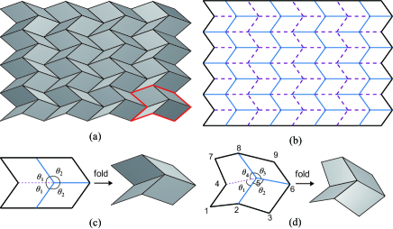
Figure 1: (a) The Miura-ori tessellation with 4$\times$4 unit cells in its partially folded state; (b) the associated crease pattern where the mountain and valley creases are indicated by solid and dashed lines, respectively; (c) a standard Miura cell in which $\theta_{i}$ are the sector angles between two creases; (d) the generalized Miura cell with four irregular quadrilaterals; the sector angles are required to satisfy $\theta_{1}+\theta_{2}+\theta_{3}+\theta_{4}=2\pi$ for developability and $\theta_{1}+\theta_{3}=\theta_{2}+\theta_{4}=\pi$ for flat-foldability at the central vertex.

2 Approximate a single target surface

2.1 Initial tessellation construction and the constraints

Fig.1(c) shows the standard Miura-ori cell made up of four congruent parallelograms. The interior vertex is of valence four with one valley crease and three mountain creases or vice versa. Besides, one pair of creases are symmetric with respect to the other collinear pair. The Miura tessellation is the repeating of the unit cells and tiles the plane in its partially folded states. To approximate curved surfaces, the edge length and sector angles of the cells should vary across the pattern while the basic rules of Miura pattern, including developability, flat-foldability and rigid-foldability, have to be fulfilled. A generalized Miura cell is illustrated in Fig.1(d) which consists of four quadrilaterals and the cell is developable and flat-foldable, i.e., the sector angles around the central vertex satisfy

$$\theta_{1}+\theta_{2}+\theta_{3}+\theta_{4}=2\pi\quad\text{and}\quad\theta_{1}+\theta_{3}=\theta_{2}+\theta_{4}=\pi$$ (1)

for developability and flat-foldability, respectively [11, 14].

As pointed out by Dudte et.al [22], the basic steps for constructing tessellations for curved surfaces based on optimization are: first, generate an initial Miura-like tessellation as an initial guess for the optimization algorithm which does not have to satisfy the constraints; then, enforce the constraints, including developability, flat-foldability and etc, by the constrained optimization with appropriate objective function. Similar ideas have also been adopted by Bhooshan to generate curved folding based on the dynamic relaxation framework [24].

For expository purposes, we consider the target surface $z=xy/2$ with $x,y\in[-1,1]$ as an example. The target surface can be expressed in the parametric form as $\textbf{X}(r,s)=\{r,s,rs/2\}$. Fig.2 shows the construction of the initial triangulated Miura-like tessellation:

$\bullet$ A base mesh is first generated by the $r=r_{i}$ and $s=s_{i}$ coordinate lines with $r_{i}=-1+(i-1)\Delta r$ and $s_{i}=-1+(i-1)\Delta s$ for $i=1,2,\cdots,9$ and $\Delta r=\Delta s=1/4$. In other words, the $r_{i}$- and $s_{i}$-coordinate lines are equispaced in the $r$- and $s$-coordinates, respectively.

$\bullet$ Then, the vertexes on the $s_{i}$-coordinate lines with $i=2,4,6$ and 8 are moved along the $r$-coordinate by $l_{p}=\Delta r$, see Fig.2(b).

$\bullet$ Finally, the vertexes on the $r_{i}$-coordinate line with $i=2,4,6$ and 8 are moved along the normal of the target surface by $l_{h}=1.8\Delta r$; the quadrilateral mesh is triangulated by connecting vertex-($r_{i},s_{j}$) with vertex-($r_{i-1},s_{j+1}$) for $j=1,3,5,7$ and vertex-($r_{i},s_{j}$) with vertex-($r_{i+1},s_{j+1}$) for $j=2,4,6,8$.

The vertexes of each quadrilateral are noncoplanar in general and a representative triangulated cell is shown in Fig.3(a). It should be remarked that the initial triangulated Miura-like tessellation is not unique. By changing $l_{p}$ and $l_{h}$ (comparable to $\Delta r$ in general), different initial tessellations can be constructed. Compared with the construction process in the reference [22], the current construction suits for a large class of parametric surfaces and avoids the process of merging vertexes shared by adjacent cells.

The triangulated Miura cell in Fig.3(a) can be specified by the coordinates of the 9 vertexes. The planarity of the quadrilateral facets are to be restored in the optimization process. For the quadrilateral 1-2-5-4, the planarity of the quadrilateral facet requires that the volume of the hexagon formed by the vectors $\overrightarrow{P_{1}P_{2}}$, $\overrightarrow{P_{1}P_{4}}$ and $\overrightarrow{P_{1}P_{5}}$ equals 0, i.e.,

$$(\textbf{X}_{2}-\textbf{X}_{1})\times(\textbf{X}_{4}-\textbf{X}_{1})\cdot(\textbf{X}_{5}-\textbf{X}_{1})=0$$ (2)

where $\overrightarrow{P_{i}P_{j}}$ is the vector from vertex-$i$ to vertex-$j$ and $\textbf{X}_{i}$ is the Cartesian coordinate for the vertex-$i$. The planarity for the other quadrilaterals can be expressed analogously. Due to the triangulation, all the inner vertexes are of degree-6, see Fig.2(c). In Fig.3(a), the sector angles are denoted anticlockwise as $\alpha_{1}$ through $\alpha_{6}$ around the central vertex-5. The developability condition at vertex-5 is

$$\sum_{i=1}^{6}\alpha_{i}=2\pi\ .$$ (3)

When the coplanarity of the quadrilaterals 2-3-6-5 and 5-6-9-8 are restored, the diagonal lines 3-5 and 5-9 becomes redundant and the vertex-5 reduces to degree-4 vertex. In the optimization process, the flat-foldability condition at vertex-5 is

$$\alpha_{1}+\alpha_{4}+\alpha_{5}=\pi\ .$$ (4)

It is clear that the identity, $\alpha_{2}+\alpha_{3}+\alpha_{6}=\pi$, holds if Eq.(3) and Eq.(4) are satisfied. Considering the orientation of the quadrilateral facets and triangulation, the numbering of the sector angles in Fig.3(a) can be used for vertexes on the $s_{i}$-coordinate lines with $i=2,4,6,8$ while the numbering shown in Fig.3(b) should be adopted for the vertexes on the the $s_{i}$-coordinate lines with $i=1,3,5,7$ such that Eq.(4) is consistent for all interior vertexes. To facilitate the optimization algorithm, the derivatives of the constraints in Eq.(2), (3) and (4) with respect to the variables are supplied in the Appendix A. The triangulated Miura-like cell will turn into a generalized Miura cell if the constraints on quadrilateral facet planarity, developability and flat-foldability are satisfied simultaneously.

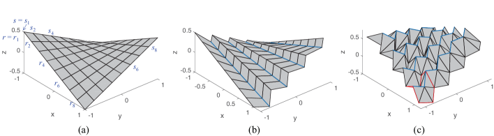
Figure 2: Generation of the initial 4$\times$4 triangulated Miura-like tessellation for the target surface $z=xy/2$, i.e., $\textbf{X}(r,s)=\{r,s,rs/2\}$: (a) the base mesh formed by the parametric lines $r=r_{i}$ and $s=s_{i}$ for $i=1,2,\cdots,9$; the $r_{i}$-coordinate lines are equispaced in the parametric coordinate $(\Delta r=2/8=1/4)$ and so are the $s_{i}$-coordinate lines; (b) the vertexes on the $s_{i}$-coordinate lines ($j=2,4,6,8$) are moved along the $r$-coordinate by $\Delta r$; (c) the vertexes on the $r_{i}$-coordinate line ($i=2,4,6,8$) are moved along the normal of the target surface by $1.8\Delta r$; triangulate the quadrilateral mesh by connecting vertex-($r_{i},s_{j}$) with vertex-($r_{i-1},s_{j+1}$) for $j=1,3,5,7$ and vertex-($r_{i},s_{j}$) with vertex-($r_{i+1},s_{j+1}$) for $j=2,4,6,8$.

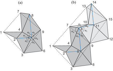
Figure 3: (a) A representative cell: $\alpha_{1}$ through $\alpha_{6}$ are the sector angles and the dashed lines indicate the auxiliary cell contour edges; (b) two adjacent cells. Due to the orientation of the quadrilateral facets and triangulation, the numbering of the sector angles for interior vertexes on the $s_{i}$-dinate lines with $i$ being even and odd follow that around vertex-5 in (a) and vertex-8 in (b), respectively.

2.2 The variables and objective function

To enforce a close approximation to the target surface, a portion of the vertexes is attached to the target surface. For the cell in Fig.3(a), it is most likely that the vertexes in the set {1,4,7,3,6,9} reside on the one side while vertexes in {2,5,8} on the other. Here, the corner vertexes of each cell, i.e., vertexes {1,7,3,9} in Fig.3(a), are chosen to be attached to the target surface. The attached vertexes are allowed to slide on the target surface. For the attached vertex-$j$, it is natural to use their Cartesian coordinates $\textbf{X}^{j}=\{x^{j},y^{j},z^{j}\}$ as the unknown variables while enforcing the attachment by satisfying the equation of the target surface, for example in the form of $z=f(x,y)$. This approach is still feasible when the target surface has explicit expression regarding $x$, $y$ and $z$ coordinates. However, for many parametric surfaces, it would be difficult to derive such a form and numerical root finding and derivative calculations are required. Instead, we adopt the parametric coordinates {$r^{j},s^{j}$} as the unknown variables for the attached vertex-$j$, i.e., $\textbf{X}^{j}=\{x(r^{j},s^{j}),y(r^{j},s^{j}),z(r^{j},s^{j})\}$, thus the vertex-$j$ naturally resides on the target surface. Aside from the attached vertexes, the Cartesian coordinates are adopted as the unknown variables for the other vertexes.

With the triangulated Miura-like tessellation as an initial guess, the optimization algorithm is utilized to adjust the vertex positions such that the constraints are fulfilled while minimizing appropriate objective function. Let $N$ be the set of all the vertexes; $E_{A}$ is set of auxiliary cell contour edges for all the triangulated Miura cells, see the dashed lines in Fig.3; $E$ be the set of all the edges and the total number of edges is $n_{E}$. Assuming that the initial triangulated Miura-like tessellation is a reasonable guess, the following objective function is suggested

$$f=\sum_{i\in E\bigcup E_{A}}(\frac{L^{i}}{L_{0}^{i}}-1)^{2}+\sum_{j\in N}\frac{1}{(L_{c})^{2}}(\textbf{X}^{j}-\textbf{X}_{0}^{j})^{2}$$ (5)

where $L^{i}$ is the edge length of the current configuration whilst $L_{0}^{i}$ is the counterpart of the initial guess; $L_{c}=\sum_{i\in E}L_{0}^{i}/n_{E}$ is the characteristic length; $\textbf{X}^{j}=\{x^{j},y^{j},z^{j}\}$ is the coordinate for the vertex-$j$ of the current configuration whilst $\textbf{X}_{0}^{j}$ is the counterpart of the initial guess. Furthermore, the parametric coordinates {$r^{j},s^{j}$} are the unknowns for the attached vertexes, i.e., $\textbf{X}^{j}=\{x(r^{j},s^{j}),y(r^{j},s^{j}),z(r^{j},s^{j})\}$, whilst the Cartesian coordinates $\{x^{j},y^{j},z^{j}\}$ are the variables for the other vertexes. The first term on the left hand of Eq.(5) is to preserve the relative distance between the vertexes such that no crease or boundary edge degenerates. The second term is to ensure that the vertexes are as close as possible to the initial guess, which also prevents the entire tessellation from sliding on the target surface. Both terms are dimensionless such that the objective function is scale independant.

For the tessellation with $m\times n$ triangulated Miura-like cells, there are $2m\times 2n$ quadrilaterals and each quadrilateral brings in one planarity constraint, see Eq.(2). Besides, there are $(2m-1)\times(2n-1)$ interior vertexes and, at each inner vertex, Eq.(3) and Eq.(4) should be satisfied for the local constraints on developability and flat-foldability. Thus, the total number of constraints is

$$N_{c}=4mn+2(2m-1)(2n-1)=12mn-4m-4n+2\ .$$ (6)

It is clear that the total number of vertexes is $(2m+1)(2n+1)$. As the four corner vertexes of each cell are chosen for the attachment, there are $(m+1)\times(n+1)$ vertexes with their parametric coordinates as the unknowns and each parametric vertex owns 2 variables. The total number of unknown variables and the excess DOFs are, respectively,

$$\begin{array}[]{c}N_{f}^{s}=3(2m+1)(2n+1)-(m+1)(n+1)=11mn+5m+5n+2\\ \text{and }N_{f}^{s}-N_{c}=-mn+9(m+n)\text{ .}\end{array}$$ (7)

When $N_{f}^{s}<N_{c}$, i.e., there are more constraints than variables, the optimization algorithm generally fails to find a generalized Miura-ori tessellation if there were no sufficient redundancy among the constraints. For the case of $m=n$, it is required that $m\leq 18$ to ensure that $N_{f}^{s}\geq N_{c}$.

The objective function in Eq.(5) together with the constraints in Eq.(2), (3) and (4) can be solved by standard optimization routines. Here, we adopt the interior-point method implemented in the fmincon routine of MATLAB. To facilitate the solution, the derivatives of the objective and constraint functions with respective to (w.r.t) the variables should be provided for fmincon and are discussed in the Appendix A.

For the construction of generalized Miura-ori tessellation with 4$\times$4 cells for $z=xy/2$, the fmincon converges in 93 iterations and the constraints are satisfied to the machine accuracy. The converged configuration is shown in Fig.4. It has been proved by Tachi that if there exist a partially folded form of the quadrilateral mesh with interior developable and flat-foldable vertexes, then the quadrilateral mesh is rigid-foldable limited only by the penetration avoidance (see Theorem 2 in the reference [11]). Thus, the origami is rigid-foldable with a single DOF. The crease pattern is given in Fig.4(b) in which the vertexes indicated by the blue dot are exactly on the target surface in the folded form shown in Fig.4(a). Since the origami constitutes a single DOF mechanism, the folded state can be characterized by any one of the dihedral angles between two adjacent facets. Here, as indicated in Fig.4(a), the dihedral angle $\gamma$ at the red crease is chosen which equals approximately 87.4^∘ for the target state. Following the procedures in Section 4 and Appendix A of the reference [17], the dihedral angles at all the interior creases and thus the 3D folded form can be obtained for given $\gamma$. It is checked that no penetration occurs between the facets, see Appendix B for detailed discussions. Several snapshots during the folding process are shown in Fig.5.

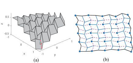
Figure 4: (a) The converged result of the 4$\times$4 Miura-ori tessellation for the target surface $z=xy/2$ and $\gamma$ ($\approx 87.4^{\circ}$) is the dihedral angle at the crease; (b) the crease pattern in which the solid dots are the vertexes attached to the target surface when the pattern is rigidly folded to the target state.

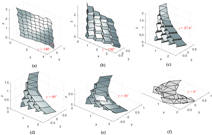
Figure 5: The snapshots for the folded form specified by the dihedral angle $\gamma$. (a) is the flat state; (c) is the same configuration as that in Fig.4(a) under a different view angle; (f) is the fully folded state with all facets being coplanar.

2.3 Further design examples

This subsection considers several examples to further illustrate the design algorithm which is implemented in MATLAB. The code is executed on a desktop with Intel(R) Core(TM) i7-6700 (8 cores, 3.41Gz). The details of the design cases are summarized in Table 1. The most time consuming part of the whole construction is to solve the optimization problem by the interior-point method of fmincon. As a rough reference of computational efficiency, the number of iterations and computational time (only the solution time of the fmincon routine) are listed. Besides, it is checked that the constraints including quadrilateral facet planarity, developability and flat-foldability at the interior vertexes are fulfilled to machine accuracy (of order less than $10^{-13}$). From the Table 1, it takes more iterations to search the solution for the sphere case. The converged folded forms, the crease pattern and the fully folded state are, respectively, shown in the first, second and third columns of Fig.6. It can be seen that the crease patterns for the cases (a), (c) and (d) are roughly symmetric with respect to the middle horizontal line.

Table 1: Summary of the design examples for single target surface (a) cylinder: $x^{2}+y^{2}=1$, (b) hyperbolic paraboloid: $z=xy$, (c) sphere: $x^{2}+y^{2}+z^{2}=1$ and (d) hyperboloid: $x^{2}+y^{2}-z^{2}=1$.

cases Target surface $\{x,y,z\}$ Cells Iterations Time(sec) (a) $\{\cos(r),\sin(r),s\}$ 8$\times$4 161 33.3 (b) $\{r,s,rs\}$ 8$\times$8 148 145.2 (c) $\{\cos(s)\cos(r),\cos(s)\sin(r),\sin(s)\}$ 8$\times$9 262 403.6 (d) $\{\sqrt{1+s^{2}}\cos(r),\sqrt{1+s^{2}}\sin(r),s\}$ 8$\times$9 151 192.8

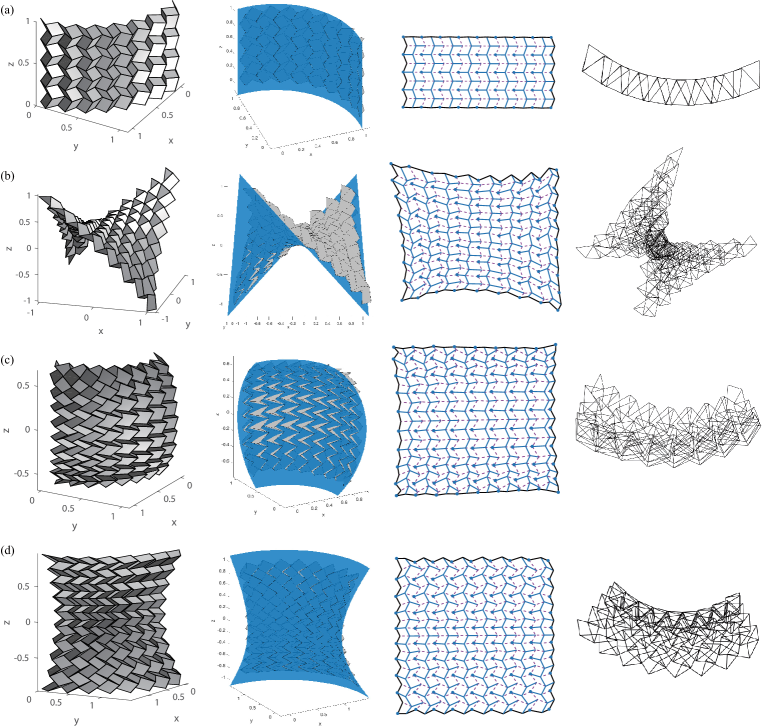
Figure 6: Examples of approximating a single target surface: the folded forms (first and second columns), the crease patterns (third column) and the fully folded state (fourth column), details are listed in Table 1. For figures in the second column, the target surface is also shown. For each case, the solid dots in the crease pattern in the third column are on the target surface when the pattern is folded to the state shown in the second column.

3 Fit two target surfaces

3.1 Construction process

It is of practical interest that the origami, when partially folded, the vertexes on each side approximate different given surfaces. Without losing generality, the two surfaces are denoted as lower surface $\textbf{X}_{l}$ and upper surface $\textbf{X}_{u}$. The construction of the initial triangulated Miura-like tessellation follows similar procedure as that for the single target surface. For clarity, the case with $\textbf{X}_{l}=\{r,s,0\}$ and $\textbf{X}_{u}=\{r,s,(1+rs)/2\}$ is considered as an example. Fig.7(a) shows the base mesh generated on the lower surface $\textbf{X}_{l}$ by the $r$- and $s$-coordinate lines. The $r_{i}$-coordinate lines are equispaced in the parametric coordinate $(\Delta r=1/4)$ and so are the $s$-coordinate lines. The vertexes on the $s_{2i}$-coordinate lines ($i=1,2,3$ and 4) are then moved along the $r$-coordinate by $\Delta r$ to form the mesh shown in Fig.7(b). After that, the vertexes on the $r_{2i}$-coordinate lines with $i=1,2,3$ and 4 are moved to the upper target surface $\textbf{X}_{u}$ by changing the $z$-coordinate of each vertex to $(1+rs)/2$. The vertexes on the blue lines in Fig.7(c) are then on the upper target surface. The initial construction does not constitute a generalized Miura-ori tessellation as the constraints, i.e., quadrilateral facet planarity, developability and flat-foldability, are not fulfilled in general.

For the cell shown in Fig.3(a), the vertexes {1, 3, 7, 9} are attached to the lower surface whilst the vertex-5 is attached to the upper surface. For the attached vertexes, the associated parametric coordinates are the variables whilst the other vertexes own the Cartesian coordinates as the variables. The construction then resorts to the optimization algorithm (the fmincon routine in the current implementation) to enforce the constraints on quadrilateral facet planarity, developability and flat-foldability, i.e., Eq.(2), (3) and (4), respectively. For the case in Fig.7, the fmincon convergences in 85 iterations and the final configuration is shown in Fig.7(d) and (e). The crease pattern is shown in Fig.7(f). It is checked that the constraints are fulfilled to machine accuracy. Due to the Theorem 2 of the reference [11], the pattern is rigid-foldable and no penetration is observed before it is fully folded.

For a tessellation with $m\times n$ cells, the number of constraints are the same as Eq.(6). Compared to the single target surface case, the central vertex (vertex-5 in Fig.) of each cell is also attached to the upper surface, thus the total number of variables and the number of excess DOFs are

$$N_{f}^{d}=N_{f}^{s}-mn=10mn+5m+5n+2\quad\text{and}\quad N_{f}^{d}-N_{c}=-2mn+9(m+n)$$ (8)

respectively. For the case with $m=n$, it is required that $m\leq 9$ to ensure that $N_{f}^{s}\geq N_{c}$, i.e., the number of variables should be larger than that of the constraints. When $N_{f}^{s}<N_{c}$, the optimization algorithm generally fails to find a generalized Miura-ori tessellation.

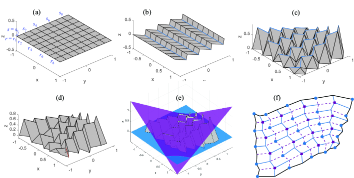
Figure 7: For the two target surfaces $\textbf{X}_{l}=\{r,s,0\}$ and $\textbf{X}_{u}=\{r,s,(1+rs)/2\}$, (a), (b) and (c) illustrate the generation of the initial 4$\times$4 triangulated Miura-like tessellation whilst (d), (e) and (f) are the converged results: (a) the base mesh formed on $\textbf{X}_{l}$ by the parametric coordinate lines $r=r_{i}$ and $s=s_{i}$ for $i=1,2,\cdots,9$; the $r_{i}$-coordinate lines are equispaced in the parametric coordinate $(\Delta r=1/4)$ and so are the $s$-coordinate lines; (b) the vertexes on the $s_{2i}$-coordinate lines ($i=1,2,3,4$) are moved along the $r$-coordinate by $\Delta r$; (c) the vertexes on the $r_{2i}$-coordinate line ($i=1,2,3,4$) are moved up to the upper target surface; (d) the converged folded form and $\gamma$ ($\approx 77.1^{\circ}$) is the dihedral angle at the crease; (e) the folded form with the upper and lower target surfaces shown; (f) the crease pattern where the solid dots and squares are the vertexes attached to the lower and upper target surfaces, respectively.

3.2 Further design examples

This subsection considers several examples to further illustrate the design algorithm for approximating two target surfaces. The details of the implementation are the same as those in section 2.3. Table 2 summarizes the parameters for each cases. The resulting folded forms are shown in the first and second columns of Fig.8 whilst the crease patterns and the fully folded states are listed in the third and fourth columns, respectively.

Table 2: Summary of the design examples for approximating two target surfaces.

cases Lower target surface $\textbf{X}_{l}$ Upper target surface $\textbf{X}_{u}$ Cells Iterations Time(sec) (a) $\{r,s,-(r^{2}+s^{2})/5\}$ $\{r,s,-(r^{2}+s^{2})/5+1/2\}$ 4$\times$8 129 28.1 (b) $\{r,s,rs/4\}$ $\{r,s,rs/4+1/2\}$ 4$\times$8 162 37.6 (c) $\{\cos(s)\cos(r),\cos(s)\sin(r),\sin(s)\}$ $1.2\times\{\cos(s)\cos(r),\cos(s)\sin(r),\sin(s)\}$ 8$\times$4 110 40.8 (d) $\{\sqrt{1+s^{2}}\cos(r),\sqrt{1+s^{2}}\sin(r),s\}$ $\{\sqrt{2+s^{2}}\cos(r),\sqrt{2+s^{2}}\sin(r),s\}$ 4$\times$8 84 24.3

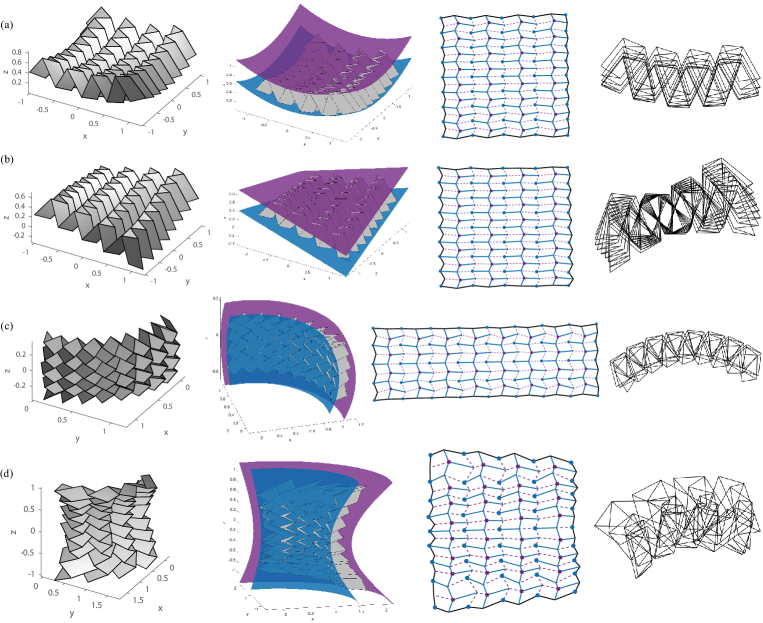
Figure 8: Examples of approximating two target surfaces: the folded forms (first and second columns), the crease patterns (third column) and the fully folded state (fourth column), details are listed in Table 2. For figures in the second column, the lower and upper target surfaces are also shown. The solid dots and squares in the crease patterns are attached to the lower and upper surfaces, respectively.

3.3 Airfoil example

In this section, the lower and upper target surfaces are adopted from the NACA-2412 airfoil, see Fig.9. The parametric equations are given in the Appendix C. It is difficult to find explicit expressions regarding $\{x,y,z$} for the target surfaces. Thus, if the Cartesian coordinates of all the vertexes were chosen as the variables, it would be inconvenient to enforce the attachment of vertexes to the target surfaces through additional constraints regarding the variables $\{x,y,z$}. Using the parametric coordinates for the pertinent vertexes as the variables avoids this difficulty. Besides, the vertexes at the bottom and tip ends remain respectively in the $y=0$ and $y=2$ planes during the optimization which is enforced by adding linear constraints on the pertinent $y$-coordinate ($y=0$ for the bottom end and $y=2$ for the top end) or $s$-coordinate for vertexes with parametric variables ($s=0$ for the bottom end and $s=1$ for the top end).

First, a tessellation with 3$\times$12 cells is considered. Similar to the previous examples, the vertexes {1,3,7,9} and {5} of each cell are, respectively, attached to the lower and upper target surfaces. The resulting folded form is shown in Fig.10(a) and (b) with different view angles. Fig.10(c) shows the crease pattern in which the blue dots and purple squares are on the lower and upper surfaces when the pattern is folded to the target state. From Fig.10(a) and (b), it can be seen that a large number of vertexes (51 out of the 175) extrude out of the target surface. By observing the relative position of the vertexes on each zigzag line in Fig.10(b) and (c), the vertexes attached to the lower and upper target surfaces are re-selected which is shown by the blue dots and purple squares in Fig.10(f). From the same initial triangulated Miura-ori tessellation, the optimization algorithm yields the improved folded form, see Fig.10(d) and (e), and few vertexes (10 out of the 175) are outside of the region. Next, the tessellation with 4$\times$16 cells is considered. When the vertexes {1,3,7,9} and {5} of each cell are, respectively, attached to the lower and upper target surfaces, the algorithm fails to find a valid folded form. This failure may indicate that too many vertexes are attached to the target surfaces. To enlarge the solution space, fewer interior vertexes are attached to the target surfaces, see Fig.11(c). The folded form is shown in Fig.11(a) and (b).

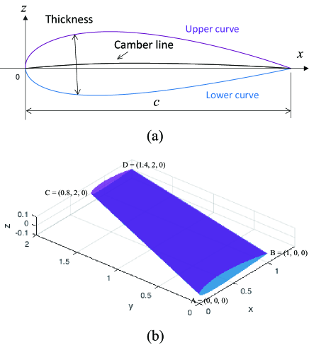
Figure 9: (a) The cross section of the NACA four-digit airfoil [25]; (b) the lower and upper surfaces of the airfoil constructed from the cross sections at the bottom ($y=0$) and tip ($y=2$) end; A, B, C and D indicate the corner points.

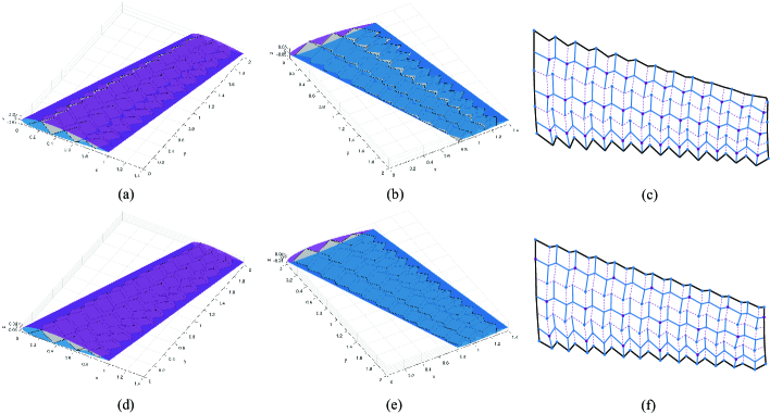
Figure 10: The resulting designs by attaching different sets of vertexes to the target surfaces: the attached vertexes are indicated by dots (on lower surface) and squares (on upper surface) in the crease patterns in (c) and (f); (a) and (b) are the folded form for (c) whilst (d) and (e) are the counterparts for (f).

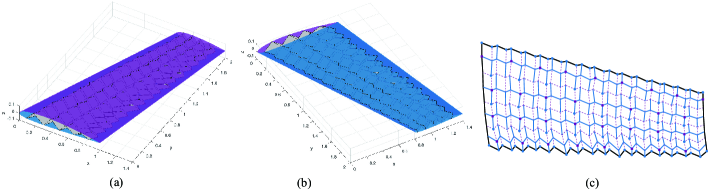
Figure 11: The designs with 4$\times$16 cells: (a) and (b) are the folded form; (c) shows the crease pattern where the solid dots and squares are attached to the lower and upper target surfaces, respectively.

4 Conclusion

This paper has presented the construction of rigid-foldable generalized Miura-ori tessellations which can approximate curved parametric surfaces based on constrained optimization. The algorithm is capable to approximate a single or double target surfaces by attaching portions of vertexes to the pertinent target surfaces. All the inherent properties of standard Miura-ori fold, including quadrilateral facet planarity, developability and flat-foldability, are enforced through optimization. To enlarge the searching space, the attached vertexes are allowed to slide on the target surface through using their parametric coordinates as the variables. Tessellations for target surfaces with varying curvatures in both directions have been constructed which are rigid-foldable with a single degree of freedom.

A limitation of the current algorithm is that the number of attached vertexes is restricted such that the optimization problem is not over-constrained, see Eq.(7) and (8) for the approximation of single and double target surfaces, respectively. While a re-selecting strategy is suggested and illustrated in Section 3.3, vertexes to be attached to the target surfaces are still chosen empirically in both layout and number. Neverthless, the present algorithm can be an efficient tool to generate small, rigid-foldable, curved patches which may be used as building blocks to piece up larger rigid-folable crease patterns [14, 17, 12].

The authors would like to thank Dr. Shuo Feng for insightful discussions. This work is supported by the National Natural Science Foundation of China (Nos. 11272303, 11072230, and 11802107), the Fundamental Research Funds for the Central Universities of China (Nos. WK2480000001 and WK2090050040) and the support of Entrepreneurship and Innovation Doctor Program in Jiangsu Province.

Appendix A Derivatives of the objective and constraint functions

This appendix discusses the derivatives of the objective and constraint functions which should be provided to enhance the efficiency of the optimization solver. The derivatives with respective to (w.r.t) the Cartesian coordinates are considered first. The derivatives of the objective function in Eq.(5) and the quadrilateral facet planarity constraint in Eq.(2) w.r.t to the Cartesian coordinates can be ready obtained and are not detailed here. For an interior vertex, the developability and flat-foldability constraints are the sum of the pertinent sector angles around the vertex. Each sector angle is determined by the three vertexes of the triangle where it resides. For a typical triangle shown in Fig.12, the sector angle $\alpha$ is given by

$$\alpha=\arccos(\frac{(\textbf{X}_{2}-\textbf{X}_{1})\cdot(\textbf{X}_{3}-\textbf{X}_{1})}{\left\|\textbf{X}_{2}-\textbf{X}_{1}\right\|\left\|\textbf{X}_{3}-\textbf{X}_{1}\right\|})\ .$$ (9)

The derivatives of $\alpha$ w.r.t the vertex coordinates are (also see Eqs.(12), (13) and (14) of reference [15])

$$\frac{\partial\alpha}{\partial\textbf{X}_{2}}=-\frac{\textbf{n}\times(\textbf{X}_{2}-\textbf{X}_{1})}{\left\|\textbf{X}_{2}-\textbf{X}_{1}\right\|^{2}}$$ (10a)

$$\frac{\partial\alpha}{\partial\textbf{X}_{3}}=\frac{\textbf{n}\times(\textbf{X}_{3}-\textbf{X}_{1})}{\left\|\textbf{X}_{3}-\textbf{X}_{1}\right\|^{2}}$$ (10b)

$$\frac{\partial\alpha}{\partial\textbf{X}_{1}}=-\frac{\partial\alpha}{\partial\textbf{X}_{2}}-\frac{\partial\alpha}{\partial\textbf{X}_{3}}$$ (10c)

where $\textbf{n}=\frac{(\textbf{X}_{2}-\textbf{X}_{1})\times(\textbf{X}_{3}-\textbf{X}_{1})}{\left\|(\textbf{X}_{2}-\textbf{X}_{1})\times(\textbf{X}_{3}-\textbf{X}_{1})\right\|}$ is the unit normal of the triangle. Referring to the unit cell in Fig.3, the derivatives of the developability and flat-foldability constraints can then be obtained by adding the contributions from the sector angles around the central vertex. The derivatives w.r.t the parametric coordinates are obtained by the chain rule. For instance, assume that the vertex-1 of the triangle in Fig.12 is attached to the target surface and its unknown variables are $\{r_{1},s_{1}\}$, then the derivatives of the sector angle w.r.t the parametric coordinates are

$$\frac{\partial\alpha}{\partial r_{1}}=\frac{\partial\alpha}{\partial\textbf{X}_{1}}\cdot\frac{\partial\textbf{X}_{1}}{\partial r_{1}}\quad\text{and}\quad\frac{\partial\alpha}{\partial s_{1}}=\frac{\partial\alpha}{\partial\textbf{X}_{1}}\cdot\frac{\partial\textbf{X}_{1}}{\partial s_{1}}\ .$$ (11)

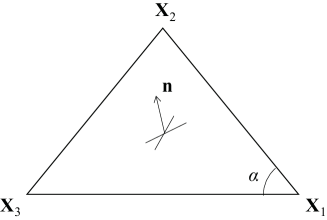
Figure 12: A typical triangle and n is its unit normal.

Appendix B Check of self-intersection

Thanks to the Theorem 2 of the reference [11], the crease pattern is rigid-foldable if an intermediate folded form exists for the quadrilateral mesh consisting of developable and flat-foldable vertexes. Nevertheless, the physically valid folded form of the crease pattern is limited by self-intersection. For the generalized Miura-ori pattern considered here, it is obvious that no self-intersection will be observed when the crease pattern is folded only by a small amount. As the folded form is of single degree-of-freedom (specified by the characteristic fold angle $\gamma$) and the shape morphing is smooth, contacts between the facets will happen when $\gamma$ reaches a certain critical value. After the converged design has been obtained for each case, we can view the three-dimensional folded form for given $\gamma$ and visually check whether global penetration occurs. For instance, for the case of $z=xy/2$ in Section 2.1 and 2.2, the folded form with $\gamma=0.1^{\circ}$ is plotted in Fig.13. There is no penetration even for this almost fully folded state.

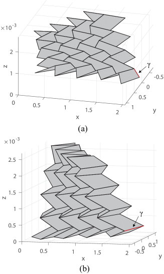
Figure 13: The folded form for the design resulf of $z=xy/2$ with $\gamma=0.1^{\circ}$: (a) and (b) are the folded form with different view angles. $\gamma$ is the dihedral angle at the crease indicated by the arrow. The scale of $z$-axis is much smaller than the others for better view.

Appendix C Lower and upper surfaces of the airfoil

Fig.9(a) shows the cross section of the NACA four-digit series airfoil in which $c$ is the airfoil chord. Introducing the parametric coordinate $r=x/c$, the camber line and the thickness distribution are, respectively, [25]

$$y_{c}(r)=\begin{cases}\begin{array}[]{c}\frac{\varepsilon cr}{p^{2}}(2p-r)\\ \frac{\varepsilon c(1-r)}{(1-p)^{2}}(1+r-2p)\end{array}&\begin{array}[]{c}0\leq r<p\\ p<r\leq 1\end{array}\end{cases}\quad\text{and}$$ (12a)

$$y_{t}(r)=10\tau c\left[0.2969\sqrt{r}-0.126r-0.3537r^{2}+0.2843r^{3}-0.1015r^{4}\right]$$ (12b)

in which $\varepsilon$, $p$ and $\tau$ are parameters. For the NACA-2412 airfoil considered in the example, the parameters are $\varepsilon=0.02,p=0.4$ and $\tau=0.12$. The lower and upper curves of the cross section are respectively

$$\left\{\begin{array}[]{c}x_{L}(c,r)\\ z_{L}(c,r)\end{array}\right\}=\left\{\begin{array}[]{c}c\times r+\frac{1}{2}y_{t}(r)\sin(\theta)\\ y_{c}-\frac{1}{2}y_{t}(r)\cos(\theta)\end{array}\right\}$$ (13)

and

$$\left\{\begin{array}[]{c}x_{U}(c,r)\\ z_{U}(c,r)\end{array}\right\}=\left\{\begin{array}[]{c}c\times r-\frac{1}{2}y_{t}(r)\sin(\theta)\\ y_{c}+\frac{1}{2}y_{t}(r)\cos(\theta)\end{array}\right\}$$ (14)

where

$$\theta=\arctan(\frac{dy_{c}}{dx})=\begin{cases}\begin{array}[]{c}\frac{2\varepsilon(p-r)}{p^{2}}\\ \frac{2\varepsilon(p-r)}{(1-p)^{2}}\end{array}&\begin{array}[]{c}0\leq r<p\\ p<r\leq 1\end{array}\end{cases}\ .$$

The cross sections at the bottom ($y=0$) and tip ($y=2$) ends are prescribed with the chord $c=1$ and $c=0.6$, respectively, see Fig.9(b). The lower curves of the cross sections at the bottom and tip ends are respectively

$$\textbf{X}_{L}^{b}=\left\{\begin{array}[]{c}x_{L}(1,r)\\ 0\\ z_{L}(1,r)\end{array}\right\}\quad\text{and}\quad\textbf{X}_{L}^{t}=\left\{\begin{array}[]{c}0.8+x_{L}(0.6,r)\\ 2\\ z_{L}(0.6,r)\end{array}\right\}\ .$$ (15)

The lower surface of the airfoil is a ruled surface which is given by

$$\textbf{X}_{L}(r,s)=(1-s)\textbf{X}_{L}^{b}+s\textbf{X}_{L}^{t}$$ (16)

The upper surface of the airfoil is defined in a similar way, i.e.,

$$\textbf{X}_{U}(r,s)=(1-s)\textbf{X}_{U}^{b}+s\textbf{X}_{U}^{t}$$ (17)

where

$$\textbf{X}_{U}^{b}=\left\{\begin{array}[]{c}x_{U}(1,r)\\ 0\\ z_{U}(1,r)\end{array}\right\}\quad\text{and}\quad\textbf{X}_{U}^{t}=\left\{\begin{array}[]{c}0.8+x_{U}(0.6,r)\\ 2\\ z_{U}(0.6,r)\end{array}\right\}\ .$$ (18)

are the upper cross-sectional curves at the bottom and top ends, respectively.

No algorithms.

References

- [1] Miura, K., 1970. “Proposition of pseudo-cylindrical concave polyhedral shells”. In Proceedings of IASS Symposium on Folded Plates and Prismatic Structures.
- [2] Miura, K., 1985. “Method of packaging and deployment of large membranes in space”. title The Institute of Space and Astronautical Science report, 618, p. 1.
- [3] Miura, K., 1972. “Zeta-core sandwich-its concept and realization”. title ISAS report/Institute of Space and Aeronautical Science, University of Tokyo, 37(6), p. 137.
- [4] Klett, Y., and Drechsler, K., 2011. “Designing technical tessellations”. In Origami 5: Fifth International Meeting of Origami Science, Mathematics, and Education, Taylor & Francis Group, Singapore, pp. 305–322.
- [5] Heimbs, S., 2013. “Foldcore sandwich structures and their impact behaviour: an overview”. In Dynamic failure of composite and sandwich structures. Springer, pp. 491–544.
- [6] Ma, J., Song, J., and Chen, Y., 2018. “An origami-inspired structure with graded stiffness”. International Journal of Mechanical Sciences, 136, pp. 134–142.
- [7] Wei, Z. Y., Guo, Z. V., Dudte, L., Liang, H. Y., and Mahadevan, L., 2013. “Geometric mechanics of periodic pleated origami”. Physical review letters, 110(21), p. 215501.
- [8] Schenk, M., and Guest, S. D., 2013. “Geometry of miura-folded metamaterials”. Proceedings of the National Academy of Sciences, 110(9), pp. 3276–3281.
- [9] Silverberg, J. L., Evans, A. A., McLeod, L., Hayward, R. C., Hull, T., Santangelo, C. D., and Cohen, I., 2014. “Using origami design principles to fold reprogrammable mechanical metamaterials”. science, 345(6197), pp. 647–650.
- [10] Pratapa, P. P., Suryanarayana, P., and Paulino, G. H., 2018. “Bloch wave framework for structures with nonlocal interactions: Application to the design of origami acoustic metamaterials”. Journal of the Mechanics and Physics of Solids, 118, pp. 115–132.
- [11] Tachi, T., 2009. “Generalization of rigid foldable quadrilateral mesh origami”. In Symposium of the International Association for Shell and Spatial Structures (50th. 2009. Valencia). Evolution and Trends in Design, Analysis and Construction of Shell and Spatial Structures: Proceedings, Editorial Universitat Politècnica de València.
- [12] Dieleman, P., Vasmel, N., Waitukaitis, S., and van Hecke, M., 2019. “Jigsaw puzzle design of pluripotent origami”. Nature Physics, pp. 1–6.
- [13] Tachi, T., 2010. “Freeform rigid-foldable structure using bidirectionally flat-foldable planar quadrilateral mesh”. Advances in architectural geometry 2010, pp. 87–102.
- [14] Lang, R. J., 2017. Twists, Tilings, and Tessellations: Mathematical Methods for Geometric Origami. AK Peters/CRC Press.
- [15] Tachi, T., 2010. “Freeform variations of origami”. J. Geom. Graph, 14(2), pp. 203–215.
- [16] Gattas, J. M., Wu, W., and You, Z., 2013. “Miura-base rigid origami: parameterizations of first-level derivative and piecewise geometries”. Journal of Mechanical Design, 135(11), p. 111011.
- [17] Lang, R. J., and Howell, L., 2018. “Rigidly foldable quadrilateral meshes from angle arrays”. Journal of Mechanisms and Robotics, 10(2), p. 021004.
- [18] Zhou, X., Wang, H., and You, Z., 2015. “Design of three-dimensional origami structures based on a vertex approach”. Proc. R. Soc. A, 471(2181), p. 20150407.
- [19] Wang, F., Gong, H., Chen, X., and Chen, C., 2016. “Folding to curved surfaces: A generalized design method and mechanics of origami-based cylindrical structures”. Scientific reports, 6, p. 33312.
- [20] Song, K., Zhou, X., Zang, S., Wang, H., and You, Z., 2017. “Design of rigid-foldable doubly curved origami tessellations based on trapezoidal crease patterns”. Proc. R. Soc. A, 473(2200), p. 20170016.
- [21] Hu, Y. C., Liang, H. Y., and Duan, H. L., 2019. “Design of cylindrical and axisymmetric origami structures based on generalized miura-ori cell”. Journal of Mechanisms and Robotics, 11(5), p. 051004.
- [22] Dudte, L. H., Vouga, E., Tachi, T., and Mahadevan, L., 2016. “Programming curvature using origami tessellations”. Nature materials, 15(5), p. 583.
- [23] Waitukaitis, S., Menaut, R., Chen, B. G.-g., and van Hecke, M., 2015. “Origami multistability: From single vertices to metasheets”. Physical review letters, 114(5), p. 055503.
- [24] Bhooshan, S., 2016. “Interactive design of curved-crease-folding”. Master’s thesis, University of Bath.
- [25] Moran, J., 2003. An introduction to theoretical and computational aerodynamics. Courier Corporation.