Non-Canonical Volume-Form Formulation of Modified Gravity Theories and Cosmology

Abstract

A concise description is presented of the basic features of the formalism of non-canonical spacetime volume-forms and its application in modified gravity theories and cosmology. The well known unimodular gravity theory appears as a very special case. Concerning the hot issues facing cosmology now, we specifically briefly outline the construction of: (a) unified description of dark energy and dark matter as manifestations of a single material entity – a special scalar field “darkon”; (b) quintessential models of universe evolution with a gravity-“inflaton”-assisted dynamical Higgs mechanism – dynamical suppression/generation of spontaneous electroweak gauge symmetry breaking in the “early”/“late” universe; (c) unification of dark energy and dark matter with diffusive interaction among them; (d) mechanism for suppression of 5-th force without fine-tuning.

1 Non-Riemannian Volume-Form Formalism

A broad class of actively developed modified/extended gravitational theories is based on employing alternative non-Riemannian spacetime volume-forms (metric-independent generally covariant volume elements) in the pertinent Lagrangian actions instead of, or alongside with, the canonical Riemannian volume element given by the square-root of the determinant of the Riemannian metric. This method was originally proposed in Guendelman:1999qt ; Guendelman:1999tb and for a concise geometric formulation using differential forms combined with canonical Hamiltonian formalism for systems with constraints (gauge symmetries), see Guendelman:2014lea ; Guendelman:2015qva (an earlier geometric formulation with a “quartet” of scalar fields appeared in Gronwald:1997ei ).

Volume-forms are fairly basic objects in differential geometry – they exist on arbitrary differentiable manifolds and define covariant (under general coordinate reparametrizations) integration measures. It is important to stress that the existence of volume-forms is completely independent of the presence or absence of additional geometric structures on the manifold – Volume forms are defined spivak by nonsingular maximal rank differential forms $\omega$:

$$\int_{{\mathcal{M}}}\omega\bigl{(}\ldots\bigr{)}=\int_{{\mathcal{M}}}dx^{D}\,\Omega\bigl{(}\ldots\bigr{)}\;\;,$$

$$\omega=\frac{1}{D!}\omega_{\mu_{1}\ldots\mu_{D}}dx^{\mu_{1}}\wedge\ldots\wedge dx^{\mu_{D}}\;,$$ (1)

$$\omega_{\mu_{1}\ldots\mu_{D}}=-\varepsilon_{\mu_{1}\ldots\mu_{D}}\Omega\;,$$

(our conventions for the alternating symbols $\varepsilon^{\mu_{1},\ldots,\mu_{D}}$ and $\varepsilon_{\mu_{1},\ldots,\mu_{D}}$ are: $\varepsilon^{01\ldots D-1}=1$ and $\varepsilon_{01\ldots D-1}=-1$). The volume element density $\Omega$ transforms as scalar density under general coordinate reparametrizations.

In standard generally-covariant theories (with action $S=\int d^{D}\!x\sqrt{-g}{\mathcal{L}}$) the Riemannian spacetime volume-form is defined through the “D-bein” (frame-bundle) canonical one-forms $e^{A}=e^{A}_{\mu}dx^{\mu}$ ($A=0,\ldots,D-1$):

$$\omega=e^{0}\wedge\ldots\wedge e^{D-1}=\det\|e^{A}_{\mu}\|\,dx^{\mu_{1}}\wedge\ldots\wedge dx^{\mu_{D}}\longrightarrow\quad\Omega=\det\|e^{A}_{\mu}\|\,d^{D}x=\sqrt{-\det\|g_{\mu\nu}\|}\,d^{D}x\;.$$ (2)

Instead of, or alongside with, $\sqrt{-g}$ we can employ one or several different alternative non-Riemannian volume elements as in (1) given by non-singular exact $D$-forms $\omega^{(j)}=dB^{(j)}$ where:

$$B^{(j)}=\frac{1}{(D-1)!}B^{(j)}_{\mu_{1}\ldots\mu_{D-1}}dx^{\mu_{1}}\wedge\ldots\wedge dx^{\mu_{-1}}\longrightarrow\quad\Omega^{(j)}\equiv\Phi(B^{(j)})=\frac{1}{(D-1)!}\varepsilon^{\mu_{1}\ldots\mu_{D}}\,\partial_{\mu_{1}}B^{(j)}_{\mu_{2}\ldots\mu_{D}}\;.$$ (3)

In other words, the non-Riemannian volume elements are defined in terms of the dual field-strengths of auxiliary rank $D-1$ tensor gauge fields $B^{(j)}_{\mu_{1}\ldots\mu_{D-1}}$.

Let us again strongly emphasize that the term “non-Riemannian” concerns only the nature of the non-canonical volume elements, which exist on the spacetime manifold with a standard Riemannian geometric structure, torsionless affine connection $\Gamma^{\lambda}_{\mu\nu}$ either independent of $g_{\mu\nu}$ (first-order metric-affine / Einstein-Palatini formalism) or as a Levi-Civita connection w.r.t. $g_{\mu\nu}$ (second-order purely metric / Einstein-Hilbert formalism).

The generic form of modified gravity actions involving (one or more) non-Riemannian volume-elements, called for short actions, read (henceforth $D=4$, and we will use units with $16\pi G_{Newton}=1$):

$$S=\int d^{4}x\,\Phi(B^{(1)})\bigl{(}R+{\mathcal{L}}^{(1)}\bigr{)}+\int d^{4}x\,\sum_{j\geq 2}\Phi(B^{(j)})\,{\mathcal{L}}^{(j)}+\int d^{4}x\,\sqrt{-g}{\mathcal{L}}^{(0)}\;,$$

where $R$ is the scalar curvature. The equations of motion of (1) w.r.t. the auxiliary tensor gauge fields $B^{(j)}_{\mu\nu\kappa}$ according to (3) imply:

$$\partial_{\mu}\bigl{(}R+{\mathcal{L}}^{(1)}\bigr{)}=0\;\;,\;\;\partial_{\mu}{\mathcal{L}}^{(j)}=0\;\;(j\geq 2)\;,\,\longrightarrow\;\;R+{\mathcal{L}}^{(1)}=M_{1}\quad,\quad{\mathcal{L}}^{(j)}=M_{j}\;,$$ (4)

where all $M_{j}$ ($j\geq 1$) are free integration constants not present in the original NRVF gravity action (1).

A characteristic feature of the NRVF gravitational theories (1) is that when starting in the first-order (Palatini) formalism all non-Riemannian volume-elements $\Phi(B^{(j)})$ yield almost pure-gauge degrees of freedom, additional physical (field-propagating) gravitational degrees of freedom except for few discrete degrees of freedom with conserved canonical momenta appearing as the arbitrary integration constants $M_{j}$ in (4). The reason is that the NRVF gravity action (1) in Palatini formalism is linear w.r.t. the velocities of some of the components of the auxiliary gauge fields $B^{(j)}_{\mu\nu\kappa}$ defining the non-Riemannian volume-element densities, and does not depend on the velocities of the rest of auxiliary gauge field components. The (almost) pure-gauge nature of the latter is explicitly shown in Guendelman:2015qva ; Guendelman:2016lea (appendices A) employing the standard canonical Hamiltonian treatment of systems with gauge symmetries, i.e., systems with first-class Hamiltonian constraints a’la Dirac henneaux-teitelboim ; rothe .

However, in the second-order formalism (where $\Gamma_{\mu\nu}^{\lambda}$ is the usual Levi-Civita connection w.r.t. $g_{\mu\nu}$) the first non-Riemannian volume form $\Phi(B^{(1)})$ in (1) is not any more pure-gauge. The reason is that the scalar curvature $R$ (in the metric formalism) contains second-order (time) derivatives (the latter amount to a total derivative in the ordinary case $S=\int d^{4}x\sqrt{-g}R+\ldots$). Now defining $\chi_{1}\equiv\Phi(B^{(1)})/\sqrt{-g}$, the latter field becomes physical degree of freedom as seen from the equations of motion of (1) w.r.t. $g^{\mu\nu}$:

$$R_{\mu\nu}+\frac{1}{\chi_{1}}\bigl{(}g_{\mu\nu}\Box\chi_{1}-\nabla_{\mu}\nabla_{\nu}\chi_{1}\bigr{)}+\ldots=0\;.$$ (5)

As a final introductory remark let us note that the well-known covariant formulation of unimodular gravity Henneaux:1989zc can be viewed as a simple particular case within the general class (1) of modified gravity actions based on the non-Riemannian volume-form formalism. Indeed, the original action of unimodular gravity Henneaux:1989zc reads:

$$\mathcal{S}=\int d^{4}x\sqrt{-g}\left(R+2\Lambda+\mathcal{L}_{m}\right)-\int d^{4}x\,\Phi\,2\Lambda$$ (6)

with $\Lambda$ being a dyamical field, and $\Phi\equiv\partial_{\mu}F^{\mu}$ where the vector density $F^{\mu}$ can be written as Hodge-dual $F^{\mu}\equiv\frac{1}{3!}\varepsilon^{\mu\nu\kappa\lambda}B_{\nu\kappa\lambda}$ w.r.t. rank 3 auxiliary gauge field $B_{\nu\kappa\lambda}$ (cf. (3) for $D=4$). Variation w.r.t. $F^{\mu}$ implies $\Lambda=const$, whereas variation w.r.t. $\Lambda$ yields $\Phi=\sqrt{-g}$, in what follows, for general NRVF gravity models (1) the field ratio $\chi_{1}$ is either a non-trivial algebraic function of the matter fields in ${\mathcal{L}}^{(j)}$ within the first-order (Palatini) formalism (cf. Eq.(20) below), or it becomes a new dynamical scalar field within the second-order (metric) formalism (cf. Eq.(5)).

2 Simple Model of Unified Dark Energy and Dark matter

A simple NRVF gravity model providing a unified description of dark energy and dark matter defined by an action, particular representative of the class (1), was proposed in Guendelman:2014bva ; Guendelman:2015jii :

$$S=\int d^{4}x\,\Bigl{[}\sqrt{-g}\bigl{(}R+X-V_{1}(\phi)\bigr{)}+\Phi(B)\bigl{(}X-V_{2}(\phi)\bigr{)}\Bigr{]}\;,$$ (7)

or equivalently:

$$S=\int d^{4}x\,\sqrt{-g}\bigl{(}R-U(\phi)\bigr{)}+\bigl{(}\sqrt{-g}+\Phi(B)\bigr{)}\bigl{(}X-V(\phi)\bigr{)}$$

using the notations: $V\equiv V_{2},\;\;U\equiv V_{1}-V_{2},\,X\equiv-\frac{1}{2}g^{\mu\nu}\partial_{\mu}\phi\partial_{\nu}\phi$, and $\Phi(B)\equiv 1/3!\varepsilon^{\mu\nu\kappa\lambda}\partial_{\mu}B_{\nu\kappa\lambda}$ (cf. (3)). Variation of the action (LABEL:eq:NRVF-1) w.r.t. auxiliary gauge field $B_{\nu\kappa\lambda}$ yields (cf. the general Eqs.(4)):

$$X-V(\phi)=-2M_{0},$$ (9)

where $M_{0}$ is free integration constant. The variation of (LABEL:eq:NRVF-1) w.r.t. scalar field $\phi$ can be written in the following suggestive form:

$$\nabla_{\mu}J^{\mu}=-\sqrt{2X}U^{\prime}(\phi)\;,$$ (10)

$$J_{\mu}\equiv-\bigl{(}1+\chi\bigr{)}\sqrt{2X}\partial_{\mu}\phi\;\;,\;\;\chi\equiv\frac{\Phi(B)}{\sqrt{-g}}\;.$$ (11)

The dynamics of $\phi$ is entirely determined by the dynamical constraint (9), completely independent of the potential $U(\phi)$. On the other hand, the $\phi$-equation of motion written in the form (10) is in fact an equation determining the dynamics of $\chi$. The energy-momentum tensor $T_{\mu\nu}$ in the Einstein equations can be written in a relativistic hydrodynamical form as:

$$T_{\mu\nu}=\rho_{0}u_{\mu}u_{\nu}+g_{\mu\nu}{\widetilde{p}}\;\;,\quad J_{\mu}=\rho_{0}u_{\mu}$$ (12)

where $u_{\mu}$ is a fluid velocity unit vector:

$$u_{\mu}\equiv-\frac{\partial_{\mu}\phi}{\sqrt{2X}}\quad({\rm note}\;u^{\mu}u_{\mu}=-1\;)\;,$$ (13)

and the energy density ${\widetilde{\rho}}$ and pressure ${\widetilde{p}}$ are given as:

$${\widetilde{\rho}}=\rho_{0}+2M_{0}+U(\phi),\quad{\widetilde{p}}=-2M_{0}-U(\phi)$$ (14)

with $\rho_{0}\equiv(1+\chi)2X={\widetilde{\rho}}+{\widetilde{p}}$. Energy-momentum conservation $\nabla^{\nu}T_{\mu\nu}=0$ implies:

$$\nabla^{\mu}\bigl{(}\rho_{0}u_{\mu}\bigr{)}=-\sqrt{2X}\,U^{\prime}(\phi),\quad u_{\nu}\nabla^{\nu}u_{\mu}=0\;,$$ (15)

the last Eq.(15) meaning that the matter fluid flows along geodesics. In Eqs.(12), (14) the quantity $\rho_{\rm DE}\equiv 2M_{0}+U(\phi)=-{\widetilde{p}}$ has the interpretation as dark energy density, whereas $\rho_{0}$ is the dark matter energy density. For $U(\phi)={\rm const}$ or $U(\phi)=0$ the model (LABEL:eq:NRVF-1) possesses a non-trivial hidden nonlinear Noether symmetry under:

$$\delta_{\epsilon}\phi=\epsilon\sqrt{X},\quad\delta_{\epsilon}g_{\mu\nu}=0\;,\quad\delta_{\epsilon}{\mathcal{B}}^{\mu}=-\epsilon\frac{1}{2\sqrt{X}}\phi^{,\mu}\bigl{(}\Phi(B)+\sqrt{-g}\bigr{)}\;,$$ (16)

where ${\mathcal{B}}^{\mu}\equiv\frac{1}{3!}\varepsilon^{\mu\nu\kappa\lambda}B_{\nu\kappa\lambda}$, with a Noether conserved current $J^{\mu}=\rho_{0}u_{\mu}$ according to (11): $\nabla_{\mu}J^{\mu}=0$. Specifically, for Friedmann-Lemaitre-Robertson-Walker metric with Friedmann scale factor $a(t)$ Eq.(11) with $U(\phi)=0$ implies: $\rho_{0}=c_{0}/a^{3}$, $c_{0}$ being a free integration constant.

Thus, according to (12), (14) the model provides an exact description of $\Lambda$CDM model, and for a non-trivial potential $U(\phi)$, breaking the hidden Noether symmetry (16), we have interacting dark energy and dark matter.

The above interpretation justifies the alias “darkon” for the scalar field $\phi$. Let us specifically emphasize that both dark energy and dark matter components of the energy density (14) have been dynamically generated thanks to the non-Riemannian volume element construction – both due to the appearance of the free integration constant $M_{0}$ and of the hidden nonlinear Noether symmetry (16) (“darkon” symmetry). In Ref.Benisty:2020nql the correspondence between $\Lambda$CDM model and the “darkon” Noether symmetry was exhibited up to linear order w.r.t. gravity-matter perturbations and the implications of the “darkon” symmetry breaking for possible explanation of the cosmic tensions was briefly discussed. Staicova:2016pfd confront some potential with the late accelerated expansion data.

3 Quintessential Inflationary Model with Dynamical Higgs Effect in Metric-Affine Formulation

The starting point is the following specific NRVF gravity action from the class (1) involving coupling to a scalar “inflaton” $\varphi$ and to the bosonic sector of the standard electroweak particle model where, following the remarkable Bekenstein’s idea from 1986 Bekenstein:1986hi about gravity-assisted dynamical spontaneous symmetry breakdown, the Higgs-like $SU(2)\times U(1)$ iso-doublet scalar $\sigma_{a}$ enters with a standard positive mass-squared and without self-interaction in sharp distinction w.r.t. standard particle model. The pertinent NRVF action reads explicitly Guendelman:2016lea ; Brink:2020fie ; Benisty:2020vvm :

$$S=\int d^{4}x\,\Phi_{1}(A)\Bigl{[}R(g,\Gamma)-2\Lambda_{0}\frac{\Phi_{1}(A)}{\sqrt{-g}}+L^{(1)}(\varphi,\sigma)\Bigr{]}+\int d^{4}x\,\Phi_{2}(B)\Bigl{[}f_{2}e^{2\alpha\varphi}+L_{\rm EW-gauge}-\frac{\Phi_{0}(C)}{\sqrt{-g}}\Bigr{]}\;,$$ (17)

with notations:

• $\Phi_{1}(A)=\frac{1}{3!}\varepsilon^{\mu\nu\kappa\lambda}\,\partial_{\mu}A_{\nu\kappa\lambda}$ and similarly for $\Phi_{2}(B)$, $\Phi_{0}(C)$ according to (3);

• The scalar curvature $R(g,\Gamma)=g^{\mu\nu}R_{\mu\nu}(\Gamma)$ is given in terms of the Ricci tensor $R_{\mu\nu}(\Gamma)$ in the first-order (Palatini) formalism;

• The matter Lagrangian reads:

  $$L^{(1)}(\varphi,\sigma)=X_{\varphi}+f_{1}e^{\alpha\varphi}+X_{\sigma}-m_{0}^{2}\sigma^{*}_{a}\sigma_{a}e^{\alpha\varphi},\quad X_{\varphi}\equiv-\frac{1}{2}g^{\mu\nu}\partial_{\mu}\varphi\partial_{\nu}\varphi\;\;,\;\;X_{\sigma}\equiv-g^{\mu\nu}\nabla_{\mu}\sigma^{*}_{a}\nabla_{\nu}\sigma_{a}\;;$$

• $L_{\rm EW-gauge}$ denotes the Lagrangian of the $SU(2)\times U(1)$ gauge fields.

• $\Lambda_{0}$ is small dimensionful constant which will be identified in the sequel with the “late” universe cosmological constant in the dark energy dominated accelerated expansion’s epoch.

The equations of motion w.r.t. auxiliary tensor gauge fiels in $\Phi_{1}(A)$, $\Phi_{2}(B)$ and $\Phi_{1}(C)$ yield (cf. (4)):

$$g^{\mu\nu}\Bigl{(}R_{\mu\nu}(\Gamma)-\frac{1}{2}\partial_{\mu}\varphi\partial_{\nu}\varphi-\nabla_{\mu}\sigma^{*}_{a}\nabla_{\nu}\sigma_{a}\Bigr{)}-4\Lambda_{0}\frac{\Phi_{1}(A)}{\sqrt{-g}}+\bigl{(}f_{1}-m^{2}_{0}\,\sigma^{*}_{a}\sigma_{a}\bigr{)}e^{\alpha\varphi}=M_{1},$$ (18)

$$f_{2}e^{-2\alpha\phi}+L_{\rm EW-gauge}-\frac{\Phi_{0}(C)}{\sqrt{-g}}=-M_{2},\,\,\frac{\Phi_{2}(B)}{\sqrt{-g}}=\chi_{2}$$ (19)

where $M_{1,2},\chi_{2}$ are integration constants. The $g^{\mu\nu}$-equations of motion together with (18)-(19) imply that the ratio $\chi_{1}\equiv\frac{\Phi(A)}{\sqrt{-g}}$ is an algebraic function of the matter fields:

$$\chi_{1}(\varphi,\sigma)\equiv\frac{\Phi_{1}(A)}{\sqrt{-g}}=\frac{2\chi_{2}\bigl{(}f_{2}e^{2\alpha\varphi}+M_{2}\bigr{)}}{M_{1}+\bigl{(}m^{2}_{0}\,\sigma^{*}_{a}\sigma_{a}-f_{1}\bigr{)}e^{\alpha\varphi}}.$$ (20)

The equation of motion w.r.t. $\Gamma^{\lambda}_{\mu\nu}$, following analogous derivation in Guendelman:1999qt , yields a solution for $\Gamma^{\mu}_{\nu\lambda}$ as a Levi-Civita connection w.r.t. to a Weyl-conformally rescaled metric:

$${\bar{g}}_{\mu\nu}=\chi_{1}(\varphi,\sigma)\,g_{\mu\nu}$$ (21)

with $\chi_{1}(\varphi,\sigma)$ as in (20). The conformal transformation $g_{\mu\nu}\to{\bar{g}}_{\mu\nu}$ via (21) on the NRVF action (17) converts the latter into the physical Einstein-frame action (objects in the Einstein-frame are indicated by a bar):

$$S_{\rm EF}=\int d^{4}x\,\sqrt{-{\bar{g}}}\Bigl{[}R({\bar{g}})-\frac{1}{2}{\bar{g}}^{\mu\nu}\partial_{\mu}\phi\partial_{\nu}\phi-{\bar{g}}^{\mu\nu}\nabla_{\mu}\sigma^{*}_{a}\nabla_{\nu}\sigma_{a}-U_{\rm eff}(\varphi,\sigma)+L_{\rm EW-gauge}({\bar{g}})\Bigr{]}\;.$$ (22)

Here the interesting object is the effective Einstein-frame scalar potential:

$$U_{\rm eff}(\varphi,\sigma)=\frac{\Bigl{[}M_{1}+e^{\alpha\varphi}\bigl{(}m^{2}_{0}\,\sigma^{*}_{a}\sigma_{a}-f_{1}\bigr{)}\Bigr{]}^{2}}{4\chi_{2}\bigl{(}f_{2}e^{2\alpha\varphi}+M_{2}\bigr{)}}+2\Lambda_{0}\;,$$ (23)

which is entirely dynamically generated due to the appearance of the free integration constants $M_{1,2}$ and $\chi_{2}$ (18)-(19). $U_{\rm eff}(\varphi,\sigma)$ exhibits a number of remarkable features:

• $U_{\rm eff}(\varphi,\sigma)$ possesses two (infinitely) large flat regions as a function of $\varphi$ at $\sigma_{a}={\rm fixed}$.

• The first one – the (-) flat “inflaton” region for large negative values of $\varphi$ (and $\sigma_{a}$ – finite) corresponds to the “slow-roll” inflationary evolution of the “early” universe driven by $\varphi$ where:

  $$U_{\rm eff}\bigl{(}\phi,\sigma\bigr{)}\simeq U_{(-)}=\frac{M_{1}^{2}}{4\chi_{2}\,M_{2}}+2\Lambda_{0}\;,$$ (24)

  independent of the finite value of $\sigma_{a}$, which is energy scale of the inflationary epoch. Thus, in the “early” universe there is no spontaneous breaking of electroweak $SU(2)\times U(1)$ symmetry. Moreover, $\sigma_{a}$ does not participate in the “slow-roll” inflationary evolution, so $\sigma$ stays constant there equal to the “false”vacuum value $\sigma=0$ Benisty:2020vvm .

• The second flat region is the (+) flat “inflaton” region for large positive values of $\varphi$ (and $\sigma_{a}$ – finite) which corresponds to the evolution of the post-inflationary (“late”) universe. Here:

  $$U_{\rm eff}\bigl{(}\varphi,\sigma\bigr{)}\simeq U_{(+)}(\sigma)=\frac{\Bigl{(}m^{2}_{0}\,\sigma^{*}_{a}\sigma_{a}-f_{1}\Bigr{)}^{2}}{4\chi_{2}f_{2}}+2\Lambda_{0}$$ (25)

  

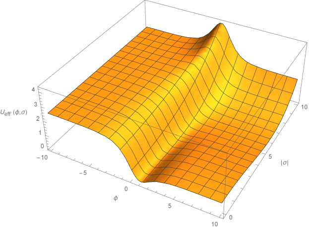
  Figure 1: Qualitative shape of the two-dimensional plot for the effective scalar potential $U_{eff}$.

  becomes a dynamically induced $SU(2)\times U(1)$ spontaneous symmetry breaking Higgs-like potential with a Higgs “vacuum” at $|\sigma_{\rm vac}|=\frac{1}{m_{0}}\sqrt{f_{1}}$.

• Relations (24)-(25) allow the following natural identification of the scales of the parameters: $\Lambda_{0}\sim 10^{-122}M^{4}_{Pl}$ (current epoch observable cosmological constant); $f_{1}\sim f_{2}\sim M^{4}_{EW}$ and $m_{0}\sim M_{EW}$ ($M_{EW}$ being the electroweak mass scale); $M_{1}\sim M_{2}\sim 10^{-8}M_{Pl}^{4}$ corresponding to the “early” universe’s energy scale of inflation being of order $10^{-2}M_{Pl}$.

Concerning confrontation with the observational data, the viability of the present model (in a slightly simplified form without the Higgs scalar, which as already mentioned does not influence the slow-roll inflationary dynamics) has been analyzed and confirmed numerically in Ref.Guendelman:2014bva . The results for the tensor-to-scalar ratio $r\simeq 10^{-3}$ and for the scalar spectral index $n_{s}\simeq 0.96$ which are in a good agreement with the latest Further detailed numerical studies on the NRVF models have been presented in Refs. Staicova:2016pfd ; Staicova:2018bdy ; Staicova:2019ksr .

Let us also note that Ref.Guendelman:2014bva (for an earlier version, see Guendelman:2002js ) exhibits an explicit realization of the cosmological “seesaw” mechnaism through the NRVF formulation, as well as it yields an additional “emergent universe” cosmological solution without a “Big-Bang” initial singularity. For a brief illustration of the latter effects let us consider the “inflaton-only” NRVF action studied in Guendelman:2014bva (for simplicity we skip the $R^{2}$ term):

$$S=\int d^{4}x\,\Phi_{1}(A)\Bigl{[}R+X_{\varphi}-f_{1}e^{-\alpha\varphi}\Bigr{]}+\int d^{4}x\,\Phi_{2}(B)\Bigl{[}-b\,e^{-\alpha\varphi}\,X_{\varphi}+f_{2}e^{-2\alpha\varphi}-\frac{\Phi_{0}(C)}{\sqrt{-g}}\Bigr{]}\;,$$ (26)

where $b$ is an additional dimensionless parameter.

The “inflaton” potential in the Einstein frame (analog of (23)) is:

$$U_{\rm eff}(\varphi)=\frac{1}{4\chi_{2}}\bigl{(}f_{1}e^{-\alpha\varphi}+M_{1}\bigr{)}^{2}\bigl{(}f_{2}e^{-2\alpha\varphi}+M_{2}\bigr{)}^{-1}$$ (27)

so that on the (-) and (+) “inflaton” flat regions $U_{\rm eff}(\varphi)$ reduces to: $U_{(-)}\simeq\frac{f_{1}^{2}}{4\chi_{2}\,f_{2}}$ and $U_{(+)}\simeq\frac{M_{1}^{2}}{4\chi_{2}\,M_{2}}$, accordingly. Therefore, choosing $f_{1}\sim f_{2}\sim 10^{-8}M^{4}_{Pl}$ conforming to the inflationary scale, and taking $M_{1}\sim M^{4}_{EW}$ and $M_{2}\sim M^{4}_{Pl}$ we achieve $U_{(+)}\sim 10^{-122}M^{4}_{Pl}$ vastly smaller than $U_{(-)}$. If we take $\alpha\to-\alpha$ in (26) the roles of $f_{1,2}$ and $M_{1,2}$ are interchanged.

Similar “seesaw” effect is found in Refs.Benisty:2019vej ; Benisty:2020xqm where the scalar potential is extracted from the slow-roll parameters. . Furthermore, the NRVF model (26) yields in EInstein-frame “emergent universe” solution for the range of the $b$-parameter: $-4(2-\sqrt{3})<b\frac{f_{1}}{f_{2}}<-1$.

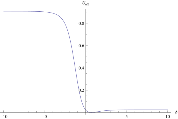
Figure 2: Qualitative shape of the one-dimensional plot for the effective scalar potential $U_{eff}$.

4 Dynamical Generation of Inflation in Metric Formulation

Let us now consider a substantionally truncated version of the model (17) without any matter fields, involving few non-Riemannian volume elements Benisty:2019tno :

$$S=\int d^{4}x\Bigl{\{}\Phi_{1}(A)\Bigl{[}R(g)-2\Lambda_{0}\frac{\Phi_{1}(A)}{\sqrt{-g}}\Bigr{]}+\Phi_{2}(B)\frac{\Phi_{0}(C)}{\sqrt{-g}}\Bigr{\}}\;,$$ (28)

where now unlike (17) $R(g)\equiv g^{\mu\nu}R_{\mu\nu}\bigl{(}\Gamma(g)\bigr{)}$ is the scalar curvature in the second order (metric) formalism ($\Gamma^{\lambda}_{\mu\nu}(g)$ being the Levi-Civita connection w.r.t. $g_{\mu\nu}$).

The equations of motion w.r.t. auxiliary tensor gauge fields $A_{\mu\nu\lambda}$, $\Phi_{2}(B)$ and $\Phi_{1}(C)$ are special cases of the dynamical constraint Eqs.(18)-(19) with all matter field terms being zero, which again introduce the three free integration constants $M_{1,2},\,\chi_{2}$.

Passage to the physical Einstein frame is again realized via the conformal transformation (21), however this time we have to use the well-known formulas for conformal transformations within the metric formalism (Dabrowski:2008kx ; bars indicate magnitudes in the ${\bar{g}}_{\mu\nu}$-frame):

$$R_{\mu\nu}(g)=R_{\mu\nu}(\bar{g})-3\frac{{\bar{g}}_{\mu\nu}}{\chi_{1}}{\bar{g}}^{\kappa\lambda}\partial_{\kappa}\chi_{1}^{1/2}\partial_{\lambda}\chi_{1}^{1/2}+\chi_{1}^{-1/2}\bigl{(}{\bar{\nabla}}_{\mu}{\bar{\nabla}}_{\nu}\chi_{1}^{1/2}+{\bar{g}}_{\mu\nu}{\bar{\Box}}\chi_{1}^{1/2}\bigr{)}\;,$$ (29)

with $\chi_{1}\equiv\frac{\Phi_{1}(A)}{\sqrt{-g}}$. Redefining $\chi_{1}$ as $\chi_{1}=\exp{\bigl{(}u/\sqrt{3}\bigr{)}}$ allows to write the Einstein-frame NRVF action in the form:

$$S_{\rm EF}=\int d^{4}x\sqrt{-{\bar{g}}}\Bigl{[}R({\bar{g}})-\frac{1}{2}{\bar{g}}^{\mu\nu}\partial_{\mu}u\partial_{\nu}u-U_{\rm eff}(u)\Bigr{]}\;,$$ (30)

$$U_{\rm eff}(u)=2\Lambda_{0}-M_{1}\exp{\bigl{(}-\frac{u}{\sqrt{3}}\bigr{)}}+\chi_{2}M_{2}\exp{\bigl{(}-2\frac{u}{\sqrt{3}}\bigr{)}}\;.$$ (31)

Thus, from the original pure-gravity NRVF action (28) we derived a physical Einstein-frame action (30)-(31) containing a dynamically created scalar field $u$ with a non-trivial effective scalar potential $U_{\rm eff}(u)$ (31) entirely dynamically generated by the initial non-Riemannian volume elements in (28) because of the appearance of the free integration constants $M_{1,2},\,\chi_{2}$ in their respective equations of motion. There are two main features of the effective potential (31) which are relevant for cosmological applications with the dynamically created field $u$ as an “inflaton”.

• $U_{\rm eff}(u)$ (31) possesses one flat region for large positive values of $u$ where $U_{\rm eff}(u)\simeq 2\Lambda_{0}$, which corresponds to “early” universe’ inflationary evolution with energy scale $2\Lambda_{0}$.

• $U_{\rm eff}(u)$ (31) has a stable minimum for a small finite value $u=u_{*}$ where $e^{-u_{*}/\sqrt{3}}=M_{1}/(2\chi_{2}M_{2})$.

• The region around the stable minimum at $u=u_{*}$ correspond to “late” universe’ evolution where the minimum value of the potential:

  $$U_{\rm eff}(u_{*})=2\Lambda_{0}-\frac{M_{1}^{2}}{4\chi_{2}M_{2}}\equiv 2\Lambda_{\rm DE}$$ (32)

  is the dark energy density value.

Remark. The effective potential $U_{\rm eff}$ (31) generalizes the well-known Starobinsky inflationary potential Starobinsky:1979ty ((23) reduces to Starobinsky potential upon taking the following special values for the parameters: $\Lambda_{0}=\frac{1}{4}M_{1}=\frac{1}{2}\chi_{2}M_{2}$).

In Ref.Benisty:2019tno a thorough analysis has been performed of the slow-roll inflationary dynamics driven by the dynamically created “inflaton” $u$ with its dynamically generated effective potential (31), including explicit calculation of the standard slow-roll parameters $\epsilon$ and $\eta$, as well we have obtained explicit expressions for the tensor-to-scalar ratio $r$ and the scalar spectral index $n_{s}$ of density perturbations as functions of the number of e-folds ${\mathcal{N}}=\log a$ ($a$ being the Friedmann scale factor):

$$r\simeq\frac{12}{\Bigl{[}{\mathcal{N}}+\frac{\sqrt{3}}{4}u_{i}({\mathcal{N}})+c_{0}\Bigr{]}^{2}},\quad n_{s}\simeq 1-\frac{r}{4}-\sqrt{\frac{r}{3}},$$ (33)

with $c_{0}\equiv\frac{\sqrt{3}}{2}-\frac{3}{4}\log\Bigl{(}2\bigl{(}1+2/\sqrt{3}\bigr{)}\Bigr{)}$. $u_{i}({\mathcal{N}})$ is the value of the “unflaton” at the start of inflation as function of ${\mathcal{N}}$.

For a plausible assumption about the scales of $M_{1,2},\,\chi_{2}$ and taking ${\mathcal{N}}=60$ $e$-folds till end of inflation the observables are predicted to be: $n_{s}\approx 0.969\;\;,\;\;r\approx 0.0026$, which conform to the PLANCK constraints Akrami:2018odb ($0.95<n_{s}<0.97\;\;,\;\;r<0.064$).

5 Dynamical Spacetime Formulation

Let us now observe that the non-Riemannian volume element $\Omega=\Phi(B)$ (3) on a Riemannian manifold can be rewritten using Hodge duality (here $D=4$) in terms of a vector field $\chi^{\mu}=\frac{1}{3!}\frac{1}{\sqrt{-g}}\varepsilon^{\mu\nu\kappa\lambda}B_{\nu\kappa\lambda}$ so that $\Omega$ becomes $\Omega(\chi)=\partial_{\mu}\bigl{(}\sqrt{-g}\chi^{\mu}\bigr{)}$,  i.e. it is a non-canonical volume element different from $\sqrt{-g}$, but still involving the metric. It can be represented alternatively through a Lagrangian multiplier action term yielding covariant conservation of a specific energy-momentum tensor of the form ${\mathcal{T}}^{\mu\nu}=g^{\mu\nu}{\mathcal{L}}$:

$$\mathcal{S}_{(\chi)}=\int d^{4}x\sqrt{-g}\,\chi_{\mu;\nu}{\mathcal{T}}^{\mu\nu}=\int d^{4}x\partial_{\mu}\bigl{(}\sqrt{-g}\chi^{\mu}\bigr{)}\bigl{(}-{\mathcal{L}}\bigr{)}\;,$$ (34)

where $\chi_{\mu;\nu}=\partial_{\nu}\chi_{\mu}-\Gamma_{\mu\nu}^{\lambda}\chi_{\lambda}$. The vector field $\chi_{\mu}$ is called “dynamical space time vector”, because of the energy density of ${\mathcal{T}}^{00}$ is a canonically conjugated momentum w.r.t. $\chi_{0}$, which is what we expected from a dynamical time.

In what follows we will briefly consider a new class of gravity-matter theories based on the ordinary Riemannian volume element $\sqrt{-g}$ but involving action terms of the form (34) where now ${\mathcal{T}}^{\mu\nu}$ is of more general form than ${\mathcal{T}}^{\mu\nu}=g^{\mu\nu}{\mathcal{L}}$. This new formalism is called “dynamical spacetime formalism” Guendelman:2009ck ; Benisty:2016ybt due to the above remark on $\chi_{0}$.

Ref.Benisty:2018qed describes a unification between dark energy and dark matter by introducing a quintessential scalar field in addition to the dynamical time action. The total Lagrangian reads:

$$\mathcal{L}=\frac{1}{2}R+\chi_{\mu;\nu}{\mathcal{T}}^{\mu\nu}-\frac{1}{2}g^{\alpha\beta}\phi_{,\alpha}\phi_{,\beta}-V(\phi),$$ (35)

with energy-momentum tensor ${\mathcal{T}}^{\mu\nu}=-\frac{1}{2}\phi^{,\mu}\phi^{,\nu}$. From the variation of the Lagrangian term $\chi_{\mu;\nu}{\mathcal{T}}^{\mu\nu}$ with respect to the vector field $\chi_{\mu}$, the covariant conservation of the energy-momentum tensor $\nabla_{\mu}{\mathcal{T}}^{\mu\nu}=0$ is implemented. The latter within the FLRW framework forces the kinetic term of the scalar field to behave as a dark matter component:

$$\nabla_{\mu}{\mathcal{T}}^{\mu\nu}=0\quad\Rightarrow\quad\dot{\phi}^{2}=\frac{2\Omega_{m0}}{a^{3}}.$$ (36)

where $\Omega_{m0}$ is an integration constant. The variation with respect to the scalar field $\phi$ yields a current:

$$-V^{\prime}(\phi)=\nabla_{\mu}j^{\mu},\quad j^{\mu}=\frac{1}{2}\phi_{,\nu}(\chi^{\mu;\nu}+\chi^{\nu;\mu})+\phi^{,\mu}$$ (37)

For constant potential $V(\phi)=\Omega_{\Lambda}=const$ the current is covariantly conserved. In the FLRW setting, where the dynamical time ansatz introduces only a time component $\chi_{\mu}=(\chi_{0},0,0,0)$, the variation (37) gives:

$$\dot{\chi}_{0}-1=\xi\,a^{-3/2},$$ (38)

where $\xi$ is an integration constant. Accordingly, the FLRW energy density and pressure read:

$$\rho=\left(\dot{\chi}_{0}-\frac{1}{2}\right)\dot{\phi}^{2}+V,\quad p=\frac{1}{2}\dot{\phi}^{2}(\dot{\chi}_{0}-1)-V.$$ (39)

Plugging the relations (36,38) into the density and the pressure terms (39) yields the following simple form of the latter:

$$\rho=\Omega_{\Lambda}+\frac{\xi\Omega_{m0}}{a^{9/2}}+\frac{\Omega_{m0}}{a^{3}},\quad p=-\Omega_{\Lambda}+\frac{\xi\Omega_{m0}}{2\,a^{9/2}}.$$ (40)

In (40) there are 3 components for the "dark fluid": dark energy with $\omega_{\Lambda}=-1$, dark matter with $\omega_{m}=0$ and an additional equation of state $\omega_{\xi}=1/2$. For non-vanishing and negative $\xi$ the additional part introduces a minimal scale parameter, which avoids singularities. If the dynamical time is equivalent to the cosmic time $\chi_{0}=t$, we obtain $\xi=0$ from Eq.(38), whereupon the density and the pressure terms (40) coincide with those from the $\Lambda$CDM model precisely. The additional part (for $\xi\neq 0$) fits to the late time accelerated expansion data Anagnostopoulos:2019myt .

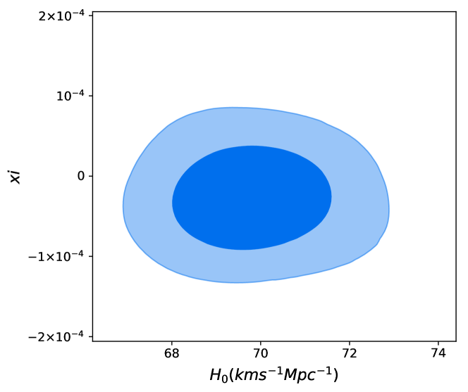
Figure 3: The posterior distribution for the simplest case of DST cosmology in the parameter space $\xi$ vs. $H_{0}$.

In order to constraint our model, we deploy the following data sets: Cosmic Chronometers (CC) exploit the evolution of differential ages of passive galaxies at different redshifts to directly constrain the Hubble parameter Jimenez:2001gg . We use uncorrelated 30 CC measurements of $H(z)$ discussed in Moresco:2012by ; Moresco:2012jh ; Moresco:2015cya ; Moresco:2016mzx . As Standard Candles (SC) we use uncorrelated measurements of the Pantheon Type Ia supernova Scolnic:2017caz that were collected in Anagnostopoulos:2020ctz . In addition, we use the uncorrelated data points from different Baryon Acoustic Oscillations (BAO) collected in Benisty:2020otr from Percival:2009xn ; Beutler:2011hx ; Busca:2012bu ; Anderson:2012sa ; Seo:2012xy ; Ross:2014qpa ; Tojeiro:2014eea ; Bautista:2017wwp ; deCarvalho:2017xye ; Ata:2017dya ; Abbott:2017wcz ; Molavi:2019mlh . Studies of the BAO features in the transverse direction provide a measurement of $D_{H}(z)/r_{d}=c/H(z)r_{d}$, with the comoving angular diameter distance defined in Hogg:2020ktc ; Martinelli:2020hud . In our database we use the parameters $D_{A}=D_{M}/(1+z)$ and

$$D_{V}(z)\equiv[zD_{H}(z)D_{M}^{2}(z)]^{1/3}.$$ (41)

which is a combination of the BAO peak coordinates. $r_{d}$ is the sound horizon at the drag epoch. Finally, for very precise "line-of-sight" (or "radial") observations, BAO can also measure directly the Hubble parameter Benitez:2008fs .

The posterior distribution yields: $\Omega_{m}=0.2811\pm 0.0743$, $\Omega_{\Lambda}=0.7187\pm 0.07351$, $\xi=(-2.776\pm 3.023)\cdot 10^{5}$ and with the Hubble parameter $H_{0}=69.72\pm 1.239Mpc/(km/sec)$. Benisty:2018gzx shows that with higher dimensions, the solution derived from the Lagrangian (35) describes inflation, where the total volume oscillates and the original scale parameter exponentially grows.

The dynamical spacetime Lagrangian can be generalized to yield a diffusive energy-momentum tensor. Ref. Calogero:2013zba shows that the diffusion equation has the form:

$$\nabla_{\mu}{\mathcal{T}}^{\mu\nu}=3\sigma j^{\nu},\quad j^{\mu}_{;\mu}=0,$$ (42)

where $\sigma$ is the diffusion coefficient and $j^{\mu}$ is a current source. The covariant conservation of the current source indicates the conservation of the number of the particles. By introducing the vector field $\chi_{\mu}$ in a different part of the Lagrangian:

$$\mathcal{L}_{(\chi,A)}=\chi_{\mu;\nu}{\mathcal{T}}^{\mu\nu}+\frac{\sigma}{2}(\chi_{\mu}+\partial_{\mu}A)^{2},$$ (43)

the energy-momentum tensor ${\mathcal{T}}^{\mu\nu}$ gets a diffusive source. From a variation with respect to the dynamical space time vector field $\chi_{\mu}$ we obtain:

$$\nabla_{\nu}{\mathcal{T}}^{\mu\nu}=\sigma(\chi^{\mu}+\partial^{\mu}A)=f^{\mu},$$ (44)

a current source $f^{\mu}=\sigma(\chi^{\mu}+\partial^{\mu}A)$ for the energy-momentum tensor. From the variation with respect to the new scalar $A$, a covariant conservation of the current emerges $f^{\mu}_{;\mu}=0$. The latter relations correspond to the diffusion equation (42). Refs.Benisty:2017eqh ; Benisty:2017rbw ; Benisty:2017lmt ; Bahamonde:2018uao study the cosmological solution using the energy-momentum tensor ${\mathcal{T}}^{\mu\nu}=-\frac{1}{2}g^{\mu\nu}\phi^{,\lambda}\phi_{\lambda}$. The total Lagrangian reads:

$$\mathcal{L}=\frac{1}{2}R-\frac{1}{2}g^{\alpha\beta}\phi_{,\alpha}\phi_{,\beta}-V(\phi)\\ +\chi_{\mu;\nu}{\mathcal{T}}^{\mu\nu}+\frac{\sigma}{2}(\chi_{\mu}+\partial_{\mu}A)^{2}.$$ (45)

The FLRW solution unifies the dark energy and the dark matter originating from one scalar field with possible diffusion interaction. Ref.Benisty:2018oyy investigates more general energy-momentum tensor combinations and shows that asymptotically all of the combinations yield $\Lambda$CDM model as a stable fixed point. Banerjee:2019kgu shows that the DST theories and Diffusive extensions can describe a Lagrangian formulation for Running Vacuum Models.

6 Scale Invariance, Fifth Force in Fermionic and Dust Matter

In this class of theories the fifth force problem can be solved, this can be checked most simply in a theory with two volume elements (integration measure densities) Guendelman:1999qt ; Guendelman:1999tb , where at least one of them was a non-canonical one and short-termed “two-measure theory” (TMT). The result is expected to be generic however. This model has a number of remarkable properties if fermions are included in a self-consistent way Guendelman:1999tb . In this case, the constraint that arises in the TMT models in the Palatini formalism can be represented as an equation for $\chi\equiv\Phi/\sqrt{-g}$, in which the left side has an order of the vacuum energy density, and the right side (in the case of non-relativistic fermions) is proportional to the fermion density. Moreover, it turns out that even cold fermions have a (non-canonical) pressure $P_{f}^{noncan}$ and the corresponding contribution to the energy-momentum tensor has the structure of a cosmological constant term which is proportional to the fermion density. The remarkable fact is that the right hand side of the constraint coincide with $P_{f}^{noncan}$. This allows us to construct a cosmological model Guendelman:2012vc of the late universe in which dark energy is generated by a gas of non-relativistic neutrinos without the need to introduce into the model a specially designed scalar field.

In models with a scalar field, the requirement of scale invariance of the initial actionGuendelman:1999qt plays a very constructive role. It allows to construct a modelGuendelman:2006af where without fine tuning we have realized: absence of initial singularity of the curvature; k-essence; inflation with graceful exit to zero cosmological constant. Of particular interest are scale invariant models in which both fermions and a dilaton scalar field $\phi$ are present. Then it turns out that the Yukawa coupling of fermions to $\phi$ is proportional to $P_{f}^{noncan}$. As a result, it follows from the constraint, that in all cases when fermions are in states which constitute a regular barionic matter, the Yukawa coupling of fermions to dilaton has an order of ratio of the vacuum energy density to the fermion energy density Guendelman:2006ji . Thus, the theory provides a solution of the 5-th force problem without any fine tuning or a special design of the model. Besides, in the described states, the regular Enstein’s equations are reproduced. In the opposite case, when fermions are very deluted, e.g. in the model of the late Universe filled with a cold neutrino gas, the neutrino dark energy appears in such a way that the dilaton $\phi$ dynamics is closely correlated with that of the neutrino gas Guendelman:2006ji .

Scale invariant model containing a dilaton $\phi$ and dust (as a model of matter)Guendelman:2007ph possesses similar features. Dilaton to matter coupling "constant" $f$ appears to be dependent of the matter density. To see this more explicitly, let us consider the action containing a non Riemannian measure $\Phi$ which is a total divergence and is invariant under the global scale transformations:

$$g_{\mu\nu}\rightarrow e^{\theta}g_{\mu\nu},\quad\Gamma^{\mu}_{\alpha\beta}\rightarrow\Gamma^{\mu}_{\alpha\beta},\quad\phi\rightarrow\phi-\frac{M_{p}}{\alpha}\theta,\quad\Phi\rightarrow e^{2\theta}\Phi$$ (46)

where $\theta=const$. It is convenient to represent the action in the following form:

$$S = S_{g}+S_{\phi}+S_{m}$$ (47)

$$S_{g} = -\frac{1}{\kappa}\int(\Phi+b_{g}\sqrt{-g})R(\Gamma,g)e^{\alpha\phi/M_{p}}d^{4}x\,;$$

$$S_{\phi} = \int e^{\alpha\phi/M_{p}}\left[(\Phi+b_{\phi}\sqrt{-g})\frac{1}{2}g^{\mu\nu}\phi_{,\mu}\phi_{,\nu}-\left(\Phi V_{1}+\sqrt{-g}V_{2}\right)e^{\alpha\phi/M_{p}}\right]d^{4}x\,;$$

$$S_{m} = \int(\Phi+b_{m}\sqrt{-g})L_{m}d^{4}x\,,$$

where the Lagrangian for the matter, as collection of particles, which provides the scale invariance of $S_{m}$ reads

$$L_{m}=-m\sum_{i}\int e^{\frac{1}{2}\alpha\phi/M_{p}}\sqrt{g_{\alpha\beta}\frac{dx_{i}^{\alpha}}{d\lambda}\frac{dx_{i}^{\beta}}{d\lambda}}\,\frac{\delta^{4}(x-x_{i}(\lambda))}{\sqrt{-g}}d\lambda$$ (48)

where $\lambda$ is an arbitrary parameter. For simplicity we consider the collection of the particles with the same mass parameter $m$. We assume in addition that $x_{i}(\lambda)$ do not participate in the scale transformations (46). We will assume that $d\vec{x}_{i}/d\lambda\equiv 0$ for all particles. It is convenient to proceed in the frame where $g_{0l}=0$,   $l=1,2,3$. Then the particle density is defined by

$$n(\vec{x})=\sum_{i}\frac{1}{\sqrt{-g_{(3)}}}\delta^{(3)}(\vec{x}-\vec{x}_{i}(\lambda))$$ (49)

where $g_{(3)}=\det(g_{kl})$ and

$$S_{m}=-m\int d^{4}x(\Phi+b_{m}\sqrt{-g})\,n(\vec{x})\,e^{\frac{1}{2}\alpha\phi/M_{p}}$$ (50)

It turns out that when working with the new metric ($\phi$ remains the same)

$$\tilde{g}_{\mu\nu}=e^{\alpha\phi/M_{p}}(\zeta+b_{g})g_{\mu\nu},$$ (51)

which we call the Einstein frame, the connection becomes Riemannian. Notice that $\tilde{g}_{\mu\nu}$ is invariant under the scale transformations (46). The transformation (51) causes the transformation of the particle density

$$\tilde{n}(\vec{x})=(\zeta+b_{g})^{-3/2}\,e^{-\frac{3}{2}\alpha\phi/M_{p}}\,n(\vec{x})$$ (52)

After the change of variables to the Einstein frame (51) and some simple algebra, the gravitational equations take the standard GR form

$$G_{\mu\nu}(\tilde{g}_{\alpha\beta})=\frac{\kappa}{2}T_{\mu\nu}^{eff}$$ (53)

where $G_{\mu\nu}(\tilde{g}_{\alpha\beta})$ is the Einstein tensor in the Riemannian space-time with the metric $\tilde{g}_{\mu\nu}$. The components of the effective energy-momentum tensor are as follows:

$$T_{00}^{eff} = \frac{\zeta+b_{\phi}}{\zeta+b_{g}}\left(\dot{\phi}^{2}-\tilde{g}_{00}X\right)$$

$$+ \tilde{g}_{00}\left[V_{eff}(\phi;\zeta,M)-\frac{\delta\cdot b_{g}}{\zeta+b_{g}}X+\frac{3\zeta+b_{m}+2b_{g}}{2\sqrt{\zeta+b_{g}}}\,m\,\tilde{n}\right]$$

$$T_{ij}^{eff} = \frac{\zeta+b_{\phi}}{\zeta+b_{g}}\left(\phi_{,k}\phi_{,l}-\tilde{g}_{kl}X\right)$$

$$+ \tilde{g}_{kl}\left[V_{eff}(\phi;\zeta,M)-\frac{\delta\cdot b_{g}}{\zeta+b_{g}}X+\frac{\zeta-b_{m}+2b_{g}}{2\sqrt{\zeta+b_{g}}}\,m\,\tilde{n}\right]$$

Here the following notations have been used:

$$X\equiv\frac{1}{2}\tilde{g}^{\alpha\beta}\phi_{,\alpha}\phi_{,\beta}\qquad and\qquad\delta=\frac{b_{g}-b_{\phi}}{b_{g}}$$ (56)

and the function $V_{eff}(\phi;\zeta)$ is defined by

$$V_{eff}(\phi;\zeta)=\frac{b_{g}\left[M^{4}e^{-2\alpha\phi/M_{p}}+V_{1}\right]-V_{2}}{(\zeta+b_{g})^{2}}$$ (57)

The dilaton $\phi$ field equation in the Einstein frame is as follows

$$\frac{1}{\sqrt{-\tilde{g}}}\partial_{\mu}\left[\frac{\zeta+b_{\phi}}{\zeta+b_{g}}\sqrt{-\tilde{g}}\tilde{g}^{\mu\nu}\partial_{\nu}\phi\right]-\frac{\alpha}{M_{p}}\,\frac{(\zeta+b_{g})M^{4}e^{-2\alpha\phi/M_{p}}-(\zeta-b_{g})V_{1}-2V_{2}-\delta b_{g}(\zeta+b_{g})X}{(\zeta+b_{g})^{2}}$$

$$=\frac{\alpha}{M_{p}}\,\frac{\zeta-b_{m}+2b_{g}}{2\sqrt{\zeta+b_{g}}}\,m\,\tilde{n}$$ (58)

In the above equations, the scalar field $\zeta$ is determined as a function $\zeta(\phi,X,\tilde{n})$ by means of the following constraint:

$$\frac{(b_{g}-\zeta)\left(M^{4}e^{-2\alpha\phi/M_{p}}+V_{1}\right)-2V_{2}}{(\zeta+b_{g})^{2}}-\frac{\delta\cdot b_{g}X}{\zeta+b_{g}}=\frac{\zeta-b_{m}+2b_{g}}{2\sqrt{\zeta+b_{g}}}\,m\,\tilde{n}$$

(59)

One should now pay attention to the interesting result that the explicit $\tilde{n}$ dependence involving the same form of $\zeta$ dependence

$$\frac{\zeta-b_{m}+2b_{g}}{2\sqrt{\zeta+b_{g}}}\,m\,\tilde{n}$$ (60)

appears simultaneously in the dust contribution to the pressure (through the last term in Eq. (6)), in the effective dilaton to dust coupling (in the r.h.s. of Eq. (58)) and in the r.h.s. of the constraint (59).

Let us analyze consequences of this wonderful coincidence in the case when the matter energy density (modeled by dust) is much larger than the dilaton contribution to the dark energy density in the space region occupied by this matter. Evidently this is the condition under which all tests of Einstein’s GR, including the question of the fifth force, are fulfilled. if the dust is in the normal conditions there is a possibility to provide the desirable feature of the dust in GR: it must be pressureless. This is realized provided that in normal conditions (n.c.) the following equality holds with extremely high accuracy:

$$\zeta^{(n.c.)}\approx b_{m}-2b_{g}$$ (61)

Remind that we have assumed $b_{m}>b_{g}$. Then $\zeta^{(n.c.)}+b_{g}>0$, and the transformation (51) and the subsequent equations in the Einstein frame are well defined. Inserting (61) in the last term of Eq. (6) we obtain the effective dust energy density in normal conditions

$$\rho_{m}^{(n.c.)}=2\sqrt{b_{m}-b_{g}}\,m\tilde{n}$$ (62)

When we get only a slight deviation of from $\zeta$ from $b_{m}-2b_{g}$, when the matter energy density is many orders of magnitude larger than the dilaton contribution to the dark energy density, we obtain an effective 5th force coupling $f$. For this look at the $\phi$-equation in the form (58) and estimate the Yukawa type coupling constant in the r.h.s. of this equation. In fact, using the constraint (59) and representing the particle density in the form $\tilde{n}\approx N/\upsilon$ where $N$ is the number of particles in a volume $\upsilon$, one can make the following estimation for the effective dilaton to matter coupling "constant" $f$ defined by the Yukawa type interaction term $f\tilde{n}\phi$ (if we were to invent an effective action whose variation with respect to $\phi$ would result in Eq. (58)):

$$f\equiv\alpha\frac{m}{M_{p}}\,\frac{\zeta-b_{m}+2b_{g}}{2\sqrt{\zeta+b_{g}}}\approx\alpha\frac{m}{M_{p}}\,\frac{\zeta-b_{m}+2b_{g}}{2\sqrt{b_{m}-b_{g}}}\sim\frac{\alpha}{M_{p}}\,\frac{\rho_{vac}}{\tilde{n}}\approx\alpha\frac{\rho_{vac}\upsilon}{NM_{p}}$$ (63)

becomes less than the ratio of the "mass of the vacuum" in the volume occupied by the matter to the Planck mass. The model yields this kind of "Archimedes law" without any especial (intended for this) choice of the underlying action and without fine tuning of the parameters. The model not only explains why all attempts to discover a scalar force correction to Newtonian gravity were unsuccessful so far but also predicts that in the near future there is no chance to detect such corrections in the astronomical measurements as well as in the specially designed fifth force experiments on intermediate, short (like millimeter) and even ultrashort (a few nanometer) ranges. This prediction is alternative to predictions of other known models.

Finally, we want to point out fundamental differences of our solution of the fifth force force problem to the Chameleon approach. The important point to make is that we are talking of totally different mechanisms, in the Chameleon model, the proposed quintessential scalar, the Chameleon field has a mass in vacuum which is very small, of the order of the Hubble parameter for example (or in any case very very small). The Chameleon scalar however becomes massive in presence of dense matter, in compact objects, like Earth, a typical number for this mass has been cited, $m^{-1}\sim 60_{mm}$ Khoury:2003aq . This is why a quanta of this scalar field can penetrate only into a thin shell of the body in the depth about 60micrometer, and the fifth force acts only on the thin shell. This is a way the Chameleon model is argued to explain the smallness of the fifth force. In our case there is no mass generation whatsoever since for our dilaton field, what happens here is the vanishing of the effective coupling constant between the dilaton field and the dense matter, while the dilaton keeps is mass zero or very close to zero. The elimination of interaction between our dilaton field and dense matter is total and absolute, in comparison, a Chameleon wave can suffer a total reflection from a dense matter region, in such a situation it will not be a total elimination of the fifth force, but it may be hard indeed to prepare such an experiment. The elimination of the fifth force in the Chameleon model is argued to exist because in a spherically symmetric static configuration of a macroscopic object only a very small shell of the object can be a source of the Chameleon scalar, while in our case there would be no source for the scalar, not even the edge or surface of the dense object or at any place of the dense object. Higher-order theories of gravity also have been also studied in connection of fifth force suppression and have been shown to produce an explicit realization of the Chameleon scenario from first principles Capozziello:2007eu ; Capozziello:2012ie .

References

- [1] E. I. Guendelman. Scale invariance, new inflation and decaying lambda terms. Mod. Phys. Lett., A14:1043–1052, 1999.
- [2] E. I. Guendelman and A. B. Kaganovich. Dynamical measure and field theory models free of the cosmological constant problem. Phys. Rev., D60:065004, 1999.
- [3] Eduardo Guendelman, Emil Nissimov, Svetlana Pacheva, and Mahary Vasihoun. A New Mechanism of Dynamical Spontaneous Breaking of Supersymmetry. Bulg. J. Phys., 41(2):123–129, 2014.
- [4] Eduardo Guendelman, Emil Nissimov, and Svetlana Pacheva. Vacuum structure and gravitational bags produced by metric-independent space–time volume-form dynamics. Int. J. Mod. Phys. A, 30(22):1550133, 2015.
- [5] Frank Gronwald, Uwe Muench, Alfredo Macias, and Friedrich W. Hehl. Volume elements of space-time and a quartet of scalar fields. Phys. Rev., D58:084021, 1998.
- [6] M. Spivak, editor. Calculus On Manifolds – a Modern Approach To Classical Theorem Of Advanced Calculus. CRC Press, 2018.
- [7] Eduardo Guendelman, Emil Nissimov, and Svetlana Pacheva. Gravity-Assisted Emergent Higgs Mechanism in the Post-Inflationary Epoch. Int. J. Mod. Phys. D, 25(12):1644008, 2016.
- [8] M. Henneaux and C. Teitelboim, editors. Quantization of Gauge Systems. Princeton Univ. Press,, 1991.
- [9] H. Rothe and K. Rothe, editors. Classical and Quantum Dynamics of Constrained Hamiltonian Systems. World Scientific,, 2010.
- [10] M. Henneaux and C. Teitelboim. The Cosmological Constant and General Covariance. Phys. Lett., B222:195–199, 1989.
- [11] Eduardo Guendelman, Ramón Herrera, Pedro Labrana, Emil Nissimov, and Svetlana Pacheva. Emergent Cosmology, Inflation and Dark Energy. Gen. Rel. Grav., 47(2):10, 2015.
- [12] Eduardo Guendelman, Emil Nissimov, and Svetlana Pacheva. Unified Dark Energy and Dust Dark Matter Dual to Quadratic Purely Kinetic K-Essence. Eur. Phys. J., C76(2):90, 2016.
- [13] D. Benisty, E. I. Guendelman, E. Nissimov, and S. Pacheva. CDM as a Noether Symmetry in Cosmology. 2020.
- [14] Denitsa Staicova and Michail Stoilov. Cosmological aspects of a unified dark energy and dust dark matter model. Mod. Phys. Lett., A32(01):1750006, 2016.
- [15] J.D. Bekenstein. Gravitation and Spontaneous Symmetry Breaking. Found. Phys., 16:409–422, 1986.
- [16] Lars Brink, Viatcheslav Mukhanov, Eliezer Rabinovici, and K.K. Phua, editors. Jacob Bekenstein: The Conservative Revolutionary. WSP, 2020.
- [17] David Benisty, Eduardo Guendelman, Emil Nissimov, and Svetlana Pacheva. Quintessential Inflation with Dynamical Higgs Generation as an Affine Gravity. Symmetry, 12:734, 2020.
- [18] Denitsa Staicova and Michail Stoilov. Cosmological Solutions from a Multi-Measure Model with Inflaton Field. Symmetry, 11(11):1387, 2019.
- [19] Denitsa Staicova and Michail Stoilov. Cosmology from multimeasure multifield model. Int. J. Mod. Phys., A34(19):1950099, 2019.
- [20] E. I. Guendelman and O. Katz. Inflation and transition to a slowly accelerating phase from SSB of scale invariance. Class. Quant. Grav., 20:1715–1728, 2003.
- [21] David Benisty, Eduardo I. Guendelman, and Emmanuel N. Saridakis. The Scale Factor Potential Approach to Inflation. 2019.
- [22] David Benisty and Eduardo I. Guendelman. Lorentzian Quintessential Inflation. Int. J. Mod. Phys., D10:1142, 2020.
- [23] David Benisty, Eduardo Guendelman, Emil Nissimov, and Svetlana Pacheva. Dynamically Generated Inflation from Non-Riemannian Volume Forms. 2019.
- [24] Mariusz P. Dabrowski, Janusz Garecki, and David B. Blaschke. Conformal transformations and conformal invariance in gravitation. Annalen Phys., 18:13–32, 2009.
- [25] Alexei A. Starobinsky. Spectrum of relict gravitational radiation and the early state of the universe. JETP Lett., 30:682–685, 1979. [,767(1979)].
- [26] Y. Akrami et al. Planck 2018 results. X. Constraints on inflation. Astron. Astrophys., 641:A10, 2020.
- [27] E. I. Guendelman. Gravitational Theory with a Dynamical Time. Int. J. Mod. Phys., A25:4081–4099, 2010.
- [28] David Benisty and E. I. Guendelman. Radiation Like Scalar Field and Gauge Fields in Cosmology for a theory with Dynamical Time. Mod. Phys. Lett., A31(33):1650188, 2016.
- [29] David Benisty and Eduardo I. Guendelman. Unified dark energy and dark matter from dynamical spacetime. Phys. Rev., D98(2):023506, 2018.
- [30] Fotios K. Anagnostopoulos, David Benisty, Spyros Basilakos, and Eduardo I. Guendelman. Dark energy and dark matter unification from dynamical space time: observational constraints and cosmological implications. JCAP, 1906(06):003, 2019.
- [31] Raul Jimenez and Abraham Loeb. Constraining cosmological parameters based on relative galaxy ages. Astrophys. J., 573:37–42, 2002.
- [32] Michele Moresco, Licia Verde, Lucia Pozzetti, Raul Jimenez, and Andrea Cimatti. New constraints on cosmological parameters and neutrino properties using the expansion rate of the Universe to z 1.75. JCAP, 1207:053, 2012.
- [33] M. Moresco et al. Improved constraints on the expansion rate of the Universe up to z 1.1 from the spectroscopic evolution of cosmic chronometers. JCAP, 1208:006, 2012.
- [34] Michele Moresco. Raising the bar: new constraints on the Hubble parameter with cosmic chronometers at z 2. Mon. Not. Roy. Astron. Soc., 450(1):L16–L20, 2015.
- [35] Michele Moresco, Lucia Pozzetti, Andrea Cimatti, Raul Jimenez, Claudia Maraston, Licia Verde, Daniel Thomas, Annalisa Citro, Rita Tojeiro, and David Wilkinson. A 6% measurement of the Hubble parameter at : direct evidence of the epoch of cosmic re-acceleration. JCAP, 1605:014, 2016.
- [36] D.M. Scolnic et al. The Complete Light-curve Sample of Spectroscopically Confirmed SNe Ia from Pan-STARRS1 and Cosmological Constraints from the Combined Pantheon Sample. Astrophys. J., 859(2):101, 2018.
- [37] Fotios K. Anagnostopoulos, Spyros Basilakos, and Emmanuel N. Saridakis. Observational constraints on Barrow holographic dark energy. Eur. Phys. J., C80(9):826, 2020.
- [38] David Benisty and Denitsa Staicova. Testing Low-Redshift Cosmic Acceleration with the Complete Baryon Acoustic Oscillations data collection. 2020.
- [39] Will J. Percival et al. Baryon Acoustic Oscillations in the Sloan Digital Sky Survey Data Release 7 Galaxy Sample. Mon. Not. Roy. Astron. Soc., 401:2148–2168, 2010.
- [40] Florian Beutler, Chris Blake, Matthew Colless, D. Heath Jones, Lister Staveley-Smith, Lachlan Campbell, Quentin Parker, Will Saunders, and Fred Watson. The 6dF Galaxy Survey: Baryon Acoustic Oscillations and the Local Hubble Constant. Mon. Not. Roy. Astron. Soc., 416:3017–3032, 2011.
- [41] Nicolas G. Busca et al. Baryon Acoustic Oscillations in the Ly- forest of BOSS quasars. Astron. Astrophys., 552:A96, 2013.
- [42] Lauren Anderson et al. The clustering of galaxies in the SDSS-III Baryon Oscillation Spectroscopic Survey: Baryon Acoustic Oscillations in the Data Release 9 Spectroscopic Galaxy Sample. Mon. Not. Roy. Astron. Soc., 427(4):3435–3467, 2013.
- [43] Hee-Jong Seo et al. Acoustic scale from the angular power spectra of SDSS-III DR8 photometric luminous galaxies. Astrophys. J., 761:13, 2012.
- [44] Ashley J. Ross, Lado Samushia, Cullan Howlett, Will J. Percival, Angela Burden, and Marc Manera. The clustering of the SDSS DR7 main Galaxy sample – I. A 4 per cent distance measure at . Mon. Not. Roy. Astron. Soc., 449(1):835–847, 2015.
- [45] Rita Tojeiro et al. The clustering of galaxies in the SDSS-III Baryon Oscillation Spectroscopic Survey: galaxy clustering measurements in the low redshift sample of Data Release 11. Mon. Not. Roy. Astron. Soc., 440(3):2222–2237, 2014.
- [46] Julian E. Bautista et al. The SDSS-IV extended Baryon Oscillation Spectroscopic Survey: Baryon Acoustic Oscillations at redshift of 0.72 with the DR14 Luminous Red Galaxy Sample. Astrophys. J., 863:110, 2018.
- [47] E. de Carvalho, A. Bernui, G. C. Carvalho, C. P. Novaes, and H. S. Xavier. Angular Baryon Acoustic Oscillation measure at from the SDSS quasar survey. JCAP, 1804:064, 2018.
- [48] Metin Ata et al. The clustering of the SDSS-IV extended Baryon Oscillation Spectroscopic Survey DR14 quasar sample: first measurement of baryon acoustic oscillations between redshift 0.8 and 2.2. Mon. Not. Roy. Astron. Soc., 473(4):4773–4794, 2018.
- [49] T. M. C. Abbott et al. Dark Energy Survey Year 1 Results: Measurement of the Baryon Acoustic Oscillation scale in the distribution of galaxies to redshift 1. Mon. Not. Roy. Astron. Soc., 483(4):4866–4883, 2019.
- [50] Z. Molavi and A. Khodam-Mohammadi. Observational tests of Gauss-Bonnet like dark energy model. Eur. Phys. J. Plus, 134(6):254, 2019.
- [51] Natalie B. Hogg, Matteo Martinelli, and Savvas Nesseris. Constraints on the distance duality relation with standard sirens. 2020.
- [52] M. Martinelli et al. Euclid: Forecast constraints on the cosmic distance duality relation with complementary external probes. 2020.
- [53] N. Benitez et al. Measuring Baryon Acoustic Oscillations along the line of sight with photometric redshifs: the PAU survey. Astrophys. J., 691:241–260, 2009.
- [54] David Benisty and Eduardo I. Guendelman. Inflation compactification from dynamical spacetime. Phys. Rev., D98(4):043522, 2018.
- [55] Simone Calogero and Hermano Velten. Cosmology with matter diffusion. JCAP, 1311:025, 2013.
- [56] David Benisty and E. I. Guendelman. Interacting Diffusive Unified Dark Energy and Dark Matter from Scalar Fields. Eur. Phys. J., C77(6):396, 2017.
- [57] David Benisty and E. I. Guendelman. Unified DE–DM with diffusive interactions scenario from scalar fields. Int. J. Mod. Phys., D26(12):1743021, 2017.
- [58] David Benisty and Eduardo I. Guendelman. A transition between bouncing hyper-inflation to CDM from diffusive scalar fields. Int. J. Mod. Phys., A33(20):1850119, 2018.
- [59] Sebastian Bahamonde, David Benisty, and Eduardo I. Guendelman. Linear potentials in galaxy halos by Asymmetric Wormholes. Universe, 4(11):112, 2018.
- [60] David Benisty, Eduardo Guendelman, and Zbigniew Haba. Unification of dark energy and dark matter from diffusive cosmology. Phys. Rev., D99(12):123521, 2019.
- [61] S. Banerjee, D. Benisty, and E. I. Guendelman. Running Vacuum from Dynamical Spacetime Cosmology. 2019.
- [62] E. I. Guendelman and A. B. Kaganovich. Neutrino generated dynamical dark energy with no dark energy field. Phys. Rev., D87(4):044021, 2013.
- [63] E.I. Guendelman and A.B. Kaganovich. Fine Tuning Free Paradigm of Two Measures Theory: K-Essence, Absence of Initial Singularity of the Curvature and Inflation with Graceful Exit to Zero Cosmological Constant State. Phys. Rev. D, 75:083505, 2007.
- [64] E. I. Guendelman and A. B. Kaganovich. Exotic low density fermion states in the two measures field theory: Neutrino dark energy. Int. J. Mod. Phys., A21:4373–4406, 2006.
- [65] E.I. Guendelman and A.B. Kaganovich. Absence of the Fifth Force Problem in a Model with Spontaneously Broken Dilatation Symmetry. Annals Phys., 323:866–882, 2008.
- [66] Justin Khoury and Amanda Weltman. Chameleon fields: Awaiting surprises for tests of gravity in space. Phys. Rev. Lett., 93:171104, 2004.
- [67] Salvatore Capozziello and Shinji Tsujikawa. Solar system and equivalence principle constraints on f(R) gravity by chameleon approach. Phys. Rev. D, 77:107501, 2008.
- [68] Salvatore Capozziello and Mariafelicia De Laurentis. The dark matter problem from f(R) gravity viewpoint. Annalen Phys., 524:545–578, 2012.