EMPRESS. II.
Highly Fe-Enriched Metal-poor Galaxies with $\sim 1.0$ (Fe/O)_⊙ and $0.02$ (O/H)_⊙ :
Possible Traces of Super Massive ($>300M_{\odot}$) Stars in Early Galaxies

Abstract

We present element abundance ratios and ionizing radiation of local young low-mass ($\sim 10^{6}M_{\odot}$) extremely metal poor galaxies (EMPGs) with a 2% solar oxygen abundance (O/H)_⊙ and a high specific star-formation rate (sSFR$\sim$300 Gyr^-1), and other (extremely) metal poor galaxies, which are compiled from Extremely Metal-Poor Representatives Explored by the Subaru Survey (EMPRESS) and the literature. Weak emission lines such as [Fe iii]4658 and He ii4686 are detected in very deep optical spectra of the EMPGs taken with 8m-class telescopes including Keck and Subaru (Kojima et al., 2020; Izotov et al., 2018), enabling us to derive element abundance ratios with photoionization models. We find that neon- and argon-to-oxygen ratios are comparable to those of known local dwarf galaxies, and that the nitrogen-to-oxygen abundance ratios (N/O) are lower than 20% (N/O)_⊙ consistent with the low oxygen abundance. However, the iron-to-oxygen abundance ratios (Fe/O) of the EMPGs are generally high; the EMPGs with the 2%-solar oxygen abundance show high Fe/O ratios of $\sim 90-140$% (Fe/O)_⊙, which are unlikely explained by suggested scenarios of Type Ia supernova iron productions, iron’s dust depletion, and metal-poor gas inflow onto previously metal-riched galaxies with solar abundances. Moreover, the EMPGs with the 2%-solar oxygen abundance have very high He ii4686/H$\beta$ ratios of $\sim$1/40, which are not reproduced by existing models of high-mass X-ray binaries with progenitor stellar masses $<$ $120M_{\odot}$. Comparing stellar-nucleosynthesis and photoionization models with a comprehensive sample of EMPGs identified by this and previous EMPG studies, we propose that both the high Fe/O ratios and the high He ii4686/H$\beta$ ratios are explained by the past existence of super massive ($>300M_{\odot}$) stars, which may evolve into intermediate-mass black holes ($\gtrsim 100M_{\odot}$).

1. INTRODUCTION

The early universe is dominated by a large number of young, low-mass, metal-poor galaxies. Theoretical arguments suggest that the first galaxies are formed at $z\sim 10$–$20$ from gas already metal-enriched by Pop-III (i.e., metal free) stars. According to hydrodynamical simulations (e.g., Wise et al., 2012), the first galaxies are created in dark matter (DM) mini halos with $\sim 10^{8}M_{\odot}$ and have low stellar masses ($\log$($M_{\star}$/$M_{\odot}$)$\sim$4–6), low metallicities ($Z\sim 0.1$–$1\%Z_{\odot}$), and high specific star-formation rates (${\rm sSFR}\sim 100$ Gyr^-1) at $z\sim 10$. The typical stellar mass is remarkably small, comparable to those of star clusters. Such cluster-like galaxies are undergoing early phases of the galaxy formation. One of critical goals of the modern cosmology is to understand the early-phase galaxy formation by probing the cluster-like, star-forming galaxies (SFGs).

The stellar population and the star-formation history are critical information to understand galaxies undergoing the early-phase star formation. Element abundances such as iron (Fe) and nitrogen (N) are good tracers of the past star formation and the stellar population because these elements are produced and ejected by the different stellar populations at different ages. First, iron elements are effectively produced and released into ISM by type-Ia supernovae (SNe) $\sim$1 Gyr after the start of the star formation. The type-Ia SNe are triggered by gas accretion from a main sequence star onto a white dwarf, whose progenitor weighs $\sim$1–10 $M_{\odot}$ (e.g., Nomoto et al., 2013), in a binary system. The type-Ia SNe start contributing to the increase of iron-to-oxygen ratio (Fe/O) at the age of $\sim$1 Gyr (e.g., Steidel et al., 2016). As reported in studies of Galactic stars (Bensby & Feltzing, 2006; Lecureur et al., 2007; Bensby et al., 2013), the increasing Fe/O trend is seen in a metallicity range of $Z_{*}/Z_{\odot}\gtrsim 0.2$ (corresponding to $12$+$\log({\rm O/H})$$\gtrsim$8.0). Below $12$+$\log({\rm O/H})$$\sim$8.0 (or $\lesssim$1 Gyr), the core-collapse SNe mainly contribute to the production and release of iron and oxygen. Under the assumption of this mechanism, low-mass, metal-poor, young SFGs are expected to have a low Fe/O ratio due to their young ages. Second, nitrogen elements trace activities of massive stars and low- and intermediate-mass stars at low and high metallicities, respectively. As suggested by previous studies (Pérez-Montero & Contini, 2009; Pérez-Montero et al., 2013; Andrews & Martini, 2013), nitrogen-to-oxygen ratios (N/O) of SFGs present a plateau in the range of $12$+$\log({\rm O/H})$$\lesssim$8.0 and a positive slope at higher metallicities as a function of metallicity. Model calculations of the N/O evolution (e.g., Vincenzo et al., 2016) also support this trend. The plateau basically results from the primary nucleosynthesis of massive stars, while the positive slope is mainly attributed to the secondary nucleosynthesis of low- and intermediate-mass stars (e.g., Vincenzo et al., 2016). In the nitrogen-enrichment mechanism, low-mass, metal-poor, young SFGs may have a low N/O ratio because of their low metallicities and young ages.

Ionizing radiation is another key to understand the stellar population of galaxies in the early-phase star formation. Ionizing radiation is produced by massive stars and/or a hot accretion disk around compact objects such as black holes (BHs). Observational studies (López-Sánchez & Esteban, 2010; Shirazi & Brinchmann, 2012; Senchyna et al., 2017; Schaerer et al., 2019) have suggested that SFGs show strong He ii4686 emission lines represented by He ii4686/H$\beta$$\sim$1/300–1/30. Especially, the He ii4686/H$\beta$ shows an increasing trend as metallicity decreases in the range of $12$+$\log({\rm O/H})$$<$8.0. The He ii4686 line is sensitive to ionizing photons above 54.4 eV, which are not abundant in radiation of O- and B-type hot stars. Under the assumption of stellar radiation, Xiao et al. (2018) have created nebular emission models with the combination of the photoionization code cloudy (Ferland et al., 2013) and the bpass (Binary Population and Spectral Synthesis) code (Stanway et al., 2016; Eldridge et al., 2017). The Xiao et al. (2018) models predict He ii4686/H$\beta$$\lesssim$1/1000, well below the observed He ii4686/H$\beta$ ratios of $\sim$1/300 to $\sim$1/30 (Schaerer et al., 2019). This means that the main contributors of He ii4686 are not hot stars. Schaerer et al. (2019) have estimated He ii4686/H$\beta$ ratios with high mass X-ray binary (HMXB) models of Fragos et al. (2013a, b), and suggested that high He ii4686/H$\beta$ ratios can be partly explained by the HMXB models. However, the HMXB models still do not explain the high He ii4686/H$\beta$ ratios for galaxies with a high H$\beta$ equivalent width, $\textrm{EW}_{0}$(H$\beta$)$>$100 Å (i.e., younger than 5 Myr). Schaerer et al. (2019) suggest another possible contribution from old stellar population and/or shock-heated gas. Saxena et al. (2020b) investigate a connection between the He ii4686 and X-ray emission of 18 He ii-emitting galaxies at $z\sim 2$–4, concluding that the observed He ii4686/H$\beta$ ratios and X-ray intensities are not explained by the HMXBs simultaneously. The mass range of the sample is $\log$($M_{\star}$/$M_{\odot}$)$=$8.8–10.7 (Saxena et al., 2020a, b), which corresponds to $\sim$0.2–1.0 $Z_{\odot}$ under the assumption of the mass-metallicity relation at $z\sim 2$–4 (Shapley et al., 2017). The conclusion of Saxena et al. (2020b) may only be applicable to relatively mature galaxies with intermediate masses and metallicities, in contrast to metal-poor galaxies at $z\sim 0$ (e.g., Schaerer et al., 2019). Senchyna et al. (2020) also investigate the connection between the He ii4686 and X-ray emission with a sample of 11 local galaxies. Senchyna et al. (2020) conclude that HMXBs are not dominant sources of the He⁺-ionizing photons, although a possibility of soft X-ray sources such as intermediate-mass black holes (IMBHs) is not ruled out. In the sample of Senchyna et al. (2020), 4 galaxies show low metallicities (0.06–0.1$Z_{\odot}$) and low H$\beta$ equivalent widths ($\textrm{EW}_{0}$(H$\beta$)$\sim$50–100Å), and 3 galaxies show high metallicities ($>$0.1$Z_{\odot}$) and high H$\beta$ equivalent widths ($\textrm{EW}_{0}$(H$\beta$)$\sim$200–400Å). Galaxies with very low metallicities ($\sim$0.01$Z_{\odot}$) and high H$\beta$ equivalent widths ($\textrm{EW}_{0}$(H$\beta$)$\gtrsim$100Å) at the same time are missing in the sample of Senchyna et al. (2020). In summary, the main contributor of the He ii4686 emission is still under debate, especially at low metallicities and high H$\beta$ equivalent widths, which are expected to be metal-poor galaxies undergoing very early phases of the galaxy evolution.

In the local universe, extremely metal-poor galaxies (EMPGs) have been discovered (e.g., Izotov & Thuan, 1998; Thuan et al., 2005; Izotov et al., 2009, 2018, 2019; Ly et al., 2014) by exploiting wide-field data such as Sloan Digital Sky Survey (SDSS, York et al., 2000). These galaxies have low metallicities, $12$+$\log({\rm O/H})$$\sim$7.0–7.2, low stellar masses, $\log$($M_{\star}$/$M_{\odot}$)$\sim$6–8, and high sSFR, $\sim 100$ Gyr^-1. Such local EMPGs are regarded as local analogs of high-$z$ galaxies because they have low metallicities, low stellar masses, and large emission line equivalent widths similar to low-mass galaxies with $\log$($M_{\star}$/$M_{\odot}$)$\sim$6–8 at $z\sim 2$–$3$ (Christensen et al., 2012a, b; Stark et al., 2014; Vanzella et al., 2017) and $z\sim 6$–$7$ (Stark et al., 2015; Mainali et al., 2017). However, the stellar mass ranges of the previous studies, $\log$($M_{\star}$/$M_{\odot}$)$\sim$6–8, are not as low as cluster-like galaxies in the early-phase of the galaxy formation, $\log$($M_{\star}$/$M_{\odot}$)$\sim$4–6, as described above. To reach a lower mass range than the previous EMPG studies (e.g., SDSS, $i$-band limiting magnitude $\sim$21 mag), deeper, wide-field imaging survey has been expected.

We have initiated a new EMPG survey with wide-field optical imaging data obtained in Subaru/Hyper Suprime-Cam (HSC; Miyazaki et al., 2012, 2018; Komiyama et al., 2018; Kawanomoto et al., 2018; Furusawa et al., 2018) Subaru Strategic Program (HSC-SSP; Aihara et al., 2018) in Kojima et al. (2020, Paper I hereafter). The new EMPG survey has been named “Extremely Metal-Poor Representatives Explored by the Subaru Survey” (EMPRESS). We have created a source sample based on the deep, wide-field HSC-SSP data, which covers $\sim 500$ deg² area with a $5\sigma$ limit of $\sim 26$ mag in Paper I. In this EMPRESS project, we try to select low-mass EMPGs with a large $\textrm{EW}_{0}$(H$\alpha$) (e.g., $\gtrsim$800 Å) because our motivation is to discover local counterparts of high-$z$, low-mass galaxies whose specific star-formation rate (sSFR) is expected to be high ($\gtrsim$10 Gyr^-1, e.g., Ono et al., 2010; Stark et al., 2017; Elmegreen & Elmegreen, 2017; Harikane et al., 2018), which are expected to be undergoing very early phases of the galaxy evolution.

This paper is the second paper from our EMPRESS project. The detailed sample selection and results of the first spectroscopic observations have been reported in Paper I. These paper will be followed by other papers in which we investigate details of size and morphology, and kinematics of our EMPG sample (e.g., Isobe et al., 2020, Paper III hereafter). The outline of this paper is as follows. In Section 2, we briefly explain our samples selected from the Subaru HSC-SSP data and the SDSS data. In Section 3, we describe our optical spectroscopy carried out for our EMPG candidates and explain the reduction and calibration processes of our spectroscopy data. In Section 4, we measure emission line fluxes and estimate galaxy properties such as stellar mass, star-formation rate, metallicity, and element abundance. Section 5 shows results and discussions of element abundance ratios and ionizing radiation. Then Section 6 summarizes this paper. Throughout this paper, magnitudes are on the AB system (Oke & Gunn, 1983). We adopt the following cosmological parameters, $(h,\Omega_{m},\Omega_{\Lambda})=(0.7,0.3,0.7)$. The definition of the solar metallicity is given by $12$+$\log({\rm O/H})$=8.69 (Asplund et al., 2009). We also define an EMPG as a galaxy with $12$+$\log({\rm O/H})$$<$7.69 (i.e., $Z/Z_{\odot}$$<$0.1) in this paper, which is almost the same as in previous metal-poor galaxy studies (e.g., Kunth & Östlin, 2000; Izotov et al., 2012; Guseva et al., 2017).

2. SAMPLE

This paper uses samples obtained by Paper I. In Paper I, we select the EMPG candidates from HSC-SSP and SDSS data with our machine learning (ML) classifier. We briefly describe selections of EMPG candidates in this section. Hereafter, these candidates chosen from the HSC-SSP and SDSS source catalogs are called “HSC-EMPG candidates” and “SDSS-EMPG candidates”, respectively.

2.1. HSC-EMPG candidates

We use the HSC-SSP internal data of the S17A and S18A data releases, which are explained in the second data release (DR2) paper of HSC-SSP (Aihara et al., 2019). Although the HSC-SSP survey data are taken in three layers of Wide, Deep, and UltraDeep, we only use the Wide field layer in this study. In the HSC-SSP S17A and S18A data releases, images were reduced with the HSC pipeline, hscPipe v5.4 and v6.7 (Bosch et al., 2018), respectively, with codes of the Large Synoptic Survey Telescope (LSST) software pipeline (Ivezić et al., 2019a; Axelrod et al., 2010; Jurić et al., 2015; Ivezić et al., 2019b). The pipeline conducts the bias subtraction, flat fielding, image stacking, astrometry and zero-point magnitude calibration, source detection, and magnitude measurement. As reported in Paper I, there are slight differences in our results between S17A and S18A data due to the different pipeline versions. Thus, although part of the S17A and S18A data are duplicated, we use both S17A and S18A data in this study to maximize the size of our EMPG sample. The details of the observations, data reduction, detection, photometric catalog, and pipeline are described in Aihara et al. (2019) and Bosch et al. (2018). We use cmodel magnitudes (Bosch et al., 2018) corrected for Milky-Way dust extinction (Schlegel et al., 1998) in the estimation of the total magnitudes of a source.

Below we explain how we construct an HSC source catalog, from which we select EMPG candidates. We use isolated or cleanly deblended sources that fall within $griz$-band images. We also require that none of the pixels in their footprints are interpolated, none of the central 3 $\times$ 3 pixels are saturated, none of the central 3 $\times$ 3 pixels suffer from cosmic rays, and there are no bad pixels in their footprints. Then we exclude sources whose cmodel magnitude or centroid position measurements have a problem. We require a detection in the $griz$-band images. We mask sources close to a bright star (Coupon et al., 2018; Aihara et al., 2019) in the S18A data. Here we select objects whose photometric measurements are brighter than 5$\sigma$ limiting magnitudes, $g<26.5$, $r<26.0$, $i<25.8$, and $z<25.2$ mag, which are estimated by Ono et al. (2018) with 1.5-arcsec diameter circular apertures. We also require that the photometric measurement errors are less than 0.1 mag in $griz$ bands. Finally, we obtain 17,912,612 and 40,407,765 sources in total from the HSC-SSP S17A and S18A data, respectively, with the selection criteria explained above. The effective area is 205.82 and 508.84 deg² in the HSC-SSP S17A and S18A data, respectively. See Paper I for details of our HSC source sample.

We select EMPG candidates from the HSC-SSP source catalog in four steps: i) An initial rough selection based on colors, extendedness, and blending. ii) the ML classifier selection. iii) Transient object removal by measuring the flux variance in multi-epoch images. iv) Visual inspection of the $gri$-composite images. Refer to Paper I for the selection details. Eventually, we obtain 12 and 21 HSC-EMPG candidates from the S17A and S18A catalogs, respectively. We find that 6 out of the HSC-EMPG candidates are duplicated between the S17A and S18A catalogs. Thus the number of our independent HSC-EMPG candidates is 27 ($=$12$+$21$-$6). A magnitude range of the 27 HSC-EMPG candidates is $i=19.3$–$24.3$ mag.

2.2. SDSS-EMPG candidates

We construct a SDSS source catalog from the 13th release (DR13; Albareti et al., 2017) of the SDSS photometry data. Although the SDSS data are $\sim$5 mag shallower ($i_{\rm lim}$$\sim$21 mag) than HSC-SSP data ($i_{\rm lim}$$\sim$26 mag), we also select EMPG candidates from the SDSS data to complement brighter EMPGs. Here we select objects whose photometric measurements are brighter than SDSS limiting magnitudes, $u<22.0$, $g<22.2$, $r<22.2$, $i<21.3$, and $z<21.3$ mag. We only obtain objects whose magnitude measurement errors are $<$0.1 mag in $ugriz$ bands. Note that we use Modelmag for the SDSS data. Among flags in the PhotoObjALL catalog, we require that a clean flag is “1” (i.e., True) to remove objects with photometry measurement issues. The clean flag eliminates the duplication, deblending/interpolation problems, suspicious detections, and detections at the edge of an image. We also remove objects with a True cosmic-ray flag and/or a True blended flag, which often mimics a broad-band excess in photometry. We reject relatively large objects with a ninety-percent petrosian radius greater than 10 arcsec to eliminate contamination by HII regions in nearby spiral galaxies. Finally, we derive 31,658,307 sources in total from the SDSS DR13 photometry data. The total unique area of SDSS DR13 data is 14,555 deg².

We select EMPG candidates from the SDSS source catalog similarly to the HSC source catalog in Section 2.1. After the selection, we derive 86 SDSS-EMPG candidates from the SDSS source catalog, whose $i$-band magnitudes range $i=14.8$–$20.9$ mag. One out of the 86 candidates (HSC J1429$-$0110) is also selected as an HSC-EMPG candidate in Section 2.1. Details are described in Paper I.

3. SPECTROSCOPIC DATA

In this section, we explain our spectroscopic data of 10 galaxies described in Paper I, which are selected from our HSC and SDSS source catalogs and confirmed to be metal-poor galaxies. We have identified that the 2 out of the 10 metal-poor galaxies (HSC J1631$+$4426 and SDSS J2115$-$1734) satisfy the EMPG condition of $Z<0.10Z_{\odot}$ with metallicity estimates based on the electron temperature measurement. HSC J1631$+$4426 shows a metallicity of 0.016 $Z_{\odot}$, which is the lowest metallicity reported to date. In addition to the 10 metal-poor galaxies, we include another EMPG from the literature (J0811$+$4730, Izotov et al., 2018) in the sample of this paper. J0811$+$4730 has the second lowest metallicity of 0.019 $Z_{\odot}$ reported to date.

In paper I, we report on our spectroscopy of the 10 metal-poor galaxies performed with 4 spectrographs of the Low Dispersion Survey Spectrograph 3 (LDSS-3) and the Magellan Echellette Spectrograph (MagE) on Magellan telescope, the Deep Imaging Multi-Object Spectrograph (DEIMOS) on Keck-II telescope, and the Faint Object Camera And Spectrograph (FOCAS) on Subaru telescope. Although the spectroscopy and reduction are detailed in Paper I, we briefly summarize them in Sections 3.1–3.4. In Section 3.5, we newly report very faint emission lines detected in our spectroscopy, such as [O iii]4363, [Ar iv]4711, [Fe iii]4658, He ii4686, [N ii]6584, and [Ar iii]7136, which are required to estimate element abundance ratios and constrain the FUV spectral hardness (Section 1). Signal to noise ratios of our spectra depend on observational conditions (e.g., telescope, instrument, and integration time) and object brightnesses. Thus, the detection of such faint emission lines also depends on the observational conditions and object brightnesses.

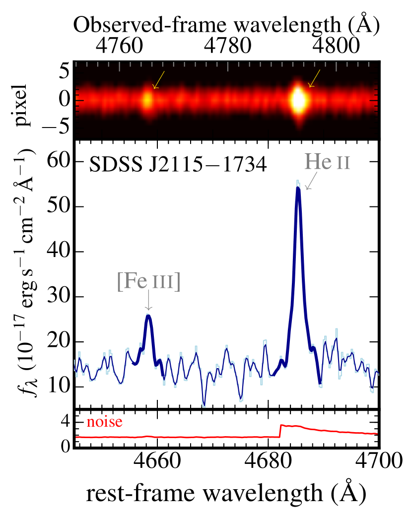
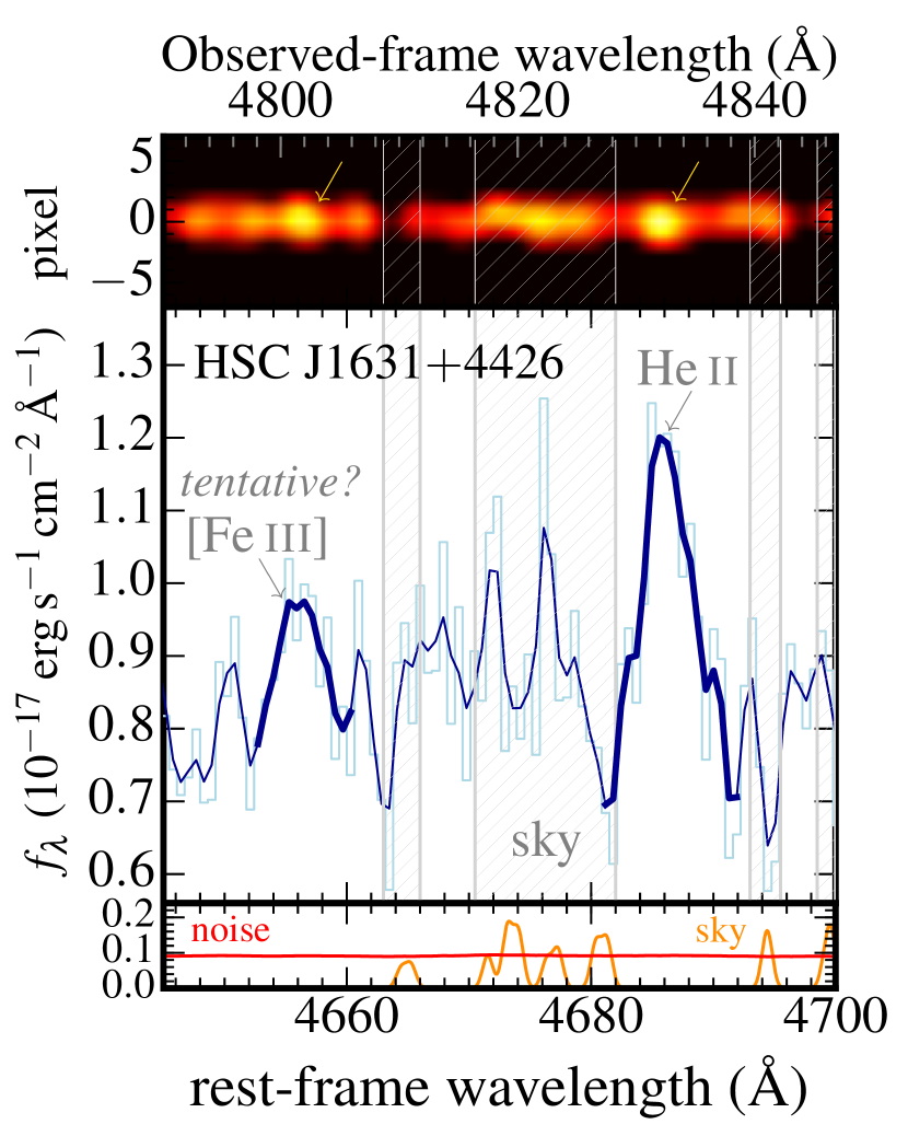
Figure 1.— Spectra of SDSS J2115$-$1734 (left) and HSC J1631$+$4426 (right) taken in our MagE and FOCAS spectroscopy, respectively, around the [Fe iii]4658 and He ii4686 emission lines. The top, center, and bottom panels show 2D spectra, signal spectra, and noise$+$sky spectra, respectively. In the center panel, the light blue line is the un-smoothed background subtracted spectrum, while the dark blue line is spectra smoothed with a Gaussian profile. The shaded regions indicate positions of the sky emission lines. In the bottom panel, we exhibit a noise spectrum with the red lines. The orange line show a sky emission spectrum (in arbitrary units) modeled with the sky emission data of Hanuschik (2003). For SDSS J2115$-$1734, no sky emission line falls on the wavelength range of this panel.

3.1. Magellan/LDSS-3

We conducted spectroscopy for one galaxy selected from our HSC catalog (HSC J1429$-$0110) with LDSS-3 at Magellan telescope. We used the VPH-ALL grism with the $0.\!\!^{\prime\prime}75$$\times$4^′ long-slit, which was placed at the offset position two-arcmin away from the center of the long-slit mask so that the spectroscopy could cover the bluer side. The exposure time was 3,600 seconds. The spectroscopy covered $\lambda\sim$3,700–9,500 Å with a spectral resolution of $R\equiv\lambda/\Delta\lambda\sim$ 860.

We used the iraf package to reduce and calibrate the LDSS-3 data. The reduction and calibration processes include the bias subtraction, flat fielding, one-dimensional (1D) spectrum subtraction, sky subtraction, wavelength calibration, flux calibration, and atmospheric-absorption correction. A one-dimensional spectrum was derived from an aperture centered on the blue compact component of our galaxies. A standard star, CD-32  9972 was used in the flux calibration. The wavelengths were calibrated with the HeNeAr lamp. Atmospheric absorption was corrected with the extinction curve at Cerro Tololo Inter-American Observatory (CTIO). Our LDSS-3 spectroscopy may have been affected by the atmospheric refraction because a slit was not necessarily placed perpendicular to the horizon (i.e., at a parallactic angle) in our spectroscopy, which may lead to the wavelength-dependent slit loss. The slit angles of each target are determined so that we can simultaneously observe multiple emission regions. To estimate the wavelength-dependent slit loss $SL(\lambda)$ carefully, we made a model of the atmospheric refraction.

3.2. Magellan/MagE

We carried out spectroscopy for 8 galaxies selected from our HSC and SDSS catalogs (HSC J2314$+$0154, HSC J1142$-$0038, SDSS J0002$+$1715, SDSS J1642$+$2233, SDSS J2115$-$1734, SDSS J2253$+$1116, SDSS J2310$-$0211, and SDSS J2253$+$1116) with MagE of Magellan telescope. We used the echellette grating with the $0.\!\!^{\prime\prime}85$$\times$10^′′ or $1.\!\!^{\prime\prime}2$$\times$10^′′ longslits. The exposure time was 1,800 or 3,600 seconds, depending on luminosities of the galaxies. The MagE spectroscopy covered $\lambda\sim$3,100–10,000 Å with a spectral resolution of $R\equiv\lambda/\Delta\lambda\sim$ 4,000.

To reduce the raw data taken with MagE, we used the MagE pipeline from Carnegie Observatories Software Repository. The MagE pipeline has been developed on the basis of the Carpy package (Kelson et al., 2000; Kelson, 2003). The bias subtraction, flat fielding, scattered light subtraction, two-dimensional (2D) spectrum subtraction, sky subtraction, wavelength calibration, cosmic-ray removal, 1D-spectrum subtraction were conducted with the MagE pipeline. Details of these pipeline processes are described on the web site of Carnegie Observatories Software Repository mentioned above. One-dimensional spectra were subtracted by summing pixels along the slit-length direction on a 2D spectrum.

We conducted the flux calibration with the standard star, Feige 110, using iraf routines. Wavelengths were calibrated with emission lines of the ThAr lamp. Spectra of each order were calibrated separately and combined with the weight of electron counts to generate a single 1D spectrum. Atmospheric absorption was corrected in the same way as in Section 3.1. Our MagE spectroscopy may have been also affected by the atmospheric refraction for the same reason as the LDSS-3 spectroscopy. Thus, we corrected the wavelength-dependent slit loss carefully in the same manner as the LDSS-3 spectroscopy described in Section 3.1.

3.3. Keck/DEIMOS

We conducted spectroscopy for one galaxy selected from our HSC catalog (HSC J1631$+$4426) with DEIMOS of the Keck-II telescope. We used the multi-object mode with the $0.\!\!^{\prime\prime}8$ slit width. The exposure time was 2,400 seconds. We used the 600ZD grating and the BAL12 filter with a blaze wavelength at 5,500 Å. The DEIMOS spectroscopy covered $\lambda\sim$3,800–8,000 Å with a spectral resolution of $R\equiv\lambda/\Delta\lambda\sim$1,500.

We used the iraf package to reduce and calibrate the DEIMOS data. The reduction and calibration processes were the same as the LDSS-3 data explained in Section 3.1. A standard star, G191B2B was used in the flux calibration. Wavelengths were calibrated with the NeArKrXe lamp. Atmospheric absorption was corrected under the assumption of the extinction curve at Mauna Kea Observatories. We only used a spectrum within the wavelength range of $\lambda>$4,900 Å, which was free from the stray light (see Paper I for its detail). We ignore the effect of the atmospheric refraction here because we only use a red side ($\lambda>$4,900 Å) of DEIMOS data, which is insensitive to the atmospheric refraction. We also confirm that the effect of the atmospheric refraction is negligible with the models described in Section 3.1. In the DEIMOS data, we only used line flux ratios normalized to an H$\beta$ flux. Emission line fluxes were scaled with an H$\beta$ flux by matching an H$\beta$ flux obtained with DEIMOS to one obtained with FOCAS (see Section 3.4).

3.4. Subaru/FOCAS

We carried out deep spectroscopy for one galaxy selected from our HSC catalog (HSC J1631$+$4426) with FOCAS installed on the Subaru telescope (PI: T. Kojima). This object was the same object as in the Keck/DEIMOS Spectroscopy (Section 3.3) and observed again with FOCAS with a longer integration time of 10,800 sec. We used the long slit mode with the $2.\!\!^{\prime\prime}0$ slit width. The exposure time was 10,800 seconds ($=$3 hours). We used the 300R grism and the L550 filter with a blaze wavelength at 7,500 Å in a 2nd order. The FOCAS spectroscopy covered $\lambda\sim$3,400–5,250 Å with a spectral resolution of $R$$\equiv$$\lambda/\Delta\lambda$$=$400 with the $2.\!\!^{\prime\prime}0$ slit width.

We used the iraf package to reduce and calibrate the FOCAS data. The reduction and calibration processes were the same as the LDSS-3 data explained in Section 3.1. A standard star, BD$+$28 4211 was used in the flux calibration. Wavelengths were calibrated with the ThAr lamp. Atmospheric absorption was corrected in the same way as in Section 3.3. Our FOCAS spectroscopy covered $\lambda\sim$3,800–5,250 Å, which was complementary to the DEIMOS spectroscopy described in Section 3.3, whose spectrum was reliable only in the range of $\lambda>$4900 Å. We ignore the atmospheric refraction here because FOCAS is equipped with the atmospheric dispersion corrector. Because an H$\beta$ line was over-wrapped in FOCAS and DEIMOS spectroscopy, we used an H$\beta$ line flux to scale the emission line fluxes obtained in the DEIMOS observation (see Section 3.3).

3.5. Weak Emission Lines in the Spectra

In our spectroscopy, we have detected many emission lines including very faint emission lines such as [O iii]4363, [Ar iv]4711, [Fe iii]4658, He ii4686, [N ii]6584, and [Ar iii]7136. These faint emission lines are required to estimate element abundance ratios and constrain the FUV spectral hardness. Especially, the [Fe iii]4658 and He ii4686 lines are key in this paper, which enable us to investigate the Fe/O abundance ratios and the very hard EUV radiation, as described in Section 1.

In Figure 1, we show two spectra of SDSS J2115$-$1734 and HSC J1631$+$4426 (classified as EMPGs in Paper I) around the [Fe iii]4658 and He ii4686 emission lines. In the left panel of Figure 1, the spectrum of SDSS J2115$-$1734 clearly exhibits the significant detection of the [Fe iii]4658 and He ii4686 emission lines. As shown in the right panel, the HSC J1631$+$4426 spectrum shows the significant detection of He ii4686 (S/N$=$6.1) as well as the tentative detection of [Fe iii]4658 (S/N$=$2.4). The flux measurements will be described in Section 4.1.

As described above, we also include the EMPG, J0811$+$4730 of 0.019 $Z_{\odot}$ in the sample of this paper. In Figure 2, we show a spectrum of J0811$+$4730 derived from Izotov et al. (2018), showing the detection of the two key emission lines of [Fe iii]4658 (S/N$=$5.1) and He ii4686 (S/N$=$14.9) in this paper.

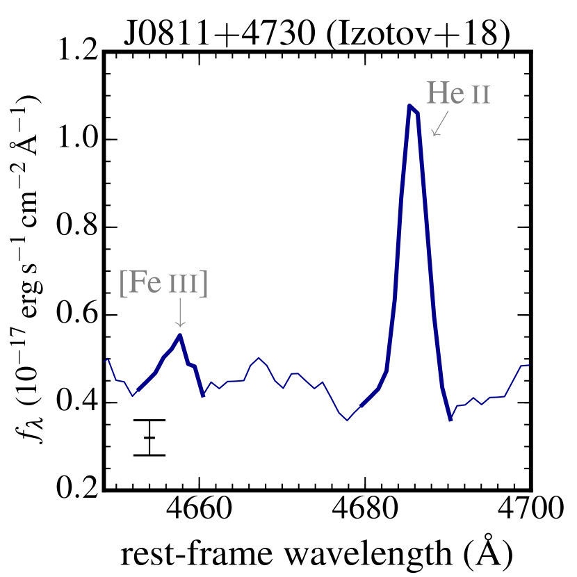
Figure 2.— Spectrum of J0811$+$4730 (Izotov et al., 2018) around the [Fe iii]4658 and He ii4686 emission lines. This spectrum was taken with Multi-Object Double Spectrographs (MODS) installed on Large Binocular Telescope (LBT). This spectrum is adapted from Izotov et al. (2018) with permission. The emission lines of [Fe iii]4658 and He ii4686 are detected with S/N$=$5.1 and S/N$=$14.9, respectively. Continuum is detected at S/N$\sim$10 (in private communication). The bar at the bottom left represents a typical error of the spectrum.

4. ANALYSIS

In this section, we explain the emission line measurement (Section 4.1) and the estimation of galaxy properties (Section 4.2) for our 10 metal-poor galaxies. Here we estimate stellar masses, star-formation rates, emission-line equivalent widths, sizes, and metallicities of our 10 metal-poor galaxies.

4.1. Emission Line Measurements

We measure central wavelengths and emission-line fluxes with a best-fit gaussian profile using the iraf routine, splot. We also estimate flux errors, which originate from read-out noise and photon noise of sky$+$object emission. As described in Section 3.2, we correct fluxes of the LDSS-3/MagE spectra assuming the wavelength-dependent slit-loss with the model of the atmospheric refraction. We measure observed-frame equivalent widths (EWs) of emission lines with the same iraf routine, splot and convert them into the rest-frame equivalent widths (EW₀). Redshifts are estimated by comparing the observed central wavelengths and the rest-frame wavelengths in the air of strong emission lines.

Color excesses, $E$($B$$-$$V$) are estimated with the Balmer decrement of H$\alpha$, H$\beta$, H$\gamma$, H$\delta$,…, and H13 lines under the assumptions of the dust extinction curve given by Cardelli et al. (1989) and the case B recombination. We do not use Balmer emission lines affected by a systematic error such as cosmic rays and other emission lines blending with the Balmer line. In the case B recombination, we carefully assume electron temperatures ($T_{\mathrm{e}}$) so that the assumed electron temperatures become consistent with electron temperature measurements of O²⁺, $T_{\mathrm{e}}$(O iii), which will be obtained in Section 4.2. We estimate the best $E$($B$$-$$V$) values and their errors with the $\chi^{2}$ method (Press et al., 2007). The $E$($B$$-$$V$) estimation process is detailed in Paper I. We eventually assume $T_{e}$=10,000 K (SDSS J0002$+$1715 and SDSS J1642$+$2233), 15,000 K (HSC J1429$-$0110, HSC J2314$+$0154, SDSS J2253$+$1116, SDSS J2310$-$0211, and SDSS J2327$-$0200), 20,000 K (HSC J1142$-$0038 and SDSS J2115$-$1734), 25,000 K (HSC J1631$+$4426), which are roughly consistent with $T_{\mathrm{e}}$(O iii) measurements. We summarize the dust-corrected fluxes in Table 1.

Table 1Flux measurements

#	ID	[O ii]3727	[O ii]3729	[O ii]tot	H13	H12	H11	H10	H9
(1)	(2)	(3)	(4)	(5)	(6)	(7)	(8)	(9)	(10)
1	HSC J1429$-$0110	—	—	166.62$\pm$1.99	—	—	—	—	5.45$\pm$0.68
2	HSC J2314$+$0154	$<$14.21	$<$13.50	$<$19.60	—	—	—	—	—
3	HSC J1142$-$0038	68.06$\pm$0.81	91.82$\pm$0.84	159.88$\pm$1.16	3.26$\pm$0.68	3.63$\pm$0.67	6.65$\pm$0.79	4.39$\pm$0.66	6.13$\pm$0.63
4	HSC J1631$+$4426	—	—	50.12$\pm$2.66	—	—	—	—	4.68$\pm$1.17
5	SDSS J0002$+$1715	74.28$\pm$0.50	103.08$\pm$0.51	177.36$\pm$0.71	—	—	—	5.99$\pm$0.30	8.42$\pm$0.25
6	SDSS J1642$+$2233	103.35$\pm$0.72	149.41$\pm$0.76	252.75$\pm$1.05	—	—	—	—	6.74$\pm$0.33
7	SDSS J2115$-$1734	34.05$\pm$0.27	46.85$\pm$0.30	80.91$\pm$0.41	2.80$\pm$0.20	3.42$\pm$0.32	4.23$\pm$0.20	4.40$\pm$0.19	5.88$\pm$0.18
8	SDSS J2253$+$1116	39.44$\pm$0.11	55.06$\pm$0.12	94.50$\pm$0.16	2.36$\pm$0.06	3.40$\pm$0.05	4.08$\pm$0.05	5.59$\pm$0.05	7.59$\pm$0.05
9	SDSS J2310$-$0211	43.70$\pm$0.10	59.12$\pm$0.12	102.82$\pm$0.16	2.38$\pm$0.06	2.75$\pm$0.06	3.78$\pm$0.06	5.72$\pm$0.07	7.49$\pm$0.06
10	SDSS J2327$-$0200	45.07$\pm$0.11	59.96$\pm$0.12	105.03$\pm$0.16	2.48$\pm$0.06	3.36$\pm$0.06	3.99$\pm$0.08	5.29$\pm$0.06	7.19$\pm$0.06
#	[Ne iii]3869	[Ne iii]3967	H7	H$\delta$	H$\gamma$	[O iii]4363	[Fe iii]4658	HeII4686	[Ar iv]4711
(1)	(11)	(12)	(13)	(14)	(15)	(16)	(17)	(18)	(19)
1	63.97$\pm$0.70	—	32.48$\pm$0.48 a	21.64$\pm$0.33	45.55$\pm$0.28	9.06$\pm$0.23	0.94$\pm$0.17	1.36$\pm$0.17	2.02$\pm$0.16
2	$<$5.87	$<$3.90	—	26.15$\pm$3.11	46.56$\pm$1.67	$<$1.61	$<$1.15	$<$1.04	$<$0.94
3	29.33$\pm$0.63	7.74$\pm$0.54	17.16$\pm$0.54	27.36$\pm$0.51	48.20$\pm$0.43	5.96$\pm$0.39	$<$0.29	$<$0.30	$<$0.41
4	21.73$\pm$1.11	—	20.03$\pm$0.87 a	27.53$\pm$0.65	46.88$\pm$0.50	8.18$\pm$0.48	0.92$\pm$0.38	2.32$\pm$0.38	$<$0.35
5	46.64$\pm$0.30	15.00$\pm$0.21	16.27$\pm$0.19	26.04$\pm$0.17	46.92$\pm$0.14	6.38$\pm$0.09	0.66$\pm$0.05	0.86$\pm$0.05	0.79$\pm$0.06
6	44.64$\pm$0.37	12.19$\pm$0.25	15.27$\pm$0.24	26.44$\pm$0.20	44.90$\pm$0.16	6.59$\pm$0.10	0.65$\pm$0.06	1.20$\pm$0.06	0.44$\pm$0.11
7	43.59$\pm$0.24	13.97$\pm$0.17	15.54$\pm$0.16	26.12$\pm$0.16	46.99$\pm$0.16	13.94$\pm$0.11	0.87$\pm$0.06	2.67$\pm$0.11	1.89$\pm$0.08
8	64.12$\pm$0.11	18.82$\pm$0.06	16.12$\pm$0.06	25.67$\pm$0.05	46.52$\pm$0.06	14.13$\pm$0.04	0.36$\pm$0.01	0.30$\pm$0.02	2.12$\pm$0.02
9	53.54$\pm$0.10	15.86$\pm$0.06	16.38$\pm$0.06	26.66$\pm$0.06	48.57$\pm$0.07	14.85$\pm$0.04	0.45$\pm$0.02	0.48$\pm$0.02	1.70$\pm$0.02
10	50.72$\pm$0.11	15.14$\pm$0.07	17.45$\pm$0.07	25.93$\pm$0.07	47.39$\pm$0.08	12.81$\pm$0.05	0.63$\pm$0.03	0.78$\pm$0.03	1.51$\pm$0.03

Note. — (1): Number. (2): ID. (3)–(36): Dust-corrected emission-line fluxes normalized to an H$\beta$ line flux in the unit of erg s^-1 cm^-2. Upper limits are given with a 1$\sigma$ level. Lines suffering from saturation or affected by sky emission lines are shown as no data here. [O ii]_tot represents a sum of [O ii]3727 and [O ii]3729 fluxes. If the spectral resolution is not high enough to resolve [O ii]3727 and [O ii]3729 lines, we only show [O ii]_tot fluxes.

Table 1Flux measurements — Continued

#	ID	[Ar iv]4740	H$\beta$	[O iii]4959	[O iii]5007	HeI5876	[O i]6300	[S iii]6312	[N ii]6548
(1)	(2)	(20)	(21)	(22)	(23)	(24)	(25)	(26)	(27)
1	HSC J1429$-$0110	0.96$\pm$0.16	100.00$\pm$0.24	210.62$\pm$0.29	626.89$\pm$0.46	9.28$\pm$0.09	2.94$\pm$0.08	1.07$\pm$0.08	$<$0.19
2	HSC J2314$+$0154	$<$1.01	100.00$\pm$1.00	69.57$\pm$0.72	207.48$\pm$0.88	12.85$\pm$0.41	11.88$\pm$0.48	$<$0.44	$<$0.32
3	HSC J1142$-$0038	$<$0.36	100.00$\pm$0.52	102.76$\pm$0.47	308.14$\pm$0.65	11.11$\pm$0.31	5.29$\pm$0.31	$<$0.30	1.99$\pm$0.24
4	HSC J1631$+$4426	$<$0.36	100.00$\pm$0.37	55.76$\pm$0.34	170.92$\pm$0.38	9.12$\pm$0.60	—	$<$0.55	$<$0.50
5	SDSS J0002$+$1715	0.88$\pm$0.06	100.00$\pm$0.16	196.65$\pm$0.19	593.18$\pm$0.32	11.09$\pm$0.05	2.34$\pm$0.04	1.63$\pm$0.03	1.92$\pm$0.03
6	SDSS J1642$+$2233	0.78$\pm$0.07	100.00$\pm$0.17	183.24$\pm$0.21	571.59$\pm$0.34	10.74$\pm$0.06	2.59$\pm$0.04	1.88$\pm$0.04	1.68$\pm$0.04
7	SDSS J2115$-$1734	1.75$\pm$0.07	100.00$\pm$0.19	165.47$\pm$0.22	—	10.80$\pm$0.06	1.70$\pm$0.05	1.71$\pm$0.05	1.18$\pm$0.04
8	SDSS J2253$+$1116	1.69$\pm$0.02	100.00$\pm$0.07	250.60$\pm$0.11	—	11.17$\pm$0.02	—	—	1.16$\pm$0.01
9	SDSS J2310$-$0211	1.40$\pm$0.02	100.00$\pm$0.09	214.32$\pm$0.12	—	10.41$\pm$0.03	2.39$\pm$0.02	1.23$\pm$0.02	1.07$\pm$0.02
10	SDSS J2327$-$0200	1.12$\pm$0.03	100.00$\pm$0.11	200.95$\pm$0.14	—	11.28$\pm$0.04	2.79$\pm$0.03	1.52$\pm$0.02	1.31$\pm$0.02
#	H$\alpha$	[N ii]6584	HeI6678	[S ii]6716	[S ii]6731	HeI7065	[Ar iii]7136	[O ii]7320	[O ii]7330
(1)	(28)	(29)	(30)	(31)	(32)	(33)	(34)	(35)	(36)
1	246.66$\pm$0.20	5.08$\pm$0.18	2.96$\pm$0.07	7.87$\pm$0.08	6.07$\pm$0.08	2.73$\pm$0.07	5.62$\pm$0.08	1.45$\pm$0.07	0.92$\pm$0.07
2	278.45$\pm$0.66	2.10$\pm$0.29	—	5.18$\pm$0.33	$<$0.55	—	$<$0.85	$<$0.46	$<$0.61
3	272.09$\pm$0.57	8.64$\pm$0.26	2.75$\pm$0.21	16.24$\pm$0.24	8.52$\pm$0.27	$<$0.30	5.52$\pm$0.43	$<$0.36	$<$0.37
4	229.46$\pm$1.00	$<$0.48	2.07$\pm$0.59	—	—	—	—	$<$0.48	$<$0.54
5	280.48$\pm$0.17	5.68$\pm$0.04	2.99$\pm$0.03	11.19$\pm$0.04	5.97$\pm$0.03	2.58$\pm$0.03	—	—	—
6	276.34$\pm$0.20	5.28$\pm$0.04	2.64$\pm$0.03	10.39$\pm$0.06	8.14$\pm$0.04	1.42$\pm$0.04	6.30$\pm$0.05	1.84$\pm$0.04	1.47$\pm$0.04
7	278.90$\pm$0.22	3.11$\pm$0.04	—	5.23$\pm$0.04	4.66$\pm$0.04	3.61$\pm$0.05	4.61$\pm$0.06	1.09$\pm$0.04	0.83$\pm$0.04
8	—	3.29$\pm$0.01	2.97$\pm$0.01	6.47$\pm$0.01	5.07$\pm$0.01	3.56$\pm$0.01	5.08$\pm$0.02	1.55$\pm$0.01	1.03$\pm$0.01
9	—	2.76$\pm$0.02	2.65$\pm$0.02	7.65$\pm$0.02	5.56$\pm$0.02	3.18$\pm$0.02	4.70$\pm$0.02	1.26$\pm$0.02	0.98$\pm$0.02
10	—	3.21$\pm$0.02	2.93$\pm$0.02	8.78$\pm$0.03	6.49$\pm$0.03	3.83$\pm$0.03	5.36$\pm$0.03	1.69$\pm$0.02	—

Note. — Continued.

Table 2Parameters of our metal-poor galaxies

#	ID	EMPG?	redshift	$\textrm{EW}_{0}$(H$\beta$)	12+log(O/H)	$\log$($M_{\star}$)	$\log$($SFR$)	$E$($B$$-$$V$)
				(Å)		($M_{\odot}$)	($M_{\odot}$ yr-1)	(mag)
(1)	(2)	(3)	(4)	(5)	(6)	(7)	(8)	(9)
1	HSC J1429$-$0110	no	$0.02980$	$172.6^{+0.7}_{-0.6}$	$8.27\pm 0.02$	$6.55^{+0.13}_{-0.09}$	$0.43\pm 0.01$	$0.35\pm 0.02$
2	HSC J2314$+$0154	yesa	$0.03265$	$213.3^{+23.4}_{-17.6}$	$7.23^{+0.03}_{-0.02}$a	$5.17\pm 0.01$	$-0.85\pm 0.01$	$0.28\pm 0.03$
3	HSC J1142$-$0038	no	$0.02035$	$111.9^{+1.4}_{-1.3}$	$7.72\pm 0.03$	$4.95^{+0.04}_{-0.01}$	$-1.07\pm 0.01$	$0.00^{+0.02}_{-0.00}$
4	HSC J1631$+$4426	yes	$0.03125$	$123.5^{+3.5}_{-2.8}$	$6.90\pm 0.03$	$5.89^{+0.10}_{-0.09}$	$-1.28\pm 0.01$	$0.19\pm 0.03$
5	SDSS J0002$+$1715	no	$0.02083$	$103.9\pm 0.2$	$8.22\pm 0.01$	$7.06\pm 0.03$	$0.00\pm 0.01$	$0.00^{+0.01}_{-0.00}$
6	SDSS J1642$+$2233	no	$0.01725$	$153.7^{+0.5}_{-0.4}$	$8.45\pm 0.01$	$6.06^{+0.03}_{-0.13}$	$-0.17\pm 0.01$	$0.02\pm 0.02$
7	SDSS J2115$-$1734	yes	$0.02296$	$214.0^{+0.9}_{-0.8}$	$7.68\pm 0.01$	$6.56\pm 0.02$	$0.27\pm 0.01$	$0.19\pm 0.03$
8	SDSS J2253$+$1116	no	$0.00730$	$264.7\pm 0.3$	$7.973\pm 0.002$	$5.78\pm 0.01$	$-0.54\pm 0.01$	$0.00^{+0.01}_{-0.00}$
9	SDSS J2310$-$0211	no	$0.01245$	$127.6\pm 0.2$	$7.890^{+0.003}_{-0.004}$	$6.99\pm 0.03$	$-0.16\pm 0.01$	$0.01^{+0.02}_{-0.01}$
10	SDSS J2327$-$0200	no	$0.01812$	$111.0\pm 0.2$	$7.866^{+0.004}_{-0.005}$	$6.51^{+0.02}_{-0.03}$	$-0.18\pm 0.01$	$0.00^{+0.02}_{-0.00}$

Note. — (1): Number. (2): ID. (3): Whether or not an object satisfies the EMPG definition, $12$+$\log({\rm O/H})$$<$7.69. If yes (no), we write yes (no) in the column. (5): Rest-frame equivalent width of an H$\beta$ emission line. (6): Gas-phase metallicity based on the $T_{\mathrm{e}}$ method except for HSC J2314$+$0154. (7): Stellar mass. (8): Star-formation rate. (9): Color excess.

4.2. Galaxy Properties

In this section, we estimate gas-phase metallicities (O/H), and gas-phase element abundance ratios of our 10 galaxies. Note that metallicities are already estimated in Paper I, as well as stellar masses, SFRs, and color excesses.

We estimate electron temperatures of O²⁺ ($T_{\mathrm{e}}$(Oiii)) and O⁺ ($T_{\mathrm{e}}$(Oii)), using line ratios of [O iii]4363/5007 and [O ii](3727+3729)/(7320+7330), respectively. We use nebular physics calculation codes of PyNeb (Luridiana et al., 2015, v1.0.14) to estimate electron temperatures. If an [O ii]5007 line is saturated, we estimate an [O ii]5007 flux with

$$\textrm{[O\,{iii}]}5007=2.98\times\textrm{[O\,{iii}]}4959,$$ (1)

which is strictly determined by the Einstein A coefficient. If either of [O ii]7320 or [O ii]7330 line is detected, we estimate a total flux of [O ii](7320+7330) with a relation of

$$\textrm{[O\,{ii}]}7330=0.56\times\textrm{[O\,{ii}]}7320.$$ (2)

We have confirmed that Equation (2) holds with very little dependence on $T_{\mathrm{e}}$ and $n_{\mathrm{e}}$, using PyNeb. If none of [O ii]7320,7330 line is detected, we estimate $T_{\mathrm{e}}$(Oii) from an empirical relation of

$${T_{\mathrm{e}}}(\textrm{O\,{ii}})=0.7\times{T_{\mathrm{e}}}(\textrm{O\,{iii}})+3000,$$ (3)

which has been confirmed by Campbell et al. (1986) and Garnett (1992). We also assume

$${T_{\mathrm{e}}}(\textrm{S\,{iii}})=0.83\times{T_{\mathrm{e}}}(\textrm{O\,{iii}})+1700,$$ (4)

to estimate electron temperatures associated with S²⁺ ions (Garnett, 1992). We regard $T_{\mathrm{e}}$(Oiii), $T_{\mathrm{e}}$(Siii), and $T_{\mathrm{e}}$(Oii) as representative electron temperatures associated with ions in high, intermediate, and low ionization states, respectively.

We estimate gas-phase metallicities, $12$+$\log({\rm O/H})$, based on electron temperature measurements, which are so-called $T_{\mathrm{e}}$-metallicities. Hereafter, we call the $T_{\mathrm{e}}$-metallicity just “metallicity” unless we describe explicitly. We also use PyNeb to estimate metallicities. The latest atomic data are used in the PyNeb codes. We do not estimate a $T_{\mathrm{e}}$-based metallicity of HSC J2314$+$0154 because none of the $T_{\mathrm{e}}$(Oiii), $T_{\mathrm{e}}$(Oii), and $T_{\mathrm{e}}$(Siii) is estimated due to non-detection of [O iii]4363 and [O ii]7320,7330 emission lines. Instead, we estimate the metallicity of HSC J2314$+$0154 with a calibrator obtained by Skillman (1989) as described in Paper I. The estimates of gas-phase metallicities are summarized in Table 2. The estimation of electron temperatures and metallicities are detailed in Paper I.

Table 3Element abundance ratios

#	ID	log(Ne/O)	log(Ar/O)	log(N/O)	log(Fe/O)
(1)	(2)	(3)	(4)	(5)	(6)
1	HSC J1429$-$0110	$-0.634^{+0.006}_{-0.007}$	$-2.634^{+0.028}_{-0.026}$	$-1.753^{+0.020}_{-0.023}$	$-1.994^{+0.091}_{-0.075}$-0.223c
2	HSC J2314$+$0154	— a	— a	— a	— a
3	HSC J1142$-$0038	$-0.712^{+0.008}_{-0.010}$	$<-2.253$	$-1.297^{+0.019}_{-0.014}$	$<-2.124$
4	HSC J1631$+$4426	$-0.641^{+0.022}_{-0.019}$	— b	$<-1.710$	$-1.246^{+0.174}_{-0.313}$-0.222c
5	SDSS J0002$+$1715	$-0.701^{+0.003}_{-0.002}$	— b	$-1.644\pm 0.004$	$-2.126^{+0.035}_{-0.027}$-0.217c
6	SDSS J1642$+$2233	$-0.754\pm 0.005$	$-2.704^{+0.016}_{-0.015}$	$-1.943^{+0.006}_{-0.009}$	$-2.335^{+0.027}_{-0.038}$-0.211c
7	SDSS J2115$-$1734	$-0.757^{+0.005}_{-0.004}$	$-2.274^{+0.007}_{-0.013}$	$-1.518^{+0.009}_{-0.011}$	$-1.639^{+0.026}_{+0.026}$-0.209c
8	SDSS J2253$+$1116	$-0.707\pm 0.001$	$-2.391\pm 0.002$	$-1.563\pm 0.003$	$-2.078^{+0.020}_{-0.022}$-0.221c
9	SDSS J2310$-$0211	$-0.761\pm 0.001$	$-2.440\pm 0.004$	$-1.710^{+0.005}_{-0.004}$	$-2.046^{+0.019}_{-0.023}$-0.210c
10	SDSS J2327$-$0200	$-0.737^{+0.001}_{-0.002}$	$-2.386\pm 0.006$	$-1.616^{+0.006}_{-0.004}$	$-1.890^{+0.022}_{-0.017}$-0.213c

Note. — (1): Number. (2): ID. (3)–(6): Gas-phase element abundance ratios of Ne/O, Ar/O, N/O, and Fe/O. Upper limits are given with a 2$\sigma$ confidence level.

We estimate gas-phase element abundance ratios of neon-to-oxygen (Ne/O), argon-to-oxygen (Ar/O), nitrogen-to-oxygen (N/O), and iron-to-oxygen (Fe/O) in a similar way to Izotov et al. (2006b). First, we estimate ion abundance ratios of Ne²⁺/H⁺, Ar³⁺/H⁺, Ar²⁺/H⁺, N⁺/H⁺, and, Fe²⁺/H⁺ with the PyNeb codes. The atomic data used in the PyNeb calculation are shown in Table 4. Because different ions reside in different parts of an H ii region, we choose one of the $T_{\mathrm{e}}$(Oiii), $T_{\mathrm{e}}$(Siii), and $T_{\mathrm{e}}$(Oii) to estimate abundances of each ion according to their ionization potential. We use $T_{\mathrm{e}}$(Oiii) to estimate abundances of O²⁺, Ne²⁺, and Ar³⁺. We adopt $T_{\mathrm{e}}$(Siii) in the estimation of Ar²⁺ abundances. We apply $T_{\mathrm{e}}$(Oii) for abundances of low-ionizion ions, O⁺, N⁺, and Fe²⁺. Second, we convert the ion abundances into element abundances with ionization correction factors ($ICF$s) of Izotov et al. (2006b) shown below:

$$\frac{\mathrm{Ne}}{\mathrm{H}} = \frac{\mathrm{Ne}^{+}}{\mathrm{H}^{+}}+ICF(\mathrm{Ne}^{+}),$$ (5)

$$\frac{\mathrm{Ar}}{\mathrm{H}} = \frac{\mathrm{Ar}^{3+}+\mathrm{Ar}^{2+}}{\mathrm{H}^{+}}+ICF(\mathrm{Ar}^{3+}+\mathrm{Ar}^{2+}),$$ (6)

$$\frac{\mathrm{N}}{\mathrm{H}} = \frac{\mathrm{N}^{+}}{\mathrm{H}^{+}}+ICF(\mathrm{N}^{+}),$$ (7)

$$\frac{\mathrm{Fe}}{\mathrm{H}} = \frac{\mathrm{Fe}^{2+}}{\mathrm{H}^{+}}+ICF(\mathrm{Fe}^{2+}).$$ (8)

The $ICF$s are based on H ii region models (Stasińska & Izotov, 2003) and are given as a function of $v=$O⁺/(O²⁺+O⁺) or $w=$O²⁺/(O²⁺+O⁺). Finally, we obtain Ne/O, Ar/O, N/O, and Fe/O ratios by dividing Ne/H, Ar/H, N/H, and Fe/H by O/H (i.e., metallicity). We do not estimate Ne/O, Ar/O, N/O, and Fe/O ratios of HSC J2314$+$0154 because none of the $T_{\mathrm{e}}$(Oiii), $T_{\mathrm{e}}$(Oii), and $T_{\mathrm{e}}$(Siii) is obtained. The Ar/O ratios of HSC J1631$+$4426 and SDSS J0002$+$1715 are not estimated as well because the [Ar iii]7136 emission line is strongly affected by the sky emission line. Rodriguez (2003) suggests that $ICF$(Fe²⁺) of the Stasińska & Izotov (2003) models may include systematic errors, which originate from uncertainties of a recombination rate of Fe²⁺ and/or uncertain collision strengths of Fe²⁺ and Fe³⁺. Thus, we also estimate the $ICF$(Fe²⁺) values with another model of Rodriguez & Rubin (2005). The ICFs obtained by the Stasińska & Izotov (2003) models are $\sim$0.2 dex higher than the Rodriguez & Rubin (2005) models. In this paper, we regard the ICF offsets between the two models as systematic errors of Fe/O, which are included in lower errors of Fe/O (see Table 3 and Figures 3 and 4). For the literature EMPG, J0811$+$4730, we derive the element abundances from Izotov et al. (2018). The element abundances of J0811$+$4730 are obtained in the same manner as in this paper. We summarize the element abundance ratios in Table 3.

Table 4Atomic Data

Ion	Emission Process	Atomic Data	Line Data
(1)	(2)	(3)	(4)
H0	Re	Storey & Hummer (1995)	Storey & Hummer (1995)
O+	CE	Fischer & Tachiev (2004)	Kisielius et al. (2009)
O2+	CE	Storey & Zeippen (2000), Fischer & Tachiev (2004)	Storey et al. (2014)
Ne2+	CE	Galavís et al. (1997)	McLaughlin & Bell (2000)
Ar2+	CE	Munoz Burgos et al. (2009)	Munoz Burgos et al. (2009)
Ar3+	CE	Mendoza & Zeippen (1982)	Ramsbottom & Bell (1997)
N+	CE	Fischer & Tachiev (2004)	Tayal (2011)
Fe2+	CE	Quinet (1996), Johansson et al. (2000)	Quinet (1996)

Note. — (1): Ion. (2): Re and CE represent the recombination and the collisional excitation, respectively. (3): References of transition probabilities used in this paper. (4): References of line emissivities in a 2D temperature-density dependent table (Re) and the temperature-dependent collision strengths (CE) applied in this paper.

5. RESULTS AND DISCUSSIONS

5.1. Element Abundance Ratios

We show the element abundance ratios of neon, argon, nitrogen, and iron to oxygen (Ne/O, Ar/O, N/O, and Fe/O) of our metal-poor galaxy sample consisting of 10 metal-poor galaxies from Paper I and J0811$+$4730 from Izotov et al. (2018). Figure 3 shows the Ne/O, Ar/O, N/O, and Fe/O ratios as a function of metallicity, 12+log(O/H). Thanks to the two representative EMPGs, HSC J1631$+$4426 (0.016 $Z_{\odot}$) and J0811$+$4730 (0.019 $Z_{\odot}$), we are able to investigate and discuss the low metallicity end (below 0.02 $Z_{\odot}$) of the element abundances for the first time. We discuss these element abundance ratios in the following subsections. We compare the element abundance ratios of our metal-poor galaxy sample with a metal-poor galaxy sample of Izotov et al. (2006b), whose typical stellar mass range is larger than our sample galaxies.

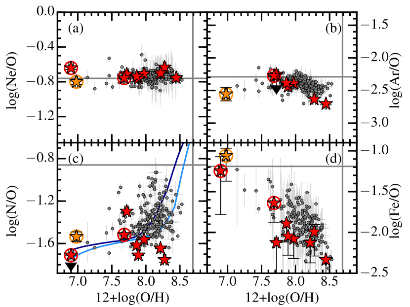
Figure 3.— Element abundance ratios of neon, argon, nitrogen, and iron to oxygen (Ne/O, Ar/O, N/O, and Fe/O) are shown as a function of metallicity in the panels (a) to (d), respectively. Our metal-poor galaxies from HSC-EMPG and SDSS-EMPG source catalogs are shown with red stars. The EMPG, J0811$+$4730, which is derived from Izotov et al. (2018) is shown with the orange star. Metal-poor galaxies that satisfy the EMPG are marked with a large circle. Here we do not show HSC J2314$+$0154, whose $T_{\mathrm{e}}$-metallicity and element abundances are not estimated due to the lack of the electron temperature measurement. Gray dots represent local galaxies of Izotov et al. (2006b). Gray vertical and horizontal lines indicate solar abundance ratios and metallicity (Asplund et al., 2009). Solid lines in the panel (c) are the model calculations of the N/O evolution (Vincenzo et al., 2016) with star-formation efficiencies of 0.5 (dark blue) and 1.0 (light blue) Gyr^-1. The Ar/O ratios of HSC J1631$+$4426 and SDSS J0002$+$1715 are not shown here because the [Ar iii]7136 emission line is strongly affected by the sky emission line.

5.1.1 Ne/O and Ar/O ratios

Izotov et al. (2006b) report that Ne/O and Ar/O ratios little depend on metallicity because the neon, argon, and oxygen are all $\alpha$ elements, which are produced by the nuclear fusion of $\alpha$ particles inside stars. As shown in the panels (a) and (b) of Figure 3, we find that our metal-poor galaxy sample shows almost constant values of $\log$(Ne/O) $\sim$$-0.8$ and $\log$(Ar/O)$\sim$$-2.5$ within a scatter of $\pm$0.2 dex, which are almost consistent with the solar abundance ratios. We also find that the Ne/O and Ar/O ratios are consistent with those of local galaxies reported by Izotov et al. (2006b) within the scatter. The consistency suggests that our metal-poor galaxy sample also shows no metallicity dependence in Ne/O and Ar/O ratios.

Note that the Ar/O ratio might slightly decrease in the range of $12$+$\log({\rm O/H})$$\gtrsim$8.2 in our sample and the Izotov et al. (2006b) sample, in contrast to the Ne/O ratios. The Ar/O ratio is expected to be constant and consistent with the solar abundance, $\log$(Ar/O)_⊙$=$$-2.29$, because there seems to be no physical reason for the Ar/O (i.e., $\alpha$ element ratio) decrease at $12$+$\log({\rm O/H})$$\gtrsim$8.2. It may be explained by the underlying unknown systematics in the Ar/O estimation at $12$+$\log({\rm O/H})$$\gtrsim$8.2. We do not discuss it further in this paper because the Ar/O abundances at relatively higher metallicities are out of the scope of this paper.

5.1.2 N/O ratio

As suggested by previous studies (Pérez-Montero & Contini, 2009; Pérez-Montero et al., 2013; Andrews & Martini, 2013), N/O ratios of SFGs present a plateau at $\log$(N/O)$\sim$$-1.6$ in the range of $12$+$\log({\rm O/H})$$\lesssim$8.0 and a positive slope at higher metallicities as a function of metallicity. The panel (c) of Figure 3 presents model calculations of the N/O evolution (Vincenzo et al., 2016), which also show the plateau and positive slope. The plateau basically results from the primary nucleosynthesis of massive stars, while the positive slope is mainly attributed to the secondary nucleosynthesis of low- and intermediate-mass stars (e.g., Vincenzo et al., 2016). We briefly describe the two nitrogen production processes below.

• Primary nucleosynthesis: Inside a metal-poor star, protons are burned through the proton-proton ($p$-$p$) chain reaction, and little nitrogen is produced at this stage. Nitrogen elements are mainly produced after the formation of a heavy-element core (e.g., O and C) and ejected into ISM by SNe, for stars more massive than $\sim$8 $M_{\odot}$.

• Secondary nucleosynthesis: Metal-rich stars efficiently burn hydrogen through the carbon-nitrogen-oxygen (CNO) cycle, where nitrogen elements accumulate because ¹⁴N fusion (¹⁴N$+$$p$ $\rightarrow$ ¹⁵O$+$$\gamma$) is the slowest process in the CNO cycle. Then nitrogen is ejected through stellar winds during the asymptotic giant branch (AGB) phase, $\sim$1 Gyr after the birth of low- and intermediate-mass stars.

As shown in the panel (c) of Figure 3, most of our metal-poor galaxies have N/O ratios of $\log$(N/O)$<$$-1.5$ (i.e., less than $\sim$30 percent of the solar N/O ratio). Especially, HSC J1631$+$4426 has a strong, 2$\sigma$ upper limit of $\log$(N/O)$<$$-1.71$, and J0811$+$4730 show a low N/O ratio of $\log$(N/O)$=$$-1.53$. The N/O values of the two EMPGs (HSC J1631$+$4426 and J0811$+$4730) will be discussed again in Section 5.1.3. These low N/O ratios suggest that our metal-poor galaxies have not yet started the secondary nucleosynthesis due to their low metallicities and young stellar ages.

We also find several galaxies of our metal-poor galaxy sample have relatively low N/O ratios compared to the model lines of Vincenzo et al. (2016) and Izotov et al. (2006b) SFGs at $12$+$\log({\rm O/H})$$\sim$8.0. Vincenzo et al. (2016) find that the N/O plateau is lowered under the assumption of high sSFR or the top heavy initial mass function (IMF). Indeed, our metal-poor galaxy sample have high sSFRs ($\sim$300 Gyr^-1) compared to those of the Izotov et al. (2006b) SFGs ($\sim$1–10 Gyr^-1) because we aim to obtain galaxies with high sSFRs in this study. Thus, the N/O differences between our metal-poor galaxy sample and Izotov et al. (2006b) SFG sample are explained by the sample selection.

5.1.3 Fe/O ratio

In the panel (d) of Figure 3, we find that our metal-poor galaxies show a decreasing trend in Fe/O ratio as metallicity increases. The same decreasing Fe/O trend is found in a star-forming-galaxy sample of Izotov et al. (2006b). Most of our metal-poor galaxies have Fe/O ratios comparable to a star-forming-galaxy sample of Izotov et al. (2006b). Three EMPGs, HSC J1631$+$4426, SDSS J2115$-$1734, and J0811$+$4730 (encircled by a red or orange circle) show relatively high Fe/O ratios, log(Fe/O)$>$$-1.7$, among our metal-poor galaxies. Especially, we find that HSC J1631$+$4426 and J0811$+$4730, two of the lowest metallicity galaxies with 0.016 and 0.019 (O/H)_⊙, have high Fe/O ratios of log(Fe/O)$=$$-1.25^{+0.17}_{-0.53}$ and log(Fe/O)$=$$-1.06^{+0.09}_{-0.31}$, respectively, which are comparable to the solar Fe/O ratio, log(Fe/O)_⊙$=$$-1.19$. In this paper, we mainly focus on the two representative EMPGs, HSC J1631$+$4426 and J0811$+$4730, which interestingly show high Fe/O ratios. Note again that J0811$+$4730 is an EMPG reported by Izotov et al. (2018). Table 5 summarizes the Fe/O ratios and He ii4686/H$\beta$ ratios (discussed in Section 5.2.2) of the two representative EMPGs (HSC J1631$+$4426 and J0811$+$4730), which play an important role in this paper. We also show the fluxes of the two kew emission lines of [Fe iii]4658 and He ii4686 in Table 5.

Table 5Parameters of two representative EMPGs

ID	12+log(O/H)	log(Fe/O)	log(He ii/H$\beta$)	$F$([Fe iii])	$F$(He ii)	Ref.
				(erg s-1 cm-2)	(erg s-1 cm-2)
(1)	(2)	(3)	(4)	(5)	(6)	(7)
HSC J1631$+$4426	$6.90\pm 0.03$	$-1.25^{+0.17}_{-0.31}$-0.22a	$-1.58^{+0.07}_{-0.08}$	$12.0\pm 5.02$	$30.5\pm 5.04$	This paper
J0811$+$4730	$6.98\pm 0.02$	$-1.06^{+0.09}_{-0.09}$-0.22a	$-1.64\pm 0.03$	$6.55\pm 1.26$	$28.6\pm 1.89$	I18

Note. — (1): ID. (2): Gas-phase metallicity. (3): Abundance ratio of log(Fe/O). (4): Emission line ratio of log(He ii/H$\beta$). (5)–(6): Emission line fluxes of [Fe iii]4658 and He ii4686 in the unit of 10^-18 erg s^-1 cm^-2. (7): Reference. I18 represents Izotov et al. (2018).

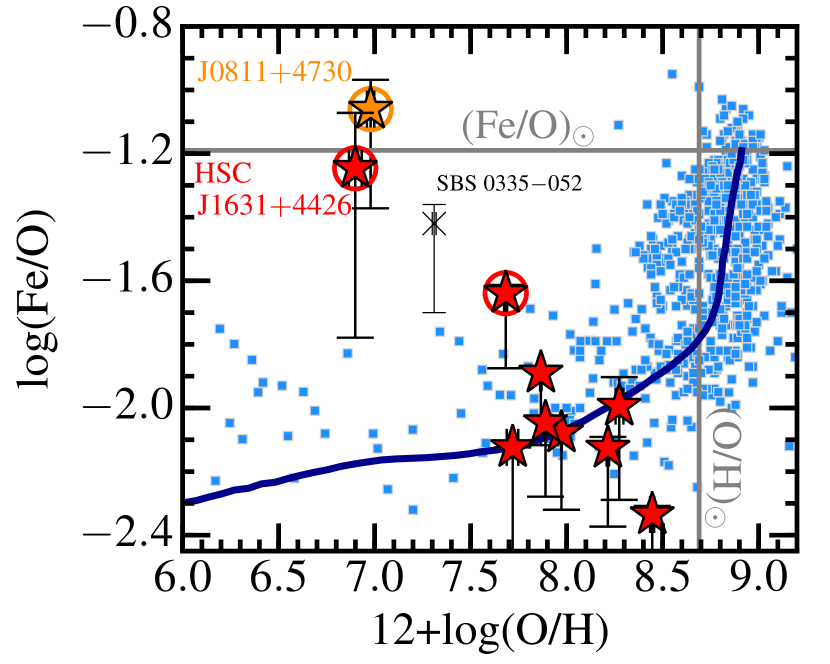
Figure 4.— Comparison of Fe/O ratios of our metal-poor galaxies (symbols are the same as Figure 3) and Galactic stars (blue squares). We show observational data of Galactic stars from Cayrel et al. (2004), Gratton et al. (2003), and Bensby et al. (2013). Blue solid line represents a stellar Fe/O evolution model under the assumption that gas is enriched by massive stars with 9–100 $M_{\odot}$ (Suzuki & Maeda, 2018). The cross represents another metal-poor galaxy, SBS 0335$-$052 from literature (Izotov & Thuan, 1999). SBS 0335$-$052 has 59% of the solar Fe/O ratio. Here we do not show HSC J2314$+$0154, whose $T_{\mathrm{e}}$-metallicity and element abundances are not estimated due to the lack of the electron temperature measurement.

To characterize the two EMPGs (HSC J1631$+$4426 and J0811$+$4730) with a high Fe/O ratio, we also compare our metal-poor galaxies with Galactic stars (Cayrel et al., 2004; Gratton et al., 2003; Bensby et al., 2013) in Figure 4. The Galactic star samples are composed of dwarf or subdwarf stars. The solid line here represents a stellar Fe/O evolution model under the assumption that gas is enriched by massive stars with 9–100 $M_{\odot}$ (Suzuki & Maeda, 2018). The gaseous abundance ratios at the time of the star formation are imprinted in the stellar abundance patterns because stars are formed from gas. As explained in Section 1, the Fe/O ratio increases at $12$+$\log({\rm O/H})$$\gtrsim$8.0 due to the contribution of type-Ia SNe $\sim$1 Gyr after the start of the star formation. Surprisingly, we find in Figure 4 that the two EMPGs (HSC J1631$+$4426 and J0811$+$4730) deviate from the observational results of Galactic stars and the Fe/O evolution model. Below, we mainly focus on the discussion of the two EMPGs of HSC J1631$+$4426 and J0811$+$4730, unless we specifically describe explicitly. Note that our metal-poor galaxies present gas-phase Fe/O ratios in nebulae, while the Galactic stars show the Fe/O ratio obtained from stellar atmospheric absorption lines. The nebular abundance ratios are subject to change by the effects of SNe, stellar wind, and galactic inflow in a short time scale (i.g., $\lesssim$ 10 Myr). By contrast, the abundance ratios of Galactic stars (i.e., dwarf and subdwarf stars) change little across the cosmic time because the element production proceeds very slowly and the heavy elements such as oxygen and iron are produced little in low-mass stars such as dwarf and subdwarf stars. Thus, the abundance ratios of the dwarf and subdwarf stars are almost fixed at the time of the star formation, and can be regarded as tracers of the past chemical evolution. The dwarf and subdwarf stars with low metallicities of 0.01–0.1 $Z_{\odot}$ are as old as $\sim$12 Gyr (e.g., Bensby et al., 2013), which is right after the MW formation. The two EMPGs (HSC J1631$+$4426 and J0811$+$4730), whose Fe/O ratios deviate from the Galactic stars and the Fe/O model, suggest that their Fe/O ratios have increased for some reason after the galaxy formation.

We discuss a possibility that the Fe/O ratios might be overestimated by the contribution of hard EUV radiation (e.g., AGNs) or shock heating (e.g., SNe). Collisional excitation lines of low-ionization ions such as [N ii], [S ii], and [Fe iii] are sensitive to hard EUV radiation or shock heating. For example, the strong [N ii]6584, [S ii]6717,6731 lines are often used in Baldwin-Phillips-Terlevich (BPT) diagram (Baldwin et al., 1981) as indicators of hard EUV radiation from an AGN. The AGN photoionization models (e.g., Groves et al., 2004a, b) actually predict [N ii] and [S ii] line intensities stronger than the stellar photoionization models. The [N ii] and [S ii] lines are enhanced by the power-law radiation of an AGN because a partially ionized zone is formed at the edge of ionized gas. In addition, shock gas models (Allen et al., 2008) also demonstrate that the [N ii] and [S ii] lines are boosted when the shock heating contributes to the line emission. The [N ii] and [S ii] lines are enhanced by the shock heating because low-ionization ions such as N⁺ and S⁺ are abundant in the recombination zone behind a shock front (Allen et al., 2008). Thus, abundances of low-ionization ions can be overestimated by the hard EUV radiation or shock heating. Especially, because the ionization potentials of N⁰ (14.5 eV) and Fe⁺ (16.2 eV) are very close, the N/O and Fe/O ratios can be overestimated simultaneously if the hard EUV radiation or shock heating contribute. However, the N/O ratios of the two EMPGs (HSC J1631$+$4426 and J0811$+$4730) are as low as galaxy chemical evolution models at $\log$(N/O)$\sim$$-1.6$. Only Fe/O ratios of the two EMPGs deviate from the chemical evolution models. Thus, we rule out the possibility that the Fe/O ratios are overestimated by the hard EUV radiation or shock heating.

We also discuss another possibility that the [Fe iii] 4658 emission line might be contaminated by a C iv 4659 emission line, which can lead to the overestimation of Fe/O ratio. If the C iv 4659 line exists, the [Fe iii] 4658 and C iv 4659 lines may be unresolved due to the low spectral resolutions of the FOCAS and MODS spectroscopy. The C iv 4659 line is a C³⁺ recombination line, which is characterized by stellar winds from Wolf-Rayet (WR) stars. Typical galaxies with WR features (so-called “WR galaxies”) show broad emission lines such as C iv 4659, He ii 4686, and C iv 5808 with FWHMs $\sim$ 3,000 km s^-1 (e.g., López-Sánchez & Esteban, 2010). Stellar wind velocities are expected to decrease with decreasing metallicity (e.g., Nugis & Lamers, 2000; Crowther & Hadfield, 2006) because atmospheric opacity of metal-poor stars becomes smaller than metal-rich stars. However, WR galaxies/stars at low metallicities are very rare and have not yet been studied very well. One of the most metal-poor galaxies, IZw 18 ($12$+$\log({\rm O/H})$$=$7.16, 0.030 $Z_{\odot}$) show prominent broad emission lines of C iv 4659, He ii 4686, and C iv 5808 with FWHMs $\sim$ 2,600–3,600 km s^-1 ($\Delta\lambda$$=$50–55Å, Legrand et al., 1997), which are as broad as typical metal-rich WR galaxies ($\sim$ 3,000 km s^-1, López-Sánchez & Esteban, 2010). The result may suggest that line widths of C iv 4659, He ii 4686, and C iv 5808 may be fairly large even when a galaxy has a few percent solar metallicity. In contrast to IZw 18, the two EMPGs discussed in this paper (HSC J1631$+$4426 and J0811$+$4730 with $\sim$0.02 $Z_{\odot}$) show no detection of broad emission lines of C iv 4659, He ii 4686, and C iv 5808. The detected [Fe iii] 4658 line of HSC J1631$+$4426 and J0811$+$4730 (FWHMs$\sim$4 Å, i.e., $\sim$ 260 km s^-1) are much narrower than the broad lines of IZw 18 (FWHMs $\sim$ 2,600–3,600 km s^-1). Thus, the C iv 4659 line originated from stellar winds may not contaminate the [Fe iii] 4658 line of HSC J1631$+$4426 and J0811$+$4730 significantly.

We briefly discuss an extreme case of a very narrow C iv 4659 line ($\lesssim$ 260 km s^-1), although the case is unlikely because the line width of $\lesssim$ 260 km s^-1 is one order of magnitude smaller than the the broad C iv 4659, He ii 4686, and C iv 5808 lines of IZw 18 (FWHMs $\sim$ 2,600–3,600 km s^-1). Even if the C iv 4659 line can be extremely narrow, non-detection of the C iv 5808 line suggests that the C iv 4659 line is very faint in HSC J1631$+$4426 and J0811$+$4730. Note that the C iv 5808 intensity is almost comparable to that of C iv 4659 (López-Sánchez & Esteban, 2010). Thus, we conclude that the [Fe iii] 4658 line is not contaminated by the C iv 4659 line significantly even in the extreme case.

As described above, we have found that the Fe/O ratios of the two EMPGs (HSC J1631$+$4426 and J0811$+$4730) deviate from the Galactic stars and the Fe/O chemical evolution models, and ruled out the possibility that the Fe/O ratios are overestimated. Below, we discuss three scenarios i)–iii) that might be able to explain the Fe/O deviation of the two EMPGs.

i) Preferential Dust Depletion: The first scenario is the preferential dust depletion of iron, suggested by Rodriguez & Rubin (2005) and Izotov et al. (2006b). Rodriguez & Rubin (2005) and Izotov et al. (2006b) explain that gas-phase Fe/O ratios decrease as a function of metallicity in the range of $12$+$\log({\rm O/H})$$\lesssim$8.5 because iron elements are depleted into dust more effectively than oxygen. The depletion becomes dominant in a higher metallicity range, where the dust production becomes more efficient. For dust-free (i.e., metal-poor) galaxies, gas-phase Fe/O ratios are expected to become comparable to the observational results of Galactic stars and the Fe/O evolution model. Although the dust depletion may explain the negative Fe/O slope, it does not explain the fact that the two EMPGs (HSC J1631$+$4426 and J0811$+$4730) show higher Fe/O ratios than the Galactic stars and models at fixed metallicity. In addition, as we have seen in Section 4.1 and Table 2, most of our metal-poor galaxies show $E$($B$$-$$V$)$\sim$0 (i.e., less dusty). At least, we do not find an evidence that galaxies with a larger metallicity show larger color excesses (i.e., dustier). This means that the Fe/O decrease of our sample is not attributed to the dust depletion. Based on these facts, we rule out the first scenario.

ii) Metal Enrichment and Gas Dilution: The second scenario is a combination of metal enrichment and gas dilution caused by inflow. In this scenario, we assume that EMPGs are formed from metal-enriched gas with the solar metallicity and solar Fe/O ratio. The Fe/O evolution models suggest that the Fe/O ratio increases at $12$+$\log({\rm O/H})$$\gtrsim$8.0 due to the contribution of type-Ia SNe $\sim$1 Gyr after the start of the star formation. Such mature galaxies also tend to have the solar metallicity (i.e, O/H) at the same time. If primordial gas (i.e., almost metal free) falls into the metal-enriched galaxies, the metallicity (i.e, O/H) decreases while the Fe/O ratio does not change. At first glance, this scenario seems to explain the Fe/O deviation of the two EMPGs. However, if the second scenario is true, both the Fe/O and N/O ratios should match solar abundances because the N/O ratio also reaches the solar N/O ratio, log(N/O)_⊙$=$$-0.86$, at the solar metallicity (Sections 1 and 5.1.2). As we have seen in the panel (c) of Figure 3, the two deviating EMPGs, HSC J1631$+$4426 and J0811$+$4730 (encircled by a red or orange circle at $12$+$\log({\rm O/H})$$\sim$7.0) have a strong 2$\sigma$ upper limit of $<$0.14 (N/O)_⊙ and a low value of 0.21 (N/O)_⊙, respectively. These low N/O ratios suggest that the two deviating EMPGs are experiencing the primary nucleosynthesis, not the secondary nucleosynthesis expected to start $\sim$1 Gyr after the onset of the star formation. This also means that the high Fe/O ratios are not attributed to the type-Ia SNe, which arise $\sim$1 Gyr after the onset of the star formation. This conclusion is also consistent with the fact that the two EMPGs are very young, $\lesssim 50$ Myr (Paper I). We exclude the second scenario because the second scenario does not explain the observed Fe/O and N/O ratios simultaneously.

iii) Super Massive Star Beyond 300 $M_{\odot}$: The third scenario is the contribution of super massive stars beyond 300 $M_{\odot}$. Super massive stars beyond 300 $M_{\odot}$ eject much iron at the time of core-collapse SN explosion. Ohkubo et al. (2006) have calculated yields from core-collapse SNe under the assumption of the progenitor stellar mass with 500–1000 $M_{\odot}$, obtaining $\sim$2–40 (Fe/O)_⊙. In the super massive stars beyond 300 $M_{\odot}$, an iron core grows until the iron core occupies more than 20 percent of the stellar mass. Although massive stars with 140–300 $M_{\odot}$ undergo thermonuclear explosions triggered by pair-creation instability (PISNe, Barkat et al., 1967), super massive stars beyond 300 $M_{\odot}$ are too massive to trigger PISNe and thus continue the iron core growth. The super massive stars beyond 300 $M_{\odot}$ eject a large amount of iron by a jet stream from the massive iron core during the SN explosion. On the other hand, the core-collapse SNe of typical-mass stars (10–50 $M_{\odot}$) eject gas with an average of $\sim$0.4 (Fe/O)_⊙ (Tominaga et al., 2007, IMF integrated in the range of 10–50 $M_{\odot}$), which is below the solar Fe/O ratio. Yields of type-Ia SNe calculated by Iwamoto et al. (1999) show $\sim$40 (Fe/O)_⊙. Of the three types of SNe, only the type-Ia SNe and the SNe of super massive stars ($>$300 $M_{\odot}$) contribute to the iron enrichment larger than the solar Fe/O ratio. As we have discussed in the second scenario above, the low N/O ratios of the two EMPGs suggest that their high Fe/O ratios are not explained by type-Ia SNe. Ruling out the type-Ia SNe, we find that the remaining possibility is the contribution from the SNe of super massive stars beyond 300 $M_{\odot}$. We also confirm that SNe of the super massive stars ($>$300 $M_{\odot}$) do not change N/O ratios in comparison with the core-collapse SNe of typical massive stars (Iwamoto et al., 1999; Ohkubo et al., 2006), strengthening the reliability of the super massive star ($>$300 $M_{\odot}$) scenario.

In addition to the two EMPGs (HSC J1631$+$4426 and J0811$+$4730) with $\sim$2% solar metallicity, a metal-poor galaxy, SBS 0335$-$052, shows $12$+$\log({\rm O/H})$$=$7.31$\pm$0.01 (i.e., 4.2% solar metallicity) and $\log$(Fe/O)$=$$-$1.42${}^{+0.06}_{-0.28}$, which is 59% of the solar Fe/O ratio (Izotov et al., 2006a). In Figure 4, SBS 0335$-$052 also deviates from the observational results of Galactic stars and the Fe/O evolution model, which supports the results of this paper. Note that Izotov & Thuan (1999) suggest that the Fe/O value of SBS 0335$-$052 can be overestimated by the C iv 4659 contamination on the [Fe iii] 4658 line, based on the low resolution spectroscopy of Multiple Mirror Telescope (MMT) spectrophotometry ($R$ $\sim$ 700). However, conducting the VLT/GIRAFFE spectroscopy with high spectral resolutions ($R$ $\sim$ 10,000), Izotov et al. (2006a) find that the [Fe iii] 4658 line is very narrow ($\sim$ 1 Å, i.e., $\sim$ 60 km s^-1), which is not explained by the C iv 4659 line originated from stellar winds. Non-detection of the C iv 5808 line also suggests that the C iv 4659 line is not strong enough to contaminate the [Fe iii] 4658 line significantly. Thus, SBS 0335$-$052 (Izotov et al., 2006a) is another example of a metal-poor galaxy that significantly shows a higher Fe/O ratio than the chemical evolution models. Izotov et al. (2006a) attribute the higher Fe/O ratio of SBS 0335$-$052 to low dust depletion of iron, which has been ruled out in this paper (i.e., the first scenario in this section).

In summary of this subsection, we have discussed the three scenarios that might be able to explain the high Fe/O ratios of the two EMPGs (HSC J1631$+$4426 and J0811$+$4730). We suggest that the high Fe/O ratios of the two EMPGs are attributed to the contribution from core-collapse SNe of super massive stars beyond 300 $M_{\odot}$. The contribution of super massive stars beyond 300 $M_{\odot}$ to the iron enhancement has never been discussed by previous studies including Izotov et al. (2006b) and Izotov et al. (2018). Many previous studies (e.g., Fragos et al., 2013a, b; Stanway et al., 2016; Suzuki & Maeda, 2018; Xiao et al., 2018) assume the IMF maximum stellar mass ($M_{\mathrm{max}}$) at $M_{\mathrm{max}}$$=$100, 120, or 300 $M_{\mathrm{\odot}}$, ignoring super massive stars beyond 300 $M_{\odot}$, so this paper sheds light on the super massive stars beyond 300 $M_{\odot}$ in metal-poor galaxies undergoing the early-phase galaxy formation.

5.2. Ionizing Radiation

5.2.1 Emission Line Ratios

We investigate ionizing radiation of our metal-poor galaxy sample by comparing emission line ratios of various ions. Figure 5 shows four emission line ratios of [O ii]3727,3729/H$\beta$, [Ar iii]4740/H$\beta$, [O iii]5007/H$\beta$, and [Ar iv]7136/H$\beta$ as a function of metallicity. Among many emission lines detected in our spectroscopy, we choose the [O ii]3727,3729, [Ar iii]4740, [O iii]5007, and [Ar iv]7136 emission lines for two reasons below. The first reason is that oxygen and argon are both $\alpha$ elements, and thus the Ar/O abundance ratio is almost constant as we confirm in Section 5.1. Thus, emission line ratios are simply interpreted by ionizing radiation intensity and/or hardness, free from variance of element abundance ratio. The second reason is that the four lines are sensitive to ionization photons in a wide energy range from 13.6 to 40.7 eV. The [O ii]3727,3729, [Ar iii]4740, [O iii]5007, and [Ar iv]7136 lines are emitted via spontaneous emission after collisional excitation of O⁺, Ar²⁺, O²⁺, and Ar³⁺, respectively. Table 6 summarizes these emission line processes and corresponding photon energy required to emit these lines.

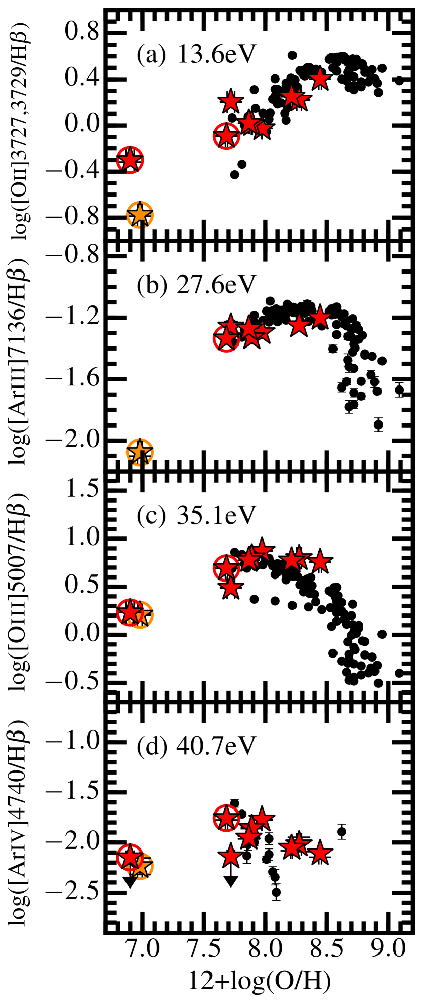
Figure 5.— Dust-corrected emission line ratios of [O ii]3727,3729, [Ar iii]4740, [O iii]5007, and [Ar iv]7136 to H$\beta$ in panels (a)–(d). Symbols are the same as in Figure 3. Here we do not show HSC J2314$+$0154 as well, whose $T_{\mathrm{e}}$-metallicity and element abundances are not estimated. The ionization potentials of O⁰, Ar²⁺, O⁺, and Ar³⁺ ions (13.6, 27.6, 35.1, and 40.7 eV, respectively) are presented in panels (a)–(d). Black circles represent averages of local SFGs obtained with SDSS composite spectra (Andrews & Martini, 2013). We do not show galaxies whose nebular emission line is strongly affected by the sky emission line.

Table 6Summary of Emission Line Process, Ionization Process and Ionization Potential

Line	Emission	Ionization	Ionization
	Process	Process	Potential
			(eV)
H$\beta$	Re	H0+$\gamma$ $\rightarrow$ H+	13.6
[O ii]3727	CE	O0+$\gamma$ $\rightarrow$ O+	13.6
[Ar iii]4740	CE	Ar2++$\gamma$ $\rightarrow$ Ar3+	27.6
[O iii]5007	CE	O++$\gamma$ $\rightarrow$ O2+	35.1
[Ar iv]7136	CE	Ar3++$\gamma$ $\rightarrow$ Ar4+	40.7
He ii4686	Re	He++$\gamma$ $\rightarrow$ He2+	54.4

Note. — In the column of emission processes, Re and CE represent the recombination and collisional excitation.

In panels of (a)–(d) of Figure 5, we show local, average SFGs of Andrews & Martini (2013, AM13 hereafter) with black circles. We regard the AM13 SFGs as local averages because the AM13 sample is obtained by the SDSS composite spectra in bins of wide SFR and stellar-mass ranges. In panels of (a)–(d), the AM13 SFGs form sequences as a function of metallicity. The sequences of [O ii]3727,3729/H$\beta$ and [Ar iii]4740/H$\beta$ show peaks at around $12$+$\log({\rm O/H})$$\sim$8.7 and 8.3, respectively. The [O iii]5007/H$\beta$ and [Ar iv]7136/H$\beta$ ratios may also have peaks around $12$+$\log({\rm O/H})$ $\sim$8.0 and $12$+$\log({\rm O/H})$$\sim$7.2–7.7 by interpolating AM13 SFGs and our metal-poor galaxies. Recalling that the [O ii]3727,3729, [O iii]5007, [Ar iii]4740, and [Ar iv]7136 lines are sensitive to ionizing photon above 13.6, 35.1, 27.6, and 40.7 eV, respectively, we find that the peak metallicities decrease with increasing ionizing potentials of the corresponding emission lines. The peak transition demonstrates that ISM is irradiated by more intense or harder ionizing radiation in lower metallicity, as suggested by previous studies (e.g., Nakajima & Ouchi, 2014; Steidel et al., 2016; Nakajima et al., 2016; Kojima et al., 2017). We also find that our metal-poor galaxies fall on the sequences of AM13 SFGs within a scatter. Thus, we infer that our metal-poor galaxies and the AM13 SFGs have a similar spectral shape in the energy range of 13.6–40.7 eV for a given metallicity.

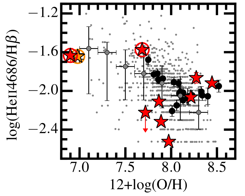
Figure 6.— Emission line ratios of He ii4686/H$\beta$ as functions of metallicity. Symbols are the same as in Figure 5. Here we do not show HSC J2314$+$0154, whose $T_{\mathrm{e}}$-metallicity and element abundances are not estimated. Gray dots are individual local galaxies of S19 with an He ii4686 detection. Gray circles and error bars show medians and 68%-percentile scatters of the S19 sample obtained in each metallicity bin, respectively.

Figure 6 shows He ii4686/H$\beta$ ratios of our metal-poor galaxies as a function of metallicity, as well as the AM13 SFGs (black circles). The AM13 SFGs show almost constant He ii4686/H$\beta$ ratios around log(He ii4686/H$\beta$)$\sim$$-2.0$ in the range of $12$+$\log({\rm O/H})$$=$8.1–8.6, while the He ii4686/H$\beta$ ratios increases with decreasing metallicity below $12$+$\log({\rm O/H})$$=$8.1. Our metal-poor galaxies show a wide range of He ii4686/H$\beta$ ratios between log(He ii4686/H$\beta$)$\sim$$-1.6$ and $-2.6$. The distribution of our metal-poor galaxies are similar to those of SFGs of Schaerer et al. (2019, S19 hereafter). Among our metal-poor galaxies, three EMPGs (encircled by red and orange circles) show highest He ii4686/H$\beta$ ratios around log(He ii4686/H$\beta$)$\sim$$-1.6$, including the two representative EMPGs, HSC J1631$+$4426 and J0811$+$4730 (Izotov et al., 2018).

As described in Section 1, previous studies also find large He ii4686/H$\beta$ ratios of $\log$(He ii4686/H$\beta$)$>$$-1.8$. In a study of WR galaxies, López-Sánchez & Esteban (2010) find 4 galaxies that show large He ii4686/H$\beta$ ratios of $\log$(He ii4686/H$\beta$)$=$$-1.7$ to $-1.5$ with no WR features in the metallicity range of $12$+$\log({\rm O/H})$$\sim$7.6–8.1. Shirazi & Brinchmann (2012) construct an SDSS galaxy sample with a He ii4686 detection. Shirazi & Brinchmann (2012) find 68 galaxies that have $\log$(He ii4686/H$\beta$)$=$$-2.4$ to $-1.8$ with no WR features in metallicity range of $12$+$\log({\rm O/H})$$\sim$7.7–8.2. Senchyna et al. (2017) conduct HST/COS spectroscopy for 5 SDSS galaxies with a nebular He ii4686 detection and no WR features. The 5 galaxies show $\log$(He ii4686/H$\beta$)$=$$-2.1$ to $-1.4$ in metallicity range of $12$+$\log({\rm O/H})$$\sim$7.8–8.0. Our EMPGs, HSC J1631$+$4426 and J0811$+$4730 have $12$+$\log({\rm O/H})$$\sim$6.90 and 6.98, respectively, which are much lower than those of these samples. The He ii4686/H$\beta$ ratios of HSC J1631$+$4426 and J0811$+$4730 are $\log$(He ii4686/H$\beta$)$\sim$$-1.6$, which is comparable to those of the three samples of López-Sánchez & Esteban (2010), Shirazi & Brinchmann (2012), and Senchyna et al. (2017).

5.2.2 Strong He ii4686 Line

As described in Section 1, the physical mechanism of the He ii4686 emission from SFGs is still under debate. One of possible sources of He⁺ ionizing photons is the very hot star produced via binary evolution. Xiao et al. (2018) have created nebular emission models with the combination of the photoionization code cloudy (Ferland et al., 2013) and the bpass code (Stanway et al., 2016; Eldridge et al., 2017). The bpass code calculates the stellar binary evolution, including atmosphere stripping, stellar rotation, and stellar mergers. The binary stellar evolution models of Xiao et al. (2018) predict low values of He ii4686/H$\beta$$\lesssim$1/1000, which are well below the observed He ii4686/H$\beta$ ratios of our galaxies and S19 galaxies (He ii4686/H$\beta$$\sim$1/300–1/30). This result suggests that the main contributors of He ii4686 are not hot stars produced via binary evolution themselves.

Another possible explanation is a high mass X-ray binary (HMXB), where X-ray is emitted from a binary system of a compact object and a star through gas accretion. S19 aim to explain the He ii4686 emission from local SFGs with HMXB models of Fragos et al. (2013a, b). HMXBs are binary systems consisting of a compact object (such as BH) and a companion star. The companion star provides gas onto the compact object, and creates a hot accretion disk around the compact object. The hot accretion disk radiates very hard, power-low radiation ranging from UV to X-ray. Fragos et al. (2013a, b) carefully calculate the HMXB evolution along the star-formation history, and predict total X-ray luminosities ($L_{\mathrm{X}}$) from a galaxy as functions of metallicity and age. S19 convert an $L_{\mathrm{X}}$/SFR ratio to the He ii4686/H$\beta$ ratio, under the simple assumptions of He ii4686/H$\beta$=1.74$\times$$Q$(He⁺)/$Q$(H) (Case B recombination of 20,000K, Stasińska et al., 2015), $Q$(H)/SFR$=$9.26$\times$10⁵² photon s^-1/(M_⊙ yr^-1) (Kennicutt, 1998), and hardness of $Q$(He⁺)/$L_{\mathrm{X}}$=2$\times$10¹⁰ photon erg^-1. Here, the $Q$(He⁺) and $Q$(H) are defined by ionizing photon production rates above 54.4 and 13.6 eV, respectively. S19 also use the bpass binary stellar synthesis models of Xiao et al. (2018) to associate stellar ages with $\textrm{EW}_{0}$(H$\beta$).

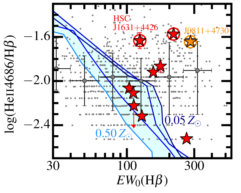
Figure 7.— Same as Figure 6, but as a function of H$\beta$ equivalent width, $\textrm{EW}_{0}$(H$\beta$). Symbols are the same as in Figures 5 and 6. Here we do not show HSC J2314$+$0154, whose $T_{\mathrm{e}}$-metallicity and element abundances are not estimated. Solid lines represent the S19 HMXB models, tracing time evolution of He ii4686/H$\beta$ and $\textrm{EW}_{0}$(H$\beta$) with different metallicities of 0.05, 0.10, 0.20, and 0.50 $Z_{\odot}$ (from dark blue to light blue).

Figure 7 compares He ii4686/H$\beta$ ratios of our metal-poor galaxies and those obtained by the S19 HMXB models (solid lines) as a function of $\textrm{EW}_{0}$(H$\beta$). The solid lines trace time evolution of He ii4686/H$\beta$ and $\textrm{EW}_{0}$(H$\beta$) with different metallicities of 0.05, 0.10, 0.20, and 0.50 $Z_{\odot}$. The $\textrm{EW}_{0}$(H$\beta$) decreases and the He ii4686/H$\beta$ ratio increases as time passes due to the stellar evolution and HMXB evolution, respectively. The HMXB models (especially 0.05 and 0.10$Z_{\odot}$) show a rapid increase of He ii4686/H$\beta$ around $\textrm{EW}_{0}$(H$\beta$)$\sim$100–300 Å. The $\textrm{EW}_{0}$(H$\beta$)$\sim$100–300 Å corresponds to $\sim$5 Myr in the bpass binary stellar synthesis models. The rapid increase is triggered by the first compact object formation (i.e., the first HMXB formation) after $\sim$5 Myr of the starburst. As shown in Figure 7, the HMXB models of S19 have quantitatively explained the He ii4686/H$\beta$ ratios of half of our metal-poor galaxies. However, we find that the other five metal-poor galaxies are not explained by the HMXB model, which fall in the ranges of $\textrm{EW}_{0}$(H$\beta$)$>$100 Å and $\log$(He ii4686/H$\beta$)$>$$-2.0$. Interestingly, three out of the five metal-poor galaxies are EMPGs (i.e., $Z<0.1Z_{\odot}$), which are marked with red and orange circles in Figure 7. Especially, HSC J1631$+$4426 ($0.016Z_{\odot}$) and J0811$+$4730 ($0.019Z_{\odot}$) are the representative EMPGs with the two lowest metallicities reported to date, showing high He ii4686/H$\beta$ ratios of $\log$(He ii4686/H$\beta$)$\sim$$-1.6$. Furthermore, the S19 SFG sample also include galaxies in the same ranges of $\textrm{EW}_{0}$(H$\beta$)$>$100 Å and $\log$(He ii4686/H$\beta$)$>$$-2.0$. S19 have argued that other X-ray sources are likely to appear fairly soon after the onset of the star formation ($\lesssim$5 Myr) in galaxies with high values of $\textrm{EW}_{0}$(H$\beta$) and He ii4686/H$\beta$. Although WR stars might contribute to the strong He ii4686 emission, we do not find broad He ii4686 emission lines typical of the WR stars (Brinchmann et al., 2008; López-Sánchez & Esteban, 2009) in our spectra. Instead, S19 suggest that an underlying older population or shocks could also contribute to the high He ii4686/H$\beta$ ratios. S19 do not discuss the metallicity in the explanation of the large He ii4686/H$\beta$ ratios at $\textrm{EW}_{0}$(H$\beta$)$>$100 Å. However, the two EMPGs (HSC J1631$+$4426 and J0811$+$4730) in this paper emphasize that both the $\textrm{EW}_{0}$(H$\beta$) and metallicity may be keys to explain the He ii4686/H$\beta$ ratios higher than the HMXB models.

In addition to the S19 suggestions, we propose two other possibilities, for the first time, which can explain the high He ii4686/H$\beta$ ratios seen in the range of $\textrm{EW}_{0}$(H$\beta$)$>$100 Å. First, we propose a possibility of super massive stars beyond 300 $M_{\odot}$. The HMXB models of Fragos et al. (2013a, b) assume the Kroupa IMF (Kroupa, 2001; Kroupa & Weidner, 2003) with the maximum stellar mass of $M_{\mathrm{max}}$$=$120 $M_{\odot}$. Thus, in the HMXB models of (Fragos et al., 2013a, b), the first HMXBs emerge $\sim$ 5 Myr after the start of the star formation, which corresponds to a lifetime of a star with 120 $M_{\odot}$. On the other hand, stars more massive than 120 $M_{\odot}$ are expected to have a shorter life time than stars with 120 $M_{\odot}$. According to the theoretical study of Yungelson et al. (2008), super massive stars with 300 $M_{\odot}$ and 1000 $M_{\odot}$ die after 2.5 and 2.0 Myr after the onset of the star formation, respectively. As described in Section 5.1.3, stars between 140 and 300 $M_{\odot}$ undergo thermonuclear explosions triggered by PISNe (Barkat et al., 1967), and do not leave any compact object (e.g., Heger & Woosley, 2002). On the other hand, stars beyond 300 $M_{\odot}$ experience core-collapse SNe and form IMBHs (e.g., Ohkubo et al., 2006). Ohkubo et al. (2006) estimate that BH masses become $\sim$230 and $\sim$500 $M_{\odot}$ for stars with initial masses of 500 and 1000 $M_{\odot}$, respectively. Thus, when we assume super massive stars beyond 300 $M_{\odot}$, IMBHs appear as early as $\sim$2 Myr, and part of the IMBHs may form HMXBs. Accretion disks of IMBHs emit very hard radiation including ionizing photons above 54.4 eV, which boosts the He ii4686 intensity. A galaxy as young as $\sim$2 Myr has $\textrm{EW}_{0}$(H$\beta$)$\sim$300–400Å according to the bpass models. Under the assumption of super massive stars beyond 300 $M_{\odot}$, the He ii4686/H$\beta$ ratio is expected to start increasing at around $\textrm{EW}_{0}$(H$\beta$)$\sim$300–400Å. Such a model may cover the regions of $\textrm{EW}_{0}$(H$\beta$)$>$100 Å and $\log$(He ii4686/H$\beta$)$>$$-2.0$ shown in Figure 7. Thus, we suggest that super massive stars beyond 300 $M_{\odot}$ would be able to explain the high ratios, $\log$(He ii4686/H$\beta$)$>$$-2.0$ in the galaxies with $\textrm{EW}_{0}$(H$\beta$)$>$100 Å. Note again that galaxies with $\log$(He ii4686/H$\beta$)$>$$-2.0$ and $\textrm{EW}_{0}$(H$\beta$)$>$100 Å includes EMPGs, HSC J1631$+$4426 SDSS J2115$-$1734, and J0811$+$4730. These EMPGs might form super massive star beyond 300 $M_{\odot}$ from their extremely metal-poor gas. However, our explanation and the interpretation of S19 are based on some simple assumptions that associate the HMXB models and the bpass stellar synthesis models. We propose to construct self-consistent SED models ranging from X-ray to UV with the HMXB evolution models under the assumption of $M_{\mathrm{max}}$$>$300 $M_{\odot}$.

Second, we also suggest a possibility of a metal-poor AGN, which can contribute to boost the He ii4686 intensity of the very young galaxies. In Paper I, we have confirmed that all of our metal-poor galaxies fall on the SFG region of the BPT diagram defined by the maximum photoionization models with stellar radiation (Kewley et al., 2001). However, Kewley et al. (2013) suggest that emission-line ratios calculated under the assumption of a metal-poor AGN also fall on the SFG region. Thus, we cannot exclude the possibility of a metal-poor AGN. Groves et al. (2004a, b) have constructed the photo-ionization models under the assumption of AGN-like, power-row radiation. The models of Groves et al. (2004a, b) predict very strong He ii4686 emission represented by $\log$(He ii4686/H$\beta$)$\sim$$-1.5$ to 0.0. On the other hand, photo-ionization models with stellar radiation (Xiao et al., 2018) predict $\log$(He ii4686/H$\beta$)$\lesssim$$-2.5$. To explain the observed ratios of $\log$(He ii4686/H$\beta$)$\sim$$-2.0$, the combination of AGN and stellar radiation is required. We have checked the archival data of ROSAT and XMM, and found no detection in X-ray. This is because the data are $\sim$2 orders of magnitudes shallower than expected X-ray luminosities ($\sim$10^-14 erg s^-1 cm^-2) of our metal-poor galaxy sample, which are obtained under the assumption of $L_{\mathrm{2keV}}$–$M_{\mathrm{UV}}$ relation of AGN (Lusso et al., 2010). Deep X-ray observations are required to constrain X-ray sources of metal-poor galaxies.

5.3. Formation Mechanism of Super Massive Stars beyond 300 $M_{\odot}$

Below, we focus only on the two representative EMPGs, HSC J1631$+$4426 (0.016 $Z_{\odot}$) and J0811$+$4730 (0.019 $Z_{\odot}$) and discuss their high Fe/O ratios and He ii4686/H$\beta$ ratios. The two representative EMPGs, HSC J1631$+$4426 and J0811$+$4730 show the two lowest metallicities reported to date. In Section 5.1.3, we have found that the two EMPGs, HSC J1631$+$4426 and J0811$+$4730 show Fe/O ratios $\sim$1.0 dex higher than Galactic stars and the Fe/O evolution models at fixed metallicity. We have concluded that the high Fe/O ratios are explained by core-collapse SNe of super massive stars beyond 300 $M_{\odot}$. In Section 5.2.2, we have also found that the two EMPGs, HSC J1631$+$4426 and J0811$+$4730, show both high He ii4686/H$\beta$ ratios ($\sim$1/40) and high $\textrm{EW}_{0}$(H$\beta$) ($\sim$100–300 Å). We have suggested that IMBH formed from super massive stars beyond 300 $M_{\odot}$ can explain the high He ii4686/H$\beta$ ratios. Interestingly, the scenario of super massive stars beyond 300 $M_{\odot}$ explains both the high Fe/O ratios and the high He ii4686/H$\beta$ ratios of our EMPGs with the low metallicities ($\sim$0.02 $Z_{\odot}$), young ages ($\lesssim$50 Myr), and very low stellar mass ($\sim$10⁵–10⁶ $M_{\odot}$), which are undergoing early phases of the galaxy formation. We propose, for the first time, the connection between the large He ii4686/H$\beta$ ratios (Section 5.2.2) and the solar Fe/O ratios (Section 5.1.3).

The idea of super massive stars beyond 300 $M_{\odot}$ is not necessarily extraordinary. Crowther et al. (2010, 2016) have claimed the spectroscopic identification of super massive stars with $\sim$320 $M_{\odot}$ in the R136 star cluster of LMC. The identification of an IMBH with $M_{\mathrm{BH}}>700M_{\odot}$ in a star cluster of M82 (Matsumoto et al., 2001; Ebisuzaki et al., 2001; Kaaret et al., 2001) is another indirect trace of a super massive star beyond 300 $M_{\odot}$. This is because the SN numerical simulation (Ohkubo et al., 2006) suggests that a star with initial masses beyond 300 $M_{\odot}$ leaves an IMBH with $\gtrsim$100 $M_{\odot}$.

We may wonder how such super massive stars are formed. Below, we discuss the formation mechanisms of super massive stars beyond 300 $M_{\odot}$. Theoretical studies (e.g., Bromm & Loeb, 2004; Omukai & Palla, 2003) suggest that metal-free (pop-III) stars are typically super massive ($>$300 $M_{\odot}$) because gas cooling becomes insufficient and the fragmentation mass becomes large in metal-free gas. The critical metallicity ($Z_{\mathrm{crit}}$), below which super massive stars can be formed directly, is $Z_{\mathrm{crit}}\sim 10^{-6}$ to $10^{-4}$$Z_{\odot}$, theoretically (e.g., Bromm et al., 2001; Santoro & Shull, 2006; Schneider et al., 2006; Smith & Sigurdsson, 2007). The critical metallicity ($Z_{\mathrm{crit}}\sim 10^{-6}$–$10^{-4}$$Z_{\odot}$) is much lower than our metallicity measurements of our EMPGs, $\sim$0.02 $Z_{\odot}$. Thus, the direct gas collapse is unlikely to be the formation mechanism of the super massive stars beyond 300 $M_{\odot}$ in our EMPGs.

We briefly discuss another possibility that EMPGs previously had a metallicity near the critical metallicity ($\sim 10^{-6}$–$10^{-4}$$Z_{\odot}$) at the time of the galaxy formation, and the metallicity has been increased by SNe within a short period. The metallicity at the time of the galaxy formation namely depends on the metallicity of the inflow gas, which may come from a void region free from the metal contamination. Based on the observational results of metal-poor galaxies, Thuan et al. (2005) speculate that the metallicity lower limit (so-called “metallicity floor”) might exist at $\sim 10^{-2}$$Z_{\odot}$ at $z=0$ because the IGM has slightly been metal-enriched by the past star formation activities even in the void regions. In addition, observational studies of Lyman alpha absorption systems (e.g., Prochaska et al., 2003; Rafelski et al., 2012; Lehner et al., 2013; Quiret et al., 2016) have not yet discovered Lyman alpha absorption system below $\sim 10^{-2}$$Z_{\odot}$ at $z=0$–$1$. Hydrodynamical simulation of Martizzi et al. (2019) also demonstrates that the average IGM metallicity in the void region is $\sim 10^{-2}$$Z_{\odot}$ at $z=0$. We do not necessarily remove the possibility that EMPGs had a metallicity near the critical metallicity ($\sim 10^{-6}$–$10^{-4}$$Z_{\odot}$) at the time of the galaxy formation because part of the IGM would reach below $\sim 10^{-2}$$Z_{\odot}$ (Hafen et al., 2017) due to a metallicity fluctuation. However, the direct gas collapse may not be, at least, the main formation mechanism of the super massive stars beyond 300 $M_{\odot}$.

Ebisuzaki et al. (2001) and Portegies Zwart et al. (1999, 2004, 2006) has presented another formation mechanism of super massive stars beyond 300 $M_{\odot}$, where super massive stars are formed by stellar mergers under the very dense condition in a star cluster. Numerical simulations suggest that super massive stars of 800–3000 $M_{\odot}$ have been formed by stellar mergers within $\sim$3 Myr (Portegies Zwart et al., 2004). The super massive star formation mechanism of Portegies Zwart et al. (2004) is presented to explain an IMBH discovered in a star cluster of M82 (Matsumoto et al., 2001; Ebisuzaki et al., 2001; Kaaret et al., 2001). The estimated BH mass of the M82 IMBH is $M_{\mathrm{BH}}>700M_{\odot}$. This stellar merger mechanism requires the very dense star forming regions, which are typical in young, metal-poor galaxies. Indeed, our sample EMPGs are undergoing the intensive star-formation represented by high sSFRs ($\sim$300 Gyr^-1, Kojima et al., 2020) and small sizes ($\sim$ 100 pc, Paper III). Although the stellar merger mechanism itself does not depend on metallicity, the formation mechanism of the very dense star forming regions may depend on metallicity. A possible scenario is that a large amount of massive stars are formed within a compact region by a primordial gas (i.e., almost metal free) infall from the inter-galactic space (KS1-EMPG in Paper III). This scenario may be associated with the top heavy IMF.

In this paper, we find that two representative EMPGs ($\sim$0.02 $Z_{\odot}$) show both the high Fe/O ratios and the high He ii4686/H$\beta$ ratios, which are not explained by the previous models assuming massive stars up to $100$ or $120$ $M_{\odot}$. In the end of this section, we summarize one possible picture that we have suggested in each section of this paper. In our picture, EMPGs are formed by a primordial gas infall, which also forms star clusters with a very high number density of massive stars (Paper III). In such very dense regions of star clusters, stellar mergers trigger the formation of super massive stars beyond 300 $M_{\odot}$ within $\sim$3 Myr (Portegies Zwart et al., 2004). The super massive stars beyond 300 $M_{\odot}$ eventually eject much iron through the core-collapse SNe in $\sim$2 Myr (Ohkubo et al., 2006; Yungelson et al., 2008) and form IMBHs ($M_{\mathrm{BH}}\gtrsim 100M_{\odot}$, Ohkubo et al., 2006) boosting the He ii4686 emission. To testify this picture, spectroscopic observations are required with a high spacial resolution in multi-wavelength to identify the formation mechanism of EMPGs and to directly detect IMBH signatures in EMPGs.

6. SUMMARY

We investigate element abundance ratios and ionizing radiation of 10 metal-poor galaxies at $z\lesssim 0.03$, which have been discovered in the wide-field imaging data of Subaru/Hyper Sprime-Cam (HSC) and Sloan Digital Sky Survey (SDSS) by Kojima et al. (2020). The 10 metal-poor galaxies are represented by low metallicities, $12$+$\log({\rm O/H})$ =6.90–8.45, low stellar masses, $\log$($M_{\star}$/$M_{\odot}$)$=$4.95–7.06, and high specific star-formation rates (sSFR$\sim$300 Gyr^-1). These galaxies have very low masses of $\log$($M_{\star}$/$M_{\odot}$)$\lesssim$6, which are comparable to those of star clusters. Such cluster-like galaxies are undergoing very early phases of the galaxy formation. Especially, three out of the 10 galaxies are extremely metal-poor galaxies (EMPGs) defined by $12$+$\log({\rm O/H})$$<$7.69, including HSC J1631$+$4426 with the lowest metallicity (0.016 $Z_{\odot}$) reported to date. In addition to the 10 metal-poor galaxies, we include another EMPG from the literature (J0811$+$4730, Izotov et al., 2018) in the sample of this paper. J0811$+$4730 has the second lowest metallicity of 0.019 $Z_{\odot}$ reported to date. The two EMPGs (HSC J1631$+$4426 and J0811$+$4730) are key in this paper.

• We estimate element abundance ratios of Ne/O, Ar/O, and N/O of our metal-poor galaxies, and compare them with local SFGs. We find that $\alpha$-element ratios of Ne/O and Ar/O show almost constant values of $\log$(Ne/O) $\sim$$-0.8$ and $\log$(Ar/O)$\sim$$-2.5$ as a function of metallicity, respectively. These constant Ne/O and Ar/O values are consistent with those of local SFGs. Most of our metal-poor galaxies have N/O ratios of $\log$(N/O)$\lesssim$$-1.5$, suggesting that our metal-poor galaxies are undergoing the primary nucleosynthesis of nitrogen due to their low metallicity and young stellar population.

• We also estimate Fe/O ratios of our metal-poor galaxies, and compare them with local SFGs. Our metal-poor galaxy sample shows a decreasing Fe/O trend with increasing metallicity, which is consistent with the previous results of local SFGs. We find that two EMPGs, HSC J1631$+$4426 (0.016 $Z_{\odot}$) and J0811$+$4730 (0.019 $Z_{\odot}$, Izotov et al., 2018), show higher Fe/O ratios than observational results of Galactic stars and a model calculation of the Fe/O evolution at fixed metallicity. Especially, HSC J1631$+$4426 and J0811$+$4730 show the solar Fe/O ratios in spite of its very low metallicity, 0.016 and 0.019 $Z_{\odot}$, respectively. We discuss the three scenarios that might be able to explain the high Fe/O ratios with the extremely low metallicity: (1) the preferential dust depletion of iron, (2) a combination of metal enrichment and gas dilution caused by inflow, and (3) super massive stars beyond 300 $M_{\odot}$. The scenario (1) is ruled out because the solar Fe/O ratios are not achieved by the dust depletion, and we do not see any correlation between the dust extinction and the Fe/O ratios. We also exclude the scenario (2) because the observed N/O ratios are lower than the expected solar N/O ratio when the scenario (2) is true. Thus, we conclude that the high Fe/O ratios of the two EMPGs are attributed to super massive stars beyond 300 $M_{\odot}$, which is consistent with the young stellar ages of EMPGs ($\lesssim 50$ Myr).

• To probe ionizing radiation in our metal-poor galaxies, we inspect emission lines from various ions covering a wide range of ionization potentials. We choose H$\beta$, [O ii]3727,3729, [Ar iii]4740, [O iii]5007, and [Ar iv]7136 lines, which are sensitive to ionizing photon above 13.6, 13.6, 27.6, 35.1, and 40.7 eV, respectively. Our metal-poor galaxies and local, average SFGs show sequences of [O ii]3727,3729/H$\beta$, [Ar iii]4740/H$\beta$, [O iii]5007/H$\beta$, and [Ar iv]7136/H$\beta$ as a function of metallicity, and match each other within small scatters. The match between the two samples suggests that our metal-poor galaxies and local, average SFGs have a similar spectral shape in the energy range of 13.6–40.7 eV for a given metallicity.

• We find that five metal-poor galaxies show both high He ii4686/H$\beta$ ratios ($>$1/100) and high $\textrm{EW}_{0}$(H$\beta$) ($>$100 Å). Interestingly, two out of the five metal-poor galaxies are the representative EMPGs, HSC J1631$+$4426 (0.016 $Z_{\odot}$) and J0811$+$4730 (0.019 $Z_{\odot}$). These high He ii4686/H$\beta$ ratios and high $\textrm{EW}_{0}$(H$\beta$) are not explained by the latest binary population stellar synthesis model and the latest HMXB model, where a maximum stellar mass cut, 120 $M_{\odot}$ is used. We suggest that super massive stars beyond 300 $M_{\odot}$ can explain the high He ii4686/H$\beta$ ratios for galaxies of $\textrm{EW}_{0}$(H$\beta$)$>$100 Å (i.e., $\lesssim$5 Myr). Super massive stars beyond 300 $M_{\odot}$ have very short lifetimes of $\sim$2 Myr, and form intermediate-mass black holes (IMBHs) of $\gtrsim$100 $M_{\odot}$ as early as $\sim$2 Myr after the onset of the star formation. We do not rule out a possibility of a metal-poor AGN, which can contribute to the He ii4686 boost of the very young galaxies even at $\lesssim$5 Myr.

• Interestingly, the scenario of super massive stars beyond 300 $M_{\odot}$ explains both the high Fe/O ratios and the high He ii4686/H$\beta$ ratios of our EMPGs. We also discuss a formation mechanism of super massive stars beyond 300 $M_{\odot}$. The direct collapse of metal-poor gas is unlikely to be the formation mechanism because the critical metallicity ($Z_{\mathrm{crit}}\sim 10^{-6}$–$10^{-4}$$Z_{\odot}$), below which super massive stars can be formed directly, is much lower than the metallicities of the two representative EMPGs, $\sim$0.02 $Z_{\odot}$. Instead, super massive stars beyond 300 $M_{\odot}$ would be formed by stellar mergers under the very dense condition in a star cluster. In this picture, EMPGs are formed by a primordial gas infall, which also forms star clusters with a very high number density of massive stars. In such very dense regions, stellar mergers trigger the formation of super massive stars beyond 300 $M_{\odot}$ within $\sim$3 Myr. The super massive stars beyond 300 $M_{\odot}$ eventually eject much iron through the core-collapse SNe in $\sim$2 Myr and form IMBHs ($M_{\mathrm{BH}}\gtrsim 100M_{\odot}$) boosting the He ii4686 emission.

References

- Aihara et al. (2018) Aihara, H., Arimoto, N., Armstrong, R., et al. 2018, PASJ, 70, 1
- Aihara et al. (2019) Aihara, H., AlSayyad, Y., Ando, M., et al. 2019, PASJ, 71, 114
- Albareti et al. (2017) Albareti, F. D., Prieto, C. A., Almeida, A., et al. 2017, ApJS, 233, 25
- Allen et al. (2008) Allen, M. G., Groves, B. A., Dopita, M. A., Sutherland, R. S., & Kewley, L. J. 2008, ApJS, 178, 20
- Andrews & Martini (2013) Andrews, B. H., & Martini, P. 2013, ApJ, 765, 140
- Asplund et al. (2009) Asplund, M., Grevesse, N., Sauval, A. J., & Scott, P. 2009, ARA&A, 47, 481
- Axelrod et al. (2010) Axelrod, T., Kantor, J., Lupton, R. H., & Pierfederici, F. 2010, in Proc. SPIE, ed. N. M. Radziwill & A. Bridger, Vol. 7740, 774015
- Baldwin et al. (1981) Baldwin, A., Phillips, M. M., & Terlevich, R. 1981, PASP, 93, 817
- Barkat et al. (1967) Barkat, Z., Rakavy, G., & Sack, N. 1967, PRL, 18, 379
- Bensby & Feltzing (2006) Bensby, T., & Feltzing, S. 2006, MNRAS, 367, 1181
- Bensby et al. (2013) Bensby, T., Yee, J. C., Feltzing, S., et al. 2013, A&A, 549, A147
- Bosch et al. (2018) Bosch, J., Armstrong, R., Bickerton, S., et al. 2018, PASJ, 70, 1
- Brinchmann et al. (2008) Brinchmann, J., Kunth, D., & Durret, F. 2008, A&A, 485, 657
- Bromm et al. (2001) Bromm, V., Ferrara, A., Coppi, P., & Larson, R. 2001, MNRAS, 328, 969
- Bromm & Loeb (2004) Bromm, V., & Loeb, A. 2004, New Astronomy, 9, 353
- Campbell et al. (1986) Campbell, A., Terlevich, R., & Melnick, J. 1986, MNRAS, 223, 811
- Cardelli et al. (1989) Cardelli, J. A., Clayton, G. C., & Mathis, J. S. 1989, ApJ, 345, 245
- Cayrel et al. (2004) Cayrel, R., Depagne, E., Spite, M., et al. 2004, A&A, 416, 1117
- Christensen et al. (2012a) Christensen, L., Laursen, P., Richard, J., et al. 2012a, MNRAS, 427, 1973
- Christensen et al. (2012b) Christensen, L., Richard, J., Hjorth, J., et al. 2012b, MNRAS, 427, 1953
- Coupon et al. (2018) Coupon, J., Czakon, N., Bosch, J., et al. 2018, PASJ, 70, 1
- Crowther & Hadfield (2006) Crowther, P. A., & Hadfield, L. J. 2006, A&A, 449, 711
- Crowther et al. (2010) Crowther, P. A., Schnurr, O., Hirschi, R., et al. 2010, MNRAS, 408, 731
- Crowther et al. (2016) Crowther, P. A., Caballero-Nieves, S. M., Bostroem, K. A., et al. 2016, MNRAS, 458, 624
- Ebisuzaki et al. (2001) Ebisuzaki, T., Makino, J., Tsuru, T. G., et al. 2001, ApJ, 562, L19
- Eldridge et al. (2017) Eldridge, J. J., Stanway, E. R., Xiao, L., et al. 2017, PASA, 34, e058
- Elmegreen & Elmegreen (2017) Elmegreen, D. M., & Elmegreen, B. G. 2017, ApJ, 851, L44
- Ferland et al. (2013) Ferland, G. J., Porter, R. L., Van Hoof, P. A. M., et al. 2013, RMxAA, 49, 137
- Fischer & Tachiev (2004) Fischer, C. F., & Tachiev, G. 2004, Atomic Data and Nuclear Data Tables, 87, doi:10.1016/j.adt.2004.02.001
- Fragos et al. (2013a) Fragos, T., Lehmer, B. D., Naoz, S., Zezas, A., & Basu-Zych, A. 2013a, ApJL, 776, L31
- Fragos et al. (2013b) Fragos, T., Lehmer, B., Tremmel, M., et al. 2013b, ApJ, 764, 41
- Furusawa et al. (2018) Furusawa, H., Koike, M., Takata, T., et al. 2018, PASJ, 70, 1
- Galavís et al. (1997) Galavís, M. E., Mendoza, C., & Zeippen, C. J. 1997, A&AS, 123, 159
- Garnett (1992) Garnett, D. R. 1992, AJ, 103, 1330
- Gratton et al. (2003) Gratton, R. G., Carretta, E., Claudi, R., Lucatello, S., & Barbieri, M. 2003, A&A, 404, 187
- Groves et al. (2004a) Groves, B. A., Dopita, M. A., & Sutherland, R. S. 2004a, ApJS, 153, 9
- Groves et al. (2004b) —. 2004b, ApJS, 153, 75
- Guseva et al. (2017) Guseva, N. G., Izotov, Y. I., Fricke, K. J., & Henkel, C. 2017, A&A, 599, A65
- Hafen et al. (2017) Hafen, Z., Faucher-Giguère, C.-A., Anglés-Alcázar, D., et al. 2017, MNRAS, 469, 2292
- Hanuschik (2003) Hanuschik, R. W. 2003, A&A, 407, 1157
- Harikane et al. (2018) Harikane, Y., Ouchi, M., Shibuya, T., et al. 2018, ApJ, 859, 84
- Heger & Woosley (2002) Heger, A., & Woosley, S. E. 2002, ApJ, 567, 532
- Isobe et al. (2020) Isobe, Y., Ouchi, M., Kojima, T., et al. 2020, arXiv e-prints, arXiv:2004.11444
- Ivezić et al. (2019a) Ivezić, Ž., Kahn, S. M., Tyson, J. A., et al. 2019a, ApJ, 873, 111
- Ivezić et al. (2019b) —. 2019b, ApJ, 873, 111
- Iwamoto et al. (1999) Iwamoto, K., Brachwitz, F., Nomoto, K., et al. 1999, ApJS, 125, 439
- Izotov et al. (2009) Izotov, Y. I., Guseva, N. G., Fricke, K. J., & Papaderos, P. 2009, A&A, 503, 61
- Izotov et al. (2006a) Izotov, Y. I., Schaerer, D., Blecha, A., et al. 2006a, A&A, 459, 71
- Izotov et al. (2006b) Izotov, Y. I., Stasińska, G., Meynet, G., Guseva, N. G., & Thuan, T. X. 2006b, A&A, 448, 955
- Izotov & Thuan (1998) Izotov, Y. I., & Thuan, T. X. 1998, ApJ, 497, 227
- Izotov & Thuan (1999) —. 1999, ApJ, 511, 639
- Izotov et al. (2012) Izotov, Y. I., Thuan, T. X., & Guseva, N. G. 2012, A&A, 546, A122
- Izotov et al. (2019) —. 2019, MNRAS, 483, 5491
- Izotov et al. (2018) Izotov, Y. I., Thuan, T. X., Guseva, N. G., & Liss, S. E. 2018, MNRAS, 473, 1956
- Johansson et al. (2000) Johansson, S., Zethson, T., Hartman, H., et al. 2000, A&A, 361, 977
- Jurić et al. (2015) Jurić, M., Kantor, J., Lim, K.-T., et al. 2015, arXiv e-prints, arXiv:1512.07914
- Kaaret et al. (2001) Kaaret, P., Prestwich, A. H., Zezas, A., et al. 2001, MNRAS, 321, L29
- Kawanomoto et al. (2018) Kawanomoto, S., Uraguchi, F., Komiyama, Y., et al. 2018, PASJ, 70, 1
- Kelson (2003) Kelson, D. 2003, PASP, 115, 688
- Kelson et al. (2000) Kelson, D. D., Illingworth, G. D., van Dokkum, P. G., & Franx, M. 2000, ApJ, 531, 159
- Kennicutt (1998) Kennicutt, R. C. 1998, ARA&A, 36, 189
- Kewley et al. (2013) Kewley, L. J., Dopita, M. A., Leitherer, C., et al. 2013, ApJ, 774, 100
- Kewley et al. (2001) Kewley, L. J., Dopita, M. A., Sutherland, R. S., Heisler, C. A., & Trevena, J. 2001, ApJ, 556, 121
- Kisielius et al. (2009) Kisielius, R., Storey, P. J., Ferland, G. J., & Keenan, F. P. 2009, MNRAS, 397, 903
- Kojima et al. (2017) Kojima, T., Ouchi, M., Nakajima, K., et al. 2017, PASJ, 69, 1
- Kojima et al. (2020) Kojima, T., Ouchi, M., Rauch, M., et al. 2020, ApJ, 898, 142
- Komiyama et al. (2018) Komiyama, Y., Obuchi, Y., Nakaya, H., et al. 2018, PASJ, 70, 1
- Kroupa (2001) Kroupa, P. 2001, MNRAS, 322, 231
- Kroupa & Weidner (2003) Kroupa, P., & Weidner, C. 2003, ApJ, 598, 1076
- Kunth & Östlin (2000) Kunth, D., & Östlin, G. 2000, A&A, 10, 1
- Lecureur et al. (2007) Lecureur, A., Hill, V., Zoccali, M., et al. 2007, A&A, 465, 799
- Legrand et al. (1997) Legrand, F., Kunth, D., Roy, J. R., Mas-Hesse, J. M., & Walsh, J. R. 1997, A&A, 326, 18
- Lehner et al. (2013) Lehner, N., Howk, J. C., Tripp, T. M., et al. 2013, ApJ, 770, doi:10.1088/0004-637X/770/2/138
- López-Sánchez & Esteban (2009) López-Sánchez, A. R., & Esteban, C. 2009, A&A, 508, 615
- López-Sánchez & Esteban (2010) López-Sánchez, Á. R., & Esteban, C. 2010, A&A, 516, A104
- Luridiana et al. (2015) Luridiana, V., Morisset, C., & Shaw, R. A. 2015, A&A, 573, A42
- Lusso et al. (2010) Lusso, E., Comastri, A., Vignali, C., et al. 2010, A&A, 512, A34
- Ly et al. (2014) Ly, C., Malkan, M. A., Nagao, T., et al. 2014, ApJ, 780, 122
- Mainali et al. (2017) Mainali, R., Kollmeier, J. A., Stark, D. P., et al. 2017, ApJ, 836, L14
- Martizzi et al. (2019) Martizzi, D., Vogelsberger, M., Artale, M. C., et al. 2019, MNRAS, 486, 3766
- Matsumoto et al. (2001) Matsumoto, H., Tsuru, T. G., Koyama, K., et al. 2001, ApJ, 547, L25
- McLaughlin & Bell (2000) McLaughlin, B. M., & Bell, K. L. 2000, Journal of Physics B: Atomic, Molecular and Optical Physics, 33, 597
- Mendoza & Zeippen (1982) Mendoza, C., & Zeippen, C. J. 1982, MNRAS, 198, 127
- Miyazaki et al. (2012) Miyazaki, S., Komiyama, Y., Nakaya, H., et al. 2012, in Proc. SPIE, ed. I. S. McLean, S. K. Ramsay, & H. Takami, 84460Z
- Miyazaki et al. (2018) Miyazaki, S., Komiyama, Y., Kawanomoto, S., et al. 2018, PASJ, 70, 1
- Munoz Burgos et al. (2009) Munoz Burgos, J. M., Loch, S. D., Ballance, C. P., & Boivin, R. F. 2009, A&A, 500, 1253
- Nakajima et al. (2016) Nakajima, K., Ellis, R. S., Iwata, I., et al. 2016, ApJ, 831, L9
- Nakajima & Ouchi (2014) Nakajima, K., & Ouchi, M. 2014, MNRAS, 442, 900
- Nomoto et al. (2013) Nomoto, K., Kobayashi, C., & Tominaga, N. 2013, ARA&A, 51, 457
- Nugis & Lamers (2000) Nugis, T., & Lamers, H. J. 2000, A&A, 360, 227
- Ohkubo et al. (2006) Ohkubo, T., Umeda, H., Maeda, K., et al. 2006, ApJ, 645, 1352
- Oke & Gunn (1983) Oke, J. B., & Gunn, J. E. 1983, ApJ, 266, 713
- Omukai & Palla (2003) Omukai, K., & Palla, F. 2003, ApJ, 589, 677
- Ono et al. (2010) Ono, Y., Ouchi, M., Shimasaku, K., et al. 2010, ApJ, 724, 1524
- Ono et al. (2018) Ono, Y., Ouchi, M., Harikane, Y., et al. 2018, PASJ, 70, 2
- Pérez-Montero & Contini (2009) Pérez-Montero, E., & Contini, T. 2009, MNRAS, 398, 949
- Pérez-Montero et al. (2013) Pérez-Montero, E., Contini, T., Lamareille, F., et al. 2013, A&A, 549, A25
- Portegies Zwart et al. (2004) Portegies Zwart, S. F., Baumgardt, H., Hut, P., Makino, J., & McMillan, S. L. 2004, Nature, 428, 724
- Portegies Zwart et al. (2006) Portegies Zwart, S. F., Baumgardt, H., McMillan, S. L. W., et al. 2006, ApJ, 641, 319
- Portegies Zwart et al. (1999) Portegies Zwart, S. F., Makino, J., McMillan, S. L., & Hut, P. 1999, A&A, 348, 117
- Press et al. (2007) Press, W. H., Teukolsky, S. A., Vetterling, T. W., & Flannery, B. P. 2007, Numerical Recipies, The Art of Scientific Computing (Cambridge University Press)
- Prochaska et al. (2003) Prochaska, J. X., Gawiser, E., Wolfe, A. M., Castro, S., & Djorgovski, S. G. 2003, ApJ, 595, L9
- Quinet (1996) Quinet, P. 1996, A&AS, 116, 573
- Quiret et al. (2016) Quiret, S., Péroux, C., Zafar, T., et al. 2016, MNRAS, 458, 4074
- Rafelski et al. (2012) Rafelski, M., Wolfe, A. M., Prochaska, J. X., Neeleman, M., & Mendez, A. J. 2012, ApJ, 755, 89
- Ramsbottom & Bell (1997) Ramsbottom, C., & Bell, K. 1997, Atomic Data and Nuclear Data Tables, 66, 65
- Rodriguez (2003) Rodriguez, M. 2003, ApJ, 590, 296
- Rodriguez & Rubin (2005) Rodriguez, M., & Rubin, R. H. 2005, ApJ, 626, 900
- Santoro & Shull (2006) Santoro, F., & Shull, J. M. 2006, ApJ, 643, 26
- Saxena et al. (2020a) Saxena, A., Pentericci, L., Mirabelli, M., et al. 2020a, A&A, 636, arXiv:1911.09999
- Saxena et al. (2020b) Saxena, A., Pentericci, L., Schaerer, D., et al. 2020b, MNRAS, 496, 3796
- Schaerer et al. (2019) Schaerer, D., Fragos, T., & Izotov, Y. I. 2019, A&A, 622, L10
- Schlegel et al. (1998) Schlegel, D. J., Finkbeiner, D. P., & Davis, M. 1998, ApJ, 500, 525
- Schneider et al. (2006) Schneider, R., Omukai, K., Inoue, A. K., & Ferrara, A. 2006, MNRAS, 369, 1437
- Senchyna et al. (2019) Senchyna, P., Stark, D. P., Chevallard, J., et al. 2019, MNRAS, 488, 3492
- Senchyna et al. (2020) Senchyna, P., Stark, D. P., Mirocha, J., et al. 2020, MNRAS, 494, 941
- Senchyna et al. (2017) Senchyna, P., Stark, D. P., Vidal-García, A., et al. 2017, MNRAS, 472, 2608
- Shapley et al. (2017) Shapley, A. E., Sanders, R. L., Reddy, N. A., et al. 2017, ApJ, 846, L30
- Shirazi & Brinchmann (2012) Shirazi, M., & Brinchmann, J. 2012, MNRAS, 421, 1043
- Skillman (1989) Skillman, E. D. 1989, ApJ, 347, 883
- Smith & Sigurdsson (2007) Smith, B. D., & Sigurdsson, S. 2007, ApJ, 661, L5
- Stanway et al. (2016) Stanway, E. R., Eldridge, J. J., & Becker, G. D. 2016, MNRAS, 456, 485
- Stark et al. (2014) Stark, D. P., Richard, J., Siana, B., et al. 2014, MNRAS, 445, 3200
- Stark et al. (2015) Stark, D. P., Walth, G., Charlot, S., et al. 2015, MNRAS, 454, 1393
- Stark et al. (2017) Stark, D. P., Ellis, R. S., Charlot, S., et al. 2017, MNRAS, 464, 469
- Stasińska & Izotov (2003) Stasińska, G., & Izotov, Y. 2003, A&A, 397, 71
- Stasińska et al. (2015) Stasińska, G., Izotov, Y., Morisset, C., & Guseva, N. 2015, A&A, 576, A83
- Steidel et al. (2016) Steidel, C. C., Strom, A. L., Pettini, M., et al. 2016, ApJ, 826, 159
- Storey & Hummer (1995) Storey, P. J., & Hummer, D. G. 1995, MNRAS, 272, 41
- Storey et al. (2014) Storey, P. J., Sochi, T., & Badnell, N. R. 2014, MNRAS, 441, 3028
- Storey & Zeippen (2000) Storey, P. J., & Zeippen, C. J. 2000, MNRAS, 312, 813
- Suzuki & Maeda (2018) Suzuki, A., & Maeda, K. 2018, ApJ, 852, 101
- Tayal (2011) Tayal, S. S. 2011, ApJS, 195, 12
- Thuan et al. (2005) Thuan, T. X., Lecavelier des Etangs, A., & Izotov, Y. I. 2005, ApJ, 621, 269
- Tominaga et al. (2007) Tominaga, N., Umeda, H., & Nomoto, K. 2007, ApJ, 660, 516
- Vanzella et al. (2017) Vanzella, E., Balestra, I., Gronke, M., et al. 2017, MNRAS, 465, 3803
- Vincenzo et al. (2016) Vincenzo, F., Belfiore, F., Maiolino, R., Matteucci, F., & Ventura, P. 2016, MNRAS, 458, 3466
- Wise et al. (2012) Wise, J. H., Turk, M. J., Norman, M. L., & Abel, T. 2012, ApJ, 745, 50
- Xiao et al. (2018) Xiao, L., Stanway, E. R., & Eldridge, J. J. 2018, MNRAS, 477, 904
- York et al. (2000) York, D. G., Adelman, J., Anderson, Jr., J. E., et al. 2000, AJ, 120, 1579
- Yungelson et al. (2008) Yungelson, L. R., Van Den Heuvel, E. P., Vink, J. S., Zwart, S. F., & De Koter, A. 2008, A&A, 477, 223