Slow manifolds of classical Pauli particle enable structure-preserving geometric algorithms for guiding center dynamics

Abstract

Since variational symplectic integrators for the guiding center was proposed (Qin and Guan, 2008; Qin et al., 2009), structure-preserving geometric algorithms have become an active research field in plasma physics. We found that the slow manifolds of the classical Pauli particle enable a family of structure-preserving geometric algorithms for guiding center dynamics with long-term stability and accuracy. This discovery overcomes the difficulty associated with the unstable parasitic modes for variational symplectic integrators when applied to the degenerate guiding center Lagrangian. It is a pleasant surprise that Pauli’s Hamiltonian for electrons, which predated the Dirac equation and marks the beginning of particle physics, reappears in classical physics as an effective algorithm for solving an important plasma physics problem. This technique is applicable to other degenerate Lagrangians reduced from regular Lagrangians.

Guiding center dynamics lies at the heart of the gyrokinetic theory. The success of widely adopted gyrokinetic simulations depends on the effectiveness of the algorithms for numerically integrating the guiding center dynamics. Standard integration algorithms for differential equations, such as the Runge-Kutta methods, do not preserve the geometric structure of the guiding center dynamics, and the truncation error from each time-step accumulates coherently. As a consequence, long-term simulation results by these standard algorithms are not trustworthy. A solution to this problem proposed in 2008 (Qin and Guan, 2008; Qin et al., 2009) is to design a symplectic variational algorithm for the guiding center. This idea has grown into an active research field of structure-preserving geometric algorithms for plasma physics (Squire et al., 2012a, b; Xiao et al., 2013, 2015a, 2015b; He et al., 2015a; Qin et al., 2016; He et al., 2016a; Kraus et al., 2017; Xiao et al., 2017, 2018; Xiao and Qin, 2019a, 2020; Glasser and Qin, 2020). These new algorithms have been successfully applied to study important physics problems that are otherwise difficult to simulate using conventional algorithms. Examples include whole-device 6D kinetic simulations of tokamak physics (Xiao and Qin, 2020), numerical confirmation (Qin et al., 2016) of Mouhot and Villani’s theory on nonlinear Landau damping (Mouhot and Villani, 2011), first-principles based real-time lattice simulation of quantum plasmas (Shi et al., 2018), and the strongest numerical evidence in support of Paker’s conjecture of singular current formation (Zhou et al., 2017a).

Because the symplectic structure of the guiding center is non-canonical, standard canonical symplectic integrators (Ruth, 1983; Feng, 1985, 1986; Sanz-Serna, 1988; Feng and Qin, 2010; Sanz-Serna and Calvo, 1994; Hairer et al., 2002) are not applicable. The non-canonical symplectic integrators for the guiding center first proposed (Qin and Guan, 2008; Qin et al., 2009) are based on the discrete variational principle (Marsden and West, 2001). It was soon realized (Shang, 2011; Ellison et al., 2015; Ellison, 2016) that due to the degenerate nature of the guiding center Lagrangian, the algorithms are two-step methods, which introduce extra parasitic modes to the discrete systems. These parasitic modes could lead to numerical instability in certain parameter regimes. A few remedies have been proposed using the methods of canonicalization (Zhang et al., 2014), regularization (Burby and Ellison, 2017), projection (Kraus, 2017), or degeneracy (Ellison et al., 2018). However, these methods are subject to various restrictions. A practical symplectic integrator for guiding centers in general magnetic fields remains elusive.

In the paper, we present a family of structure-preserving geometric algorithms with long-term stability and accuracy for the guiding center dynamics based on the slow manifold dynamics of the Classical Pauli Particle (CPP). Historically, Pauli’s Hamiltonian for electrons predated the Dirac Hamiltonian, and marks the beginning of particle physics. It is a serendipity that the physics of the classical Pauli particle solves a challenge in computational plasma physics. The algorithms are valid for arbitrary magnetic fields and can be directly implemented using the standard laboratory phase space coordinates. Numerical experiments have confirmed the long-term stability and accuracy of the algorithms.

We start our algorithm design by considering the Lagrangian of the classical Pauli particle with a scalar magnetic moment $\mu,$

$$L_{\mathrm{cpp}}\left(\mathbf{x},\dot{\mathbf{x}}\right)=\frac{1}{2}\left|\dot{\mathbf{x}}\right|^{2}+\left(\dot{\mathbf{x}}\cdot\mathbf{A}\left(\mathbf{x}\right)-\phi\left(\mathbf{x}\right)-\mu B\left(\mathbf{x}\right)\right)\,.$$ (1)

The mass and charge of the particle are set to $1.$ The corresponding Hamiltonian in the canonical coordinates is

$$H_{\mathrm{cpp}}\left(\mathbf{p},\mathbf{x}\right)=\frac{1}{2}\left(\mathbf{p}-\mathbf{A}\left(\mathbf{x}\right)\right)^{2}+\mu B\left(\mathbf{x}\right)+\phi\left(\mathbf{x}\right)\,,$$ (2)

where $\mathbf{p}=\mathbf{A}+\dot{\mathbf{x}}\leavevmode\nobreak\$ is the canonical momentum. The novelty of this Lagrangian and Hamiltonian is the inclusion of the magnetic moment $\mu$. This particle is called classical Pauli particle because its Hamiltonian is the classical version of Pauli’s Hamiltonian for electrons,

$$\mathrm{H}_{\mathrm{Pauli}}=\frac{1}{2}\left(\mathbf{p}-\mathbf{A}\left(\mathbf{x}\right)\right)^{2}-\frac{\hbar}{2}\mathbf{\sigma}\cdot\mathbf{B}\left(\mathbf{x}\right)+\phi\left(\mathbf{x}\right)\,,$$ (3)

where $\mathbf{\sigma}=(\mathbf{\sigma}_{x},\mathbf{\sigma}_{y},\mathbf{\sigma}_{z})$ is the vector of $2\times 2$ Pauli matrices and the charge of electron is $-1$. Pauli had introduced the intrinsic spin operators to explain the intrinsic magnetic moment of electrons observed in the Stern–Gerlach experiment, before Dirac wrote down his equation for electrons. In most regimes of classical physics, the intrinsic magnetic moment of charged particles is negligible. However, our study reveals that introducing a formal magnetic moment term $\mu B$ in the Hamiltonian for classical particles surprisingly leads to a family of structure-preserving geometric algorithms for the guiding center dynamics. Given the fundamental importance of Paul’s Hamiltonian in particle physics, this discovery should not be totally surprising except that the utility of Pauli’s Hamiltonian in classical physics is manifested as an effective algorithm for solving an important plasma physics problem.

Unlike the guiding center Lagrangian, the Lagrangian for the CPP $L_{\mathrm{cpp}}$ is regular, and many known structure-preserving geometric algorithms, including those custom-designed for classical charged particles (Qin et al., 2013; He et al., 2015a; Zhang et al., 2015; He et al., 2015b, 2016b, 2016c; Zhang et al., 2016; Tu et al., 2016; Tao, 2016; He et al., 2017; Zhou et al., 2017b; Xiao and Qin, 2019b; Shi et al., 2019), can be directly applied. To simulate the guiding center dynamics, we adopt a structure-preserving geometric algorithm and select an initial condition such that $\dot{\mathbf{x}}\times\mathbf{b}=0$. Before discussing the choices of structure-preserving geometric algorithms, let’s explain why this algorithm solves for the guiding center dynamics. The guiding center Lagrangian is

$$L_{\mathrm{gc}}\left(\mathbf{X},\dot{\mathbf{X}},u,\dot{u}\right)=\left(\mathbf{A}\left(\mathbf{X}\right)+u\mathbf{b}\left(\mathbf{X}\right)\right)\cdot\dot{\mathbf{X}}-\left(\frac{1}{2}u^{2}+\mu B\left(\mathbf{X}\right)+\phi\left(\mathbf{X}\right)\right)\,,$$ (4)

where $\mathbf{X}$ is the guiding center and $u$ is the parallel velocity. It is derived by Littlejohn (Littlejohn, 1983) using a Lie perturbation method under the strong field ordering from the standard Lagrangian for the classical particle,

$$L_{\mathrm{cp}}\left(\mathbf{x},\dot{\mathbf{x}}\right)=\frac{1}{2}\left|\dot{\mathbf{x}}\right|^{2}+\left(\dot{\mathbf{x}}\cdot\mathbf{A}\left(\mathbf{x}\right)-\phi\left(\mathbf{x}\right)\right)\,.$$ (5)

The variational symplectic integrators first proposed (Qin and Guan, 2008; Qin et al., 2009) were based on the discrete version of $L_{\mathrm{gc}}$. If we carry out the same perturbative analysis to the Lagrangian of the CPP $L_{\mathrm{cpp}}$, we will obtain the following guiding center Lagrangian for the CPP,

$$L_{\mathrm{cpp-gc}}\left(\mathbf{X},\dot{\mathbf{X}},u,\dot{u}\right)=\left(\mathbf{A}\left(\mathbf{X}\right)+u\mathbf{b}\left(\mathbf{X}\right)\right)\cdot\dot{\mathbf{X}}-\left(\frac{1}{2}u^{2}+\mu^{\prime}B\left(\mathbf{X}\right)+\mu B\left(\mathbf{X}\right)+\phi\left(\mathbf{X}\right)\right)\,.$$ (6)

Here, $\mu^{\prime}$ is the magnetic moment of the CPP associated with its perpendicular kinetic energy,

$$\mu^{\prime}\approx\frac{|\dot{\mathbf{x}}\times\mathbf{b}|^{2}}{2B}\,.$$ (7)

Comparing Eqs. (6) and (4), we observe that the only difference is the $\mu^{\prime}B$ term in $L_{\mathrm{cpp-gc}}$. If we set $\dot{\mathbf{x}}\times\mathbf{b}=0$ at $t=0$, then we will have $\mu^{\prime}\approx 0$ for a very long time (Qin and Davidson, 2006) because it is an adiabatic invariant. And the location of the CPP should be nearly identical to its guiding center since the gyro-radius is close to $0$, i.e., $\mathbf{x}\approx\mathbf{X}$. Furthermore, when $\mu^{\prime}\approx 0$, we have $L_{\mathrm{\mathrm{gc}}}\approx L_{\mathrm{cpp-\mathrm{gc}}}$. Therefore, the CPP will be very close to the guiding center of the classical particle governed by the Lagrangian $L_{\mathrm{gc}}$. The solutions of the CPP with $\dot{\mathbf{x}}\times\mathbf{b}\approx 0$ for a very long time can be viewed as slow manifolds (Lorenz, 1986; MacKay, 2004) of the CPP dynamics. From this perspective, the guiding center dynamics can be identified with the slow manifolds of the CPP. We note that this viewpoint is similar to Burby’s recent theory of guiding centers as slow manifolds of loop dynamics (Burby, 2020).

We now give three structure-preserving geometric integrators with excellent long-term stability and accuracy for the slow manifolds of the CPP, the gauge-independent symplectic algoritm, the midpoint variational symplectic algoritm, and the volume preserving algorithm.

For the gauge-independent symplectic algorithm, a gauge-independent discretization of $L_{\mathrm{cpp}}$ should be used. In the present work, we adopt the following 2nd-order discrete action using a technique similar to that in Ref. (Squire et al., 2012b),

$$S_{\mathrm{d}} = \sum_{l}L_{\mathrm{d}}\left(\mathbf{x}_{l-1},\mathbf{x}_{l}\right)\Delta t\,,$$ (8)

$$L_{d}\left(\mathbf{x}_{l-1},\mathbf{x}_{l}\right) = \frac{1}{2}\left(\frac{\mathbf{x}_{l}-\mathbf{x}_{l-1}}{\Delta t}\right)^{2}+\frac{\mathbf{x}_{l}-\mathbf{x}_{l-1}}{\Delta t}\cdot\int_{0}^{1}\mathrm{d}\tau\mathbf{A}\left(\mathbf{x}_{l-1}+\tau\left(\mathbf{x}_{l}-\mathbf{x}_{l-1}\right)\right)-$$ (9)

$$\phi\left(\mathbf{x}_{l}\right)-\mu B\left(\mathbf{x}_{l}\right)\,.$$

The corresponding discrete Euler-Lagrangian (EL) equation is

$$\frac{\partial S_{\mathrm{d}}}{\partial\mathbf{x}_{l}} = 0\,,$$ (10)

or more specifically,

$$\frac{\mathbf{x}_{l+1}-2\mathbf{x}_{l}+\mathbf{x}_{l-1}}{\Delta t^{2}} = \mathbf{E}^{\dagger}\left(\mathbf{x}_{l}\right)+\frac{\mathbf{x}_{l}-\mathbf{x}_{l-1}}{\Delta t}\times\int_{0}^{1}\mathrm{d}\tau\tau\mathbf{B}\left(\mathbf{x}_{l-1}+\tau\left(\mathbf{x}_{l}-\mathbf{x}_{l-1}\right)\right)+$$ (11)

$$\frac{\mathbf{x}_{l+1}-\mathbf{x}_{l}}{\Delta t}\times\int_{0}^{1}\mathrm{d}\tau\tau\mathbf{B}\left(\mathbf{x}_{l+1}+\tau\left(\mathbf{x}_{l}-\mathbf{x}_{l+1}\right)\right)\,,$$

where

$$\mathbf{E}^{\dagger} = -\nabla\left(\phi+\mu B\right)$$ (12)

is the modified electric field. This scheme is implicit since the right-hand side of Eq. (11) also contains $\mathbf{x}_{l+1}$, and we can use Newton’s method to solve for $\mathbf{x}_{l+1}$. Compared with previous works on geometric guiding center integrators (Qin et al., 2009; Qin and Guan, 2008; Li et al., 2011; Zhang et al., 2014; Ellison et al., 2015, 2018), the above algorithm enjoys several advantages. I) It is electromagnetic gauge-free. This can be seen from the discrete EL equation (11), which depends only on electromagnetic fields $\mathbf{E}$ and $\mathbf{B}$. The gauge-free property is more desirable in particle-in-cell methods since it relates directly to the local charge conservation law (Squire et al., 2012b; Xiao et al., 2015b; Kraus et al., 2017; Xiao et al., 2018; Glasser and Qin, 2020). II) The present scheme can be applied to general magnetic fields and it needs neither canonicalization (Zhang et al., 2014) nor specific gauge transformation. III) Since it is based on a regular Lagrangian, instead of a degenerate one, it is not a multi-step method (Shang, 2011; Ellison et al., 2015, 2018), and not subject to the unstable parasitic modes.

The second algorithm is the midpoint variational symplectic integrator based on the following midpoint discrete action integral (Li et al., 2011; Ellison et al., 2015, 2018),

$$S_{\mathrm{dv}} = \sum_{l}L_{\mathrm{dv}}\left(\mathbf{x}_{l-1},\mathbf{x}_{l}\right)\Delta t\,,$$ (13)

$$L_{\mathrm{dv}}\left(\mathbf{x}_{l-1},\mathbf{x}_{l}\right) = L_{\mathrm{cpp}}\left(\frac{\mathbf{x}_{l-1}+\mathbf{x}_{l}}{2},\frac{\mathbf{x}_{l}-\mathbf{x}_{l-1}}{\Delta t}\right)\,.$$ (14)

The corresponding iteration rule is again by the discrete EL equation

$$\frac{\partial S_{\mathrm{dv}}}{\partial\mathbf{x}_{l}}=0\,.$$ (15)

Given $\mathbf{x}_{l-1}$ and $\mathbf{x}_{l}$, $\mathbf{x}_{l+1}$ can be solved for from Eq. (15). Its main advantage compared with the first algorithm is that it does not require calculating integrals. In practice, it runs much faster than the first algorithm when these integrals are expensive to evaluate. The drawback is that it is not electromagnetic gauge-free. According to previous investigations (Suris, 1990; Marsden and West, 2001), the variational integrator applied to this non-degenerate Lagrangian is equivalent to a canonical symplectic partitioned Runge-Kutta method applied to the Hamiltonian specified by Eq. (2). Thus, we may also refer to this variational symplectic integrator as a canonical symplectic integrator.

The third algorithm is the volume-preserving method based on the original Boris algorithm (Boris, 1970). If we treat the additional $\mu B$ term in the CPP Lagrangian as an extra electric potential, then the Boris algorithm can be directly applied,

$$\frac{\mathbf{x}_{l}-\mathbf{x}_{l-1}}{\Delta t} = \mathbf{v}_{l-1/2}\,,$$ (16)

$$\frac{\mathbf{v}_{l+1/2}-\mathbf{v}_{l-1/2}}{\Delta t} = \mathbf{E}^{\dagger}\left(\mathbf{x}_{l}\right)+\frac{\mathbf{v}_{l+1/2}-\mathbf{v}_{l-1/2}}{2}\times\mathbf{B}\left(\mathbf{x}_{l}\right)\,.$$ (17)

This is a scheme using $\mathbf{x}_{l-1}$ and $\mathbf{v}_{l-1/2}$ to obtain $\mathbf{x}_{l}$ and $\mathbf{v}_{l+1/2}$. According to previous investigations (Qin et al., 2013), the above scheme is volume preserving and it also possesses a good long-term conservation property as the symplectic integrators do in many cases. Moreover, the Boris algorithm is explicitly solvable and requires neither calculating integrals nor the knowledge of potentials, which significantly reduces the computational cost. It is preferable in test particle simulations.

It is worth mentioning that recently He et al. developed a family of explicit high-order noncanonical Hamiltonian splitting methods (He et al., 2015a, 2017; Zhou et al., 2017b; Xiao and Qin, 2019b) and high-order volume preserving algorithms (He et al., 2015b, 2016b, 2016c) for the charged particle dynamics , and of course they can be applied to solve the CPP dynamics. The Poisson brackets for the CPP and the classical particle are the same, and both Hamiltonians are separable and all subsystems admit analytical solutions or volume preserving maps. However, since the algorithms are usually explicit, they may not be able to bound small deviations from the slow manifolds when the time-step is comparable or larger than the gyro-period. In the present study, we have not investigated the applicability of these algorithms for slow manifold dynamics.

The main advantage of numerical integration of the guiding centers dynamics rather than the charged particle dynamics is that the time-step for guiding center integrators can be much larger than the gyro-period. We now use numerical experiments to demonstrate that the three structure-preserving geometric algorithms listed above can correctly calculate the guiding center dynamics as slow manifolds of the CPP using large time-steps with long-term stability and accuracy. Six algorithms are tested. For the slow manifold dynamics of the CPP, the three structure-preserving geometric algorithms are the 2nd-order gauge-invariant implicit symplectic method (GISIP2), the midpoint variational symplectic integrator (VSIP2), and the Boris algorithm (BAP2). For comparison, the guiding center dynamics is also simulated by the implicit midpoint variational symplectic integrator applied to the guiding center Lagrangian $L_{\mathrm{gc}}$ (VSI2) , the 4th-order Runge-Kutta method applied to the guiding center equation (RK4), and the original Boris algorithm applied to Newton’s equation of the classical particle (BA2).

The numerical experiments are in the simplified tokamak field as described in Ref. (Qin et al., 2009). The potentials are

$$\mathbf{A}\left(x,y,z\right) = \frac{1}{2}B_{0}\left(\frac{r^{2}}{2R}\mathbf{e}_{\xi}-\log(R)\mathbf{e}_{z}+\frac{z}{2R}\mathbf{e}_{R}\right)\,,$$ (18)

$$\phi\left(x,y,z\right) = 0\,,$$ (19)

where

$$R = r\sqrt{x^{2}+y^{2}}\,,r=\sqrt{\left(R-1\right)^{2}+z^{2}}\,,$$ (20)

$$\mathbf{e}_{\xi} = \mathbf{e}_{R}[-\frac{y}{R},\frac{x}{R},0]\,,\mathbf{e}_{R}=[\frac{x}{R},\frac{y}{R},0]\,,$$ (21)

and $B_{0}=1$ is the strength of magnetic field at $R=1,z=0$. Initially the particle’s location and velocity are $\mathbf{x}_{0}=[1.05,0,0]$ and $\mathbf{v}_{0}=[2.1\times 10^{-3},4.3\times 10^{-4},0],$ corresponding to initial parallel velocity $u_{0}\approx 4.3\times 10^{-4}$ and magnetic moment $\mu\approx 2.31\times 10^{-6}$. The gyro-period of the particle is approximately $2\pi$. First, we test the six algorithms with different time-steps $\Delta t\in\left\{1,15,75\right\}$. The total simulation time is $2\times 10^{6}$. Simulated orbits on the $R-z$ plane are plotted in the Fig. 1.

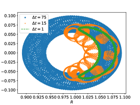
(a) BA2

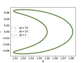
(b) RK4

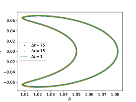
(c) VSI2

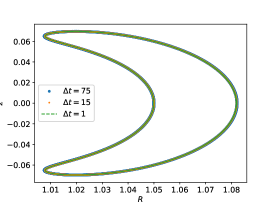
(d) BAP2

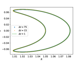
(e) VSIP2

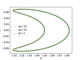
(f) GISIP2

Figure 1: Banana orbits calculated by different algorithms with different time-steps. All three structure-preserving geometric algorithms for the CPP dynamics (BAP2, GISIP2 and VSIP2) can accurately calculate the banana orbit as a slow manifold of the CPP with large time-steps.

For this set of parameters, the particle is trapped, and its projection on the $R-z$ plane is a banana orbit. When the time-step is larger than the gyro-period, the original Boris algorithm applied to the Newton’s equation of the classical particle (BA2) gives incorrect orbits. This indicates BA2 can not capture the slow drift motion in the tokamak geometry using large time-steps. All other five algorithms are stable at this time-scale and calculate the slow drift orbits correctly.

To demonstrate the long-term conservation property of structure-preserving geometric algorithms for the slow manifold dynamics of the CPP, we test the algorithms using a large time-step, i.e., $\Delta t=105$, and run the simulations for $1\times 10^{8}$ time-steps. The first and last turns of the banana orbit in the poloidal plane calculated by different algorithms are shown in Fig. 2. It is clear that all three structure-preserving geometric algorithms for the CPP dynamics (BAP2, GISIP2 and VSIP2) can calculate the banana orbit accurately as a slow manifold for $1\times 10^{8}$ time-steps, while the non-geometric RK4 algorithm can not. For the RK4 algorithm, the truncation error from each time-step accumulates coherently, and the energy of the discrete system monotonically decreases as a function of time. As a result of this numerical dissipation, the banana orbit shrinks towards the center of the device. This numerical error may mimic real physical effects such as the neoclassical Ware pinch (Ware, 1970). Without long-term accuracy, the long-term simulation results of the RK4 method are not reliable.

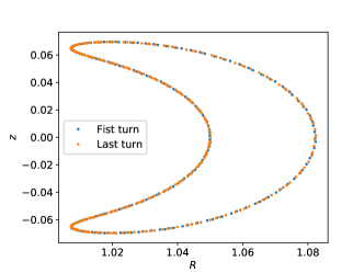
(a) BAP

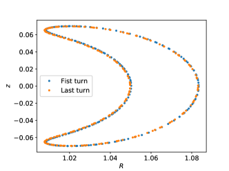
(b) GISIP2

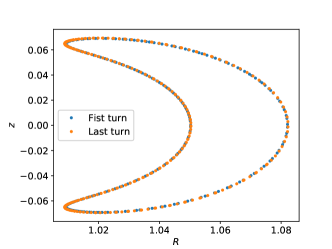
(c) VSIP2

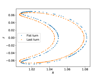
(d) RK4

Figure 2: Comparison of long-term accuracy of the three structure-preserving geometric algorithms (BAP2, GISIP2 and VSIP2) for the slow manifold dynamics of the CPP and the RK4 method. The time-step is $\Delta t=105$. The BAP2, GISIP2, and VSIP2 algorithms calculate the banana orbit accurately for $1\times 10^{8}$ time-steps. The energy error of the RK4 method accumulates coherently over time, and the long-terms simulation result is not trustworthy.

As discussed above, the variational symplectic integrators when applied to the guiding center Lagrangian $L_{\mathrm{gc}}$ lead to multi-step methods due to the degeneracy of the Lagrangian, and numerical solutions may be jeopardized by the unstable parasitic modes (Hairer et al., 2002; Hairer, 1999; Shang, 2011; Ellison et al., 2015; Ellison, 2016; Ellison et al., 2018). For the banana orbits in tokamaks, the unstable parasitic modes will become significant when the time-step is relatively small. To demonstrate this phenomenon, we perform long-term simulations with $\Delta t=6$ and $\Delta t=15$. The total number of time-steps is $1.67\times 10^{6}$ and $6.67\times 10^{5}$, respectively. The simulated orbits in $R-z$ plane are shown in Fig. 3. It can be found that orbits calculated by the implicit midpoint variational symplectic integrator applied to the guiding center Lagrangian $L_{\mathrm{gc}}$ (VSI2) are unstable, while the three structure-preserving geometric algorithms for the slow manifold dynamics of the CPP enjoy long-term stability and accuracy.

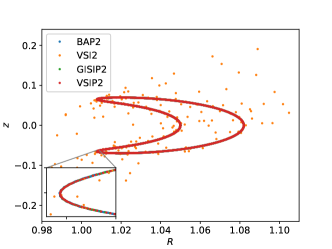
(a) $\Delta t=6$

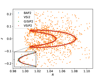
(b) $\Delta t=15$

Figure 3: Comparison of long-term stability and accuracy of the three structure-preserving geometric algorithms (BAP2, GISIP2 and VSIP2) for the slow manifold dynamics of the CPP and implicit midpoint variational symplectic integrator (VSI2) applied to the guiding center Lagrangian $L_{\mathrm{gc}}$. The time-steps are $\Delta t=6$ (a) and $\Delta t=15$ (b), and the total number of time-steps are $1.67\times 10^{6}$ (a) and $6.67\times 10^{5}$ (b). The VSI2 algorithm is unstable, while the BAP2, GISIP2, and VSIP2 algorithms are stable and accurate for long-term dynamics.

To summarize, we discovered that the slow manifolds of the classical Pauli particle enable a family of structure-preserving geometric algorithms for the guiding center dynamics. The mathematical difficulty associated with the unstable parasitic modes of the discrete guiding center Lagrangian has been overcome by the physics of the classical Pauli particle. Unlike the degenerate guiding center Lagrangian, the classical Pauli particle Lagrangian is regular, and variational and canonical symplectic integrators can be directly applied without introducing unstable parasitic modes. Three structure-preserving geometric algorithms have been implemented for the slow manifold dynamics of the classical Pauli particle. Numerical results confirmed that all three methods are stable with long-term accuracy in terms of calculating slow guiding center drift motions with time-steps significantly larger than the gyro-period. We expect that this technique of slow manifold to be effective for other degenerate Lagrangians reduced from regular Lagrangians.